Capturing pattern bi-stability dynamics in delay-coupled swarms

Abstract

Swarms of large numbers of agents appear in many biological and engineering fields. Dynamic bi-stability of co-existing spatio-temporal patterns has been observed in many models of large population swarms. However, many reduced models for analysis, such as mean-field (MF), do not capture the bifurcation structure of bi-stable behavior. Here, we develop a new model for the dynamics of a large population swarm with delayed coupling. The additional physics predicts how individual particle dynamics affects the motion of the entire swarm. Specifically, (1) we correct the center of mass propulsion physics accounting for the particles’ velocity distribution; (2) we show that the model we develop is able to capture the pattern bi-stability displayed by the full swarm model.

Nonlinear dynamics Pattern formation in complex systems Population dynamics

1 Introduction

Recently, much attention has been given to the study of interacting multi-agent, particle or swarming systems in various natural [1, 2, 3, 4] and engineering [5, 6] fields. These multi-agent swarms can self-organize and form complex spatio-temporal patterns even when the coupling between agents is weak. Many of these investigations have been motivated by a multitude of biological systems such as schooling fish, swarming locusts, flocking birds, bacterial colonies, ant movement, etc. [7, 8, 9, 10, 11, 12, 13, 14], and have also been applied to the design of systems of autonomous, communicating robots or agents [15, 16, 17] and mobile sensor networks [18, 19]. The excellent overviews [20, 21] discuss the diverse biological contexts where swarming occurs, as well as different modeling approaches. We note that in spite of all these investigations, understanding how swarming patterns self-organize, as well as predicting their stability are still very much open problems.

A number of different mathematical modeling techniques have been applied to investigate aggregating particle systems. One possibility is to treat the system at a single-individual level, using ordinary differential equations (ODEs) or delay differential equations (DDEs) to describe their motion in space and time [22, 23, 24, 25]. Another possibility that is applicable with sufficiently dense numbers of particles involves the use of continuum models with averaged velocity and agent density fields that are governed by partial differential equations (PDEs) [9, 26, 27, 11]. Moreoever, a number of researchers have incorporated random noise effects into their models that are able to produce transitions from one pattern to another [28, 29]. The study of these systems has been enriched by tools from statistical physics [30] since both first and second order phase transitions have been found in the formation of coherent states [22, 31].

An important aspect of understanding self-organizing swarms patterns is that of delay in the coupling between individual agents. Time delay appears in many systems for several reasons: 1) finite time information transfer; 2) time required to acquire measurement information; 3) computation time required for generating the control instructions; and 4) actuation time required for the instructions to be applied. In general, time delay reflects an important property inherited in all swarms due to actuation, control, communication, and computation [5, 32]. The occurrence of time delays in interacting particle systems and in dynamical systems in general has been shown to have profound dynamical consequences, such as destabilization and synchronization [33, 34]. Since time delays in the engineering of autonomous robot-systems are almost unavoidable, incorporating them into the mathematical models is particularly important. Initially, such studies focused on the case of one or a few discrete time delays. More recently, however, the complex situation of several and random time delays has been researched [35, 36, 37]. Another important case is that of distributed time delays, when the dynamics of the system depends on a continuous interval in its past instead of on a discrete instant [38, 39, 40].

When examining self-organizing patterns in swarms, different attractors emerge depending on initial conditions, and/or the the addition of external noise. Co-existing bi- and multi-stable swarming patterns have been observed in a multitude of models [41, 42, 43]. Because of the existence of co-existing patterns, time delayed swarming systems display transitions between different spatio-temporal patterns if there is an adequate balance between the strength of the attractive coupling, the duration of time delay and the external noise intensity, [29, 44, 45]. Often, mean-field approximations to swarm dynamics cannot capture the possibility of different patterns for the same parameter values [44]; this failure is a consequence of the mean field missing the details of the particle distribution about the swarm center of mass. To redress the bi-stable formation problem, we develop a new reduced model based on a higher-order approximation that is able to predict bi-stable patterns in globally coupled swarm models with delayed interactions.

2 The Reduced Swarm Model Derivation

We consider the dynamics of a two dimensional system of $N$ particles being acted on by the influence of self-propulsion and mutual attraction. Let $\mathbf{f}(\mathbf{r,\dot{r}})$, denote a self propelling force, and an interaction potential function between particles be given by $U(\mathbf{r}_{i}-\mathbf{r}_{j})$. In our description, the attraction between particles does not occur instantaneously, but rather in a time delayed fashion due to finite communication speeds and processing times. We describe the general motion of the particles by the following dimensionless equations:

$$\ddot{\mathbf{r}}_{i}(t)\mathbf{=\mathbf{f}}(\mathbf{\mathbf{r},\dot{r}}_{i})-\frac{a}{N}\sum_{j=1,j\neq i}^{N}\nabla_{\mathbf{r}_{i}}U(\mathbf{r}_{i}(t)-\mathbf{r}_{j}(t-\tau))$$ (1)

for $i=1,2\ldots,N$. Here, $\mathbf{r}_{i}(t)$ and $\dot{\mathbf{r}}_{i}(t)$ denote the two-dimensional position and velocity of particle $i$ at time $t$, respectively. We assume $\mathbf{f}(\mathbf{r},\dot{\mathbf{r}})=(1-\dot{\mathbf{r}}_{i}^{2})\dot{\mathbf{r}}_{i}$ to describe the self-propulsion of agent $i$, where $\dot{\mathbf{r}}_{i}^{2}=\dot{\mathbf{r}}_{i}\cdot\dot{\mathbf{r}}_{i}$. We denote the parameter $a$ as the coupling constant and measures the strength of attraction between agents. At time $t$, agent $i$ is attracted to the position of agent $j$ at the past time $t-\tau$. If we assume the form of our model is based on the normal form for particles near a supercritical bifurcation corresponding to the onset of coherent motion [46], then the leading term of the potential function may be considered to be quadratic; i.e., $\nabla_{\mathbf{r}_{i}}U(\mathbf{r}_{i}(t)-\mathbf{r}_{j}(t-\tau))=\mathbf{r}_{i}(t)-\mathbf{r}_{j}(t-\tau)$. Specific mathematical models of this kind have been extensively used to study the dynamics of swarm patterns [47, 28, 48, 29, 46, 44]. Certainly, the choice of potential function has a fundamental impact on the type of long-term patterns that the system may acquire as well as on determining their dimensionality and characteristic spatio-temporal length scales [49]; many of these scales may be explicitly obtained for the patterns arising from Eqs. (1) [44]. Numerous potential functions appropriate to different biological and engineering situations have been carefully investigated [3, 2]; most of them possess one or more minima where attraction and repulsion are balanced. Our potential may be thought of as a first, quadratic approximation to the minima of more complicated potential landscapes.

We obtain a reduced description for the swarm dynamics in Eqn. (1) by defining the center of mass of the swarm (CM), $\mathbf{R}(t)=\frac{1}{N}\sum_{i=1}^{N}\mathbf{r}_{i}(t)$, and the three tensors

$$\mathbf{C_{rr}}=\frac{1}{N}\sum_{i=1}^{N}\delta\mathbf{r}_{i}\delta\mathbf{r}_{i},\qquad\mathbf{C_{vv}}=\frac{1}{N}\sum_{i=1}^{N}\delta\dot{\mathbf{r}}_{i}\delta\dot{\mathbf{r}}_{i},$$ (2)

$$\mathbf{C_{rv}}=\frac{1}{N}\sum_{i=1}^{N}\delta\mathbf{r}_{i}\delta\dot{\mathbf{r}}_{i},$$

where $\delta\mathbf{r}_{i}=\mathbf{r}_{i}-\mathbf{R}$. The above tensors represent all of the second moments of the particles’ position and velocity relative to the center of mass. Here, $\mathbf{a}\mathbf{b}$ is the exterior product of the vectors $\mathbf{a}$ and $\mathbf{b}$ and has matrix components $(\mathbf{a}\mathbf{b})_{ij}=a_{i}b_{j}$. Note that $\mathbf{C_{rr}}$ and $\mathbf{C_{vv}}$ are  symmetric tensors with non-negative diagonal elements, whereas $\mathbf{C_{rv}}$ has neither of these properties.

The dynamical equation for the center of mass is obtained from the relation $\ddot{\mathbf{R}}(t)=\frac{1}{N}\sum_{i=1}^{N}\ddot{\mathbf{r}}_{i}(t)$, while the equations for the tensors are found by taking time derivatives of $\delta\mathbf{r}_{i}$ and recalling $\sum_{i}\delta\mathbf{r}_{i}=0$. In our derivation, we drop all possible third order moments (that take the form of third order tensors) and justify it as follows. The swarm equations are rotationally-invariant in space and so the time-asymptotic patterns that arise tend to have particle position and velocity distributions that are symmetric with respect to the CM. For large numbers of particles organized in such symmetric patterns, these third order moments are composed of mutually cancelling terms since they are of odd power in either in the position or the velocity relative to the CM. Finally, we close the system of equations by approximating fourth order moments of the form $\frac{1}{N}\sum_{i=1}^{N}\delta\dot{\mathbf{r}}^{2}_{i}\mathbf{a}_{i}\mathbf{b}_{i}$ (where $\mathbf{a}_{i}$ and $\mathbf{b}_{i}$ are either $\delta{\mathbf{r}}_{i}$ or $\delta\dot{\mathbf{r}}_{i}$) by

$$\frac{1}{N}\sum_{i=1}^{N}\left\langle\delta\dot{\mathbf{r}}^{2}_{i}\right\rangle\mathbf{a}_{i}\mathbf{b}_{i}=\textrm{tr}(\mathbf{C_{vv}})\ \frac{1}{N}\sum_{i=1}^{N}\mathbf{a}_{i}\mathbf{b}_{i},$$ (3)

and dropping all higher order moments. Here, $\textrm{tr}(\mathbf{C_{vv}})$ denotes the trace of $\mathbf{C_{vv}}$.

Our mean-field approximation including up to second moments (MF2M) finally takes the form:

$$\ddot{\mathbf{R}}= P(t)\dot{\mathbf{R}}-2\dot{\mathbf{R}}\cdot\mathbf{C_{vv}}-a\left(\mathbf{R}(t)-\mathbf{R}(t-\tau)\right),$$ (4a)

$$\ddot{\mathbf{C}}_{\mathbf{rr}}= 2\mathbf{C}_{\mathbf{vv}}-2\left(\dot{\mathbf{R}}\cdot{\mathbf{C}}_{\mathbf{vr}}\dot{\mathbf{R}}+\dot{\mathbf{R}}{\mathbf{C}}_{\mathbf{rv}}\cdot\dot{\mathbf{R}}\right)$$

$$\qquad+P(t)\dot{\mathbf{C}}_{\mathbf{rr}}-2a{\mathbf{C}}_{\mathbf{rr}},$$ (4b)

$$\dot{\mathbf{C}}_{\mathbf{rv}}= \mathbf{C}_{\mathbf{vv}}-2\dot{\mathbf{R}}\cdot{\mathbf{C}}_{\mathbf{vr}}\dot{\mathbf{R}}+P(t){\mathbf{C}}_{\mathbf{rv}}-a{\mathbf{C}}_{\mathbf{rr}},$$ (4c)

$$\dot{\mathbf{C}}_{\mathbf{vv}}= -2\left(\dot{\mathbf{R}}\cdot\mathbf{C_{vv}}\dot{\mathbf{R}}+\dot{\mathbf{R}}\mathbf{C_{vv}}\cdot\dot{\mathbf{R}}\right)+2P(t)\mathbf{C_{vv}}$$

$$\qquad-a\dot{\mathbf{C}}_{\mathbf{rr}},$$ (4d)

where we let $P(t)=\left(1-\dot{\mathbf{R}}^{2}-\textrm{tr}(\mathbf{C_{vv}})\right)$. Note that no evolution equation is needed for the tensor $\mathbf{C}_{\mathbf{vr}}$ since $\mathbf{C}_{\mathbf{vr}}=\mathbf{C}_{\mathbf{rv}}^{\top}$.

Interestingly, no second moment tensor appears in a time-delayed form. This is because the acceleration due to time delay that each particle and the center of mass undergo is the same, up to $\mathcal{O}(1/N)$. Thus, relative to the center of mass (as the second moment tensors are themselves measured) the particles undergo no time-delayed acceleration, to the order mentioned. Also, note that (i) Eqns. (4) reduce to the first-order mean-field approximation of [44] when all second-moment tensors are neglected; and that (ii) the linearization of Eqns. (4) about the trivial state decouples the CM and the second moment tensors. The standard linear stability calculation shows that second moment tensor equations render the trivial solution of Eqns. (4) unstable for all parameter values. The instability of the trivial solution agrees with what intuition tells us about Eqn. (1): the slightest difference in position or velocity among the particles will accelerate them via self-propulsive and attractive forces and make the CM and second-moment tensors depart from the stationary solution. This effect is not captured by the simple MF model since it does not account at all for how the particles are distributed about the center of mass.

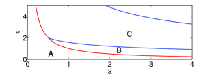
Figure 1: As in [44], Hopf (blue) and pitchfork (red) bifurcation curves in $a$ and $\tau$ space that delimit different regions of long-term dynamical behavior as prediceted by the first-order MF approximation: uniformly travelling state (A), ring state (B) and rotating state (C). (Color online)

3 Model analysis and physical interpretation

The velocity second moment introduces two corrections into the propulsion of the CM equation (4a) in a physically meaningful way. To see this, first note that while the self-propulsive force of each individual particle always lies along its velocity vector, the cumulative self-propulsion of all particles is not necessarily directed along the CM velocity vector. The first tensor correction accounts for how the particle dispersal slows down the CM propulsion along its velocity and appears in the term $P(t)\dot{\mathbf{R}}=\left(1-\dot{\mathbf{R}}^{2}-\textrm{tr}(\mathbf{C_{vv}})\right)\dot{\mathbf{R}}$. For example, consider that all particles move coherently with the exact same velocity vectors; since their self-propelling forces are also coherent the CM self-propulsion term $\left(1-\dot{\mathbf{R}}^{2}-\textrm{tr}(\mathbf{C_{vv}})\right)\dot{\mathbf{R}}$ is maximal, in the sense that $\textrm{tr}(\mathbf{C_{vv}})=0$. Otherwise, when the particles are becoming dispersed $\textrm{tr}(\mathbf{C_{vv}})>0$, their individual self-propulsion does not add up coherently and this makes the self-propulsion of the CM weaker. The second tensor correction is the term $-2\dot{\mathbf{R}}\cdot\mathbf{C_{vv}}$ and, since in contrast to the term $P(t)\dot{\mathbf{R}}$ it is not necessarily directed along the velocity vector $\dot{\mathbf{R}}$, it represents a correction for the fact that the CM propulsion may have a component orthogonal to $\dot{\mathbf{R}}$ because of the dispersal of particles.

An important consequence of (i) and (ii) is that all of the bifurcations found previously for the MF approximation [44] are inherited by the MF2M system in Eqns. (4). These bifurcation boundaries delimit the parameter regions where the MF approximation predicts different spatio-temporal patterns to be adopted in the long-time limit (Fig. 1). (A) A uniformly travelling state is composed of particles collapsed together and moving at constant speed in a given direction. (B) A ring state is formed by particles distributed almost uniformly along a circle, some of them moving clockwise and others counterclockwise, while the center of mass is at rest at the center (see Fig. 4a below). (C) A rotating state, in which all particles collapse to a point and move in a circular orbit (see Fig. 4b).

The spatio-temporal patterns (A), (B) and (C) are captured by our MF2M approximation and manifest themselves as follows. The uniformly travelling/rotating states have trivial components for the second moment tensors (indicating the collapse of all particles to the CM) but uniform motion/periodic oscillations for the position of the CM. In contrast, the ring state has a stationary position for the CM but periodic oscillations for all second moment tensor components. The periodic oscillations of the tensor components in the ring state are due to the fact that particles are not distributed quite uniformly along the ring in either position or velocity space and their spread about the CM (second moment tensors) in both spaces has periodic variations.

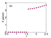
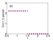
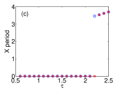
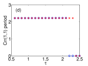
Figure 2: Period of sustained oscillations for the first component of the CM vector (left column) and the tensor component $C_{\mathbf{vv}}(1,1)$ (right column) for different values of the time delay $\tau$ and for $a=2$. Blue circles correspond to the full swarm described by Eqn. (1) and red crosses to our MF2M approximation. Initial conditions favor convergence to the rotating/ring state along the top/bottom row. The swarm converges to the ring state for $\tau\lesssim 1.5$ ($\tau\lesssim 2.1$) along the top (bottom) row and to the rotating state for higher $\tau$’s. In the ring state, the period of oscillation of $C_{\mathbf{vv}}(1,1)$ is approximately $\pi/\sqrt{a}=2.22$, as shown analytically. The agreement with other tensor components is similar. See text for more details. (Color online)

We employ numerical simulations using a fourth order Runge-Kutta algorithm with quadratic interpolation for the delayed terms to see how our MS2M system captures the convergence to different spatio-temporal patterns. The coupling parameter is fixed at $a=2$ and the time delay is varied so as to cross the boundary between regions B and C of Fig. 1. We consider two types of initial conditions over the interval $[-\tau,0]$: in the first, the particles are distributed at random in a box with sides of length 0.05 and velocities uniformly distributed in [0.5 0.55] for the $x$ component and in [-0.025 0.025] for the $y$ component. In the second initial condition we distribute $N=300$ particles at random in the unit box with velocity components randomly distributed between -0.5 and 0.5. The first initial condition favors convergence to the rotating state while the second one favors convergence to the ring state. We note that although the initial conditions for the position and velocity vectors appear physically inconsistent, this is of no consequence since no time-delayed velocity terms appear in the equations.

Starting from $\tau=0.5$, the full swarm and our MF2M systems first converge asymptotically to the ring state (Fig. 2). As the time delay increases, the convergence is to the rotating state instead. However, we find the hysterisis loop characteristic of bi-stable behavior: the transition occurs at different values of $\tau$ for the two different initial conditions. Remarkably, our MF2M system is not only able to accurately predict the periods of oscillation for the ring/rotating states of the full swarm equations, but it also identifies the value of the time delay at which the pattern transition occurs for each of the two initial conditions.

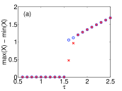
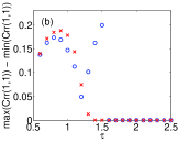
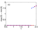
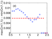
Figure 3: Oscillation amplitude of the first component of the CM vector (left column) and the tensor component $C_{\mathbf{vv}}(1,1)$ (right column), after the decay of transients, for different values of the time delay $\tau$ and for $a=2$. Blue circles correspond to the full swarm described by Eqn. (1) and red crosses to our MF2M approximation. Initial conditions favor convergence to the rotating/ring state along the top/bottom row. The swarm converges to the ring state for $\tau\lesssim 1.5$ ($\tau\lesssim 2.1$) along the top (bottom) row and to the rotating state for higher $\tau$’s. The agreement with other tensor components is similar. (Color online)

As noted above, the second moment tensors undergo periodic oscillations when the particles adopt the ring state. The period of these tensor oscillations may be approximated directly from Eqns. (4). In this spatio-temporal pattern, the CM is fixed and individual particles move at unit speed [44]. Substituting $\mathbf{R}=\dot{\mathbf{R}}=0$ and $\textrm{tr}(\mathbf{C_{vv}})=1$ in Eqns. (4) yields a linear system with oscillatory solutions with period $\pi/\sqrt{a}$. On the other hand, the period of oscillation of the center of mass position in the rotating state is determined by a complicated non-linear equation that may be obtained by resorting to polar coordinates and agrees perfectly with numerical simulations [44]. Thus, while the simple MF approximation fails to capture the bi-stable behavior displayed by the full swarm model, our MF2M approximation is able to do so.

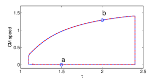
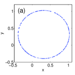
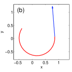
Figure 4: Top panel: hysterisis loop of the CM speed for the full model (solid blue) and our MF2M (dashed red) approximation, obtained with a time varying time delay (loop is traversed counter-clockwise in time). A zero/non-zero CM speed indicates convergence to the ring/rotating state. Transient dynamics at the time delay values where pattern switching occurs ($\tau=1.1$, 2.4) have been removed. Bottom panels: time snapshots of the spatial distribution of the swarm particles at the points labeled (a) and (b) of the top panel. In the rotating state of panel (b) all particles have collapsed to a point and move with the same velocity (blue arrow) around a circle; a portion of their time track is also shown (red line). (Color online).

An important signature of the spatio-temporal patterns of our system is the amplitude of oscillations, which we also extract from the results of our numerical simulations (Fig. 3). The hysterisis of the system becomes equally evident in these amplitude vs. time delay plots. For the two initial conditions described before, our MF2M model is able to capture the oscillation amplitude of the CM (Fig. 3, left column) with accuracy as well as the time delay value at which the long-time convergence switches from the ring to the rotating state. However, the amplitude of oscillation of the tensor component $C_{\mathbf{vv}xx}$ is not captured as well, particularly for time delay values near the MF bifurcation (Fig. 3, right column). This departure is due to the neglected higher-order moments and finite-particle effects.

An additional way to visualize the bistable nature of the ring and rotating state attractors is by forcing the system to undergo hysterisis via a time-dependent time delay. To this end, we start both the full swarm system and our MF2M approximation with a time delay of $\tau=1.1$, increase it slowly up to $\tau=2.4$ and then bring it back down to its starting value. Using the speed of the CM as a proxy for the state of the system, we see the swarm converge to the ring state (CM speed of zero) up until the time delay reaches 2.4; at this point, the swarm switches to the rotating state (non-zero CM speed) and persists in this state until the time delay is back to 1.1 (Fig. 4, top panel). Figs. 4(a) and (b) show snapshots of the swarm in different states, taken at the points indicated in the top panel.

4 Discussion and conlusions

A more realistic version of the model studied here should modify our choice of potential function to include the local, hard-body repulsion among individuals. Our previous work shows that the patterns and transitions discussed here do not fundamentally change with the addition of small, local repulsive forces between particles. Stronger repulsion certainly can destabilize the coherent structures. Crucially, we note that since repulsion causes the particles to spread out in space, their distribution about the center of mass becomes even more important for determining their group dynamics. Although a systematic study is beyond the scope of this work, we expect our extended MF2M model to be highly useful in frameworks where repulsion between particles cannot be neglected.

We also expect our multi-moment approach to extend the MF2M model framework to situations in which the time delay for inter-particle interactions is distributed. This situation is of interest since, analogously to inter-particle repulsion, randomly distributed time delays cause the individual agents to occupy larger portions of space, making their second moments non-negligible [45]. Conversely, in some realistic applications the particle distribution about the center of mass can have an effect on the magnitude of the time delay. In our MF2M framework, this would make the time delay be dependent on the second moment tensors.

To summarize, we derived a new MF approximation of a general model swarming system in order to account for higher order moments about the CM. Notably, our extended MF2M model is able to account for the bi-stability of spatio-temporal patterns that are displayed by the original swarming particles. This is in sharp contrast to the MF approximation for this system, which cannot capture this bi-stability and other complex behavior of the time delayed swarming system that we studied. With the inclusion of higher order moments, it is clear to what extent bi-stability depends on the particle distribution of the swarm about its center of mass. Adding the additional physics to the model, although higher dimensional than just a mean field, should allow more general low dimensional approaches to more accurately predict the structure of bi-stability in large population swarms.

- [1] \NameLukeman R., Li Y.-X. Edelstein-Keshet L. \REVIEWBulletin of Mathematical Biology712009352.
- [2] \NameMogilner A. Edelstein-Keshet L. \REVIEWJournal of Mathematical Biology381999534.
- [3] \NameMogilner A., Edelstein-Keshet L., Bent L. Spiros A. \REVIEWJournal of Mathematical Biology472003353.
- [4] \NameTopaz C. M., D’Orsogna M. R., Edelstein-Keshet L. Bernoff A. J. \REVIEWPlos Computational Biology82012e1002642.
- [5] \NameCao Y., Yu W., Ren W. Chen G. \REVIEWIndustrial Informatics, IEEE Transactions on92013427.
- [6] \NameLeonard N., Paley D., Lekien F., Sepulchre R., Fratantoni D. Davis R. \REVIEWProceedings of the IEEE95200748.
- [7] \NameParrish J. Hamner W. \BookAnimal groups in three dimensions: how species aggregate (Cambridge University Press, Cambridge, England) 1997.
- [8] \NameBudrene E. Berg H. \REVIEWNature376199549.
- [9] \NameToner J. Tu Y. \REVIEWPhys. Rev. Lett.7519954326.
- [10] \NameParrish J. K. \REVIEWScience284199999.
- [11] \NameTopaz C. Bertozzi A. \REVIEWSIAM Journal on Applied Mathematics652004152.
- [12] \NameFarrell F. D. C., Marchetti M. C., Marenduzzo D. Tailleur J. \REVIEWPhys. Rev. Lett.1082012248101.
- [13] \NameMishra S., Tunstrøm K., Couzin I. D. Huepe C. \REVIEWPhys. Rev. E862012011901.
- [14] \NameXue C., Budrene E. O. Othmer H. G. \REVIEWPLoS Comput Biol72011e1002332.
- [15] \NameLeonard N. Fiorelli E. \BookVirtual leaders, artificial potentials and coordinated control of groups in proc. of \BookProc. of the 40th IEEE Conference on Decision and Control. Vol. 3 2002 pp. 2968–2973.
- [16] \NameMorgan D. Schwartz I. B. \REVIEWPhys. Lett. A3402005121.
- [17] \NameChuang Y.-L., Huang Y. R., D’Orsogna M. R. Bertozzi A. L. \BookMulti-vehicle flocking: Scalability of cooperative control algorithms using pairwise potentials in proc. of \Bookthe 2007 IEEE Int. Conf. on Robotics and Automation. 2007 pp. 2292–2299.
- [18] \NameLynch K. M., Schwartz I. B., Yang P. Freeman R. A. \REVIEWIEEE Trans. Robotics242008710.
- [19] \NameRen W., Beard R. Atkins E. \REVIEWControl Systems, IEEE27200771.
- [20] \NameVicsek T. Zafeiris A. \REVIEWPhys. Rep.517201271.
- [21] \NameMarchetti M., Joanny J., Ramaswamy S., Liverpool T., Prost J., Rao M. Aditi Simha R. \REVIEWRev. Mod. Phys.8520131143.
- [22] \NameVicsek T., Czirók A., Ben-Jacob E., Cohen I. Shochet O. \REVIEWPhys. Rev. Lett.7519951226.
- [23] \NameFlierl G., Grünbaum D., Levins S. Olson D. \REVIEWJ. Theor. Biol.1961999397.
- [24] \NameCouzin I., Krause J., James R., Ruxton G. Franks N. \REVIEWJ. Theor. Biol.21820021.
- [25] \NameJusth E. Krishnaprasad P. \BookSteering laws and continuum models for planar formations in proc. of \BookProc. of the 42nd IEEE Conference on Decision and Control. Vol. 4 2004 pp. 3609–3614.
- [26] \NameToner J. Tu Y. \REVIEWPhys. Rev. E5819984828.
- [27] \NameEdelstein-Keshet L., Watmough J. Grunbaum D. \REVIEWJ. Math. Biol.361998515.
- [28] \NameErdmann U. Ebeling W. \REVIEWPhys. Rev. E712005051904.
- [29] \NameForgoston E. Schwartz I. B. \REVIEWPhy. Rev. E772008035203(R).
- [30] \NameCzirok A. Vicsek T. \REVIEWJ. Phys. A: Math. Gen.3019971375.
- [31] \NameAldana M., Dossetti V., Huepe C., Kenkre V. Larralde H. \REVIEWPhys. Rev. Lett.982007.
- [32] \NameBiggs J. D., Bennet D. J. Dadzie S. K. \REVIEWPhys. Rev. E852012016105.
- [33] \NameEnglert A., Heiligenthal S., Kinzel W. Kanter I. \REVIEWPhys. Rev. E832011046222.
- [34] \NameZuo Z., Yang C. Wang Y. \REVIEWPhys. Lett. A37420101989.
- [35] \NameAhlborn A. Parlitz U. \REVIEWPhys. Rev. E752007065202.
- [36] \NameWu D., Zhu S. Luo X. \REVIEWEurophys. Lett.86200950002.
- [37] \NameMarti A. C., Ponce C M. Masoller C. \REVIEWPhysica A3712006.
- [38] \NameOmi T. Shinomoto S. \REVIEWPhys. Rev. E772008046214.
- [39] \NameCai G. Q. Lin Y. K. \REVIEWPhys. Rev. E762007041913.
- [40] \NameDykman M. I. Schwartz I. B. \REVIEWPhys. Rev. E862012031145.
- [41] \NameAldana M., Larralde H. Vázquez B. \REVIEWInternational Journal of Modern Physics B2320093661.
- [42] \NameHuepe C., Zschaler G., Do A.-L. Gross T. \REVIEWNew Journal of Physics132011073022.
- [43] \NamePaley D., Leonard N., Sepulchre R. Couzin I. \REVIEW46th CDC conference proceedings20074851.
- [44] \NameMier-y-Teran-Romero L., Forgoston E. Schwartz I. B. \REVIEWIEEE TRO2820121034.
- [45] \NameMier-y-Teran-Romero L., Lindley B. Schwartz I. B. \REVIEWPhys. Rev. E862012056202.
- [46] \NameMikhailov A. S. Zanette D. \REVIEWPhys. Rev. E6019994571.
- [47] \NameD’Orsogna M., Chuang Y., Bertozzi A. Chayes L. \REVIEWPhys. Rev. Lett.962006104302.
- [48] \NameStrefler J., Erdmann U. Schimansky-Geier L. \REVIEWPhys. Rev. E782008031927.
- [49] \NameBalague, D.Carrillo J., Laurent T. Raoul G. \REVIEWArch. Rational Mech. Anal.20920131055.