Multi-Layer Potfit: An Accurate Potential Representation for Efficient High-Dimensional Quantum Dynamics

Abstract

The multi-layer multi-configuration time-dependent Hartree method (ML-MCTDH) is a highly efficient scheme for studying the dynamics of high-dimensional quantum systems. Its use is greatly facilitated if the Hamiltonian of the system possesses a particular structure through which the multi-dimensional matrix elements can be computed efficiently. In the field of quantum molecular dynamics, the effective interaction between the atoms is often described by potential energy surfaces (PES), and it is necessary to fit such PES into the desired structure. For high-dimensional systems, the current approaches for this fitting process either lead to fits that are too large to be practical, or their accuracy is difficult to predict and control.

This article introduces multi-layer Potfit (MLPF), a novel fitting scheme that results in a PES representation in the hierarchical tensor (HT) format. The scheme is based on the hierarchical singular value decomposition, which can yield a near-optimal fit and give strict bounds for the obtained accuracy. Here, a recursive scheme for using the HT-format PES within ML-MCTDH is derived, and theoretical estimates as well as a computational example show that the use of MLPF can reduce the numerical effort for ML-MCTDH by orders of magnitude, compared to the traditionally used Potfit representation of the PES. Moreover, it is shown that MLPF is especially beneficial for high-accuracy PES representations, and it turns out that MLPF leads to computational savings already for comparatively small systems with just four modes.

I Introduction

Still today, the accurate numerical treatment of quantum systems with many degrees of freedom (DOFs) is a challenging task. Just to represent the wavefunction, most approaches require an amount of data which scales exponentially with the number of dimensions, a situation which has become known as the curse of dimensionalitybel61. Worse, the quantum-mechanical expressions involve high-dimensional integrations (e.g. for computing matrix elements of operators), and sophisticated methods are necessary for treating this quadrature problem.

In recent years, progress on these problems has been made on multiple fronts. Sparse grid integration methods, as pioneered by Smolyaksmo63:240, have been used by Ávila and Carrington as well as by Lauvergnat and Nauts to compute vibrational spectra of 12D systemsavi11:054126; avi11:064101; lau13:xxx. Another approach, which is also taken in the present work, formally employs a full product grid but uses tensor decomposition techniques to represent wavefunctions and operators in a compact manner. Perhaps the most successful exponent of this approach is the multi-configuration time-dependent Hartree method (MCTDH)mey90:73; bec00:1; mey09:book; mey12:351 which employs a Tucker decompositiontuc63:122 for the wavefunction. If the Hamiltonian is suitably structured (more on that below), MCTDH can be used to treat realistic systems up to around 20Draa99:936; cat01:2088; mar05:204310; ven07:184303; ven09:034308; sch11:234307, and even more if the system is weakly correlated or if low accuracy is sufficientnes03:24; wan00:9948. The multi-layer generalization of the MCTDH scheme (ML-MCTDH), first formulated by Wang and Thosswan03:1289 and later reformulated by Mantheman08:164116 as a recursive algorithm for arbitrary layering schemes, has already been used to treat systems with hundreds of DOFswan03:1289; cra07:144503; wan10:78; wes11:184102; cra11:064504; ven11:044135; bor12:751. ML-MCTDH uses a tensor decomposition which has then become known in the mathematical literature as hierarchical tensor or hierarchical Tucker (HT) formathac09:706, and developing techniques for operating on tensors in HT- and related formats is an active field of research. The monograph by Hackbuschhac12 gives an in-depth overview of the state of the art, and may be supplemented by the recent literature survey in Ref. gra13:survey.

To overcome the quadrature problem, MCTDH requires that the Hamiltonian can be expressed as a sum of products of one- (or low-)dimensional operators. For the kinetic energy part of the Hamiltonian, this can readily be achieved by using a suitable coordinate system. Most notably, the polyspherical approach of Gatti et al.gat09:1 can yield an exact kinetic energy operator for arbitrary system sizes, and a software package (TANA) is available for carrying out this procedure automaticallyndo12:034107. For the potential energy part of the Hamiltonian, in general only model systems possess the desired sum-of-products form. But in quantum molecular dynamics, the accurate treatment of a realistic system requires the use of a potential energy surface (PES), which is usually obtained as a complicated analytical fit to a large set of electronic structure calculations. For spectroscopic applications, it may be sufficient to use normal modes and do a Taylor expansion of the PES, as in the vibronic coupling Hamiltonian modelkoe84:59 for which ML-MCTDH studies with up to 66Dmen12:134302; men13:014313 have been carried out. But a Taylor expansion is only locally a good fit to the PES, whereas for many applications (e.g. floppy molecules, or scattering) one needs a more globally good fit. The next paragraph will review several approaches for finding such a fit. But first it should be noted that the quadrature problem may alternatively be solved by employing time-dependent grids, as in Manthe’s CDVR methodman96:6989 which also works in conjunction with ML-MCTDHman09:054109, where it has been successfully used to treat a 189D system-bath problem which involved a 9D PESwes11:184102 as well as systems with global PES up to 21Dham11:224305; ham12:054105; wod12:11249; wes13:014309; wel12:244106. The drawback of this approach is that it requires an extreme amount of PES function evaluations, which can easily become a bottleneck for the calculation, and massively parallel architectures (like GPUs) may be needed to overcome this problemwel13:164118.

For high-dimensional systems, perhaps the currently most widely used method for fitting a PES into sum-of-products form is the $n$-mode representation ($n$-MR, also known as cut-HDMR) in which the PES is expressed as a sum of terms which each depend only on a subset of the coordinates. Expressing each such low-dimensional term as a sum of products is then a much easier task. MCTDH studies using this approach have been carried out for the Zundel cationven07:184302; ven09:234305 and for malonaldehydesch11:234307. However, great care and effort is required to obtain a suitable $n$-MR because the method is not variational, in the sense that adding more terms to the expansion is not guaranteed to lead to a more accurate potential representation. Another approach for obtaining a sum-of-products fit is the use of neural networks with exponential activation functionsman06:194105; pra13:6925, though it has not been demonstrated that this approach can scale to higher dimensions. From the perspective of tensor decompositions, the sum-of-products form corresponds to the so-called canonical or parallel factors or shortly CP tensor format. In this context, finding a sum-of-products fit means that, given a general higher-order tensor, one would wish to find an accurate CP approximation to it, but the number of summands (the CP-rank) should not be too high. It turns out that this is a difficult problem, due to the fact that the set of CP-tensors with fixed CP-rank is not closedsil08:1084. Nevertheless, some iterative procedures for solving this approximation problem exist (see Chapter 9.5 in Ref. hac12 for an overview), but their accuracy is hard to control as they may get stuck in local minima. The situation improves if one imposes additional structural constraints on the CP format, specifically, turning to the Tucker format (i.e. the format used by the MCTDH wavefunction) leads to the Potfit algorithmjae96:7974 which has later been re-derived and named higher-order singular value decompositionlat00:1253 (HOSVD). This method allows the efficient construction of near-optimal fits with controlled accuracy, and it is variational, i.e. the accuracy will increase if more terms are added. Due to this precise and predictable control of accuracy, Potfit is the method of choice for systems where it is affordable, and hence it has been used in numerous MCTDH studies to date.

Potfit suffers from two limitations. The first limitation is that the algorithm starts from a full-grid representation of the potential, and hence it is subject to the curse of dimensionality. Recently, Peláez and Meyer introduced the multigrid Potfit method (MGPF)pel13:014108 which addresses this limitation by employing two nested grids, a coarse one and a fine one. This can reduce the amount of data that needs to be processed by orders of magnitude, so that it may be feasible to treat systems with up to about 12D with MGPF. The second limitation of Potfit is that the number of terms in the Tucker representation still grows exponentially with dimensionality, which negatively affects the performance of (ML-)MCTDH, since their numerical effort depends linearly on this number of terms. Essentially, this problem has so far precluded the wider use of ML-MCTDH for large systems with general PES (except for the studies using CDVR).

The present article addresses this second limitation by employing the hierarchical Tucker format for representing the potential. In contrast to Potfit, this does not result in a sum-of-products structure for the potential energy operator, but in a hierarchical multi-layer structure, which motivates the name multi-layer Potfit (MLPF) for this new fitting procedure. It will be shown that this multi-layer operator structure, when used in conjunction with ML-MCTDH, leads to a solution of the quadrature problem which is vastly superior to the regular Potfit approach, in that it can reduce the numerical effort for ML-MCTDH by orders of magnitude. Additionally, MLPF preserves the variational nature of the fitting process, and very high-accuracy representations of the PES become feasible.

This article is organized as follows. Section II reviews the ML-MCTDH scheme. In Section III, multi-layer operators are introduced, and the scheme for using them within ML-MCTDH is derived. Section IV presents MLPF as a multi-layer generalization of Potfit. Section V discusses how the computational cost for ML-MCTDH is reduced by using MLPF, and points out some limitations of the new scheme. In Section VI, a computational example shows the actual benefits of MLPF. Section VII concludes. Two appendices describe the more technical details of MLPF and the computational cost analysis.

II Review of ML-MCTDH

The treatment of ML-MCTDH used in this article closely follows the approach of Mantheman08:164116 and its discussion in Ref. ven11:044135. However, the introduction of a new representation for the potential energy operator will require changes to the practical equations of motion for ML-MCTDH. Due to the increased complexity of these equations, it is beneficial to introduce a more compact notation for the quantities involved. In the recursive spirit of the resulting expressions, this new notation focuses on the relative position of a logical mode in the multi-layer tree, and keeping explicit track of the layer to which a mode belongs is not necessary. For completeness and consistency, this section presents Manthe’s ideas and equations in the new notation.

II.1 Wavefunction ansatz and notation

A quantum system with $d$ distinguishable degrees of freedom (DOFs) $q_{1},q_{2},\ldots,q_{d}$ is described by a wavefunction $\psi$ which depends on these coordinates (and on time $t$). To treat this system computationally, one can employ for each DOF $f$ a set of $N_{f}$ time-independent orthonormal basis functions $\chi^{[f]}_{\alpha}(q_{f})$ (henceforth called primitive basis functions), and expand $\psi$ in the resulting product basis:

$$\psi(q_{1},\ldots,q_{d},t)$$

$$\quad=\sum_{\alpha_{1}=1}^{N_{1}}\cdots\sum_{\alpha_{d}=1}^{N_{d}}B_{\alpha_{1}\cdots\alpha_{d}}(t)\chi^{[1]}_{\alpha_{1}}(q_{1})\cdots\chi^{[d]}_{\alpha_{d}}(q_{d})$$ (1)

The problem with this standard method is that the size of $B$ scales exponentially with $d$, namely $\#B=\prod_{f=1}^{d}N_{f}=N^{d}$ (where $N$ is the geometric mean of the $N_{f}$). One approach for solving this problem is the Multi-Configuration Time-Dependent Hartree (MCTDH) methodmey90:73; bec00:1; mey09:book; mey12:351 which expands $\psi$ in smaller sets of time-dependent orthonormal basis functions $\varphi^{[f]}_{i}(q_{f},t)$, $i=1\ldots n_{f}$. These single-particle functions (SPFs) are in turn expanded in the primitive bases:

$$\psi(q_{1},\ldots,q_{d},t) =\sum_{i_{1}=1}^{n_{1}}\cdots\sum_{i_{d}=1}^{n_{d}}A_{i_{1}\cdots i_{d}}(t)$$

$$\qquad\times\varphi^{[1]}_{i_{1}}(q_{1},t)\cdots\varphi^{[d]}_{i_{d}}(q_{d},t)$$ (2)

$$\varphi^{[f]}_{i}(q_{f},t) =\sum_{\alpha=1}^{N_{f}}A^{[f]}_{i;\alpha}(t)\chi^{[f]}_{\alpha}(q_{f})\>\>;\>f=1\ldots d$$ (3)

This representation of $\psi$ requires $\sim n^{d}+dnN$ storage (where $n$ is a mean value of the $n_{f}$) for $A$ and the $A^{[f]}$, which is much lower than the storage requirement for $B$ if $n\ll N$. By experience, $n$ can be smaller than $N$ by a factor between 2 and 10, depending on the system and the required accuracy of the representation.

Yet, MCTDH does not get rid of the curse of dimensionality, it just alleviates it by lowering the base of the exponential scaling. Further computational savings can be gained by grouping DOFs together into logical modes $Q_{\kappa}$, $\kappa=1\ldots p$, such that the $\kappa$-th mode contains the DOFs $a_{\kappa}$ through $b_{\kappa}$, and then employing multi-dimensional SPFs:

$$Q_{\kappa} =(q_{a_{\kappa}},\ldots,q_{b_{\kappa}})\>\>;\>\kappa=1\ldots p$$ (4)

$$\psi(Q_{1},\ldots,Q_{p},t) =\sum_{i_{1}=1}^{\tilde{n}_{1}}\cdots\sum_{i_{p}=1}^{\tilde{n}_{p}}A_{i_{1}\cdots i_{p}}(t)$$

$$\qquad\times\varphi^{(1)}_{i_{1}}(Q_{1},t)\cdots\varphi^{(p)}_{i_{p}}(Q_{p},t)$$ (5)

$$\varphi^{(\kappa)}_{i}(Q_{\kappa},t) =\sum_{\alpha_{1}=1}^{N_{a_{\kappa}}}\cdots\sum_{\alpha_{d_{\kappa}}=1}^{N_{b_{\kappa}}}A^{(\kappa)}_{i;\alpha_{1}\cdots\alpha_{d_{\kappa}}}(t)$$

$$\qquad\times\chi^{[a_{\kappa}]}_{\alpha_{1}}(q_{a_{\kappa}})\cdots\chi^{[b_{\kappa}]}_{\alpha_{d_{\kappa}}}(q_{b_{\kappa}})$$ (6)

$$\qquad(i=1\ldots\tilde{n}_{\kappa}\quad;\quad d_{\kappa}:=b_{\kappa}-a_{\kappa}+1)$$

This mode combination reduces the storage requirements to $\sim\tilde{n}^{p}+p\tilde{n}N^{d/p}$. As a rule of thumb, the number of multi-dimensional SPFs that is necessary to keep the same level of accuracy as when using one-dimensional SPFs, is $\tilde{n}_{\kappa}\approx n_{a_{\kappa}}+\cdots+n_{b_{\kappa}}$, or in short $\tilde{n}\approx nd/p$. With this rule, now also the exponent of the exponential scaling rule is reduced, which further alleviates the curse of dimensionality. However, in practice one can group only $d_{\kappa}=2\ldots 4$ DOFs into one mode, because otherwise the effort for treating the multi-dimensional SPFs ($\sim N^{d_{\kappa}}$) becomes prohibitive.

But the computational effort can be further reduced by introducing another layer of basis functions and expansion coefficients. In this scheme, one first groups the DOFs into a moderate number of modes (say, $p=2\ldots 4$), and then splits each mode $Q_{\kappa}$ into sub-modes $Q_{\kappa,1},\ldots,Q_{\kappa,p_{\kappa}}$. Then one introduces sub-SPFs $\varphi^{(\kappa,\lambda)}_{j}(Q_{\kappa,\lambda},t)$ ($j=1\ldots n_{\kappa,\lambda}$) and expands the SPFs $\varphi^{(\kappa)}_{i}(Q_{\kappa},t)$ in products of these sub-SPFs (now dropping the tilde from the SPF numbers):

$$\psi(Q_{1},\ldots,Q_{p},t) =\sum_{i_{1}=1}^{n_{1}}\cdots\sum_{i_{p}=1}^{n_{p}}A_{i_{1}\cdots i_{p}}(t)\,$$

$$\qquad\times\varphi^{(1)}_{i_{1}}(Q_{1},t)\cdots\varphi^{(p)}_{i_{p}}(Q_{p},t)$$ (7)

$$\varphi^{(\kappa)}_{i}(Q_{\kappa},t) =\sum_{j_{1}=1}^{n_{\kappa,1}}\cdots\sum_{j_{p_{\kappa}}=1}^{n_{\kappa,p_{\kappa}}}A^{(\kappa)}_{i;j_{1}\cdots j_{p_{\kappa}}}\!(t)\,$$

$$\qquad\times\varphi^{(\kappa,1)}_{j_{1}}(Q_{\kappa,1},t)\cdots\varphi^{(\kappa,p_{\kappa})}_{j_{p_{\kappa}}}(Q_{\kappa,p_{\kappa}},t)$$ (8)

The sub-SPFs themselves are either expanded in the primitive bases,

$$\varphi^{(\kappa,\lambda)}_{j}(Q_{\kappa,\lambda},t) =\sum_{\alpha_{1}=1}^{N_{a_{\kappa,\lambda}}}\cdots\sum_{\alpha_{d_{\kappa,\lambda}}=1}^{N_{b_{\kappa,\lambda}}}A^{(\kappa,\lambda)}_{j;\alpha_{1}\cdots\alpha_{d_{\kappa,\lambda}}}\!(t)\,$$

$$\qquad\times\chi^{[a_{\kappa,\lambda}]}_{\alpha_{1}}(q_{a_{\kappa,\lambda}})\cdots\chi^{[b_{\kappa,\lambda}]}_{\alpha_{d_{\kappa,\lambda}}}(q_{b_{\kappa,\lambda}})\>,$$ (9)

or, if the mode $Q_{\kappa,\lambda}$ is too big to do so, it is expanded in another set of sub-sub-SPFs which depend on sub-sub-modes $Q_{\kappa,\lambda,\mu}$, and so on. This multi-layer MCTDH (ML-MCTDH) representation of $\psi$ is very flexible and rather compact (in terms of the total number of expansion coefficients). Manthe estimatesman08:164116 that, under moderate assumptions, the storage requirements for an ML-MCTDH wavefunction scale polynomially in $d$ ($d^{3}$ seems a realistic value).

Figure 1: An example for the hierarchical organization of the physical degrees of freedom $q_{f}$ into logical modes $Q_{z}$. The edges are labeled with the numbers $N_{f}$ of primitive basis functions for DOF $f$ or the numbers $n_{z}$ of SPFs for node $z$, respectively.

The successive splitting of the modes into sub-modes, sub-sub-modes etc. leads to a hierarchy of modes, which is best visualized as a tree structure (the ML-tree), as exemplified by Fig. 1. Then each (sub…-)mode can be labeled by its corresponding node in this tree structure. A node $z$ is specified by the path through which it can be reached from the top node, i.e. $z=(\kappa,\lambda,\ldots)$. To specify that the node $z^{\prime}$ is the $\mu$-th child node of $z$, one appends $\mu$ to this path, in short $z^{\prime}=(z,\mu)$. For consistency of notation, the top node itself is specified by an empty path, $z=\varnothing$. Its corresponding mode $Q_{\varnothing}$ is the total mode containing all degrees of freedom, and its sub-modes are the original modes $Q_{1},\ldots,Q_{p}$. In general, a mode $Q_{z}$ either has $p_{z}$ sub-modes $Q_{z,1},\ldots,Q_{z,p_{z}}$, or it contains $d_{z}$ degrees of freedom $q_{a_{z}},\ldots,q_{b_{z}}$ ($d_{z}=b_{z}-a_{z}+1$). In the first case, $z$ is called an internal node, while in the latter case, $z$ is called a leaf node and $Q_{z}$ is called a primitive mode. Leaf nodes may also be labeled by its DOFs, i.e. $z={[a_{z},\ldots,b_{z}]}$.

To shorten the notation, observe that the SPFs $\varphi^{(z)}_{i}(Q_{z})$ are elements of a Hilbert space $\mathcal{H}^{(z)}$ (usually chosen as the space of square-integrable functions over $Q_{z}$). Hence by specifying the superscript, it is clear to which Hilbert space $\varphi^{(z)}_{i}$ belongs, and on which mode it depends. Then the total wavefunction can be concisely expressed as a tensor product, i.e. Eq. (7) becomes

$$\psi(t)=\sum_{i_{1}=1}^{n_{1}}\cdots\sum_{i_{p}=1}^{n_{p}}A_{i_{1}\cdots i_{p}}(t)\,\varphi^{(1)}_{i_{1}}(t)\otimes\cdots\otimes\varphi^{(p)}_{i_{p}}(t)\>,$$ (10)

and likewise Eq. (8) can be re-expressed as

$$\varphi^{(\kappa)}_{i}(t) =\sum_{j_{1}=1}^{n_{\kappa,1}}\cdots\sum_{j_{p_{\kappa}}=1}^{n_{\kappa,p_{\kappa}}}A^{(\kappa)}_{i;j_{1}\cdots j_{p_{\kappa}}}\!(t)$$

$$\qquad\times\varphi^{(\kappa,1)}_{j_{1}}(t)\otimes\cdots\otimes\varphi^{(\kappa,p_{\kappa})}_{j_{p_{\kappa}}}(t)\>.$$ (11)

More generally, for internal nodes, the SPFs are expressed as

$$\varphi^{(z)}_{i}(t) =\sum_{j_{1}=1}^{n_{z,1}}\cdots\sum_{j_{p_{z}}=1}^{n_{z,p_{z}}}A^{(z)}_{i;j_{1}\cdots j_{p_{z}}}\!(t)$$

$$\qquad\times\varphi^{(z,1)}_{j_{1}}(t)\otimes\cdots\otimes\varphi^{(z,p_{z})}_{j_{p_{z}}}(t)\>,$$ (12)

while for leaf nodes, they are expressed in terms of primitive basis functions,

$$\varphi^{(z)}_{i}(t)=\sum_{\alpha_{1}=1}^{N_{a_{z}}}\cdots\sum_{\alpha_{d_{z}}=1}^{N_{b_{z}}}A^{(z)}_{i;\alpha_{1}\cdots\alpha_{d_{z}}}\!(t)\,\chi^{[a_{z}]}_{\alpha_{1}}\otimes\cdots\otimes\chi^{[b_{z}]}_{\alpha_{d_{z}}}\>.$$ (13)

To further simplify notation, the time-dependence of the SPFs $\varphi^{(z)}_{i}$ and of the expansion coefficients $A^{(z)}_{i;\cdots}$ should by now be clear and will no longer be mentioned unless necessary. Additionally, by defining a multi-index $J^{z}$ for node $z$ as

$$J^{z}=\begin{cases}(j_{1},\ldots,j_{d_{z}})\>\>;\>j_{f}=1\ldots N_{a_{z}+f-1}&\text{if $z$ is a leaf}\\ (j_{1},\ldots,j_{p_{z}})\>\>;\>j_{\kappa}=1\ldots n_{z,\kappa}&\text{\hskip-10.00002ptif $z$ is internal}\end{cases}$$ (14)

and by introducing the configurations $\Phi^{(z)}_{J^{z}}$ as

$$\Phi^{(z)}_{J^{z}}=\begin{cases}\chi^{[a_{z}]}_{j_{1}}\otimes\cdots\otimes\chi^{[b_{z}]}_{j_{d_{z}}}&\text{if $z$ is a leaf}\\[4.30554pt] \varphi^{(z,1)}_{j_{1}}\otimes\cdots\otimes\varphi^{(z,p_{z})}_{j_{p_{z}}}&\text{if $z$ is internal}\end{cases}$$ (15)

all SPFs can consistently be expanded as

$$\varphi^{(z)}_{i}=\sum_{J^{z}}A^{(z)}_{i;J^{z}}\Phi^{(z)}_{J^{z}}\quad.$$ (16)

Eq. (16) can even include the total wavefunction $\psi$ if one uses $p_{\varnothing}=p$, $n_{\varnothing}=1$, and sets $\varphi^{\varnothing}_{1}=\psi$. That is, the total wavefunction can be seen as a single SPF depending on the total mode. For simplicity, one may omit the index $i=1$, as it is implied by the top node, and use $\varphi^{\varnothing}$ for the total wavefunction:

$$\varphi^{\varnothing}=\sum_{J^{\varnothing}}A^{\varnothing}_{J^{\varnothing}}\Phi^{\varnothing}_{J^{\varnothing}}$$ (17)

It is often useful to distinguish the part of the total wavefunction that depends on a certain mode $Q_{z}$ from the part which depends on all other coordinates, $Q_{\varnothing}\!\setminus\!Q_{z}$. The part that depends on $Q_{z}$ can be expressed by the SPFs of node $z$, while the complementary part defines the single-hole functions (SHFs) $\Psi^{(z)}_{l}$:

$$\varphi^{\varnothing}(Q_{\varnothing})=\sum_{l=1}^{n_{z}}\Psi^{(z)}_{l}(Q_{\varnothing}\!\setminus\!Q_{z})\,\varphi^{(z)}_{l}(Q_{z})$$ (18)

That is, the SHFs are given by projecting out one particular SPF from the total wavefunction, namely

$$\Psi^{(z)}_{l}=\langle\varphi^{(z)}_{l}|\varphi^{\varnothing}\rangle\quad.$$ (19)

For the top node, this leads to one trivial SHF, namely $\Psi^{\varnothing}=\langle\varphi^{\varnothing}|\varphi^{\varnothing}\rangle=1$, which does not depend on any coordinates. For other nodes, there is a useful recursion relation for expressing the SHFs. Any node $z^{\prime}$ other than the top node is a child of some node $z$, i.e. $z^{\prime}=(z,\kappa)$ if it is the $\kappa$-th child. The SHFs of such a node $z^{\prime}$ can be written as

$$\Psi^{(z,\kappa)}_{l} =\langle\varphi^{(z,\kappa)}_{l}|\varphi^{\varnothing}\rangle=\Bigl{\langle}\varphi^{(z,\kappa)}_{l}\Bigr{|}\Bigr{.}\sum_{m=1}^{n_{z}}\Psi^{(z)}_{m}\otimes\varphi^{(z)}_{m}\Bigr{\rangle}$$

$$=\Bigl{\langle}\varphi^{(z,\kappa)}_{l}\Bigl{|}\Bigr{.}\sum_{m=1}^{n_{z}}\Psi^{(z)}_{m}\otimes\sum_{J^{z}}A^{(z)}_{m;J^{z}}\bigotimes_{\lambda=1}^{p_{z}}\varphi^{(z,\lambda)}_{j_{\lambda}}\Bigr{\rangle}$$

$$=\sum_{m=1}^{n_{z}}\sum_{{J}^{{z}\!\setminus\!{\kappa}}}A^{(z)}_{m;{J}^{{z}\!\setminus\!{\kappa}}_{\phantom{{z}\!\setminus\!}{l}}}\Psi^{(z)}_{m}\otimes\bigotimes_{\lambda\neq\kappa}\varphi^{(z,\lambda)}_{j_{\lambda}}$$ (20)

where ${J}^{{z}\!\setminus\!{\kappa}}$ and ${J}^{{z}\!\setminus\!{\kappa}}_{\phantom{{z}\!\setminus\!}{l}}$ denote multi-indices with a skipped or replaced index,

$${J}^{{z}\!\setminus\!{\kappa}} =(j_{1},\ldots,j_{\kappa-1},\phantom{l,}\,j_{\kappa+1},\ldots,j_{p_{z}})$$ (21)

$${J}^{{z}\!\setminus\!{\kappa}}_{\phantom{{z}\!\setminus\!}{l}} =(j_{1},\ldots,j_{\kappa-1},l,j_{\kappa+1},\ldots,j_{p_{z}})\quad.$$ (22)

Eq. (20) means that the SHFs of a node $(z,\kappa)$ can be expressed in terms of the SHFs and $A$-coefficients of its parent node $z$ plus the SPFs of the sibling nodes $(z,\lambda)$, $\lambda\neq\kappa$. Specifically, the $A$-coefficients of node $(z,\kappa)$ and its children are not needed to express its SHFs.

II.2 Equations of motion

The time-evolution of the total wavefunction under the action of a Hamiltonian operator $\hat{H}$ can be obtained by inserting the recursive expansion Eqs. (16,15) into the Dirac-Frenkelfre34 variational principle,

$$\langle\delta\varphi^{\varnothing}|\hat{H}-i\frac{\partial}{\partial t}|\varphi^{\varnothing}\rangle=0\quad.$$ (23)

The quantities being varied are all the SPFs of all nodes throughout the ML-tree, which means that all coefficients $A^{(z)}_{l;J^{z}}$ are being varied. In order to maintain the orthonormality of the SPFs, one may impose the constraints

$$i\langle\varphi^{(z)}_{l}|\dot{\varphi}^{(z)}_{m}\rangle =\langle\varphi^{(z)}_{l}|\hat{g}^{(z)}|\varphi^{(z)}_{m}\rangle$$

$$\quad\forall z\neq\varnothing\quad\forall\,l,m=1\ldots n_{z}$$ (24)

where $\hat{g}^{(z)}$ is a Hermitian (but otherwise arbitrary) operator acting on $Q_{z}$. In practice, $\hat{g}^{(z)}=0$ is used, and the further discussion will be restricted to this case.

The variational procedure leads to equations of motion (EOMs) for the $A$-coefficients. For the top node, one obtains

$$i\dot{A}^{\varnothing}_{J^{\varnothing}}=\sum_{K^{\varnothing}}\,\langle\Phi^{\varnothing}_{J^{\varnothing}}|\hat{H}|\Phi^{\varnothing}_{K^{\varnothing}}\rangle\,A^{\varnothing}_{K^{\varnothing}}\quad,$$ (25)

and for all other nodes

$$i\dot{A}^{(z)}_{l;J^{z}} =\sum_{K^{z}}\,\Bigl{\langle}\Phi^{(z)}_{J^{z}}\Bigl{|}(1-\hat{P}^{(z)})$$

$$\qquad\times\sum_{i=1}^{n_{z}}(\rho^{(z)})^{-1}_{li}\sum_{m=1}^{n_{z}}\langle\hat{H}\rangle^{(z)}_{im}\Bigr{|}\Phi^{(z)}_{K^{z}}\Bigr{\rangle}\,A^{(z)}_{K^{z}}$$ (26)

where $\hat{P}^{(z)}$ is a projector onto the space spanned by the SPFs of node $z$,

$$\hat{P}^{(z)} =\sum_{l=1}^{n_{z}}|\varphi^{(z)}_{l}\rangle\langle\varphi^{(z)}_{l}|$$ (27)

$$=\sum_{l=1}^{n_{z}}\sum_{J^{z}}\sum_{K^{z}}A^{(z)}_{l;J^{z}}A^{(z)*}_{l;K^{z}}|\Phi^{(z)}_{J^{z}}\rangle\langle\Phi^{(z)}_{K^{z}}|\quad,$$ (28)

$(\rho^{(z)})^{-1}$ is the inverse of the density matrix $\rho^{(z)}$ whose elements are given by the overlaps of the SHFs of node $z$,

$$\rho^{(z)}_{lm}=\langle\Psi^{(z)}_{l}|\Psi^{(z)}_{m}\rangle\quad,$$ (29)

and $\langle\hat{H}\rangle^{(z)}$ is a matrix of mean-field operators defined by

$$\langle\hat{H}\rangle^{(z)}_{lm}=\langle\Psi^{(z)}_{l}|\hat{H}|\Psi^{(z)}_{m}\rangle\quad.$$ (30)

Note that each $\langle\hat{H}\rangle^{(z)}_{lm}$ is an operator on the coordinate $Q_{z}$, as Eq. (30) only integrates over the coordinates $Q_{\varnothing}\!\setminus\!Q_{z}$.

II.3 Hamiltonian in Sum-of-Products Form

In this and the following sections, the expressions involving leaf nodes will be restricted to the case where the primitive modes contain only a single DOF. While the more general case is very relevant in practice, this restriction simplifies the notation, and the generalization of the expressions given here to primitive modes with more than one DOF is straightforward.

In order for ML-MCTDH to be efficient, one needs a fast way to evaluate the right-hand side of the equations of motion (25,II.2). In these, the most expensive part is the computation of the terms

$$\bigl{\langle}\Phi^{(z)}_{J^{z}}\bigr{|}\langle\hat{H}\rangle^{(z)}_{lm}\bigl{|}\Phi^{(z)}_{K^{z}}\bigr{\rangle}=\bigl{\langle}\Phi^{(z)}_{J^{z}}\otimes\Psi^{(z)}_{l}\bigr{|}\hat{H}\bigl{|}\Phi^{(z)}_{K^{z}}\otimes\Psi^{(z)}_{m}\bigr{\rangle}\quad.$$ (31)

Each of these terms constitutes (formally) a $d$-dimensional integration. This quadrature problem can be solved rather efficiently if the Hamiltonian has the form of a sum of products of one-dimensional operators,

$$\hat{H}=\sum_{r=1}^{s}c_{r}\hat{H}_{r}\quad\text{with}\quad\hat{H}_{r}=\bigotimes_{f=1}^{d}\hat{h}^{[f]}_{r}\quad.$$ (32)

For each node $z$, each $\hat{H}_{r}$ can be factored into an operator $\hat{h}^{(z)}_{r}$ acting on $Q_{z}$ and an operator $\hat{\mathcal{H}}^{(z)}_{r}$ acting on $Q_{\varnothing}\!\setminus\!Q_{z}$:

$$\hat{H}_{r}=\hat{h}^{(z)}_{r}\otimes\hat{\mathcal{H}}^{(z)}_{r}=\bigotimes_{f\in Q_{z}}\hat{h}^{[f]}_{r}\;\otimes\;\bigotimes_{f\notin Q_{z}}\hat{h}^{[f]}_{r}$$ (33)

As Manthe has shownman08:164116, this structure of the Hamiltonian permits a recursive scheme for evaluating the terms from Eq. (31). They can be expressed as

$$\bigl{\langle}\Phi^{(z)}_{J^{z}}\bigr{|}\langle\hat{H}\rangle^{(z)}_{lm}\bigl{|}\Phi^{(z)}_{K^{z}}\bigr{\rangle}$$

$$=\begin{cases}\displaystyle\sum_{r=1}^{s}c_{r}\,\mathfrak{H}^{(z)}_{r,lm}\,\bigl{\langle}\chi^{[f]}_{J^{z}}\bigl{|}\hat{h}^{[f]}_{r}\bigr{|}\chi^{[f]}_{K^{z}}\bigr{\rangle}&\text{if $z$ is a leaf, $z={[f]}$}\\[10.00002pt] \displaystyle\sum_{r=1}^{s}c_{r}\,\mathfrak{H}^{(z)}_{r,lm}\prod_{\kappa=1}^{p_{z}}\mathfrak{h}^{(z,\kappa)}_{r,j_{\kappa}k_{\kappa}}&\text{otherwise}\end{cases}$$ (34)

where the $\mathfrak{H}$- and $\mathfrak{h}$-terms are defined by

$$\mathfrak{h}^{(z)}_{r,jk} =\langle\varphi^{(z)}_{j}|\hat{h}^{(z)}_{r}|\varphi^{(z)}_{k}\rangle$$ (35)

$$\mathfrak{H}^{(z)}_{r,lm} =\langle\Psi^{(z)}_{l}|\hat{\mathcal{H}}^{(z)}_{r}|\Psi^{(z)}_{m}\rangle$$ (36)

and which can be evaluated recursively:

$$\mathfrak{h}^{(z)}_{r,jk} =\begin{cases}\displaystyle\sum_{\alpha=1}^{N_{f}}\sum_{\beta=1}^{N_{f}}A^{(z)*}_{j;\alpha}A^{(z)}_{k;\beta}\,\bigl{\langle}\chi^{[f]}_{\alpha}\bigl{|}\hat{h}^{[f]}_{r}\bigr{|}\chi^{[f]}_{\beta}\bigr{\rangle}&\text{if $z={[f]}$}\\ \displaystyle\sum_{I^{z}}\sum_{L^{z}}A^{(z)*}_{j;I^{z}}A^{(z)}_{k;L^{z}}\prod_{\kappa=1}^{p_{z}}\mathfrak{h}^{(z,\kappa)}_{r,i_{\kappa}l_{\kappa}}&\text{otherwise}\end{cases}$$ (37)

$$\mathfrak{H}^{\varnothing}_{r,11} =1$$ (38)

$$\mathfrak{H}^{(z,\kappa)}_{r,lm} =\sum_{a=1}^{n_{z}}\sum_{b=1}^{n_{z}}\mathfrak{H}^{(z)}_{r,ab}\sum_{{J}^{{z}\!\setminus\!{\kappa}}}\sum_{{K}^{{z}\!\setminus\!{\kappa}}}A^{(z)*}_{a;{J}^{{z}\!\setminus\!{\kappa}}_{\phantom{{z}\!\setminus\!}{l}}}A^{(z)}_{b;{K}^{{z}\!\setminus\!{\kappa}}_{\phantom{{z}\!\setminus\!}{m}}}\prod_{\lambda\neq\kappa}\mathfrak{h}^{(z,\lambda)}_{r,j_{\lambda}k_{\lambda}}$$ (39)

Eq. (37) expresses the $\mathfrak{h}$-terms for node $z$ in terms of the $\mathfrak{h}$-terms of its child nodes $(z,\kappa)$, which suggests a recursive “bottom-up” evaluation order, starting at the bottom layer where the $\mathfrak{h}$-terms depend on the matrix elements of the one-dimensional operators $\hat{h}^{[f]}_{r}$ in the primitive bases. On the other hand, Eq. (39) expresses the $\mathfrak{H}$-terms for a node $(z,\kappa)$ in terms of the $\mathfrak{H}$-terms of its parent node $z$ and the $\mathfrak{h}$-terms of its sibling nodes $(z,\lambda),\lambda\neq\kappa$, leading to a “top-down” recursive evaluation, starting from the top node where $\mathfrak{H}^{\varnothing}_{r}=1$.

For a Hamiltonian in form (32), using Eq. (34) yields the following explicit EOMs for the $A$-coefficients: For the top node

$$i\dot{A}^{\varnothing}_{J^{\varnothing}}= \sum_{r=1}^{s}c_{r}\sum_{K^{\varnothing}}A^{\varnothing}_{K^{\varnothing}}\prod_{\kappa=1}^{p_{\varnothing}}\mathfrak{h}^{(\kappa)}_{r,j_{\kappa}k_{\kappa}}\>,$$ (40)

for any other internal node $$z$$

$$i\dot{A}^{(z)}_{l;J^{z}}= \sum_{K^{z}}\Bigl{(}\delta_{J^{z}K^{z}}-\sum_{a=1}^{n_{z}}A^{(z)}_{a;J^{z}}A^{(z)*}_{a;K^{z}}\Bigr{)}\sum_{l^{\prime}=1}^{n_{z}}(\rho^{(z)})^{-1}_{ll^{\prime}}\sum_{r=1}^{s}c_{r}\sum_{m=1}^{n_{z}}\mathfrak{H}^{(z)}_{r,l^{\prime}m}\sum_{L^{z}}A^{(z)}_{m;L^{z}}\prod_{\kappa=1}^{p_{z}}\mathfrak{h}^{(z,\kappa)}_{r,k_{\kappa}l_{\kappa}}\>,$$ (41)

and for a leaf node $$z={[f]}$$

$$i\dot{A}^{(z)}_{l;\alpha}= \sum_{\beta=1}^{N_{f}}\Bigl{(}\delta_{\alpha\beta}-\sum_{a=1}^{n_{z}}A^{(z)}_{a;\alpha}A^{(z)*}_{a;\beta}\Bigr{)}\sum_{l^{\prime}=1}^{n_{z}}(\rho^{(z)})^{-1}_{ll^{\prime}}\sum_{r=1}^{s}c_{r}\sum_{m=1}^{n_{z}}\mathfrak{H}^{(z)}_{r,l^{\prime}m}\sum_{\gamma=1}^{N_{f}}A^{(z)}_{m;\gamma}\bigl{\langle}\chi^{[f]}_{\beta}\bigl{|}\hat{h}^{[f]}_{r}\bigr{|}\chi^{[f]}_{\gamma}\bigr{\rangle}\>.$$ (42)

It is evident that the numerical effort for evaluating Eqs. (37–42) scales linearly with $s$, the number of terms in the Hamiltonian expansion. A detailed analysis of this numerical effort will be given in Appendix B.1.

III ML-MCTDH with multi-layer operators

The sum-of-products operator form, Eq. (32), has traditionally been used for MCTDH calculations, and as the previous section has shown, it is also well-suited for ML-MCTDH calculations. However, in comparison to MCTDH, the ML-MCTDH wavefunction possesses an additional hierarchical structure, and it is worthwile exploring whether a similar structure for the Hamiltonian operator leads to additional benefits. In this section, the theory for such multi-layer operators and their application within ML-MCTDH is developed.

III.1 Multi-layer operators

Consider an operator that has, like the wavefunction, a hierarchical structure. At the top level, such an operator reads analogous to Eq. (17)

$$\hat{U}^{\varnothing} =\sum_{c_{1}=1}^{m_{1}}\cdots\sum_{c_{p_{\varnothing}}=1}^{m_{p_{\varnothing}}}V^{\varnothing}_{c_{1}\cdots c_{p_{\varnothing}}}\hat{U}^{(1)}_{c_{1}}\otimes\cdots\otimes\hat{U}^{(p_{\varnothing})}_{c_{p_{\varnothing}}}$$

$$=\sum_{C^{\varnothing}}V^{\varnothing}_{C^{\varnothing}}\bigotimes_{\kappa=1}^{p_{\varnothing}}\hat{U}^{(\kappa)}_{c_{\kappa}}$$ (43)

where $\hat{U}^{\varnothing}$ operates on all degrees of freedom $Q_{\varnothing}$, while the $\hat{U}^{(\kappa)}_{c_{\kappa}}$ operate only on $Q_{\kappa}$. The first-layer operators $\hat{U}^{(\kappa)}_{c}$ are then expanded in a similar manner as sums of products of second-layer operators, and so on. This recursive expansion of $\hat{U}^{\varnothing}$ stops at the bottom layer, where the leaf operators act directly on primitive modes. Reusing the terminology from ML-MCTDH, the operators $\hat{U}^{(z)}_{b}$ shall be called single-particle operators (SPOs). Their expansion reads

$$\hat{U}^{(z)}_{b} =\begin{cases}\hat{U}^{[f]}_{b}&\text{if $z={[f]}$ is a leaf}\\ \displaystyle\sum_{C^{z}}V^{(z)}_{b;C^{z}}\bigotimes_{\kappa=1}^{p_{z}}\hat{U}^{(z,\kappa)}_{c_{\kappa}}&\text{otherwise}\end{cases}$$ (44)

$$(b=1\ldots m_{z})$$

where $C^{z}$ is again a multi-index, i.e. $C^{z}=(c_{1},\ldots,c_{p_{z}})$ with $c_{\kappa}=1\ldots m_{z,\kappa}$. The leaf operators $\hat{U}^{[f]}_{b}$ and the transfer tensors $V^{(z)}_{b;C^{z}}$ together determine the full operator $\hat{U}^{\varnothing}$, in the same manner as the primitive basis functions $\chi^{[f]}_{\alpha}$ and the the $A$-coefficients determine the total wavefunction. An operator that has the hierarchical structure (43,44) shall be called a multi-layer operator.

Like for the multi-layer wavefunction, it can be useful to decompose the multi-layer operator $\hat{U}^{\varnothing}$ into a part acting on $Q_{z}$ and a part acting on all other degrees of freedom:

$$\hat{U}^{\varnothing}=\sum_{b=1}^{m_{z}}\hat{W}^{(z)}_{b}\otimes\hat{U}^{(z)}_{b}$$ (45)

This introduces the single-hole operators (SHOs) $\hat{W}^{(z)}_{b}$. For example, if $z$ is a child of the top node, i.e. $z=(\kappa)$, the explicit form of $\hat{W}^{(\kappa)}_{b}$ can be seen directly from Eq. (43):

$$\hat{W}^{(\kappa)}_{b}=\sum_{{C}^{{\varnothing}\!\setminus\!{\kappa}}}V^{\varnothing}_{{C}^{{\varnothing}\!\setminus\!{\kappa}}_{\phantom{{\varnothing}\!\setminus\!}{b}}}\bigotimes_{\lambda\neq\kappa}\hat{U}^{(\lambda)}_{c_{\lambda}}$$ (46)

In general an explicit form for the SHOs will be cumbersome to write down, but like for the SHFs one can obtain a recursive form of the SHOs by decomposing $\hat{U}^{\varnothing}$ into SHOs and SPOs for a node $(z,\kappa)$ and for its parent $z$:

$$\hat{U}^{\varnothing} =\sum_{a=1}^{m_{z,\kappa}}\hat{W}^{(z,\kappa)}_{a}\otimes\hat{U}^{(z,\kappa)}_{a}$$ (47)

$$=\sum_{b=1}^{m_{z}}\hat{W}^{(z)}_{b}\otimes\hat{U}^{(z)}_{b}=\sum_{b=1}^{m_{z}}\hat{W}^{(z)}_{b}\otimes\sum_{C^{z}}V^{(z)}_{b;C^{z}}\bigotimes_{\lambda=1}^{p_{z}}\hat{U}^{(z,\lambda)}_{c_{\lambda}}$$

$$=\sum_{a=1}^{m_{z,\kappa}}\left(\sum_{b=1}^{m_{z}}\sum_{{C}^{{z}\!\setminus\!{\kappa}}}V^{(z)}_{b;{C}^{{z}\!\setminus\!{\kappa}}_{\phantom{{z}\!\setminus\!}{a}}}\hat{W}^{(z)}_{b}\otimes\bigotimes_{\lambda\neq\kappa}\hat{U}^{(z,\lambda)}_{c_{\lambda}}\right)\otimes\hat{U}^{(z,\kappa)}_{a}$$ (48)

In the last step, $c_{\kappa}$ was simply renamed to $a$. Comparing Eq. (47) and Eq. (48) yields an expression for an SHO in terms of the parent SHOs and the sibling SPOs:

$$\hat{W}^{(z,\kappa)}_{a}=\sum_{b=1}^{m_{z}}\sum_{{C}^{{z}\!\setminus\!{\kappa}}}V^{(z)}_{b;{C}^{{z}\!\setminus\!{\kappa}}_{\phantom{{z}\!\setminus\!}{a}}}\hat{W}^{(z)}_{b}\otimes\bigotimes_{\lambda\neq\kappa}\hat{U}^{(z,\lambda)}_{c_{\lambda}}$$ (49)

This is the operator analogue to Eq. (20). For completeness, note that for the top node, $m_{\varnothing}=1$, $\hat{W}^{\varnothing}_{1}=1$, and $\hat{U}^{\varnothing}_{1}=\hat{U}^{\varnothing}$ hold trivially.

III.2 EOMs with multi-layer operators

The ML-MCTDH equations of motion in the form (25,II.2) are independent of the form of the Hamiltonian. As stated previously, the evaluation of the terms from Eq. (31) is central to their efficiency. Concerning the use of multi-layer operators, note that in general the Hamiltonian $\hat{H}$ may be a sum of a sum-of-products operator and several multi-layer operators. However, as the EOMs are linear in $\hat{H}$, it is sufficient to consider the contributions of one multi-layer operator $\hat{U}^{\varnothing}$ to the terms (31).

The following assumes that the multi-layer operator $\hat{U}^{\varnothing}$ uses exactly the same tree structure as the ML-MCTDH wavefunction $\varphi^{\varnothing}$, though the number of SPFs ($n_{z}$) and SPOs ($m_{z}$) per node may differ. Using the decomposition from Eq. (45), one obtains the following contribution to (31):

$$\bigl{\langle}\Phi^{(z)}_{I^{z}}\bigl{|}\langle\hat{U}^{\varnothing}\rangle^{(z)}_{jk}\bigr{|}\Phi^{(z)}_{L^{z}}\bigr{\rangle}$$

$$\quad=\Bigl{\langle}\Phi^{(z)}_{I^{z}}\otimes\Psi^{(z)}_{j}\,\Bigl{|}\,\sum_{b=1}^{m_{z}}\hat{W}^{(z)}_{b}\otimes\hat{U}^{(z)}_{b}\,\Bigr{|}\,\Phi^{(z)}_{L^{z}}\otimes\Psi^{(z)}_{k}\Bigr{\rangle}$$

$$\quad=\sum_{b=1}^{m_{z}}\langle\Psi^{(z)}_{j}|\hat{W}^{(z)}_{b}|\Psi^{(z)}_{k}\rangle\,\langle\Phi^{(z)}_{I^{z}}|\hat{U}^{(z)}_{b}|\Phi^{(z)}_{L^{z}}\rangle$$ (50)

The second factor of this expression reads, for $z={[f]}$,

$$\langle\Phi^{(z)}_{\alpha}|\hat{U}^{(z)}_{b}|\Phi^{(z)}_{\beta}\rangle=\langle\chi^{[f]}_{\alpha}|\hat{U}^{[f]}_{b}|\chi^{[f]}_{\beta}\rangle=:\mathsf{U}^{[f]}_{b,\alpha\beta}\quad,$$ (51)

while for non-leaf $z$ it can be further decomposed:

$$\langle\Phi^{(z)}_{I^{z}}|\hat{U}^{(z)}_{b}|\Phi^{(z)}_{L^{z}}\rangle$$

$$\quad=\Bigl{\langle}\bigotimes_{\kappa=1}^{p_{z}}\varphi^{(z,\kappa)}_{i_{\kappa}}\Bigl{|}\sum_{C^{z}}V^{(z)}_{b;C^{z}}\bigotimes_{\kappa=1}^{p_{z}}\hat{U}^{(z,\kappa)}_{c_{\kappa}}\Bigr{|}\bigotimes_{\kappa=1}^{p_{z}}\varphi^{(z,\kappa)}_{l_{\kappa}}\Bigr{\rangle}$$

$$\quad=\sum_{C^{z}}V^{(z)}_{b;C^{z}}\prod_{\kappa=1}^{p_{z}}\bigl{\langle}\varphi^{(z,\kappa)}_{i_{\kappa}}\bigl{|}\hat{U}^{(z,\kappa)}_{c_{\kappa}}\bigr{|}\varphi^{(z,\kappa)}_{l_{\kappa}}\bigr{\rangle}$$ (52)

Using the abbreviations

$$\mathfrak{W}^{(z)}_{b,jk} :=\langle\Psi^{(z)}_{j}|\hat{W}^{(z)}_{b}|\Psi^{(z)}_{k}\rangle$$ (53)

$$\mathfrak{U}^{(z)}_{c,jk} :=\langle\varphi^{(z)}_{j}|\hat{U}^{(z)}_{c}|\varphi^{(z)}_{k}\rangle$$ (54)

one arrives at

$$\bigl{\langle}\Phi^{(z)}_{I^{z}}\bigl{|}\langle\hat{U}^{\varnothing}\rangle^{z}_{jk}\bigr{|}\Phi^{(z)}_{L^{z}}\bigr{\rangle}$$

$$\quad=\sum_{b=1}^{m_{z}}\mathfrak{W}^{(z)}_{b,jk}\begin{cases}\displaystyle\mathsf{U}^{[f]}_{b,I^{z}L^{z}}&\text{if $z={[f]}$}\\ \displaystyle\sum_{C^{z}}V^{(z)}_{b;C^{z}}\prod_{\kappa=1}^{p_{z}}\mathfrak{U}^{(z,\kappa)}_{c_{\kappa},i_{\kappa}l_{\kappa}}&\text{otherwise}\end{cases}\>.$$ (55)

Like in the sum-of-products case, it is possible to compute the quantities $\mathfrak{W}^{(z)}_{b,jk}$ and $\mathfrak{U}^{(z)}_{c,jk}$ recursively. For the $\mathfrak{U}$-terms at a non-leaf node $z$, express the SPFs and SPOs in terms of those of its children:

$$\mathfrak{U}^{(z)}_{c,jk} =\langle\varphi^{(z)}_{j}|\hat{U}^{(z)}_{c}|\varphi^{(z)}_{k}\rangle$$

$$=\Bigl{\langle}\sum_{I^{z}}A^{(z)}_{j;I^{z}}\bigotimes_{\kappa=1}^{p_{z}}\varphi^{(z,\kappa)}_{i_{\kappa}}\,\Bigl{|}\,\sum_{B^{z}}V^{(z)}_{c;B^{z}}\bigotimes_{\kappa=1}^{p_{z}}\hat{U}^{(z,\kappa)}_{b_{\kappa}}$$

$$\mkern 28.0mu\Bigr{|}\sum_{L^{z}}A^{(z)}_{k;L^{z}}\bigotimes_{\kappa=1}^{p_{z}}\varphi^{(z,\kappa)}_{l_{\kappa}}\Bigr{\rangle}$$

$$=\sum_{B^{z}}\sum_{I^{z}}\sum_{L^{z}}V^{(z)}_{c;B^{z}}A^{(z)*}_{j;I^{z}}A^{(z)}_{k;L^{z}}\prod_{\kappa=1}^{p_{z}}\langle\varphi^{(z,\kappa)}_{i_{\kappa}}|\hat{U}^{(z,\kappa)}_{b_{\kappa}}|\varphi^{(z,\kappa)}_{l_{\kappa}}\rangle$$

$$=\sum_{B^{z}}\sum_{I^{z}}\sum_{L^{z}}V^{(z)}_{c;B^{z}}A^{(z)*}_{j;I^{z}}A^{(z)}_{k;L^{z}}\prod_{\kappa=1}^{p_{z}}\mathfrak{U}^{(z,\kappa)}_{b_{\kappa},i_{\kappa}l_{\kappa}}$$ (56)

This shows that the $\mathfrak{U}$-terms at node $z$ can be computed from those of its children, leading to a “bottom-up” recursive evaluation that starts from the $\mathfrak{U}$-terms at the leaf nodes, which are given by

$$\mathfrak{U}^{[f]}_{c,jk} =\langle\varphi^{[f]}_{j}|\hat{U}^{[f]}_{c}|\varphi^{[f]}_{k}\rangle$$

$$=\Bigl{\langle}\sum_{\alpha=1}^{N_{f}}A^{[f]}_{j;\alpha}\chi^{[f]}_{\alpha}\,\Bigl{|}\,\hat{U}^{[f]}_{c}\,\Bigr{|}\,\sum_{\beta=1}^{N_{f}}A^{[f]}_{k;\beta}\chi^{[f]}_{\beta}\Bigr{\rangle}$$

$$=\sum_{\alpha=1}^{N_{f}}\sum_{\beta=1}^{N_{f}}A^{{[f]}\>*}_{j;\alpha}A^{[f]}_{k;\beta}\,\underbrace{\langle\chi^{[f]}_{\alpha}|\hat{U}^{[f]}_{c}|\chi^{[f]}_{\beta}\rangle}_{\displaystyle\mathsf{U}^{[f]}_{c,\alpha\beta}}\quad.$$ (57)

Provided that the leaf operators $\hat{U}^{[f]}_{c}$ are time-independent, their matrix representation $\boldsymbol{\mathsf{U}}^{[f]}_{c}$ in the primitive basis needs to be computed only once in the beginning.

To derive a recursive expression for the $\mathfrak{W}$-terms, one makes use of Eq. (20) and Eq. (49). Then the $\mathfrak{W}$-term for the $\kappa$-th child of node $z$ reads

$$\mathfrak{W}^{(z,\kappa)}_{b,jk} =\langle\Psi^{(z,\kappa)}_{j}|\hat{W}^{(z,\kappa)}_{b}|\Psi^{(z,\kappa)}_{k}\rangle$$

$$=\Bigl{\langle}\sum_{i=1}^{n_{z}}\sum_{{J}^{{z}\!\setminus\!{\kappa}}}A^{(z)}_{i;{J}^{{z}\!\setminus\!{\kappa}}_{\phantom{{z}\!\setminus\!}{j}}}\Psi^{(z)}_{i}\otimes\bigotimes_{\lambda\neq\kappa}\varphi^{(z,\lambda)}_{j_{\lambda}}$$

$$\mkern 28.0mu\Bigr{|}\,\sum_{c=1}^{m_{z}}\sum_{{B}^{{z}\!\setminus\!{\kappa}}}V^{(z)}_{c;{B}^{{z}\!\setminus\!{\kappa}}_{\phantom{{z}\!\setminus\!}{b}}}\hat{W}^{(z)}_{c}\otimes\bigotimes_{\lambda\neq\kappa}\hat{U}^{(z,\lambda)}_{b_{\lambda}}$$

$$\mkern 28.0mu\Bigl{|}\,\sum_{l=1}^{n_{z}}\sum_{{K}^{{z}\!\setminus\!{\kappa}}}A^{(z)}_{l;{K}^{{z}\!\setminus\!{\kappa}}_{\phantom{{z}\!\setminus\!}{k}}}\Psi^{(z)}_{l}\otimes\bigotimes_{\lambda\neq\kappa}\varphi^{(z,\lambda)}_{k_{\lambda}}\Bigr{\rangle}$$

$$=\sum_{c=1}^{m_{z}}\sum_{i=1}^{n_{z}}\sum_{l=1}^{n_{z}}\mathfrak{W}^{(z)}_{c,il}\sum_{{B}^{{z}\!\setminus\!{\kappa}}}\sum_{{J}^{{z}\!\setminus\!{\kappa}}}\sum_{{K}^{{z}\!\setminus\!{\kappa}}}V^{(z)}_{c;{B}^{{z}\!\setminus\!{\kappa}}_{\phantom{{z}\!\setminus\!}{b}}}$$

$$\mkern 28.0mu\times\>A^{(z)*}_{i;{J}^{{z}\!\setminus\!{\kappa}}_{\phantom{{z}\!\setminus\!}{j}}}A^{(z)}_{l;{K}^{{z}\!\setminus\!{\kappa}}_{\phantom{{z}\!\setminus\!}{k}}}\prod_{\lambda\neq\kappa}\mathfrak{U}^{(z,\lambda)}_{b_{\lambda},j_{\lambda}k_{\lambda}}\quad.$$ (58)

Hence the $\mathfrak{W}$-terms of the parent and the $\mathfrak{U}$-terms of the siblings are needed to compute the $\mathfrak{W}$-terms of a node. This leads to a “top-down” recursive evaluation that starts from the $\mathfrak{W}$-term at the top node, which is simply

$$\mathfrak{W}^{\varnothing}_{1,11}=\langle\Psi^{\varnothing}_{1}|\hat{W}^{\varnothing}_{1}|\Psi^{\varnothing}_{1}\rangle=1\quad.$$ (59)

Finally, from Eq. (55) one gets the following contributions of the hierarchical operator $\hat{U}^{\varnothing}$ to the RHS of the ML-MCTDH equations of motion: For the top node

$$i\dot{A}^{\varnothing}_{J^{\varnothing}} =\cdots\>+\>\sum_{B^{\varnothing}}V^{\varnothing}_{B^{\varnothing}}\sum_{L^{\varnothing}}\prod_{\kappa=1}^{p_{\varnothing}}\mathfrak{U}^{(\kappa)}_{b_{\kappa},j_{\kappa}l_{\kappa}}A^{\varnothing}_{L^{\varnothing}}\quad,$$ (60)

for any other internal node $$z$$

$$i\dot{A}^{(z)}_{l;J^{z}} =\cdots\>+\>\sum_{K^{z}}\Bigl{(}\delta_{J^{z}K^{z}}-\sum_{a=1}^{n_{z}}A^{(z)}_{a;J^{z}}A^{(z)*}_{a;K^{z}}\Bigr{)}\sum_{l^{\prime}=1}^{n_{z}}(\rho^{(z)})^{-1}_{ll^{\prime}}\sum_{c=1}^{m_{z}}\sum_{l^{\prime\prime}=1}^{n_{z}}\mathfrak{W}^{(z)}_{c,l^{\prime}l^{\prime\prime}}\sum_{B^{z}}V^{(z)}_{c;B^{z}}\sum_{L^{z}}\prod_{\kappa=1}^{p_{z}}\mathfrak{U}^{(z,\kappa)}_{b_{\kappa},k_{\kappa}l_{\kappa}}A^{(z)}_{l^{\prime\prime};L^{z}}\quad,$$ (61)

and for a leaf node $$z={[f]}$$

$$i\dot{A}^{(z)}_{l;\alpha} =\cdots\>+\>\sum_{\beta=1}^{N_{f}}\Bigl{(}\delta_{\alpha\beta}-\sum_{a=1}^{n_{z}}A^{(z)}_{a;\alpha}A^{(z)*}_{a;\beta}\Bigr{)}\sum_{l^{\prime}=1}^{n_{z}}(\rho^{(z)})^{-1}_{ll^{\prime}}\sum_{c=1}^{m_{z}}\sum_{l^{\prime\prime}=1}^{n_{z}}\mathfrak{W}^{(z)}_{c,l^{\prime}l^{\prime\prime}}\sum_{\gamma=1}^{N_{f}}\mathsf{U}^{[f]}_{c,\beta\gamma}A^{(z)}_{l^{\prime\prime};\gamma}\quad.$$ (62)

Not surprisingly, the ML-MCTDH EOMs with multi-layer operators (including the recursive expressions for the $\mathfrak{U}$- and $\mathfrak{W}$-terms) are more complex than the corresponding expressions (37–42) for sum-of-products operators. However, in the sum-of-products case, one has to evaluate these expressions for each term in the sum, while the expressions for multi-layer operators directly yield the result for the full operator. How this can lead to performance gains will be the subject of the discussion in Sec. V.1.

IV Potfit and multi-layer Potfit

With the introduction of multi-layer operators, the question arises for which parts of the Hamiltonian this new operator format may be beneficial. As mentioned in the introduction, the kinetic energy operator (KEO) naturally possesses a sum-of-products structure, provided that a suitable coordinate system has been chosen. Moreover, the number of terms for the KEO is usually not large, so that a conversion into a multi-layer operator is likely not of much benefit, if any. Hence, this article will not explore the use of multi-layer operators for the KEO.

In contrast, the potential energy part of the Hamiltonian is often described by a potential energy surface (PES) which is given as a general function of all coordinates. The representation of such a PES in any format, whether sum-of-products or multi-layer, necessitates a fitting procedure which introduces an approximation. Hence one has to find a balance between

• the quality of this approximation,

• the computational cost for generating the fit, and

• the resulting size of the fit, which in turn influences the computational cost for ML-MCTDH.

Several approaches for fitting a PES into sum-of-products form have been mentioned in the introduction. Among these, the Potfit method offers a superior control of accuracy, and it turns out that it can be rather straight-forwardly generalized into a procedure for fitting a PES into a multi-layer structure. After reviewing some essential properties of Potfit, this section will discuss the resulting algorithm, multi-layer Potfit.

IV.1 Review of Potfit

The Potfit algorithm introduced by Jäckle and Meyerjae96:7974 can yield a PES representation in sum-of-products form, as long as the dimensionality of the system is not too high (say, 6–8 physical degrees of freedom, or 4–5 primitive modes). The algorithm starts from evaluating the PES function $V$ on a product grid, which results in a potential energy tensor of order $d$,

$$V_{\alpha_{1}\cdots\alpha_{d}}=V(q^{[1]}_{\alpha_{1}},\ldots,q^{[d]}_{\alpha_{d}})\quad;\quad\alpha_{f}=1\ldots N_{f}\quad.$$ (63)

In practice, the grid points $q^{[f]}_{\alpha}$ are closely related to the primitive basis functions $\chi^{[f]}_{\alpha}$, e.g. often a discrete variable representation (DVR) is used, where the $\chi^{[f]}_{\alpha}$ are localized such that $\chi^{[f]}_{\alpha}(q^{[f]}_{\beta})=\delta_{\alpha\beta}$. In such a representation, the elements of the $V$-tensor can also be seen as the diagonal matrix elements of the potential energy operator $\hat{V}$ in the primitive product basis (and its non-diagonal matrix elements vanish).

Next, this tensor is subjected to what has later become known in the mathematical literature as a higher-order singular value decomposition (HOSVD)lat00:1253. For each dimension $f$, one builds a potential density matrix by contracting the $V$-tensor with itself along all indices except the $f$-th, and then determines the eigenvalues $\lambda^{[f]}_{i}$ and eigenvectors $v^{[f]}_{i}$ of this symmetric and positive semidefinite matrix. Equivalently, one builds a matricization of the $V$-tensor by unfolding all indices except the $f$-th, and then performs an SVD on the resulting matrix, which yields singular values $\sigma^{[f]}_{i}$ and singular vectors $v^{[f]}_{i}$. Numerically, the SVD approach is more stable, but requires (much) more computer memory. If the eigenvalues/singular values are in descending order, then both approaches are connected through $\lambda^{[f]}_{i}=(\sigma^{[f]}_{i})^{2}$, and they result in the same orthonormal vectors. In Potfit terminology, these vectors are called natural potentials and the $\lambda^{[f]}_{i}$ are called natural weights. One can associate each natural potential $v^{[f]}_{i}$ with a one-dimensional local operator $\hat{v}^{[f]}_{i}$ whose matrix elements in the primitive basis are given by $\langle\chi^{[f]}_{\alpha}|\hat{v}^{[f]}_{i}|\chi^{[f]}_{\beta}\rangle=v^{[f]}_{i\alpha}\delta_{\alpha\beta}$.

By keeping, for each $f$, only the $m_{f}$ dominant natural potentials (i.e. those with the largest natural weights), one arrives at the following approximation for the $V$-tensor,

$$V_{\alpha_{1}\cdots\alpha_{d}}\approx\tilde{V}_{\alpha_{1}\cdots\alpha_{d}}=\sum_{i_{1}=1}^{m_{1}}\cdots\sum_{i_{d}=1}^{m_{d}}C_{i_{1}\cdots i_{d}}\,v^{[1]}_{i_{1}\alpha_{1}}\cdots v^{[d]}_{i_{d}\alpha_{d}}\quad,$$ (64)

or correspondingly for the potential operator,

$$\hat{V}\approx\sum_{i_{1}=1}^{m_{1}}\cdots\sum_{i_{d}=1}^{m_{d}}C_{i_{1}\cdots i_{d}}\,\hat{v}^{[1]}_{i_{1}}\otimes\cdots\otimes\hat{v}^{[d]}_{i_{d}}\quad.$$ (65)

Eq. (64) is commonly known as a Tucker representationtuc63:122. The elements of the core tensor $C$ are obtained by projecting $V$ onto products of the natural potentials, i.e.

$$C_{i_{1}\cdots i_{d}}=\sum_{\alpha_{1}=1}^{N_{1}}\cdots\sum_{\alpha_{d}=1}^{N_{d}}v^{[1]}_{i_{1}\alpha_{1}}\cdots v^{[d]}_{i_{d}\alpha_{d}}V_{\alpha_{1}\cdots\alpha_{d}}\quad.$$ (66)

The error that is introduced by this approximation is bounded byjae98:3772; lat00:1253

$$\|V-\tilde{V}\|^{2}\leq\sum_{f=1}^{d}\,\sum_{i_{f}>m_{f}}\,\lambda^{[f]}_{i_{f}}$$ (67)

where $\|\cdot\|$ is the Frobenius norm. A more physical error measure, the root-mean-square (rms) error $\Delta_{\text{rms}}$, is related to this by $\Delta_{\text{rms}}=\sqrt{\|V-\tilde{V}\|^{2}/N_{\text{grid}}}$, where $N_{\text{grid}}=\prod_{f=1}^{d}N_{f}$ is the total number of points in the product grid.

The expansion (65) requires $\prod_{f=1}^{d}m_{d}$ terms in total. This number may be reduced by actually carrying out one of the summations, say over $i_{1}$ (and then one may as well choose $m_{1}=N_{1}$). Using this contraction trick, one arrives at

$$\hat{V} \approx\sum_{i_{2}=1}^{m_{2}}\cdots\sum_{i_{d}=1}^{m_{d}}\hat{D}^{[1]}_{i_{2}\cdots i_{d}}\otimes\hat{v}^{[2]}_{i_{2}}\otimes\cdots\otimes\hat{v}^{[d]}_{i_{d}}$$ (68)

with $$\hat{D}^{[1]}_{i_{2}\cdots i_{d}}=\sum_{i_{1}=1}^{N_{1}}C_{i_{1}\cdots i_{d}}\,\hat{v}^{[1]}_{i_{1}}$$ (69)

Now the number of terms needed to represent $\hat{V}$ has been reduced by a factor $m_{1}$. In practice, one contracts over that index $f$ where $m_{f}$ would be largest. Assuming that all primitive modes employ $m$ natural potentials, the overall number of terms for representing the potential operator (i.e. the number of summands in Eq. (68)) is $m^{d-1}$.

The quality of the Potfit approximation can be improved (or, given a target accuracy, the number of necessary terms can be reduced) through an iterative procedurejae96:7974; jae98:3772. This is especially worthwhile if one introduces a relevant region, i.e. a region of the product grid where the potential representation should be of good quality (e.g. the region where the potential energy lies below a certain threshold). For details, see Ref. bec00:1.

A limiting factor for Potfit is that one needs to initially evaluate and store the potential on a full product grid. The resulting amount of data scales exponentially like $N^{d}$, which makes the method infeasible for larger $d$. Recently, Peláez and Meyer introduced the multigrid Potfit method (MGPF)pel13:014108 which aims to circumvent this limitation by employing two nested grids, a coarse one and a fine one. In MGPF, the potential only needs to be evaluated on product grids that are fine in one mode and coarse in all others. This drastically reduces the amount of data that needs to be processed, and computations for up to about $12$ degrees of freedom seem feasible with MGPF. However, MGPF does not reduce the number of terms that are needed to represent the potential; this number still scales as $m^{d-1}$.

IV.2 The multi-layer generalization of Potfit

At this point it may be helpful for the reader to recall how the transition from MCTDH to ML-MCTDH is accomplished: physical degrees of freedom are first combined into logical modes, then these modes are combined into larger meta-modes, and so on, resulting in a tree-like mode hierarchy (cf. Fig. 1). In short, the central idea is repeated mode combination. Combining this idea with the Potfit/HOSVD algorithm straight-forwardly leads to the multi-layer Potfit (MLPF) procedure. The resulting method has been described previously in the mathematical literature by Grasedyck as hierarchical SVD with leaves-to-root truncation (Algorithm 2 in Ref. gra10:2029). A similar technique has been used in Ref. ham11:224305 for converting an MCTDH wavefunction into ML-MCTDH format. The technically-minded reader may find a detailed specification of the MLPF algorithm in Appendix A.1. Here, it shall be sufficient to illustrate this procedure using a system with 8 DOFs which are organized into a binary tree of modes.

For simplicity, it is assumed that each of the 8 DOFs employs $N$ grid points. MLPF starts like regular Potfit, that is, first the PES function is evaluated on the full grid, yielding the potential energy tensor $V_{\alpha_{1}\cdots\alpha_{8}}$ ($\alpha_{f}=1\ldots N$). Then, as in Potfit, this order-8 tensor is subjected to HOSVD, which yields an order-8 core tensor $C_{i_{1}\cdots i_{8}}$ plus, for each DOF, the $m$ dominant natural potentials $v^{[f]}_{i_{f}}$ ($i_{f}=1\cdots m$) – again for simplicity, here it is assumed that $m$ is the same for all DOFs. This gives a first approximation to $V$:

$$V_{\alpha_{1}\cdots\alpha_{8}}\approx\sum_{i_{1}=1}^{m}\cdots\sum_{i_{8}=1}^{m}C_{i_{1}\cdots i_{8}}v^{[1]}_{i_{1}\alpha_{1}}\cdots v^{[8]}_{i_{8}\alpha_{8}}$$ (70)

Next, two DOFs each are combined into logical modes, and the corresponding multi-indices

$$\beta_{1} =(i_{1},i_{2}) \beta_{2} =(i_{3},i_{4}) \beta_{3} =(i_{5},i_{6}) \beta_{4} =(i_{7},i_{8})$$

are introduced. Then the order-8 core tensor is reinterpreted or reshaped into an order-4 tensor,

$$C_{i_{1}\cdots i_{8}}\equiv C_{\beta_{1}\cdots\beta_{4}}\quad(\beta_{\kappa}=1\ldots m^{2})\>.$$ (71)

Next, this reshaped core tensor is subjected to a second HOSVD, which yields a second order-4 core tensor $\bar{C}_{j_{1}\cdots j_{4}}$ plus, for each mode, the $\bar{m}$ dominant natural potentials $\bar{v}^{(\kappa)}_{j_{\kappa}}$ ($j_{\kappa}=1\ldots\bar{m}$). If $\bar{m}<m^{2}$, this results in an approximation to $C$:

$$C_{\beta_{1}\cdots\beta_{4}}\approx\sum_{j_{1}=1}^{\bar{m}}\cdots\sum_{j_{4}=1}^{\bar{m}}\bar{C}_{j_{1}\cdots j_{4}}\bar{v}^{(1)}_{j_{1}\beta_{1}}\cdots\bar{v}^{(4)}_{j_{4}\beta_{4}}$$ (72)

This process is now repeated. Two logical modes each are combined into meta-modes, and the multi-indices

$$\gamma_{1} =(j_{1},j_{2}) \gamma_{2} =(j_{3},j_{4})$$

are introduced. The order-4 tensor $\bar{C}$ is reshaped into an order-2 tensor,

$$\bar{C}_{j_{1}j_{2}j_{3}j_{4}}\equiv\bar{C}_{\gamma_{1}\gamma_{2}}\quad(\gamma_{\mu}=1\ldots\bar{m}^{2})\>,$$ (73)

and subjected to a third HOSVD (which now happens to be a regular matrix SVD), yielding another order-2 core tensor $\bar{\bar{C}}_{k_{1}k_{2}}$ and natural potentials $\bar{\bar{v}}^{(\mu)}_{k_{\mu}}$ ($k_{\mu}=1\ldots\bar{\bar{m}}$). If $\bar{\bar{m}}<\bar{m}^{2}$, this results in an approximation to $\bar{C}$:

$$\bar{C}_{\gamma_{1}\gamma_{2}}\approx\sum_{k_{1}=1}^{\bar{\bar{m}}}\sum_{k_{2}=1}^{\bar{\bar{m}}}\bar{\bar{C}}_{k_{1}k_{2}}\bar{\bar{v}}^{(1)}_{k_{1}\gamma_{1}}\bar{\bar{v}}^{(2)}_{k_{2}\gamma_{2}}$$ (74)

This completes the MLPF procedure. The resulting data are the natural potentials ($v^{[f]}$, $\bar{v}^{(\kappa)}$, $\bar{\bar{v}}^{(\mu)}$) and the final core tensor $\bar{\bar{C}}$.

In order to connect the output of MLPF with the multi-layer operator structure introduced in Sec. III.1, one first associates (as in Potfit) the natural potentials for the primitive modes with one-dimensional local operators $\hat{v}^{[f]}_{i}$, such that $\langle\chi^{[f]}_{\alpha}|\hat{v}^{[f]}_{i}|\chi^{[f]}_{\alpha^{\prime}}\rangle=v^{[f]}_{i\alpha}\delta_{\alpha\alpha^{\prime}}$. Inserting Eqs. (74) and (72) into Eq. (70) and rearranging the summations, one then arrives at the following approximation for the potential energy operator:

$$\hat{V}\approx\sum_{k_{1}=1}^{\bar{\bar{m}}}\sum_{k_{2}=1}^{\bar{\bar{m}}}\bar{\bar{C}}_{k_{1}k_{2}} \left[\sum_{j_{1}=1}^{\bar{m}}\sum_{j_{2}=1}^{\bar{m}}\bar{\bar{v}}^{(1)}_{k_{1},j_{1}j_{2}}\left(\sum_{i_{1}=1}^{m}\sum_{i_{2}=1}^{m}\bar{v}^{(1)}_{j_{1},i_{1}i_{2}}\hat{v}^{[1]}_{i_{1}}\otimes\hat{v}^{[2]}_{i_{2}}\right)\otimes\left(\sum_{i_{3}=1}^{m}\sum_{i_{4}=1}^{m}\bar{v}^{(2)}_{j_{2},i_{3}i_{4}}\hat{v}^{[3]}_{i_{3}}\otimes\hat{v}^{[4]}_{i_{4}}\right)\right]$$

$$\otimes\> \left[\sum_{j_{3}=1}^{\bar{m}}\sum_{j_{4}=1}^{\bar{m}}\bar{\bar{v}}^{(2)}_{k_{2},j_{3}j_{4}}\left(\sum_{i_{5}=1}^{m}\sum_{i_{6}=1}^{m}\bar{v}^{(3)}_{j_{3},i_{5}i_{6}}\hat{v}^{[5]}_{i_{5}}\otimes\hat{v}^{[6]}_{i_{6}}\right)\otimes\left(\sum_{i_{7}=1}^{m}\sum_{i_{8}=1}^{m}\bar{v}^{(4)}_{j_{4},i_{7}i_{8}}\hat{v}^{[7]}_{i_{7}}\otimes\hat{v}^{[8]}_{i_{8}}\right)\right]$$ (75)

In this form, the multi-layer operator structure is rather evident. A direct comparison with Eqs. (43,44) reveals the following associations:

$$V^{\varnothing} =\bar{\bar{C}}$$

$$V^{(1)} =\bar{\bar{v}}^{(1)}\qquad\mkern 12.0muV^{(2)}=\bar{\bar{v}}^{(2)}$$

$$V^{(1,1)} =\bar{v}^{(1)}\qquad V^{(1,2)}=\bar{v}^{(2)}$$

$$V^{(2,1)} =\bar{v}^{(3)}\qquad V^{(2,2)}=\bar{v}^{(4)}$$

$$\hat{U}^{[f]}_{b} =\hat{v}^{[f]}_{b}\quad(f=1\ldots 8,\;b=1\ldots m)$$

That is, the top-level transfer tensor is given by the final core tensor, the other transfer tensors are given by the natural potentials of the logical (meta-)modes, and the leaf operators are given by the natural potentials of the primitive modes. Eq. (75) also contains the expressions for the non-leaf single particle operators: the four terms in parentheses give the SPOs $\hat{U}^{(1,1)}_{j_{1}}$, $\hat{U}^{(1,2)}_{j_{2}}$, $\hat{U}^{(2,1)}_{j_{3}}$, and $\hat{U}^{(2,2)}_{j_{4}}$, respectively, whereas the two terms in square brackets yield the SPOs $\hat{U}^{(1)}_{k_{1}}$ and $\hat{U}^{(2)}_{k_{2}}$.

The quality of the multi-layer approximation $\tilde{V}$ created by MLPF depends, of course, on the number of natural potentials that are kept in each step, the so-called truncation ranks ($m,\bar{m},\bar{\bar{m}}$ in the above example). Larger truncation ranks lead to a more accurate approximation. In fact, the error is strictly bounded by the sum of all neglected natural weights (see Theorem 11.64 in Ref. hac12), i.e.

$$\|V-\tilde{V}\|^{2}\leq\sum_{z\neq\varnothing}\,\sum_{i>m_{z}}\lambda^{(z)}_{i}\>.$$ (76)

This is the multi-layer analogue of the error estimate for Potfit, Eq. (67). Additionally, it can be shown (ibid.) that the MLPF approximation is close to optimal, namely

$$\|V-\tilde{V}\|^{2}\leq(K-1)\|V-V_{\text{best}}\|^{2}$$ (77)

where $K$ is the number of nodes in the multi-layer tree ($K=2d-1$ for a binary tree), and $V_{\text{best}}$ is the best possible MLPF approximation with the same tree structure and the same truncation ranks, i.e. the best possible approximation with the same format and size as $\tilde{V}$. (The equivalent of Eq. (77) for regular Potfit is discussed in Ref. pel13:014108.) Eq. (77) can be slightly improved for the case that the top node has only two children; then the final HOSVD is just a regular SVD, which has a better error bound, and $(K-1)$ can be reduced to $(K-2)$.

Eq. (76) opens a path for an error-controlled truncation strategy, i.e. one can determine the truncation ranks based on the desired accuracy of the representation. This is highly convenient, because the alternative manual adjustment of the truncation ranks for many nodes would be cumbersome and time-consuming. Appendix A.2 presents one possible implementation of such an error-controlled truncation scheme; this scheme has been adopted for the computational example presented in Sec. VI.

Regarding the computational cost for the MLPF procedure, note that the core tensor becomes smaller and smaller as the algorithm progresses. Hence the majority of the effort is spent in the initial two steps (evaluating the PES on the full grid, and performing the initial HOSVD). Consequently, the effort for MLPF is not much higher than for Potfit itself. However, it is also not lower, and the same limiting factors that affect Potfit also affect MLPF – specifically, the need to evaluate the PES on the full product grid. Options to mitigate this problem will be discussed in Sec. V.2.

V Discussion

V.1 Computational cost for ML-MCTDH

To see how much performance ML-MCTDH can gain by using MLPF instead of Potfit for representing the potential, one must estimate the numerical effort for both the sum-of-products and the multi-layer operator formats. Such an estimate is simplified if a homogeneous structure of the multi-layer tree is assumed.

Here we will consider a perfectly balanced tree with $L$ layers and mode combinations of order $2$, such that there are $d=2^{L}$ primitive modes. Furthermore, assume that the number of SPFs is $n_{z}=n$ for all leaf nodes, and that it increases by a factor of $a$ when going from one layer to the next-higher one (i.e. $n_{z}=an$ for the 1st layer above the bottom, $n_{z}=a^{2}n$ for the 2nd, and so on—but $n_{\varnothing}=1$). The same situation was considered by Manthe in Ref. man08:164116, where he showed that the size of the wavefunction (i.e. the overall number of $A$-coefficients) scales as $n^{3}d^{3\log_{2}a}$ (for $a>2^{1/3}$), and it was suggested that the same scaling applies to the computational cost for ML-MCTDH. A more detailed analysis is presented in Appendix B. Here the results are summarized and analyzed.

If, as in Potfit, a sum-of-products operator is used to represent the potential, the scaling of the ML-MCTDH cost is given by Eq. (89), and if each primitive mode employs $m$ natural potentials so that Potfit needs $s=m^{d-1}$ operator terms (cf. Eq. (68)), then the computational cost for evaluating the ML-MCTDH equations of motion for the whole tree scales as

$$\text{cost(Potfit)}\propto m^{d-1}n^{4}d^{4\log_{2}a}\>.$$ (78)

For MLPF, a similar tree complexity as for the multi-layer wavefunction is assumed: each primitive mode employs $m$ natural potentials, and this number increases by a factor of $b$ when going one layer up. For this scenerio, the scaling of the ML-MCTDH cost is given by Eq. (92) as

$$\text{cost(MLPF)}\propto m^{2}n^{4}d^{4\log_{2}a+2\log_{2}b}\quad\text{(if $a^{2}>b$)}\>.$$ (79)

One sees that both potential representations lead to the same dependence on the wavefunction complexity (i.e. on $n$ and $a$), but the dependence on the operator complexity (i.e. on $m$ and (for MLPF) on $b$) is vastly different: the cost using Potfit scales exponentially with $d$, while the cost using MLPF scales only polynomially with $d$ (e.g. $\propto d^{6}$ for $a=b=2$). The ratio of the computational costs scales as

$$\frac{\text{cost(MLPF)}}{\text{cost(Potfit)}}\propto\frac{d^{2\log_{2}b}}{m^{d-3}}\>,$$ (80)

i.e. MLPF is exponentially cheaper than Potfit for increasing $d$. It can also be seen that MLPF is especially beneficial for larger $m$, i.e. for more accurate potential representations. The latter result already holds for $d=4$, which is the minimum dimensionality for which the multi-layer approach makes senses.

Figure 2: Estimated savings in the computational cost for ML-MCTDH when using a potential in MLPF instead of Potfit representation. $d$ is the number of primitive modes. The ML-tree is as described in the text, with $n=10$ and $a=b=2$. Higher values of $m$ correspond to more accurate potential representations. The values of $n$ and $a$ influence these curves only marginally. Data was computed for $d=4$, $d=8$, and $d=16$; the lines show interpolations to other values of $d$.

The asymptotic scaling behaviour discussed above shows that ML-MCTDH can profit from using MLPF given that $d$ is “large enough”, but for practical purposes an actual estimate of this minimum $d$ would be highly desirable. In fact, such an estimate can be rather easily obtained by accurately adding up all the counts of arithmetic operations for all nodes in the multi-layer tree (as detailed in Appendix B), if specific values for $n$, $m$, $a$, and $b$ are chosen. For $n=10$ and $a=b=2$, Fig. 2 shows how much the ML-MCTDH cost can be reduced by using MLPF instead of Potfit, for three different accuracy levels of the potential representation ($m=5$, $m=10$, $m=20$). It can be seen that already for $d=4$, there is hope for reducing the computational cost by one order of magnitude or more. As expected from the asymptotic scaling behaviour (cf. Eq. (80)), the savings increase exponentially with $d$, and MLPF proves to be especially advantageous for high-accuracy potential representations (i.e. for large $m$).

V.2 Limitations of multi-layer Potfit

In Sec. III.2, it was assumed that the multi-layer operator and the ML-MCTDH wavefunction have identical tree structures. But it is quite common that a PES applies only to a subset of the system’s DOFs – consider e.g. the situation of two weakly interacting subsystems, where each subsystem has its own PES and the interaction is described by coupling terms involving only some of the DOFs. Using such a “partial” PES in MLPF will lead to a multi-layer operator that only acts on some of the DOFs, so obviously this operator cannot have the same tree structure as the wavefunction. However, if the operator tree is identical to a subtree of the wavefunction, the operator can trivially be multiplied with unit operators acting on the missing DOFs, and by using unit transfer tensors, it is straightforward to build up an equivalent full multi-layer operator with the correct tree structure. In fact, this scheme also applies to any product of a partial multi-layer operator with products of one-dimensional operators, and even to direct products of multi-layer operators (as long as they act on disjoint sets of DOFs). Hence in practice, the tree structure used in MLPF must merely be compatible with the tree structure of the wavefunction (i.e. it should match some subtree), it doesn’t actually need to be identical.

As discussed in Sec. IV.2 and detailed in Appendix A.2, the accuracy of the MLPF representation can be easily controlled by specifying the desired root-mean-square (RMS) error. Unfortunately, this error measure is not always the most physically sensible. First, the RMS error constitutes an average error, and as such it may not be sensitive to very sharp spikes or dips. Missing or erroneously introducing such features in the potential may however affect the wavefunction quite strongly. Hence it would be desirable to at least also estimate the maximum error, but it’s difficult to do so without running over the full grid. Another problem is that the RMS error gives equal weight to all points of the product grid, while one is often only interested in a “relevant” region of the whole configuration space, e.g. those regions where the potential energy lies below a certain threshold so that such regions are unreachable by the wavefunction. This can be modeled by introducing (continuous or binary) weights for the grid points, and then trying to minimize the weighted RMS error. The Potfit algorithm contains an option for such a minimization through an iterative procedure, and as the first two steps of MLPF are basically equivalent to Potfit, it should be easy to incorporate a similar feature into MLPF. However, this is not implemented in the current version of MLPF.

Like Potfit, MLPF starts by evaluating the PES on the full product grid. As already discussed at the end of Sec. IV.1, this limits the applicability of the method, as the size of the product grid scales exponentially with the number of primitive modes. But as with Potfit, the multigrid Potfit (MGPF) methodpel13:014108 may also be used here to alleviate this problem. In fact, it is straightforward to take the potential representation returned by MGPF, compute the natural potentials for the contracted mode, and then start the MLPF algorithm with the core tensor (i.e. omitting the first two steps). This approach has already been tried successfully on a system with 9 DOFs, which will be the subject of a separate publication. Combining MLPF with MGPF can probably extend its applicability to PES’s with up to 12 DOFs. For larger systems, it will likely be necessary to develop new methods for fitting the PES into MLPF-format.

VI A computational example

In this section, the benefits of MLPF shall be demonstrated using a realistic example. The example system to be considered is the inelastic collision of two H₂ molecules. As our group has studied this system in the pastgat05:174311; pan07:114310; ott08:064305; ott09:049901; ott12:619 using standard MCTDH, here a brief summary of the system details is sufficient.

The system is described by six internal coordinates plus one additional angle that results from using the so-called $\text{E}_{2}$ frame instead of the body-fixed frame, which is convenient for total angular momentum $J>0$. Hence seven physical degrees of freedom are used: the intermolecular distance $R$, the H₂ bond lengths $r_{i}$ ($i=1,2$), and polar/azimuthal angles $\theta_{i}/\phi_{i}$ describing the orientation of the molecules with respect to the intermolecular axis. Due to the structure of the kinetic energy operator, it is beneficial for the wavepacket propagation to use instead of the angles $\phi_{i}$ their conjugate momenta $k_{i}$. This amounts to a Fourier transform of the wavefunction in $\phi_{1}$ and $\phi_{2}$. In the previous MCTDH calculations, four primitive modes were employed: $R$, $(r_{1},r_{2})$, $(\theta_{1},k_{1})$, $(\theta_{2},k_{2})$. Now for the ML-MCTDH calculations, the same primitive modes are used, and one intermediate layer is introduced. The resulting tree structure is depicted in Fig. 3, where also the numbers of primitive basis functions (bottom layer) and the numbers of SPFs (upper two layers) are shown. These SPF numbers were chosen to be rather high, i.e. a rather accurate wavefunction representation was used, so that inaccuracies in the potential representation are not obscured by inaccuracies in the wavefunction.

Figure 3: ML-MCTDH tree for the H₂+H₂ scattering system described in the text. The edges are labeled according to the number of SPFs (upper two layers) or primitive basis size (bottom layer).

In the present work, the potential energy surface of Boothroyd et al.boo02:666 for the $(\text{H}_{2})_{2}$ system was used. This “BMKP” PES is given as a six-dimensional function, $V(R,r_{1},r_{2},\theta_{1},\theta_{2},\phi)$ where $\phi=\phi_{1}-\phi_{2}$. To use this PES in the wavepacket propagation, one must perform a Fourier transform along $\phi$, leading to five-dimensional Fourier components $V_{\Omega}(R,r_{1},r_{2},\theta_{1},\theta_{2})$ ($\Omega=0,1,2,\ldots$). Keeping only components with $\Omega\leq 3$ proved sufficient for convergence (and only $\Omega\geq 0$ need to be considered as here $V_{\Omega}=V_{-\Omega}$). Each Fourier component, initially given on the primitive product grid of $1.23\cdot 10^{6}$ points, was then brought into Potfit- or MLPF-format. As this step truncates the potential representation, it constitutes an approximation.

The aim of this example study was to investigate how the accuracy of this truncation affects the computational effort and the results. From Sec. V.1 it is expected that the computational advantage of MLPF over Potfit will be larger for higher accuracies. To verify this expectation, both Potfit and MLPF representations of the Fourier components $V_{0}$, …, $V_{3}$ were created for target values of $\Delta_{\text{rms}}$ ranging from $2\cdot 10^{-3}$ to $1\cdot 10^{-5}\,\text{eV}$. For Potfit, the mode $(r_{1},r_{2})$ was contracted, and the numbers of natural potentials for the other modes were manually adjusted to reach the desired accuracy. For MLPF, the truncation ranks were obtained through the error-controlled truncation algorithm described in Appendix A.2. In all cases, the upper bound for the actual $\Delta_{\text{rms}}$, as returned by the algorithm, was quite close to the supplied target value. The resulting MLPF trees for $V_{0}$ are shown in Fig. 4, where also the truncation ranks required to achieve the wanted accuracy as well as the “compression ratio” are indicated. The latter measures how much data the MLPF representation needs compared to the original data given on the primitive product grid. (Other Fourier components show similar behaviour.)

Figure 4: MLPF trees with truncation ranks (upper two layers) and primitive basis sizes (bottom layer) for the zeroth Fourier component of the BMKP potential, for different values of the target $\Delta_{\text{rms}}$. The percentages indicate the compression ratio (see text).

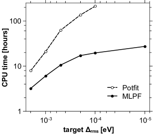
Figure 5: CPU time needed for an ML-MCTDH propagation versus the accuracy of the potential representation, for a system with 4 primitive modes. (See text for details of the system.) The open and filled circles show the timings for the potential in Potfit and MLPF representation, respectively. Data was obtained using one core of an Intel${}^{\text{\textregistered}}$ i5-3470 CPU.

target $\Delta_{\text{rms}}$ [eV]		Potfit term count		memory usage [MiB]
					Potfit		MLPF
$2\cdot 10^{-3}$		300			73		55
$1\cdot 10^{-3}$		800			121		63
$5\cdot 10^{-4}$		2299			263		74
$2\cdot 10^{-4}$		5144			533		90
$1\cdot 10^{-4}$		8044			807		105
$1\cdot 10^{-5}$							135

Table 1: Memory consumption of an ML-MCTDH propagation for a system with 4 primitive modes (see text for details), using a potential either in Potfit-format or in MLPF-format. For Potfit, the memory usage is close to proportional to the number of terms in the sum-of-products expansion.

With the potential in either Potfit- or MLPF-format, an ML-MCTDH propagation was carried out using an extended version of the Heidelberg MCTDH packagemctdh85 which can evaluate the ML-MCTDH EOMs for multi-layer operators. The initial state is described by the two molecules in their vibrational and rotational ground state, with the relative motion described by a Gaussian wavepacket centered at $R=8.0\,a_{0}$ with a width of $0.3\,a_{0}$ and a momentum of $8.0\,\hbar a_{0}^{-1}$, at zero total angular momentum. After propagating for $250\,\text{fs}$, the method of Tannor and Weekstan93:3884 was used to extract energy-resolved transition probabilities $P_{i\to f}(E)$ for rotational excitations of the molecules from the time-dependent wavefunction (see Ref. ott08:064305 for details of this analysis procedure). Here, only the four strongest rotational transitions from $i=(j_{1},j_{2})=(0,0)$ to $f=(j^{\prime}_{1},j^{\prime}_{2})=(2,0),(2,2),(4,0),(4,2)$ were considered (the $j_{i}$ are the rotational quantum numbers of the molecules; changes in the vibrational states were not considered).

Fig. 5 plots the CPU time needed for one such ML-MCTDH propagation against the target accuracy of the potential representation. (For the present system, the CPU time for producing the Potfit- and MLPF-format potentials are negligible.) As predicted, the MLPF representation shows a significantly weaker increase of the numerical effort with increasing accuracy than the Potfit representation. The computational savings factor ranges from $2.5$ to $10.8$, which roughly confirms the estimate given in Sec. V.1. Likewise, Table 1 summarizes the peak memory consumption for the ML-MCTDH propagations. Again, the resource usage is strongly reduced when using the potential in MLPF-format. For the target $\Delta_{\text{rms}}=10^{-5}\,\text{eV}$, a propagation using Potfit-format would have needed a prohibitive amount of time for the present study, and only the propagation using MLPF-format was carried out; its results were used as a reference to judge the actual accuracy of the other propagations.

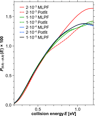
Figure 6: (color online) Convergence of the transition probability $P_{(0,0)\to(4,0)}$ with increasing accuracy of the potential representation. The legend lists the target accuracy $\Delta_{\text{rms}}$ (in eV) and the representation method. This transition was selected because it exhibits the largest deviations. Compare also with Table 2.

While Potfit and MLPF yield approximations to the potential with a controllable RMS error, the question is how the physically relevant observables are affected by these approximations. To verify that more accurate potentials indeed lead to more accurate observables, the computed transition probabilities $P_{i\to f}$ were compared to the results of the reference propagation (MLPF with $\Delta_{\text{rms}}=10^{-5}\,\text{eV}$). Among the rotational transitions considered, the one with the final state $f=(4,0)$ exhibited the most prominent differences. The convergence of the corresponding transition probabilities is displayed in Fig. 6. One can see that both Potfit and MLPF exhibit similar convergence behaviour. To make a more quantifiable statement, the following error measure can be used:

$$\text{$P$-RMSE}=\sqrt{\frac{\sum\limits_{i\to f}\,\int_{E_{0}}^{E_{1}}\!\text{d}E\left(P_{i\to f}(E)-P^{\text{ref}}_{i\to f}(E)\right)^{2}}{\sum\limits_{i\to f}^{\>}(E_{1}-E_{0})}}$$ (81)

where the integration ranges over the collision energy from $E_{0}=44\,\text{meV}$ (the energy threshold of the lowest rotational transition) to $E_{1}=1.2\,\text{eV}$, and the sum includes the four strongest rotational transitions. Table 2 shows that this error measure indeed roughly follows the accuracy of the potential representation, and that Potfit and MLPF lead to similar errors in the observables. This indicates that Potfit and MLPF lead to the same results, within the specified margin of accuracy.

target $\Delta_{\text{rms}}$ [eV]		$P$-RMSE [$10^{-3}$]
			Potfit		MLPF
$2\cdot 10^{-3}$			3.27		3.33
$1\cdot 10^{-3}$			1.39		1.98
$5\cdot 10^{-4}$			1.21		0.51
$2\cdot 10^{-4}$			0.26		0.24
$1\cdot 10^{-4}$			0.23		0.18

Table 2: Error measure (see text) of the transition probabilities $P_{i\to f}$, summed over the four strongest rotational transitions, using a potential either in Potfit- or MLPF-format. For comparison, the transition probabilities here range between $0.0$ and $0.28$, with an average value around $0.09$.

VII Summary and Outlook

While multi-layer MCTDH (ML-MCTDH) has already been successfully used for several high-dimensional systemswan03:1289; cra07:144503; wan10:78; wes11:184102; cra11:064504; ven11:044135; men12:134302; men13:014313, it has so far been difficult to use it for systems that are described by a general potential energy surface (PES). This is due to the difficulties encountered when evaluating matrix elements of the potential energy operator. The CDVR approachman96:6989; man09:054109 has been successful in overcoming these difficultiesham11:224305; ham12:054105; wes11:184102; wod12:11249; wes13:014309; wel12:244106; wel13:164118, though its use requires an enormous amount of PES evaluations, which may require a large amount of computational resources. The alternative to CDVR is to represent (or fit) the PES in a form that is compatible with ML-MCTDH, in the sense that it allows efficient evaluation of the matrix elements. Traditionally, the sum-of-products form is used, and the fitting of the PES into this form is done by the Potfit algorithmjae96:7974. However, for large systems the Potfit representation requires a huge amount of terms so that ML-MCTDH computations may become impractical.

This article has introduced the multi-layer Potfit (MLPF) method, which yields a PES representation that is as accurate as Potfit, that is as computationally affordable as Potfit, and that can reduce the computational cost for ML-MCTDH by orders of magnitude. Technically, this is achieved by employing the hierarchical singular value decompositiongra10:2029 to represent the PES in the hierarchical tensor formathac09:706 (Section IV.2). This procedure not only yields a near-optimal fit, its accuracy can also easily be estimated on the fly. Using these features, the present work shows that this algorithm can be used in a black-box-like manner, in the sense that all expansion orders could be automatically selected based on the desired root-mean-square error of the representation.

The MLPF representation of the PES allows for an efficient recursive scheme for evaluating all the ML-MCTDH matrix elements of the potential energy operator (Section III). The computational cost for this scheme has been estimated and compared to the cost induced by the Potfit representation (Section V.1). This estimate shows that MLPF can already be beneficial for systems with just four primitive modes, where computational savings of about one order of magnitude can be expected. In general, the savings are higher for more accurate representations, so that MLPF can actually yield more accurate results with less computational effort than Potfit. For a larger number of primitive modes, by using MLPF instead of Potfit, the computational effort for ML-MCTDH is expected to decrease by orders of magnitude. This means that computations once considered infeasible may now be within reach.

To test the methods discussed in this paper, an implementation of the hierarchical SVD algorithm has been written in Fortran 2003, and the Heidelberg MCTDH packagemctdh85 has been extended so that it can use the required multi-layer operator structure and treat the modified equations of motion. The code was used to study a diatom-diatom scattering system with seven degrees of freedom that are organized into four primitive modes (Section VI). Representations of the PES in Potfit- and in MLPF-format were created for different target accuracies, and an ML-MCTDH propagation with each of these PES representations was carried out. It was confirmed that Potfit and MLPF lead to the same results within the given margin of accuracy. The computational effort using the MLPF-form is indeed much lower than for the Potfit-form, especially for high-accuracy representations, where the speedup was more than a factor of ten. These results fully confirm the theoretical estimates.

The biggest limitation for MLPF is that it currently, like Potfit, needs to initially evaluate the PES on the full product grid. This limits its applicability to systems with 6–8 degrees of freedom (4–5 primitive modes). The recently introduced multigrid Potfit (MGPF) methodpel13:014108 can relax this limitation, and is easy to integrate with MLPF. This should allow treating systems with up to 12 degrees of freedom, and an example study (to be published separately) of a 9D system has so far yielded encouraging results. For larger numbers of dimensions, one must likely develop new methods for finding a good MLPF representation of the PES. As a starting point, it is worth noticing that MLPF is quite agnostic regarding the grid structure within the primitive modes. Currently, ML-MCTDH (and MLPF) can employ multi-dimensional primitive modes but requires them to use a direct product grid, so that already 3D modes become very large. Instead, one might use optimized multi-dimensional non-product grids, which will bring the modes down to a more manageable size, thus enabling the treatment of systems with a few additional degrees of freedom. Additionally, the properties of the hierarchical SVD, like giving a strict upper bound for the error, are almost too good – more approximate methods that can still work for larger systems will probably be acceptable in practice.

Appendix A Technical details of multi-layer Potfit

A.1 The MLPF algorithm

Procedures for fitting full tensors into the hierarchical tensor format have been described by Grasedyck in Ref. gra10:2029 and termed hierarchical singular value decomposition. The computationally most affordable of these algorithms is the one using leaves-to-root truncation (ibid., Algorithm 2). However, Ref. gra10:2029 (as well as other mathematical literature) only considers binary trees, whereas the trees used with ML-MCTDH may have nodes with more than two children. Hence, a minor extension of the algorithm is needed.

In the case that all leaf nodes of the ML-tree are on the same layer (i.e. they have they same distance from the top node), the MLPF algorithm proceeds as follows:

1. Obtain the potential tensor $V_{\alpha_{1}\cdots\alpha_{d}}$.

2. Use the Potfit/HOSVD algorithmjae96:7974; lat00:1253 on $V$: First, for each leaf node $z={[f]}$ …

   1. rearrange $V$ into a matrix, with $\alpha_{f}$ as the row index and all other indices combined into the column index

   2. perform a SVD of this matrix $\Rightarrow$ singular values $\sigma^{[f]}_{i}$ and left singular vectors $v^{[f]}_{i}$

   3. keep only the $m_{z}$ dominant singular vectors

   Then compute the core tensor $C$ by Eq. (66).

3. Move up one layer in the tree. If the top node is reached, the algorithm is finished. Otherwise, let there be $d^{\prime}$ nodes in this layer. For each node $z$ in this layer, combine the indices $i_{z,1},\ldots,i_{z,p_{z}}$ of its children into a multi-index $J^{z}$, so that the core tensor $C$ can be reshaped into an order-$d^{\prime}$ tensor.

4. Perform HOSVD on the reshaped $C$. This yields, for each $z$ on the current layer, singular values $\sigma^{(z)}_{i}$ (and the associated natural weights, $\lambda^{(z)}_{i}:=[\sigma^{(z)}_{i}]^{2}$) and the $m_{z}$ dominant singular vectors $v^{(z)}_{i}$. Update the core tensor by projecting the current core tensor onto outer products of the singular vectors, analogous to Eq. (66).

5. Go to step 3.

The more general case, where leaf nodes may be on different layers, can be dealt with by treating the corresponding indices of the core tensor as “by-standers”, i.e. no SVD and no projection is done along those indices, until the computation has progressed so far that the the node in question is on the current layer.

A.2 Error-controlled truncation

The error caused by MLPF can be estimated via Eq. (76). Because the natural weights are available while the algorithm progresses, one can devise a scheme which automatically chooses the truncation ranks $m_{z}$ such that the MLPF fit will have a specified accuracy. In the present work, the following scheme is used:

1. Select the desired root-mean-square (RMS) error $\Delta_{\text{rms}}$ of the MLPF representation. Set $\Delta^{2}=N_{\text{grid}}\Delta_{\text{rms}}^{2}$, where $N_{\text{grid}}$ is the number of points in the full product grid. Set $K_{\text{todo}}=K-1$. Set the current layer to the lowest layer.

2. Set $\epsilon^{2}=\Delta^{2}/K_{\text{todo}}$. Perform the HOSVD of the current layer, choosing truncation ranks $m_{z}$ such that $\sum_{i>m_{z}}\lambda^{(z)}_{i}\leq\epsilon^{2}$ for all $z$ on the current layer.

3. Update $\Delta^{2}$ by subtracting from it the sum of all neglected natural weights. Update $K_{\text{todo}}$ by subtracting from it the number of nodes on the current layer.

4. Go up one layer. If the top node is reached, exit. If there are exactly two nodes on the current layer, reduce $K_{\text{todo}}$ from 2 to 1 (because the next HOSVD will be a regular matrix SVD). Go to step 2.

Choosing the truncation ranks in this way ensures that the resulting potential approximation will have an RMS error that is not higher than $\Delta_{\text{rms}}$.

The above scheme tries to distribute the error evenly across all nodes, but if nodes on lower layers don’t use up the errors that are allocated to them, nodes on higher layers are allowed to use larger errors. This may be beneficial because it is expected that nodes closer to the top need larger truncation ranks, so this scheme helps to keep the truncation ranks more uniform. Admittedly, the given scheme is quite ad-hoc; other schemes are conceivable, e.g. one may try to distribute the error evenly across layers.

Appendix B Analysis of computational cost for ML-MCTDH

B.1 ML-MCTDH with sum-of-products operators

Let us estimate the numerical effort that is required to evaluate the ML-MCTDH EOMs with operators in sum-of-products format (see Sec. II.3). The strategy is to first compute all $\mathfrak{h}$-terms by Eq. (37), then all $\mathfrak{H}$-terms by Eq. (39), and finally the RHS of Eqs. (40–42). To illustrate how to estimate the numerical effort of these computations, take as an example the $\mathfrak{h}$-terms for a non-leaf node $z$ with $p_{z}=3$, $n_{z}=\bar{n}$, and $n_{z,\kappa}=n$, so that Eq. (37) reads

$$\mathfrak{h}^{(z)}_{r,jk} =\sum_{i_{1}=1}^{n}\sum_{i_{2}=1}^{n}\sum_{i_{3}=1}^{n}\sum_{l_{1}=1}^{n}\sum_{l_{2}=1}^{n}\sum_{l_{3}=1}^{n}A^{(z)*}_{j;i_{1}i_{2}i_{3}}A^{(z)}_{k;l_{1}l_{2}l_{3}}$$

$$\quad\times\>\mathfrak{h}^{(z,1)}_{r,i_{1}l_{1}}\mathfrak{h}^{(z,2)}_{r,i_{2}l_{2}}\mathfrak{h}^{(z,3)}_{r,i_{3}l_{3}}\quad(j,k=1\ldots\bar{n})\>.$$ (82)

In mathematical terms, $A^{(z)}_{k;l_{1}l_{2}l_{3}}$ is a tensor of order 4, and (considering only a single $r$) the $\mathfrak{h}^{(z,\kappa)}$ are matrices, and the summations over the $l_{\kappa}$ constitute matrix-tensor multiplications which can be carried out successively. The first such operation over, say, $l_{1}$ produces from $A^{(z)}$ and $\mathfrak{h}^{(z,1)}$ an intermediate order-4 tensor $X^{\prime}_{k;i_{1}l_{2}l_{3}}$. This tensor has $\bar{n}n^{3}$ elements, and each element takes $n$ FLOPs (combined floating-point multiplications and additions) to compute, leading to an overall cost of $\bar{n}n^{4}$. In the same manner, the summation over $l_{2}$ produces from $X^{\prime}$ and $\mathfrak{h}^{(z,2)}$ another intermediate tensor $X^{\prime\prime}_{k;i_{1}i_{2}l_{3}}$, which costs another $\bar{n}n^{4}$ FLOPs. Likewise for the summation over $l_{3}$, which produces a tensor $X^{\prime\prime\prime}_{k;i_{1}i_{2}i_{3}}$. Finally, the order-4 tensors $A^{(z)*}$ and $X^{\prime\prime\prime}$ are contracted over the indices $i_{1},i_{2},i_{3}$ to produce the final matrix $\mathfrak{h}^{(z)}$. This matrix has $\bar{n}^{2}$ elements, and each contraction costs $n^{3}$ FLOPs, resulting in an overall cost of $\bar{n}^{2}n^{3}$ for this last step. Hence the total cost for computing $\mathfrak{h}^{(z)}_{r,jk}$ for one $r$ and all $j,k$ is, in this specific case, $\bar{n}n^{3}(\bar{n}+3n)$, or more generally for $p_{z}=p$, $\bar{n}n^{p}(\bar{n}+pn)$. Finally, computing these terms for all $r$, i.e. for all terms in the sum-of-products expansion (32), increases the overall cost by a factor of $s$, i.e. the number of terms in this expansion.

In a similar manner, one may estimate the computational effort for the $\mathfrak{H}$-terms (39) and for the RHS of the EOMs (40–42). In case of the latter, the effort for multiplying with the inverse density matrix and for applying the projector can usually be neglected, as these need to be done only once so that their cost doesn’t depend on $s$. In summary, for a non-leaf node $z$ with $p_{z}=p$, $n_{z}=\bar{n}$, and $n_{z,\kappa}=n$, one obtains:

$$\text{cost}(\mathfrak{h}^{(z)}) =s\bar{n}n^{p}(\bar{n}+pn)$$ (83)

$$\text{cost}(\mathfrak{H}^{(z,1)})+\cdots+\text{cost}(\mathfrak{H}^{(z,p)}) =s\bar{n}n^{p}(\bar{n}+p^{2}n)$$ (84)

$$\text{cost}(\text{RHS}^{(z)}) \approx s\bar{n}n^{p}(\bar{n}+pn)$$ (85)

For leaf nodes, the computational effort depends on the sparsity of the matrix representations of the primitive mode operators, $\langle\chi^{[f]}_{\alpha}|\hat{h}^{[f]}_{r}|\chi^{[f]}_{\beta}\rangle$. If this matrix is diagonal, the effort will be proportional to $N_{f}$; for a full matrix, it is $\propto N_{f}^{2}$; if the primitive mode employs an FFT representation, the effort is $\propto N_{f}\log N_{f}$. But as was shown in section IV.1, if a general PES in Potfit form is used, most of the terms $\hat{h}^{[f]}_{r}$ have a diagonal matrix representation, and to simplify the discussion, let us assume that this is true for all terms. Then the computational effort for a leaf node $z={[f]}$ with $n_{z}=\bar{n}$ and $N_{f}=N$ becomes

$$\text{cost}(\mathfrak{h}^{(z)}) =s\bar{n}N(\bar{n}+1)$$ (86)

$$\text{cost}(\text{RHS}^{(z)}) \approx s\bar{n}N(\bar{n}+1)$$ (87)

Note that there is no equivalent of Eq. (84) for leaf nodes because they don’t have children.

To illustrate the total numerical effort for the whole ML-tree, a homogeneous tree structure like in Sec. V.1 is assumed. But here the restriction to binary trees is lifted, and more general trees with mode combinations of order $p$ are considered, so that there are $d=p^{L}$ primitive modes in the tree. As in Sec. V.1, the number of SPFs for each primitive mode is assumed to be $n$, and increases by a factor of $a$ when going one layer up. Then, summing all relevant costs from Eqs. (83–87) over all nodes, and keeping only the most expensive terms, results in:

wf-size $$\propto n^{p+1}d^{(p+1)\log_{p}a}\quad(\text{for }a>p^{1/(p+1)})$$ (88)

total-cost $$\propto s\,n^{p+2}d^{(p+2)\log_{p}a}\quad(\text{for }a>p^{1/(p+2)})$$ (89)

For $p=2$, this reproduces Manthe’s resultman08:164116 for the size of the ML-MCTDH wavefunction, but the numerical effort shows a slightly worse scaling behaviour, namely $s\,n^{4}d^{4\,log_{2}a}$. By practical experience (mostly with primitive mode combination in standard MCTDH) it was found that $a=p$ is a reasonable value, which leads to a polynomial dependence of the numerical effort on the number of degrees of freedom ($d^{4}$ for $p=2$.). However, this result is negated if $s$ has a stronger dependence on $d$, which happens to be the case if Potfit is used to represent the potential.

B.2 ML-MCTDH with multi-layer operators

Let us now estimate the numerical effort for the ML-MCTDH equations of motion in case a multi-layer operator is used. Again, the overall strategy is to first evaluate the $\mathfrak{U}$-terms (57,56), then the $\mathfrak{W}$-terms (58), and finally the RHS contributions (60–62). Naturally, the analysis of the computational costs for these expressions is now more involved.

For example, computing the $\mathfrak{U}$-terms for an internal node $z$ with $p_{z}=p$ involves an expression (cf. Eq. (56)) with 3 tensors of order $p+1$ ($V^{(z)}$, $A^{(z)*}$, $A^{(z)}$) and $p$ tensors of order 3 ($\mathfrak{U}^{(z,1)},\ldots,\mathfrak{U}^{(z,p)}$) which need to be contracted over $3p$ indices. The computational cost for this evaluation depends on the order in which the contractions are carried out, and one may attempt to find an order which minimizes this cost. This constitutes a generalization of the well-known matrix-chain multiplication problem; although the generalization to arbitrary tensors has been shown to be NP-completelam97:157, in the present case the number of tensors and contractions is small enough to make an exhaustive search feasible. Using e.g. the “single-term optimization” algorithm from Ref. har05:techrep, this search can be performed, and the results can guide the implementation. Not surprisingly, the optimal order of contractions depends on the extents of the indices involved. Moreover, the solution which minimizes the number of arithmetic operations may not be optimal in practice, as it might require an excessive amount of temporary storage (especially for larger $p_{z}$), and reducing memory consumption may anyway be beneficial on contemporary computer architectures which employ a hierarchical memory model. By considering ranges of values for $p_{z}$, $n_{z}$, $m_{z}$ which should be relevant in practice, an approach was chosen that can be implemented rather generally, that is not too far from optimal concerning computational cost, and that has moderate requirements for temporary storage.

To illustrate this approach, let us consider the $\mathfrak{U}$-terms for an internal node $z$ with $p_{z}=2$, $n_{z}=\bar{n}$, $m_{z}=\bar{m}$, $n_{z,\kappa}=n$, and $m_{z,\kappa}=m$. These terms read (cf. Eq. (56))

$$\mathfrak{U}^{(z)}_{c,jk} =\sum_{b_{1}=1}^{m}\sum_{b_{2}=1}^{m}\sum_{i_{1}=1}^{n}\sum_{i_{2}=1}^{n}\sum_{l_{1}=1}^{n}\sum_{l_{2}=1}^{n}V^{(z)}_{c;b_{1}b_{2}}$$

$$\qquad\times\>A^{(z)*}_{j;i_{1}i_{2}}A^{(z)}_{k;l_{1}l_{2}}\mathfrak{U}^{(z,1)}_{b_{1},i_{1}l_{1}}\mathfrak{U}^{(z,2)}_{b_{2},i_{2}l_{2}}$$ (90)

$$\quad(c=1\ldots\bar{m}\>;\>j,k=1\ldots\bar{n})\>.$$

First, $A^{(z)}$ is contracted with $\mathfrak{U}^{(z,1)}$ over $i_{1}$ as well as $A^{(z)*}$ with $\mathfrak{U}^{(z,2)}$ over $l_{2}$ (cost: $2m\bar{n}n^{3}$). The two resulting intermediate tensors are then contracted over $i_{2},l_{1}$ (cost: $m^{2}\bar{n}^{2}n^{2}$). The resulting tensor is finally contracted with $V^{(z)}$ over $b_{1},b_{2}$ (cost: $\bar{m}m^{2}\bar{n}^{2}$). The evaluation of the $\mathfrak{W}$-terms and the RHS contributions proceeds in a similar fashion, and the required steps have the same computational costs as those encountered for the $\mathfrak{U}$-terms.

To arrive at a cost estimate for the whole tree, consider the same homogeneous tree structure as before, but for brevity now restricted to the case $p=2$, i.e. let all $d=2^{L}$ leaf nodes employ $n$ SPFs and $m$ SPOs, and when going one layer up, let the number of SPFs and SPOs increase by a factor of $a$ and $b$, respectively (except for $n_{\varnothing}=m_{\varnothing}=1$ at the top). In general, the cost for the bottom layer can be neglected. Keeping only the highest-order terms in $n$ and $m$, one obtains (using $x^{L}=d^{\log_{2}x}$):

$$\text{node-cost}(\bar{n},n,\bar{m},m)\approx c_{1}m^{2}\bar{n}^{2}n^{2}+c_{2}\bar{m}m^{2}\bar{n}^{2}$$ (91)

(with $$c_{1} c_{2}$$, constant)

$$\text{total-cost}\approx\text{node-cost}(1,a^{L-1}n,1,b^{L-1}m)$$

$$\phantom{\text{total-cost}}+\>\sum_{l=1}^{L-1}2^{L-l}\,\text{node-cost}(a^{l}n,a^{l-1}n,b^{l}m,b^{l-1}m)$$

$$\quad\to c_{1}^{\prime}m^{2}n^{4}(a^{4}b^{2})^{L}\,+\,c_{2}^{\prime}m^{3}n^{2}(a^{2}b^{3})^{L}$$

$$\mkern 44.0mu(\text{for }L\to\infty\text{ and if }a^{4}b^{2},a^{2}b^{3}>2)$$

$$\quad\to\begin{cases}c_{1}^{\prime}m^{2}n^{4}d^{4\log_{2}a+2\log_{2}b}&\text{if }a^{2}>b\\ c_{2}^{\prime}m^{3}n^{2}d^{2\log_{2}a+3\log_{2}b}&\text{if }a^{2}<b\end{cases}$$ (92)

Assuming that $a$ and $b$ have similar values, the case $a^{2}>b$ is likely to be more relevant in practice, therefore the discussion Sec. V.1 is restricted to that case.

References