Descartes’ rule of signs and the identifiability of population demographic models from genomic variation data

Abstract

The sample frequency spectrum (SFS) is a widely-used summary statistic of genomic variation in a sample of homologous DNA sequences. It provides a highly efficient dimensional reduction of large-scale population genomic data and its mathematical dependence on the underlying population demography is well understood, thus enabling the development of efficient inference algorithms. However, it has been recently shown that very different population demographies can actually generate the same SFS for arbitrarily large sample sizes. Although in principle this nonidentifiability issue poses a thorny challenge to statistical inference, the population size functions involved in the counterexamples are arguably not so biologically realistic. Here, we revisit this problem and examine the identifiability of demographic models under the restriction that the population sizes are piecewise-defined where each piece belongs to some family of biologically-motivated functions. Under this assumption, we prove that the expected SFS of a sample uniquely determines the underlying demographic model, provided that the sample is sufficiently large. We obtain a general bound on the sample size sufficient for identifiability; the bound depends on the number of pieces in the demographic model and also on the type of population size function in each piece. In the cases of piecewise-constant, piecewise-exponential and piecewise-generalized-exponential models, which are often assumed in population genomic inferences, we provide explicit formulas for the bounds as simple functions of the number of pieces. Lastly, we obtain analogous results for the “folded” SFS, which is often used when there is ambiguity as to which allelic type is ancestral. Our results are proved using a generalization of Descartes’ rule of signs for polynomials to the Laplace transform of piecewise continuous functions.

FLA

and T1Supported in part by an NIH Grant R01-GM094402, and a Packard Fellowship for Science and Engineering.

1 Introduction

Given a sample of homologous genomic sequences from a large population, an important inference problem with a wide variety of important applications is to determine the underlying demography of the population. The population demography can be used to calibrate null models of neutral genome evolution in order to find regions under selection boyko:2008 , lohmueller:2008 , williamson:2005 ; to stratify samples in genome-wide association studies marchini:2004 , campbell:2005 , price:2006 , pasaniuc:2011 ; to date historical population splits, migrations, admixture and introgression events gravel:2011 , skoglund:2011 , li:2011 , lukic:2012 , sankararaman:2012 , kidd:2012 ; and so on. Recently, several large-sample genome- and exome-sequencing datasets have become available coventry:2010 , 1000G:2010 , nelson:2012 , tennessen:2012 , fu:2012 , shedding new light on patterns of genetic variation that were not previously observable in smaller datasets. Such large-sample studies offer an exciting opportunity to infer demography in unprecedented detail.

One widely-used measure of genetic variation in a set of homologous genome sequences is the sample frequency spectrum (SFS). For a sample of size $n$, the SFS counts the proportion of dimorphic (i.e., with exactly two distinct observed alleles) sites as a function of the frequency ($\frac{b}{n}$, where $1\leq b\leq n-1$) of the mutant allele in the sample. The SFS is useful for several reasons. First, the SFS is a succinct summary of a large sample of genomic sequences, where the information in $n$ sequences of arbitrary length can be summarized by just $n-1$ numbers. This makes the SFS both mathematically and algorithmically tractable. In particular, since the SFS ignores linkage information between sites, one can avoid challenging mathematical and computational issues associated with rigorously modeling genetic recombination. Furthermore, the statistical properties of the SFS and their dependence on the population demographic history are well understood under the coalescent and the diffusion models of neutral evolution kimura:1955 , fu:1995 , griffiths:1998 , griffiths:2003 , polanski:2003 , zivkovic:2011 . This dependence of the SFS on demography, along with the assumption of free recombination between sites, has been exploited in several efficient methods for inferring historical population demography marth:2004 , gutenkunst:2009 , lukic:2011 , excoffier:2013 . Second, the SFS can effectively capture the impact of recent demography on genetic variation. Recent large-sample studies coventry:2010 , nelson:2012 , tennessen:2012 , fu:2012 have consistently shown that there is an excess of rare polymorphisms compared to the predictions of previously inferred demographic models, which might be explained by recent rapid population expansion keinan:2012 . Because the leading entries of the SFS count the rare variants in the sample, one might be able to use this information to infer demographic events in the recent past at a much finer resolution than possible using smaller samples. Third, the SFS also provides a simple way of visualizing the goodness of fit of a demographic model to data, since one can easily compare the SFS observed in the data with the SFS predicted by the fitted demographic model.

While the SFS has algorithmic advantages for demographic inference, it is believed to suffer from a statistical shortcoming. Specifically, Myers, Fefferman and Patterson myers:2008 recently showed that even with perfect knowledge of the population frequency spectrum [i.e., the proportion of polymorphic sites with population-wide allele frequency in $(x,x+dx)$ for all $x\in(0,1)$], the historical population size function $\eta(t)$ as a function of time is not identifiable. Using Müntz–Szász theory, they showed that for any population size function $\eta(t)$, one can construct arbitrarily many smooth functions $F(t)$ such that both $\eta(t)$ and $\eta(t)+\alpha F(t)$ generate the same population frequency spectrum for suitably chosen values of $\alpha$. They also constructed explicit examples of such functions $\eta(t)$ and $F(t)$. While this nonidentifiability could pose serious challenges to demographic inference from frequency spectrum data, the population size functions involved in their example are arguably unrealistic for biological populations. In particular, their explicit example involves a population size function which oscillates at an increasingly higher frequency as the time parameter approaches the present. Real biological population sizes can be expected to vary over time in a mathematically more well-behaved fashion. In particular, populations can be expected to evolve in discrete units of time, which, when approximated by a continuous-time model, restricts the frequency of oscillations in the population size function to be less than the number of generations of reproduction per unit time. Furthermore, since a population size model being inferred must have a finite representation for obvious algorithmic reasons, most previous demographic inference analyses have focused on inferring population size models that are piecewise-defined over a restricted class of functions, such as piecewise-constant and piecewise-exponential models schaffner:2005 , keinan:2007 , li:2011 , gravel:2011 , lukic:2012 , nelson:2012 , tennessen:2012 . Motivated by the large number of rare variants observed in several large-sample sequencing studies, recent works reppell:2012 , reppell:2013 have also focused on more general population growth models which allow for the population to grow at a faster than exponential rate. Each piece in such piecewise models has two parameters that control the rate and acceleration of population growth. Since these models contain the family of piecewise-constant and piecewise-exponential population size functions, we refer to them as piecewise-generalized-exponential models in the remainder of this paper.

In this paper, we revisit the question of demographic model identifiability under the assumption that the population size is a piecewise-defined function of time where each piece comes from a family of biologically-motivated functions, such as the family of constant or exponential functions. We also re-examine the assumption that one has access to the population-wide patterns of polymorphism. In real applications, we do not expect to know the allele frequency spectrum for an entire population but rather only the SFS for a randomly drawn finite sample of individuals. Here, we investigate whether one can learn piecewise-defined population size functions given perfect knowledge of the expected SFS for a sufficiently large sample of size $n$. Unlike in the case of arbitrary continuous population size functions considered by Myers, Fefferman and Patterson, the answer to this question is affirmative. More precisely, we obtain bounds on the sample size $n$ that are sufficient to distinguish population size functions among piecewise demographic models with $K$ pieces, where each piece comes from some family of functions (see Theorems 6 and 11). Our bound on the sample size can be expressed as an affine function of the number $K$ of pieces, where the slope of the function is a measure of the complexity of the family to which each piece belongs. In the cases of piecewise-constant, piecewise-exponential and piecewise-generalized-exponential models, which are often assumed in population genetic analyses, the slope of this affine function can be calculated explicitly, as shown in Corollaries 7–9. We also obtain analogous results for the “folded” SFS (see Theorem 12), a variant of the SFS which circumvents the ambiguity in the identity of the ancestral allele type by grouping the polymorphic sites in a sample according to the sample minor allele frequency.

There are two main technical elements underlying our proofs of the identifiability results mentioned above. The first step is to show that the expected SFS of a sample of size $n$ is in bijection with the Laplace transform of a time-rescaled version of the population size function evaluated at a particular sequence of $n-1$ points. This reduces the problem of identifiability from the SFS to that of identifiability from the values of the Laplace transform at a fixed set of points. The second step relies on a generalization of Descartes’ rule of signs for polynomials to the Laplace transform of general piecewise-continuous functions. This technique yields an upper bound on the number of roots of the Laplace transform of a function by the number of sign changes of the function. We think that this proof technique based on sign changes might be of independent interest for proving statistical identifiability results in other settings. We also provide an alternate proof of identifiability for piecewise-constant population models, where the aforementioned second step is replaced by a linear algebraic argument that has a constructive flavor. We include this alternate proof in the hope that it could be used to develop an algebraic inference algorithm for piecewise-constant models.

The remainder of this paper is organized as follows. In Section 2, we introduce the model and notation, and describe our main results. We also discuss the counterexample of Myers, Fefferman and Patterson in light of our findings. The proofs of our results are provided in Section 3, and we conclude with a discussion in Section 4.

2 Main results

Here, we summarize our identifiability results. All proofs are deferred to Section 3.

2.1 Model and notation

We consider a population evolving according to Kingman’s coalescent kingman:1982:SPA , kingman:1982:JAP , kingman:1982:EPS with the infinite-sites model of mutation kimura:1969 and selective neutrality. Under this model, the genome is assumed to be infinite and every mutation occurs at a different site in the genome that has never experienced a mutation before. This model is applicable in the regime where the mutation rate is very low, and hence the probability of multiple mutations at a given site is vanishingly small. Any polymorphic site in a sample of sequences is dimorphic under this model. The population size is assumed to change deterministically with time and is described by a function $\eta\dvtx\mathbb{R}_{\geq 0}\to\mathbb{R}_{+}$, such that the instantaneous coalescence rate between any pair of lineages at time $t$ is $1/\eta(t)$.

Let $T^{(\eta)}_{n,k}$ denote the time (in coalescent units) while there are $k$ ancestral lineages for a sample of size $n$ obtained at time $0$. Defining $R_{\eta}(t)$ as

$$R_{\eta}(t):=\int_{0}^{t}\frac{1}{\eta(x)}\,dx,$$

the expected time $\mathbb{E}[T^{(\eta)}_{m,m}]$ to the first coalescence event for a sample of size $m$ is given by

$$\mathbb{E}\bigl{[}T^{(\eta)}_{m,m}\bigr{]}=\int_{0}^{\infty}t\frac{{m\choose 2}}{\eta(t)}\exp\biggl{[}-\pmatrix{m\cr 2}R_{\eta}(t)\biggr{]}\,dt.$$ (1)

Following the notation of Myers, Fefferman and Patterson, define a time-rescaled version $\widetilde{\eta}$ of the population size function $\eta$ as

$$\widetilde{\eta}(\tau)=\eta\bigl{(}R_{\eta}^{-1}(\tau)\bigr{)},$$ (2)

where $\tau\in\mathbb{R}_{\geq 0}$. The function $\widetilde{\eta}(\tau)$ reparameterizes the population size as a function of the cumulative rate of coalescence $\tau=R_{\eta}(t)$. For a given population size function $\widetilde{\eta}$ parameterized by the total coalescence rate $\tau$, there corresponds a unique population size function $\eta$ parameterized by time $t$. Specifically, $\eta(t)=\widetilde{\eta}(S_{\widetilde{\eta}}^{-1}(t))$, for all $t\in\mathbb{R}_{\geq 0}$, where $S_{\widetilde{\eta}}(t)$ is an invertible function given by

$$S_{\widetilde{\eta}}(t)=\int_{0}^{t}\widetilde{\eta}(x)\,dx.$$

Applying integration by parts to (1) and using the condition that $\mathbb{E}[T^{(\eta)}_{m,m}]<\infty$, we have

$$\mathbb{E}\bigl{[}T^{(\eta)}_{m,m}\bigr{]}=\int_{0}^{\infty}\exp\biggl{[}-\pmatrix{m\cr 2}R_{\eta}(t)\biggr{]}\,dt.$$ (3)

Furthermore, since $R_{\eta}$ is monotonically increasing and continuous from $\mathbb{R}_{\geq 0}$ to $\mathbb{R}_{\geq 0}$, it is a bijection over $\mathbb{R}_{\geq 0}$. For notational convenience, for any interval $I\subseteq\mathbb{R}_{\geq 0}$, we define $R_{\eta}(I)$ to be the interval

$$R_{\eta}(I)=\bigl{\{}R_{\eta}(x)|x\in I\bigr{\}}.$$

By making the substitution $\tau=R_{\eta}(t)$ in (3) and using (2), we have the following expression for $\mathbb{E}[T^{(\eta)}_{m,m}]$:

$$\mathbb{E}\bigl{[}T^{(\eta)}_{m,m}\bigr{]}=\int_{0}^{\infty}\widetilde{\eta}(\tau)\exp\biggl{[}-\pmatrix{m\cr 2}\tau\biggr{]}\,d\tau.$$ (4)

Equation (4) states that the time to the first coalescence event for a sample of size $m$ is given by the Laplace transform of the time-rescaled population size function $\widetilde{\eta}$ evaluated at the point ${m\choose 2}$. For a sample of size $n$, let $\xi_{n,b}$ denote the probability that a dimorphic site has $b$ mutant alleles and $n-b$ ancestral alleles. We refer to $(\xi_{n,1},\ldots,\xi_{n,n-1})$ as the expected sample frequency spectrum (SFS).

2.2 Determining the expected times to the first coalescence from the SFS

The following lemma shows that the expected SFS for a sample of size $n$ tightly constrains the expected time to the first coalescence event for all sample sizes $2,\ldots,n$:

Lemma 1.

Under an arbitrary variable population size model $\{\eta(t),t\geq 0\}$, suppose $\xi_{n,1},\ldots,\xi_{n,n-1}$ are known and define $c_{m}:=\mathbb{E}[T^{(\eta)}_{m,m}]$ for $2\leq m\leq n$. Then, up to a common positive multiplicative constant, the quantities $c_{2},\ldots,c_{n}$ can be determined uniquely from $\xi_{n,1},\ldots,\xi_{n,n-1}$.

This implies that the problem of identifying the population size function $\eta(t)$ from $\xi_{n,1},\ldots,\xi_{n,n-1}$ can be reduced, up to a multiplicative constant, to the problem of identifying $\eta(t)$ from $c_{2},\ldots,c_{n}$.

2.3 Piecewise population size models and sign change complexities

To state our main result in full generality, we first need a few definitions.

Definition 1 ((${\mathcal{F}}$, family of continuous population size functions)).

A family ${\mathcal{F}}$ of continuous population size functions is a set of positive continuous functions $f\dvtx\mathbb{R}_{\geq 0}\to\mathbb{R}_{+}$ of a particular type parameterized by a collection of variables.

We use ${\mathcal{F}}_{c}$ to denote the family of constant population size functions; that is, functions of the form $f(t)=\nu$ for all $t$, where $\nu\in\mathbb{R}_{+}$ is the only parameter of the family. Further, we use ${\mathcal{F}}_{e}$ to denote the family of exponential population size functions of the form $f(t)=\nu\exp(\beta t)$, where $\nu\in\mathbb{R}_{+}$ and $\beta\in\mathbb{R}$ are the parameters of the family. In human genetics, there has been recent interest reppell:2012 , reppell:2013 in modeling superexponential growth in the effective population size via models that generalize exponential growth by incorporating an additional acceleration parameter $\gamma$. Such population size functions $f$ satisfy the differential equation $df/dt=\beta f(t)^{\gamma}$ with initial condition $f(0)=\nu$, where $\beta\in\mathbb{R},\gamma\in\mathbb{R}_{\geq 0}$, and $\nu\in\mathbb{R}_{+}$. When $0\leq\gamma<1$ (resp., $\gamma>1$), this represents superexponential (resp., subexponential) population growth/decline, while $\gamma=1$ corresponds to exponential population growth/decline. We let ${\mathcal{F}}_{g}$ denote the family of such generalized-exponential population size functions.

Definition 2 ([${\mathcal{M}}_{K}({\mathcal{F}})$, piecewise models over ${\mathcal{F}}$ with at most $K$ pieces]).

Given a family ${\mathcal{F}}$ of continuous population size functions, a population size function $\eta(t)$ defined over $\mathbb{R}_{\geq 0}$ is said to be piecewise over ${\mathcal{F}}$ with at most $K$ pieces if there exists an integer $p$, where $1\leq p\leq K-1$, and a sequence of $p$ time points $0<t_{1}<\cdots<t_{p}<\infty$ such that for each $1\leq i\leq p+1$, there exists a positive continuous function $f_{i}\in{\mathcal{F}}$ such that $\eta(t)=f_{i}(t-t_{i-1})$ for all $t\in[t_{i-1},t_{i})$. For convention, we define $t_{0}=0$ and $t_{p+1}=\infty$. Note that $\eta$ may not be continuous at the change points $t_{1},\ldots,t_{p}$. We use ${\mathcal{M}}_{K}({\mathcal{F}})$ to denote the space of such piecewise population size models with at most $K$ pieces, each of which belongs to function family ${\mathcal{F}}$. Illustrated in Figure 1 is an example of piecewise-exponential population size function $\eta\in{\mathcal{M}}_{K}({\mathcal{F}})$ where $K\geq 5$ and ${\mathcal{F}}={\mathcal{F}}_{e}$.

Definition 3 ([$\sigma(f)$, number of sign changes of a function]).

For a function $g$ (not necessarily continuous) defined over some interval $(a,b)$, we say that $t\in(a,b)$ is a sign change point of $g$ if there exist some $\varepsilon>0$, $t^{\prime}\geq t$, and an interval $(t^{\prime},t^{\prime}+\varepsilon)\subseteq(a,b)$ such that: [1.]

$(t-\varepsilon,t)\subseteq(a,b)$,

$g(z)=0$ for $z\in(t,t^{\prime})$,

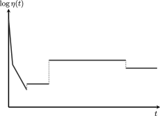
Figure 1: A piecewise-exponential population size function $\eta\in{\mathcal{M}}_{K}({\mathcal{F}}_{e})$, where $K\geq 5$. Note that the $y$-axis is in a log scale. This piecewise-exponential function depicts the historical population size changes of a European population that was estimated from the SFS of a sample of $1351$ (diploid) individuals of European ancestry tennessen:2012 .

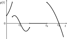
Figure 2: Illustration of the sign changes of a function. For the domain shown, $\sigma(g)=3$ and the sign change points of $g$ are denoted $t_{1},t_{2}$, and $t_{3}$.

$g(x)g(y)<0$ for all $x\in(t-\varepsilon,t)$ and $y\in(t^{\prime},t^{\prime}+\varepsilon)$. We define the number $\sigma(g)$ of sign changes of $g$ as the number of such sign change points in its domain $(a,b)$. See Figure 2 for an illustration.

Note that the above definition of the number of sign changes counts the number of times the function $g$ changes value from positive to negative (and vice versa) while ignoring intervals where it is identically zero. While the above definition is not restricted to piecewise continuous functions, we will restrict our attention to such functions for the remainder of this paper.

Definition 4 ([$\mathscr{S}({\mathcal{F}})$ and $\mathscr{S}({\mathcal{M}}_{K}({\mathcal{F}}))$, sign change complexities]).

For a family ${\mathcal{F}}$ of continuous population size functions, we define the sign change complexity $\mathscr{S}({\mathcal{F}})$ as

$$\mathscr{S}({\mathcal{F}}) = \mathop{\sup_{f_{1},f_{2}\in{\mathcal{F}},}}_{a_{1},a_{2}\in\mathbb{R}_{\geq 0}}\left\{\sigma(g)\Bigg{|}\begin{array}[]{l}g(\tau):=\widetilde{f}_{1}(\tau-a_{1})-\widetilde{f}_{2}(\tau-a_{2})\mbox{ with domain }\\ \operatorname{Dom}(g)=\biggl{\{}\tau\in\mathbb{R}_{\geq 0}\bigg{|}\begin{array}[]{l}\tau-a_{1}\in\operatorname{Dom}(\widetilde{f}_{1}),\\ \tau-a_{2}\in\operatorname{Dom}(\widetilde{f}_{2})\end{array}\biggr{\}}\end{array}\right\}$$ (9)

$$= \mathop{\sup_{f_{1},f_{2}\in{\mathcal{F}},}}_{a\in\mathbb{R}_{\geq 0}}\left\{\sigma(g)\Bigg{|}\begin{array}[]{l}g(\tau):=\widetilde{f}_{1}(\tau)-\widetilde{f}_{2}(\tau-a)\mbox{ with domain }\\ \operatorname{Dom}(g)=\biggl{\{}\tau\in\mathbb{R}_{\geq 0}\bigg{|}\begin{array}[]{l}\tau\in\operatorname{Dom}(\widetilde{f}_{1}),\\ \tau-a\in\operatorname{Dom}(\widetilde{f}_{2})\end{array}\biggr{\}}\end{array}\right\},$$ (15)

where $\widetilde{f}_{j}$ are the time-rescaled versions of $f_{j}$ as defined in (2), and $\operatorname{Dom}(\widetilde{f}_{j})=R_{f_{j}}(\mathbb{R}_{\geq 0})$ is the domain of $\widetilde{f}_{j}$. Similarly, for the space ${\mathcal{M}}_{K}({\mathcal{F}})$ of piecewise population size models with at most $K$ pieces over some function family ${\mathcal{F}}$, we define the sign change complexity $\mathscr{S}({\mathcal{M}}_{K}({\mathcal{F}}))$ as

$$\mathscr{S}\bigl{(}{\mathcal{M}}_{K}({\mathcal{F}})\bigr{)}=\sup_{\eta_{1},\eta_{2}\in{\mathcal{M}}_{K}({\mathcal{F}})}\bigl{\{}\sigma(\widetilde{\eta}_{1}-\widetilde{\eta}_{2})\bigr{\}},$$

where, again, $\widetilde{\eta}_{j}$ are related to $\eta_{j}$ as given in (2).

The following lemma gives a bound on the sign change complexity of a model with at most $K$ pieces in terms of the underlying family of population size functions for each piece.

Lemma 2.

The sign change complexity of the space ${\mathcal{M}}_{K}({\mathcal{F}})$ of piecewise models with at most $K$ pieces in a function family ${\mathcal{F}}$ is bounded by the sign change complexity of ${\mathcal{F}}$ as

$$\mathscr{S}\bigl{(}{\mathcal{M}}_{K}({\mathcal{F}})\bigr{)}\leq(2K-2)+(2K-1)\mathscr{S}({\mathcal{F}}).$$

Note that the bound in Lemma 2 is tight for the family ${\mathcal{F}}_{c}$ of constant population sizes, for which $\mathscr{S}({\mathcal{F}}_{c})=0$ and $\mathscr{S}({\mathcal{M}}_{K}({\mathcal{F}}_{c}))=2K-2$.

2.4 Identifiability results

Our main results on identifiability will be proved using a generalization of Descartes’ rule of signs for polynomials.

Theorem 3 ((Descartes’ rule of signs for polynomials))

Consider a degree-$n$ polynomial $p(x)=a_{0}+a_{1}x+\cdots+a_{n}x^{n}$ with real-valued coefficients $a_{i}$. The number of positive real roots (counted with multiplicity) of $p$ is at most the number of sign changes between consecutive nonzero terms in the sequence $a_{0},a_{1},\ldots,a_{n}$.

The following theorem generalizes the above classic result to relate the number of sign changes of a piecewise-continuous function $f$ to the number of roots of its Laplace transform.

Theorem 4 ((Generalized Descartes’ rule of signs))

Let $f\dvtx\mathbb{R}_{\geq 0}\to\mathbb{R}$ be a piecewise-continuous function which is not identically zero and with a finite number $\sigma(f)$ of sign changes. Then the function $G(x)$ defined by

$$G(x)=\int_{0}^{\infty}f(t)e^{-tx}\,dt$$ (16)

has at most $\sigma(f)$ roots in $\mathbb{R}$ (counted with multiplicity).

The statement of Theorem 4 and the proof provided in Section 3 are adapted from Jameson jameson:2006 , Lemma 4.5, for our setting. Using Theorem 4, we prove in Section 3 the following identifiability theorem for population size function families with finite sign change complexity.

Theorem 5

For a sample of size $n$, let $\mathbf{c}=(c_{2},\ldots,c_{n})$, where $c_{m}=\mathbb{E}[T^{(\eta)}_{m,m}]$, for $2\leq m\leq n$, defined in (3). If $\mathscr{S}({\mathcal{F}})<\infty$ and $n\geq\mathscr{S}({\mathcal{F}})+2$, then no two distinct models $\eta_{1},\eta_{2}\in{\mathcal{F}}$ can produce the same $(c_{2},\ldots,c_{n})$. In other words, for $n\geq\mathscr{S}({\mathcal{F}})+2$, the map $\mathbf{c}\dvtx{\mathcal{F}}\to\mathbb{R}_{+}^{n-1}$ is injective.

Note that the sample size bound in Theorem 5 applies to an arbitrary function family ${\mathcal{F}}$ which need not have any special structure. Using Lemma 2 for bounding the sign change complexity of piecewise-defined function families ${\mathcal{M}}_{K}({\mathcal{F}})$ in terms of the sign change complexity of the underlying function family ${\mathcal{F}}$, we immediately obtain the following theorem.

Theorem 6

For a sample of size $n$, let $\mathbf{c}=(c_{2},\ldots,c_{n})$, where $c_{m}=\mathbb{E}[T^{(\eta)}_{m,m}]$, for $2\leq m\leq n$, defined in (3). If $\mathscr{S}({\mathcal{F}})<\infty$ and $n\geq 2K+(2K-1)\mathscr{S}({\mathcal{F}})$, then the map $\mathbf{c}\dvtx{\mathcal{M}}_{K}({\mathcal{F}})\to\mathbb{R}_{+}^{n-1}$ is injective.

Using Theorem 6, it is simple to derive identifiability results for piecewise-defined population size models over several function families ${\mathcal{F}}$ that are of biological interest. In particular, we have the following result for the case of piecewise-constant models.

Corollary 7 ([Identifiability of piecewise-constant population size models in ${\mathcal{M}}_{K}({\mathcal{F}}_{c})$]).

The map $\mathbf{c}\dvtx{\mathcal{M}}_{K}({\mathcal{F}}_{c})\to\mathbb{R}_{+}^{n-1}$ is injective if the sample size $n\geq 2K$.

The bound in Corollary 7 on the sample size sufficient for identifying piecewise-constant population models is actually tight, since ${\mathcal{M}}_{K}({\mathcal{F}}_{c})$ has $2K-1$ parameters in $\mathbb{R}_{+}$ and there is no continuous injective function from $\mathbb{R}_{+}^{2K-1}$ to $\mathbb{R}^{n-1}$ if $n<2K$. (This fact can be proved in multiple ways, such as by the Borsuk–Ulam theorem or the Constant Rank theorem.) An alternate proof of Corollary 7 that does not rely on Theorem 6 is also provided in Section 3. This alternate proof is based on an argument from linear algebra, and it might be possible to adapt this approach to develop an algebraic algorithm for inferring the parameters of a piecewise-constant population function from the set of expected first coalescence times $c_{m}$.

Another class of models often assumed in population genetic analyses are piecewise-exponential functions, for which we have the following result.

Corollary 8 ([Identifiability of piecewise-exponential population size models in ${\mathcal{M}}_{K}({\mathcal{F}}_{e})$]).

The map $\mathbf{c}\dvtx{\mathcal{M}}_{K}({\mathcal{F}}_{e})\to\mathbb{R}_{+}^{n-1}$ is injective if the sample size $n\geq 4K-1$.

For the generalized-exponential growth models considered by Reppell, Boehnke and Zöllner reppell:2013 , we have the following result.

Corollary 9 ([Identifiability of piecewise-generalized-exponential population size models in ${\mathcal{M}}_{K}({\mathcal{F}}_{g})$]).

The map $\mathbf{c}\dvtx{\mathcal{M}}_{K}({\mathcal{F}}_{g})\to\mathbb{R}_{+}^{n-1}$ is injective if the sample size $n\geq 6K-2$.

For the identifiability of piecewise population size models from the SFS data, we first note the following lemma.

Lemma 10.

Consider a piecewise population size function $\eta\in{\mathcal{M}}_{K}({\mathcal{F}})$. Consider a sample of size $n\geq 2K+(2K-1)\mathscr{S}({\mathcal{F}})$ and suppose the function $\eta$ produces $\mathbb{E}[T^{(\eta)}_{m,m}]=c_{m}$ for $2\leq m\leq n$. Then, for every fixed $\kappa\in\mathbb{R}_{+}$, there exists a unique piecewise population size function $\zeta\in{\mathcal{M}}_{K}({\mathcal{F}})$ with $\mathbb{E}[T^{(\zeta)}_{m,m}]=\kappa c_{m}$ for $2\leq m\leq n$. Furthermore, this population size function $\zeta$ is given by $\zeta(t)=\kappa\eta(t/\kappa)$.

Given two models $\eta,\zeta\in{\mathcal{M}}_{K}$, we say that $\eta$ and $\zeta$ are equivalent, and write $\eta\sim\zeta$, if they are related by a rescaling of change points and population sizes as described in Lemma 10. Let $[\eta]$ denote the equivalence class of population size functions that contain $\eta$, and let ${\mathcal{M}}_{K}({\mathcal{F}})/{\sim}{}=\{[\eta]|\eta\in{\mathcal{M}}_{K}({\mathcal{F}})\}$ be the set of equivalence classes for the equivalence relation $\sim$. Then, combining Lemma 1, Theorem 6 and Lemma 10, we obtain the following theorem.

Theorem 11

If $\mathscr{S}({\mathcal{F}})<\infty$ and $n\geq 2K+(2K-1)\mathscr{S}({\mathcal{F}})$, then, for each expected SFS $(\xi_{n,1},\ldots,\xi_{n,n-1})$, there exists a unique equivalence class $[\eta]$ of models in ${\mathcal{M}}_{K}({\mathcal{F}})/{\sim}$ consistent with $(\xi_{n,1},\ldots,\xi_{n,n-1})$.

2.5 Extension to the folded frequency spectrum

To generate the SFS from genomic sequence data, one needs to know the identities of the ancestral and mutant alleles at each site. To avoid this problem, a commonly employed strategy in population genetic inference involves “folding” the SFS. More precisely, for a sample of size $n$, the $i$th entry of the folded SFS $\bolds{\chi}=(\chi_{n,1},\ldots,\chi_{\lfloor{n}/{2}\rfloor})$ is defined by

$$\chi_{n,i}=\frac{\xi_{n,i}+\xi_{n,n-i}}{1+\delta_{i,n-i}},$$

where $1\leq i\leq\lfloor{n}/{2}\rfloor$. In particular, $\chi_{n,i}$ is the proportion of polymorphic sites that have $i$ copies of the minor allele. For any sample size $n$, since $\mathbf{\chi}$ is a vector of approximately half the dimension as $\bolds{\xi}$, we might expect to require roughly twice as many samples to recover the demographic model from $\bolds{\chi}$ compared to $\bolds{\xi}$. This is indeed the case. Given the folded SFS $\bolds{\chi}$, the following theorem establishes a sufficiency condition on the sample size for identifying demographic models in ${\mathcal{M}}_{K}({\mathcal{F}})$.

Theorem 12

If $\mathscr{S}({\mathcal{F}})<\infty$ and $n\geq 2(2K-1)(1+\mathscr{S}({\mathcal{F}}))$, then, for each expected folded SFS $\bolds{\chi}=(\chi_{n,1},\ldots,\chi_{n,{\lfloor{n}/{2}\rfloor}})$, there exists a unique equivalence class $[\eta]$ of models in ${\mathcal{M}}_{K}({\mathcal{F}})/{\sim}$ consistent with $\bolds{\chi}$.

2.6 The counterexample of Myers, Fefferman and Patterson

Myers, Fefferman and Patterson myers:2008 provided an explicit counterexample to the identifiability of population size models from the allelic frequency spectrum. In our notation, they provided two time-rescaled population size functions $\widetilde{\eta}_{1}$ and $\widetilde{\eta}_{2}$ given by

$$\widetilde{\eta}_{1}(\tau) = N,$$

$$\widetilde{\eta}_{2}(\tau) = N\bigl{(}1-9F(\tau)\bigr{)},$$

where $N$ is an arbitrary positive constant, and the function $F$ is given by the convolution

$$F(\tau)=\int_{0}^{\tau}f_{0}(\tau-u)f_{1}(u)\,du,$$

where $f_{0}$ and $f_{1}$ are given by

$$f_{0}(\tau) = \exp\bigl{(}-1/\tau^{2}\bigr{)},$$

$$f_{1}(\tau) = \frac{\cos(\pi^{2}/\tau)\exp(-\tau/8)}{\sqrt{\tau}}.$$

Both functions $f_{1}$ and $F$ have increasingly frequent oscillations as $\tau\downarrow 0$ so that $\sigma(\widetilde{\eta}_{1}-\widetilde{\eta}_{2})=\sigma(F)=\infty$. This is why Theorem 5 does not apply to this example. Indeed, by an argument using the Laplace transforms of $f_{1}$ and $F$, Myers, Fefferman and Patterson showed that the function $G(x)$ defined in (16) in terms of $F$ has roots at $-{m\choose 2}$ for each $m\geq 2$.

3 Proofs

We now provide proofs of the results presented earlier.

Proof of Lemma 1 In the coalescent for a sample of size $n$, let $\gamma_{n,b}$ denote the total expected branch length subtending $b$ leaves, for $1\leq b\leq n-1$. Then $\xi_{n,b}=\gamma_{n,b}/\sum_{k=1}^{n-1}\gamma_{n,k}$, which implies that there exists a positive constant $\kappa$ such that $\gamma_{n,b}=\kappa\xi_{n,b}$ for all $1\leq b\leq n-1$. We now prove that $c_{2},\ldots,c_{n}$ can be determined uniquely from $\gamma_{n,1},\ldots,\gamma_{n,n-1}$.

Let $\phi_{n,k}=\mathbb{E}[T^{(\eta)}_{n,k}]$. Then, by a result of Griffiths and Tavaré griffiths:1998 ,

$$\gamma_{n,b}=\sum_{k=2}^{n-b+1}k\frac{{n-b-1\choose k-2}}{{n-1\choose k-1}}\phi_{n,k},$$ (17)

for $1\leq b\leq n-1$. The system of equations (17) can be rewritten succinctly as a linear system

$$\bolds{\gamma}=\mathbf{M}\bolds{\phi},$$

where $\bolds{\gamma}=(\gamma_{n,1},\ldots,\gamma_{n,n-1})$, $\mathbf{\phi}=(\phi_{n,2},\ldots,\phi_{n,n})$, and $\mathbf{M}=(m_{bk})$ with $m_{bk}=k{{n-b-1\choose k-2}}/{{n-1\choose k-1}}$, for $1\leq b\leq n-1$ and $2\leq k\leq n$. The matrix $\mathbf{M}$ is upper-left triangular since ${n-b-1\choose k-2}=0$ if $k>n-b+1$, and the anti-diagonal entries are $\frac{k}{{n-1\choose k-1}}>0$. Hence, $\det(\mathbf{M})\neq 0$ and $\mathbf{M}$ is therefore invertible. Thus, given $\bolds{\gamma}$, we can determine $\bolds{\phi}$ uniquely as $\mathbf{M}^{-1}\bolds{\gamma}$.

Let $\psi_{n,k}=\sum_{j=k}^{n}{\mathbb{E}[T^{(\eta)}_{n,j}]}$. Then, defining $\psi_{n,n+1}:=0$, observe that $\psi_{n,k}=\phi_{n,k}+\psi_{n,k+1}$ for $2\leq k\leq n$. This implies that $\psi_{n,2},\ldots,\psi_{n,n}$ can be determined uniquely from $\phi_{n,2},\ldots,\phi_{n,n}$. Polanski, Bobrowski and Kimmel polanski:2003 showed that $\psi_{n,k}$ can be written as

$$\psi_{n,k}=\sum_{m=k}^{n}a_{km}c_{m},$$ (18)

where $a_{km}$, for $k\leq m\leq n$, are given by

$$a_{km}=\frac{\prod_{l=k,l\neq m}^{n}{l\choose 2}}{\prod_{l=k,l\neq m}^{n}[{l\choose 2}-{m\choose 2}]},$$

and $c_{m}=\mathbb{E}[T^{(\eta)}_{m,m}]$, shown in (3). Again, the system of equations (18) can be written as a triangular linear system

$$\bolds{\psi}=\mathbf{A}\mathbf{c},$$

where $\bolds{\psi}=(\psi_{n,2},\ldots,\psi_{n,n})$, $\mathbf{c}=(c_{2},\ldots,c_{n})$, and $\mathbf{A}=(a_{km})$, for $2\leq k,m\leq n$. Note that $\mathbf{A}$ is an upper triangular matrix since $a_{km}:=0$ if $m<k$. Since $\mathbf{A}$ has nonzero entries on its diagonal, $\mathbf{A}^{-1}$ exists, and $\mathbf{c}$ can be determined uniquely as $\mathbf{A}^{-1}\bolds{\psi}$.

Proof of Lemma 2 Given a pair of piecewise population size functions $\eta_{1},\eta_{2}\in{\mathcal{M}}_{K}({\mathcal{F}})$, let $\widetilde{\eta}_{1}$ and $\widetilde{\eta}_{2}$ be their respective time-rescaled versions, defined by (2). Let $0<t^{(1)}_{1}<\cdots<t^{(1)}_{p_{1}}<\infty$, where $0\leq p_{1}\leq K-1$ (resp., $0<t^{(2)}_{1}<\cdots<t^{(2)}_{p_{2}}<\infty$, where $0\leq p_{2}\leq K-1$) be the change points of the pieces of $\eta_{1}$ (resp., $\eta_{2}$). We define $t^{(1)}_{0}=t^{(2)}_{0}=0$ and $t^{(1)}_{p_{1}+1}=t^{(2)}_{p_{2}+1}=\infty$. The change points of $\widetilde{\eta}_{1}$ are given by $R_{\eta_{1}}(t^{(1)}_{i})$, where $1\leq i\leq p_{1}$, while the change points of $\widetilde{\eta}_{2}$ are given by $R_{\eta_{2}}(t^{(2)}_{i})$, where $1\leq i\leq p_{2}$. Let $0<\tau_{1}<\cdots<\tau_{p}<\infty$ be the union of the change points of $\widetilde{\eta}_{1}$ and $\widetilde{\eta}_{2}$, where $0\leq p\leq p_{1}+p_{2}$. For convention, let $\tau_{0}=0$ and $\tau_{p+1}=\infty$.

Consider the piece $(\tau_{i},\tau_{i+1})$ for $0\leq i\leq p$. Let $I_{1}=(t^{(1)}_{k},t^{(1)}_{k+1})$, where $0\leq k\leq p_{1}$, and $I_{2}=(t^{(2)}_{l},t^{(2)}_{l+1})$, where $0\leq l\leq p_{2}$, be the pieces of the original population size functions $\eta_{1}$ and $\eta_{2}$, respectively, such that $(\tau_{i},\tau_{i+1})\subseteq R_{\eta_{1}}(I_{1})$ and $(\tau_{i},\tau_{i+1})\subseteq R_{\eta_{2}}(I_{2})$. Since $\eta_{1}\in{\mathcal{M}}_{K}({\mathcal{F}})$, there exists a function $f_{1}\in{\mathcal{F}}$ such that $\eta_{1}(t)=f_{1}(t-t^{(1)}_{k})$ for all $t\in I_{1}$. Then, for all $\tau\in R_{\eta_{1}}(I_{1})$,

$$\widetilde{\eta}_{1}(\tau) = \eta_{1}\bigl{(}R_{\eta_{1}}^{-1}(\tau)\bigr{)}=f_{1}\bigl{(}R_{\eta_{1}}^{-1}(\tau)-t^{(1)}_{k}\bigr{)}$$

$$= \widetilde{f}_{1}\bigl{(}R_{f_{1}}\bigl{(}R_{\eta_{1}}^{-1}(\tau)-t^{(1)}_{k}\bigr{)}\bigr{)}$$

$$= \widetilde{f}_{1}\bigl{(}\tau-R_{\eta_{1}}\bigl{(}t^{(1)}_{k}\bigr{)}\bigr{)}.$$

Similarly, there exists some function $f_{2}\in{\mathcal{F}}$ such that, for all $\tau\in R_{\eta_{2}}(I_{2})$,

$$\widetilde{\eta}_{2}(\tau)=\widetilde{f}_{2}\bigl{(}\tau-R_{\eta_{2}}\bigl{(}t^{(2)}_{l}\bigr{)}\bigr{)}.$$ (20)

Using (3) and (20), we see that the number of sign change points of $\widetilde{\eta}_{1}-\widetilde{\eta}_{2}$ in the piece $(\tau_{i},\tau_{i+1})$ is at most the number of sign change points of $\widetilde{f}_{1}(\tau-R_{\eta_{1}}(t^{(1)}_{k}))-\widetilde{f}_{2}(\tau-R_{\eta_{2}}(t^{(2)}_{l}))$ for $\tau\in(\tau_{i},\tau_{i+1})$. Hence, by (9), it follows that within each piece $(\tau_{i},\tau_{i+1})$ for $0\leq i\leq p$, $\widetilde{\eta}_{1}-\widetilde{\eta}_{2}$ has at most $\mathscr{S}({\mathcal{F}})$ sign change points. Also, the point $\tau_{i+1}$ itself could be a sign change point in the interval between the last sign change point in piece $(\tau_{i},\tau_{i+1})$ and the first sign change point in piece $(\tau_{i+1},\tau_{i+2})$ where $0\leq i\leq p-1$. These are all the possible sign change points of $\widetilde{\eta}_{1}-\widetilde{\eta}_{2}$. Hence,

$$\sigma(\widetilde{\eta}_{1}-\widetilde{\eta}_{2}) \leq p+(p+1)\mathscr{S}({\mathcal{F}})$$

$$\leq (p_{1}+p_{2})+(p_{1}+p_{2}+1)\mathscr{S}({\mathcal{F}})$$

$$\leq (2K-2)+(2K-1)\mathscr{S}({\mathcal{F}}).$$

Since (3) holds for all $\eta_{1},\eta_{2}\in{\mathcal{M}}_{K}({\mathcal{F}})$, the lemma follows.

Proof of Theorem 4 The proof is by induction on the number of sign changes of $f$. If $f$ has zero sign changes, then without loss of generality, $f(t)\geq 0$ for $t\in(0,\infty)$ and $f(t)>0$ for some interval $(a,b)\subseteq(0,\infty)$. Hence, $G(x)>0$ for all $x$, and the base case holds. Suppose $f$ has $m+1$ sign change points $t_{0},\ldots,t_{m}$, where $m\geq 0$. Note that $G(x)$ and $F(x)=e^{t_{0}x}G(x)$ have the same real-valued roots (with multiplicity) since $e^{t_{0}x}>0$ for all $x\in\mathbb{R}$. $F^{\prime}(x)$ is given by

$$F^{\prime}(x)=\frac{d}{dx}\biggl{(}\int_{0}^{\infty}f(t)e^{-(t-t_{0})x}\,dt\biggr{)}=\int_{0}^{\infty}(t_{0}-t)f(t)e^{-(t-t_{0})x}\,dt,$$

where the interchange of the differential and integral operators in the second equality is justified by the Leibniz integral rule because $f$ is piecewise continuous over $\mathbb{R}_{\geq 0}$, and both $f(t)e^{-(t-t_{0})x}$ and $\frac{d}{dx}(f(t)e^{-(t-t_{0})x})$ are jointly continuous over $(p_{i},p_{i+1})\times(-\infty,\infty)$ for each piece $(p_{i},p_{i+1})$ over which $f$ is continuous. Note that the set of sign change points of $(t_{0}-t)f(t)$ is $\{t_{1},\ldots,t_{m}\}$. Hence, $(t_{0}-t)f(t)$ has only $m$ sign changes. By the induction hypothesis, $F^{\prime}$ has at most $m$ real-valued roots. By Rolle’s theorem, the number of real-valued roots of $F$ is at most one more than the number of real-valued roots of $F^{\prime}$. Hence, $F$ has at most $m+1$ real-valued roots, implying that $G$ has at most $m+1$ real-valued roots.

Proof of Theorem 5 Suppose there exist two distinct population size functions $\eta_{1},\eta_{2}\in{\mathcal{F}}$ that produce exactly the same $c_{m}$ for all $2\leq m\leq n$. From (4), we have that

$$\int_{0}^{\infty}\bigl{(}\widetilde{\eta}_{1}(\tau)-\widetilde{\eta}_{2}(\tau)\bigr{)}e^{-{m\choose 2}\tau}\,d\tau=0$$ (22)

for $2\leq m\leq n$. If we define the function $G(x)$ as

$$G(x)=\int_{0}^{\infty}\bigl{(}\widetilde{\eta}_{1}(\tau)-\widetilde{\eta}_{2}(\tau)\bigr{)}e^{-x\tau}\,d\tau,$$

then from (22), we see that ${m\choose 2}$ is a root of $G(x)$ for $2\leq m\leq n$, and hence, $G$ has at least $n-1$ roots. Applying Theorem 4 to the piecewise continuous function $\widetilde{\eta}_{1}-\widetilde{\eta}_{2}$, we see that $G$ can have at most $\sigma(\widetilde{\eta}_{1}-\widetilde{\eta}_{2})$ roots. Taking the supremum over all population size functions $\eta_{1}$ and $\eta_{2}$ in ${\mathcal{F}}$, we see that $G$ can have at most $\mathscr{S}({\mathcal{F}})$ roots. Hence, if $n-1>\mathscr{S}({\mathcal{F}})$, we get a contradiction. This implies that if $n\geq\mathscr{S}({\mathcal{F}})+2$, no two distinct population size functions in ${\mathcal{F}}$ can produce the same $(c_{2},\ldots,c_{n})$.

Proof of Corollary 7 As remarked after Lemma 2, for the constant population size function family ${\mathcal{F}}_{c}$, $\mathscr{S}({\mathcal{F}}_{c})=0$. Hence, by Theorem 6, if $n\geq 2K$, the map $\mathbf{c}\dvtx{\mathcal{M}}_{K}({\mathcal{F}}_{c})\to\mathbb{R}_{+}^{n-1}$ is injective.

An alternate proof of Corollary 7 based on linear algebra Let $n\geq 2K$, and suppose there exist two distinct models $\eta^{(1)},\eta^{(2)}\in{\mathcal{M}}_{K}({\mathcal{F}}_{c})$ that produce exactly the same $c_{m}$ for all $2\leq m\leq n$. Let $\widetilde{\eta}^{(1)}$ and $\widetilde{\eta}^{(2)}$ denote the time-rescaled versions of $\eta^{(1)}$ and $\eta^{(2)}$, respectively, as in (2). Since $\eta^{(j)}$ is piecewise constant with at most $K$ pieces, $\widetilde{\eta}^{(j)}$ is also piecewise constant with the same number of pieces as $\eta^{(j)}$, and $\eta^{(1)}\neq\eta^{(2)}$ implies $\widetilde{\eta}^{(1)}\neq\widetilde{\eta}^{(2)}$. Therefore, $\widetilde{\Delta}:=\widetilde{\eta}^{(1)}-\widetilde{\eta}^{(2)}$ is a piecewise-constant function over $[0,\infty)$ with $p$ pieces, where $1\leq p\leq 2K-1$, and $\widetilde{\Delta}$ is not identically zero. Let $\tau_{1}<\cdots<\tau_{p-1}$ denote the change points of $\widetilde{\Delta}$, and define $\tau_{0}=0$ and $\tau_{p}=\infty$. Suppose $\widetilde{\Delta}(\tau)=\delta_{i}\in\mathbb{R}$ for all $\tau\in[\tau_{i-1},\tau_{i})$, where $1\leq i\leq p$. Since $\widetilde{\eta}^{(1)}$ and $\widetilde{\eta}^{(2)}$ produce the same $c_{m}$ for all $2\leq m\leq n$, we know that $\widetilde{\Delta}$ satisfies

$$\int_{0}^{\infty}\widetilde{\Delta}(\tau)e^{-{m\choose 2}\tau}\,d\tau=0,$$ (23)

for all $2\leq m\leq n$. Substituting the definition of $\widetilde{\Delta}$ into (23) and multiplying by ${m\choose 2}$, we obtain

$$\sum_{i=1}^{p}\delta_{i}\bigl{[}e^{-{m\choose 2}\tau_{i-1}}-e^{-{m\choose 2}\tau_{i}}\bigr{]}=0,$$ (24)

for $2\leq m\leq n$. This defines a linear system $\mathbf{A}\mathbf{\delta}=\mathbf{0}$, where $\bolds{\delta}=(\delta_{1},\ldots,\delta_{p})$ and $\mathbf{A}=(a_{mi})$ is an $(n-1)\times p$ matrix with $a_{mi}:=e^{-{m\choose 2}\tau_{i-1}}-e^{-{m\choose 2}\tau_{i}}$ for $2\leq m\leq n$ and $1\leq i\leq p$.

Let $\mathbf{B}=(b_{mi})$ be the $(n-1)\times p$ matrix formed from $\mathbf{A}$ such that the $i$th column of $\mathbf{B}$ is the sum of columns $i,i+1,\ldots,p$ of $\mathbf{A}$. Defining $\alpha_{i}=e^{-\tau_{i-1}}$, note that $b_{mi}=\alpha_{i}^{{m\choose 2}}$ for $2\leq m\leq n$ and $1\leq i\leq p$. Now, consider the $p\times p$ submatrix $\mathbf{C}$ of $\mathbf{B}$ consisting of the first $p$ rows of $\mathbf{B}$. Since $\alpha_{1}>\alpha_{2}>\cdots>\alpha_{p}>0$, note that $\mathbf{C}$ is a generalized Vandermonde matrix, which implies $\det(\mathbf{C})\neq 0$ gantmacher:2000 , Chapter XIII, Section 8. Hence, $\operatorname{rank}(\mathbf{B})=p$. The rank of $\mathbf{A}$ is invariant under elementary column operations and, therefore, $\operatorname{rank}(\mathbf{A})=\operatorname{rank}(\mathbf{B})=p$. Therefore, the kernel of $\mathbf{A}$ is trivial, and the only solution to (24) is $\delta_{1}=\delta_{2}=\cdots=\delta_{p}=0$, which contradicts our assumption that $\widetilde{\Delta}=\widetilde{\eta}^{(1)}-\widetilde{\eta}^{(2)}\not\equiv 0$.

Proof of Corollary 8 Let $f_{1},f_{2}\in{\mathcal{F}}_{e}$ be given by

$$f_{1}(t) = \nu_{1}\exp(\beta_{1}t),$$

$$f_{2}(t) = \nu_{2}\exp(\beta_{2}t),$$

where $t\in\mathbb{R}_{\geq 0}$, $\nu_{1},\nu_{2}\in\mathbb{R}_{+}$ and $\beta_{1},\beta_{2}\in\mathbb{R}$. Then, for $i=1,2$, the time-rescaled function $\widetilde{f}_{i}$ is given by

$$\widetilde{f}_{i}(\tau)=\frac{\nu_{i}}{1-\nu_{i}\beta_{i}\tau},$$ (25)

for $\tau\in\operatorname{Dom}(\widetilde{f_{i}})=R_{f_{i}}(\mathbb{R}_{\geq 0})=[0,\frac{1}{\nu_{i}\beta_{i}})$. From (25), it can be seen that $\widetilde{f}_{1}$ and $\widetilde{f}_{2}$ are continuous in their domains. Furthermore, for any given $a\in\mathbb{R}_{\geq 0}$, there is at most one $\tau$, where $\tau\in\operatorname{Dom}(\widetilde{f_{1}})$ and $\tau-a\in\operatorname{Dom}(\widetilde{f_{2}})$, such that $g(\tau):=\widetilde{f}_{1}(\tau)-\widetilde{f}_{2}(\tau-a)=0$, implying $\sigma(g)\leq 1$. By the definition of sign change complexity in (9), it then follows that $\mathscr{S}({\mathcal{F}}_{e})\leq 1$ for the exponential population family ${\mathcal{F}}_{e}$. Hence, applying Theorem 6, we conclude that $n\geq 4K-1$ suffices for the map $\mathbf{c}\dvtx{\mathcal{M}}_{K}({\mathcal{F}}_{e})\to\mathbb{R}_{+}^{n-1}$ to be injective.

Proof of Corollary 9 Let $f_{1},f_{2}\in{\mathcal{F}}_{g}$ be generalized-exponential functions which satisfy the following differential equations and initial conditions:

$$\frac{df_{i}}{dt} = \beta_{i}f_{i}(t)^{\gamma_{i}},$$

$$f_{i}(0) = \nu_{i},\qquad i\in\{1,2\},$$

where $\nu_{i}\in\mathbb{R}_{+}$, $\beta_{i}\in\mathbb{R}$ and $\gamma_{i}\in\mathbb{R}_{\geq 0}$. The solutions for $f_{i}$ are given by

$$f_{i}(t)=\cases{\nu_{i}\exp(\beta_{i}t),&\quad$\gamma_{i}=1$,\vspace*{2pt}\cr\bigl{[}\nu_{i}^{1-\gamma_{i}}+\beta_{i}t(1-\gamma_{i})\bigr{]}^{{1}/{(1-\gamma_{i})}},&\quad$\gamma_{i}\neq 1$.}$$

It can be shown that the time-rescaled population size functions $\widetilde{f_{i}}$ are given by

$$\widetilde{f_{i}}(\tau)=\cases{\nu_{i}\exp(\beta_{i}\tau),&\quad$\beta_{i}=0\mbox{ or }\gamma_{i}=0$,\vspace*{2pt}\cr\bigl{(}\nu_{i}^{-\gamma_{i}}-\beta_{i}\gamma_{i}\tau\bigr{)}^{-{1}/{\gamma_{i}}},&\quad$\beta_{i}\neq 0\mbox{ and }\gamma_{i}>0$.}$$ (26)

In order to obtain an upper bound on $\mathscr{S}({\mathcal{F}}_{g})$, we consider the following three cases depending on the functional form of $\widetilde{f_{1}}$ and $\widetilde{f_{2}}$ in (26):

• Case 1: $\widetilde{f_{1}}(\tau)=\nu_{1}\exp(\beta_{1}\tau)$ and $\widetilde{f_{2}}(\tau)=\nu_{2}\exp(\beta_{2}\tau)$. Since $\widetilde{f_{1}}$ and $\widetilde{f_{2}}$ are continuous functions of $\tau$, the number of sign changes of $g(\tau):=\widetilde{f_{1}}(\tau)-\widetilde{f_{2}}(\tau-a)$ is at most the number of roots of $g(\tau)$. Taking the logarithm of $\widetilde{f_{1}}(\tau)$ and $\widetilde{f_{2}}(\tau-a)$, it is easy to see that $g(\tau)$ has at most one root for any $a\in\mathbb{R}_{\geq 0}$. Hence, $\sigma(g)\leq 1$.

• Case 2: $\widetilde{f_{1}}$ and $\widetilde{f_{2}}$ have different functional forms. Suppose $\widetilde{f_{1}}(\tau)=\break\nu_{1}\exp(\beta_{1}\tau)$ and $\widetilde{f_{2}}(\tau)=(\nu_{2}^{-\gamma_{2}}-\beta_{2}\gamma_{2}\tau)^{-{1}/{\gamma_{2}}}$. For any $a_{1},a_{2}\in\mathbb{R}_{\geq 0}$ such that $\tau-a_{i}\in\operatorname{Dom}(\widetilde{f_{i}})$, the number of sign changes of $g(\tau):=\widetilde{f_{1}}(\tau-a_{1})-\widetilde{f_{2}}(\tau-a_{2})$ is at most the number of roots of $g(\tau)$. By raising $\widetilde{f_{1}}(\tau-a_{1})$ and $\widetilde{f_{2}}(\tau-a_{2})$ to the power of $-\gamma_{2}$, we see that the number of roots of $g(\tau)$ is the number of solutions to

  $$\mu_{1}\exp(-\gamma_{2}\beta_{1}\tau)=\mu_{2}^{-\gamma_{2}}-\beta_{2}\gamma_{2}\tau,$$ (27)

  where $\mu_{1}=\nu_{1}\exp(\gamma_{2}\beta_{1}a_{1})$ and $\mu_{2}=(\nu_{2}^{-\gamma_{2}}+\beta_{2}\gamma_{2}a_{2})^{-{1}/{\gamma_{2}}}$. Equation (27) represents the intersection of an exponential function with a line and has at most 2 solutions for $\tau$. Hence, $\sigma(g)\leq 2$.

• Case 3: $\widetilde{f_{i}}(\tau)=(\nu_{i}^{-\gamma_{i}}-\beta_{i}\gamma_{i}\tau)^{-{1}/{\gamma_{i}}}$ for $i=1,2$. Let $g(\tau):=\widetilde{f_{1}}(\tau)-\widetilde{f_{2}}(\tau-a)$ where $a\in\mathbb{R}_{\geq 0}$ such that $\tau-a\in\operatorname{Dom}(\widetilde{f_{2}})$. Since $g$ is a continuous function, the number of sign changes of $g(\tau)$ in $\mathbb{R}_{\geq 0}$ is bounded by the number of distinct positive roots of $g(\tau)$. The number of distinct positive roots of $g$ is the number of distinct positive solutions $\tau$ to

  $$\bigl{(}\nu_{1}^{-\gamma_{1}}-\beta_{1}\gamma_{1}\tau\bigr{)}^{-{1}/{\gamma_{1}}}=\bigl{(}\nu_{2}^{-\gamma_{2}}-\beta_{2}\gamma_{2}(\tau-a)\bigr{)}^{-{1}/{\gamma_{2}}},$$

  which is also the number of distinct positive solutions to

  $$\bigl{(}\nu_{1}^{-\gamma_{1}}-\beta_{1}\gamma_{1}\tau\bigr{)}^{{\gamma_{2}}/{\gamma_{1}}}=\nu_{2}^{-\gamma_{2}}-\beta_{2}\gamma_{2}(\tau-a).$$ (28)

  Let $x:=\widetilde{f_{1}}(\tau)^{-\gamma_{1}}=\nu_{1}^{-\gamma_{1}}-\beta_{1}\gamma_{1}\tau$. Since $\widetilde{f_{1}}$ is a time-rescaled population size function, $x>0$ when $\tau\in\mathbb{R}_{\geq 0}$. Since $\beta_{i}\neq 0$ and $\gamma_{i}>0$, (28) can be rewritten as

  $$x^{{\gamma_{2}}/{\gamma_{1}}}+Ax+B=0,$$

  where $A=-\frac{\beta_{2}\gamma_{2}}{\beta_{1}\gamma_{1}}$ and $B=\frac{\beta_{2}\gamma_{2}}{\beta_{1}\gamma_{1}}\nu_{1}^{-\gamma_{1}}-\nu_{2}^{-\gamma_{2}}-\beta_{2}\gamma_{2}a$. Letting $h(x):=x^{{\gamma_{2}}/{\gamma_{1}}}+Ax+B$, the number of distinct positive solutions for $\tau$ in (28) is at most the number of distinct positive roots for the generalized polynomial $h$. For any real-valued function $g(x)$ possessing infinitely many derivatives and any interval $I\subseteq\mathbb{R}$, let $Z(g,I)$ the number of zeroes of $g$ contained in $I$, counted with multiplicity. By a consequence of Rolle’s theorem jameson:2006 , Proposition 2.1, $Z(g,I)\leq Z(g^{\prime},I)+1$. Observing that $h^{\prime}(x)=\frac{\gamma_{2}}{\gamma_{1}}x^{{\gamma_{2}}/{\gamma_{1}}-1}+A$ has at most one root in $\mathbb{R}_{+}$, $Z(h,\mathbb{R}_{+})\leq Z(h^{\prime},\mathbb{R}_{+})+1\leq 2$. Hence, the number of distinct positive solutions $\tau$ to (28) is at most 2, and $\sigma(g)\leq 2$.

From the definition of sign change complexity in (9) and the bound on $\sigma(g)$ in the three cases above, it follows that $\mathscr{S}({\mathcal{F}}_{g})\leq 2$ for the generalized-exponential population family ${\mathcal{F}}_{g}$. Hence, applying Theorem 6, we conclude that $n\geq 6K-2$ suffices for the map $\mathbf{c}\dvtx{\mathcal{M}}_{K}({\mathcal{F}}_{g})\to\mathbb{R}_{+}^{n-1}$ to be injective.

Proof of Lemma 10 For the population size function $\zeta(t)$ defined by $\zeta(t)=\kappa\eta(t/\kappa)$, note that $R_{\zeta}(t)$ is given by

$$R_{\zeta}(t)=\int_{0}^{t}\frac{1}{\zeta(x)}\,dx=\int_{0}^{t}\frac{1}{\kappa\eta(x/\kappa)}\,dx=\int_{0}^{t/\kappa}\frac{1}{\eta(x)}\,dx=R_{\eta}(t/\kappa).$$

$\mathbb{E}[T^{(\zeta)}_{m,m}]$ is then given by

$$\mathbb{E}\bigl{[}T^{(\zeta)}_{m,m}\bigr{]} = \int_{0}^{\infty}\exp\biggl{[}-\pmatrix{m\cr 2}R_{\eta}\biggl{(}\frac{t}{\kappa}\biggr{)}\biggr{]}\,dt$$

$$= \kappa\int_{0}^{\infty}\exp\biggl{[}-\pmatrix{m\cr 2}R_{\eta}(t)\biggr{]}\,dt$$

$$= \kappa\mathbb{E}\bigl{[}T^{(\eta)}_{m,m}\bigr{]}.$$

Since $n\geq 2K+(2K-1)\mathscr{S}({\mathcal{F}})$, by Theorem 6, $\zeta$ is the unique population size function in ${\mathcal{M}}_{K}({\mathcal{F}})$ with $\mathbb{E}[T^{(\zeta)}_{m,m}]=\kappa c_{m}$ for $2\leq m\leq n$.

To prove Theorem 12, we first need a lemma that characterizes a certain symmetry property of the invertible matrix that relates the genealogical quantities $\bolds{\gamma}$ and $\mathbf{c}$ introduced in the proof of Lemma 1.

Lemma 13.

For a sample of size $n$, let $W$ be the $(n-1)\times(n-1)$ invertible matrix such that $\gamma_{n,b}=\sum_{m=2}^{n}W_{b,m}c_{m}$, where $\gamma_{n,b}$ is the total expected branch length subtending $b$ leaves and $c_{m}=\mathbb{E}[T^{(\eta)}_{m,m}]$. Then, for every $b$ and $m$, where $1\leq b\leq n-1$ and $2\leq m\leq n$, we have the following identities:

$$W_{b,m}+W_{n-b,m} = 0\qquad\mbox{if }m\mbox{ is odd},$$

$$W_{b,m}-W_{n-b,m} = 0\qquad\mbox{if }m\mbox{ is even}.$$

From the proof of Lemma 1, it can be seen that the matrix $\mathbf{W}$ is the product of 3 matrices whose entries are explicitly given combinatorial expressions. However, using Zeilberger’s algorithm petkovsek:1996 , Polanski and Kimmel polanski:2003-1 , equations (13)–(15), also derived the following recurrence relation for the entries of $\mathbf{W}$:

$$W_{b,2} = \frac{6}{(n+1)},$$

$$W_{b,3} = 30\frac{(n-2b)}{(n+1)(n+2)},$$ (29)

$$W_{b,m+2} = f(n,m)W_{b,m}+g(n,m)(n-2b)W_{b,m+1},$$

where $f(n,m)$ and $g(n,m)$ are rational functions of $n$ and $m$ given by

$$f(n,m) = -\frac{(1+m)(3+2m)(n-m)}{m(2m-1)(n+m+1)},$$

$$g(n,m) = \frac{(3+2m)}{m(n+m+1)}.$$

It will be easy to prove our lemma by induction on $m$ using (3). The base cases are easy to check:

$$W_{b,2}-W_{n-b,2} = 0,$$

$$W_{b,3}+W_{n-b,3} = 30\frac{(n-2b)+(n-2(n-b))}{(n+1)(n+2)}=0.$$

Using (3), we see that if $m$ is odd,

$$W_{b,m+2}+W_{n-b,m+2}$$

$$\qquad=f(n,m)(W_{b,m}+W_{n-b,m})$$

$$\qquad\quad{}+g(n,m)\bigl{\{}(n-2b)W_{b,m+1}+\bigl{[}n-2(n-b)\bigr{]}W_{n-b,m+1}\bigr{\}}$$

$$\qquad=f(n,m)(W_{b,m}+W_{n-b,m})+g(n,m)(n-2b)(W_{b,m+1}-W_{n-b,m+1})$$

$$\qquad=0,$$

where the last equality follows from the induction hypothesis which implies $W_{b,m}+W_{n-b,m}=0$ and $W_{b,m+1}-W_{n-b,m+1}=0$. Similarly, if $m$ is even,

$$W_{b,m+2}-W_{n-b,m+2}$$

$$\qquad=f(n,m)(W_{b,m}-W_{n-b,m})$$

$$\qquad\quad{}+g(n,m)\bigl{\{}(n-2b)W_{b,m+1}-\bigl{[}n-2(n-b)\bigr{]}W_{n-b,m+1}\bigr{\}}$$

$$\qquad=f(n,m)(W_{b,m}-W_{n-b,m})+g(n,m)(n-2b)(W_{b,m+1}+W_{n-b,m+1})$$

$$\qquad=0,$$

where again the last equality follows from the induction hypothesis.

Proof of Theorem 12 For a sample of size $n$ in the coalescent, let $\gamma_{n,b}$ be the total expected branch length subtending $b$ leaves, for $1\leq b\leq n-1$. Then there exists a positive constant $\kappa$ such that

$$\frac{\gamma_{n,d}+\gamma_{n,n-d}}{1+\delta_{d,n-d}}=\kappa\chi_{n,d},$$ (30)

for all $1\leq d\leq{\lfloor{n}/{2}\rfloor}$. Let $f_{n,d}=\frac{\gamma_{n,d}+\gamma_{n,n-d}}{1+\delta_{d,n-d}}$. The relationship between $\mathbf{f}=(f_{n,1},\ldots,f_{n,{\lfloor{n}/{2}\rfloor}})$ and $\bolds{\gamma}=(\gamma_{n,1},\ldots,\gamma_{n,n-1})$ can be described by the linear equation

$$\mathbf{f}=\mathbf{Z}\bolds{\gamma},$$

where $\mathbf{Z}$ is an $\lfloor{n}/{2}\rfloor\times(n-1)$ matrix with entries given by

$$Z_{dj}=\cases{1,&\quad$\mbox{if }j=d\mbox{ or }j=n-d$,\vspace*{2pt}\cr 0,&\quad$\mbox{otherwise}$,}$$

for $1\leq d\leq\lfloor{n}/{2}\rfloor$ and $1\leq j\leq n-1$. Hence, $\dim(\ker(\mathbf{Z}))=\lfloor{(n-1)}/{2}\rfloor$.

From Lemma 1, we know that $\bolds{\gamma}$ and $\mathbf{c}=(c_{2},\ldots,c_{n})$ are related as $\bolds{\gamma}=\mathbf{W}\mathbf{c}$, where $\mathbf{W}=(W_{b,m})$ is an $(n-1)\times(n-1)$ invertible matrix, where $1\leq b\leq n-1$ and $2\leq m\leq n$. Hence,

$$\mathbf{f}=\mathbf{Y}\mathbf{c},$$ (31)

where $\mathbf{Y}:=\mathbf{Z}\mathbf{W}$. Since $Y_{b,m}=W_{b,m}+W_{n-b,m}$, we know from Lemma 13 that $Y_{b,m}=0$ for all odd values of $m$. Therefore, every other column of the matrix $\mathbf{Y}$ is zero. This implies that $\operatorname{span}(\{\mathbf{e}_{3},\mathbf{e}_{5},\ldots,\mathbf{e}_{n-\mathbh{1}\{n\mbox{ even}\}}\})\subseteq\ker(\mathbf{Y})$, where $\mathbf{e}_{i}$ is an $(n-1)$-dimensional unit vector defined as $\mathbf{e}_{i}=(e_{i,2},\ldots,e_{i,n})$, with $e_{i,i}=1$ and $e_{i,j}=0$ for $i\neq j$. Note that $n-\mathbh{1}\{n\mbox{ even}\}=2\lfloor{(n-1)}/{2}\rfloor+1$ and $\dim(\operatorname{span}(\{\mathbf{e}_{3},\mathbf{e}_{5},\ldots,\mathbf{e}_{2\lfloor{(n-1)}/{2}\rfloor+1}\}))=\lfloor{(n-1)}/{2}\rfloor$. Now, since $\mathbf{W}$ is invertible, $\dim(\ker(\mathbf{Y}))=\dim(\ker(\mathbf{Z}\mathbf{W}))=\dim(\ker(\mathbf{Z}))=\lfloor{(n-1)}/{2}\rfloor$.Therefore,

$$\ker(\mathbf{Y})=\operatorname{span}\bigl{(}\{\mathbf{e}_{3},\mathbf{e}_{5},\ldots,\mathbf{e}_{2\lfloor{(n-1)}/{2}\rfloor+1}\}\bigr{)}.$$ (32)

Suppose there exist two distinct models $\eta_{1},\eta_{2}\in{\mathcal{M}}_{K}({\mathcal{F}})$ that produce the same folded SFS $\mathbf{f}$. Let $\mathbf{c}^{(1)}$ and $\mathbf{c}^{(2)}$ be the vector of genealogical quantities for models $\eta_{1}$ and $\eta_{2}$, respectively, where $c^{(1)}_{m}=\mathbb{E}[T^{(\eta_{1})}_{m,m}]$ and $c^{(2)}_{m}=\mathbb{E}[T^{(\eta_{2})}_{m,m}]$, $2\leq m\leq n$. From (31), we know that $\mathbf{c}^{(1)}-\mathbf{c}^{(2)}\in\ker(\mathbf{Y})$. Using (32), $c^{(1)}_{m}-c^{(2)}_{m}$ can be written as

$$c^{(1)}_{m}-c^{(2)}_{m}=\sum_{l=1}^{\lfloor{(n-1)}/{2}\rfloor}\alpha_{l}e_{2l+1,m},$$ (33)

for some $\alpha_{l}\in\mathbb{R}$. Since $e_{ij}=0$ for $i\neq j$, (33) implies that $c^{(1)}_{m}-c^{(2)}_{m}=0$ for all even values of $m$, where $2\leq m\leq n$. Now applying a similar argument as in the proof of Theorem 6 to $c^{(1)}_{m}-c^{(2)}_{m}$ for even values of $m$, we conclude that if $\lceil{(n-1)}/{2}\rceil>(2K-2)+(2K-1)\mathscr{S}({\mathcal{F}})$, then no two distinct models $\eta_{1},\eta_{2}\in{\mathcal{M}}_{K}({\mathcal{F}})$ can produce the same $\mathbf{f}$. This implies that a sample size $n\geq 2(2K-1)(1+\mathscr{S}({\mathcal{F}}))$ suffices for identifying the population size function in ${\mathcal{M}}_{K}({\mathcal{F}})$ from the folded SFS $\mathbf{f}$, and the conclusion of the theorem follows from (30) and Lemma 10.

4 Discussion

In human genetics, several large-sample datasets have recently become available, with sample sizes on the order of several thousands to tens of thousands of individuals 1000G:2010 , coventry:2010 , fu:2012 , nelson:2012 , tennessen:2012 . The patterns of polymorphism observed in these datasets deviate significantly from that expected under a constant population size, and there has been much interest in inferring recent and ancient human demographic changes that might explain these deviations gravel:2011 , li:2011 , lukic:2012 . Clearly, model identifiability is an important prerequisite for such statistical inference problems. In this paper, we have obtained mathematically rigorous identifiability results for demographic inference by showing that piecewise-defined population size functions over a wide class of function families are completely determined by the SFS, provided that the sample is sufficiently large. Furthermore, we have provided explicit bounds on the sample sizes that are sufficient for identifying such piecewise population size functions. These bounds depend on the number of pieces and the functional type of each piece. For piecewise-constant population size models, which have been extensively applied in demographic inference studies, our bounds are tight. We have also given analogous results for identifiability from the folded SFS, a variant of the SFS that is oblivious to the identities of the ancestral and mutant alleles.

Recent large-sample sequencing studies have consistently found a substantially higher fraction of rare variants compared to the predictions of the coalescent with a constant population size, even in regions of the genome that are believed to have evolved neutrally gazave:2013 . Keinan and Clark keinan:2012 suggested that recent rapid expansion of the population has given rise to variants which are private to single individuals in the population, and that this signature of population expansion is particularly apparent now due to the larger sample sizes involved in sequencing studies. We illustrate this point with a specific example. The blue plot in Figure 3 shows the expected SFS for a sample of size $n=19$ under the piecewise-exponential population size history with 5 epochs recently inferred by Tennessen et al. tennessen:2012 and illustrated in Figure 1. (Note that $n=19$ is the sample size bound given by Corollary 8 for identifying piecewise-exponential models with up to 5 pieces.) The red plot in Figure 3 shows the expected SFS for the same sample size under a constant population size model. For this small sample size, the two expected frequency spectra are very similar despite the large difference in demographic models, indicating the difficulty of accurately recovering the details of recent exponential population growth using small-sample data. In contrast, for a much larger sample of size $n=2702$, which corresponds to the actual sample size for Tennessen et al.’s data, the expected frequency spectra under the two demographic models mentioned above are considerably more different; see the green and purple plots in Figure 3.

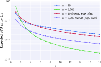
Figure 3: The leading entries of the expected SFS $\bolds{\xi}_{n}$ for a piecewise-exponential population size model inferred b Tennessen et al. tennessen:2012 . This demographic model, shown (up to scaling) in Figure 1, was fitted using the observed SFS from a sample of $1351$ (diploid) individuals of European ancestry tennessen:2012 . The blue plot is the expected SFS for $n=19$, which matches the sample size bound in Corollary 8 for identifying piecewise-exponential models with up to 5 pieces, while the green plot is the first 18 entries of the expected SFS for $n=2702$ ($1351$ diploids). The red and purple plots are the expected SFS for $n=19$ and $n=2702$, respectively, for a constant population size function.

On the other hand, our identifiability results show that perfect data (i.e., the exact expected SFS) from even a small sample size of $n=4K-1$ are sufficient to uniquely identify a piecewise-exponential model with $K$ pieces. This gap between theoretical identifiability and practical inference needs to be better addressed through robustness results that can account for the finite genome length, which limits the resolution to which the expected SFS of a random sample can be estimated. Our identifiability results apply in the limit that the genome length is infinite, which allows one to estimate the entries of the expected SFS exactly. On the other hand, a finite length genome does not permit exact estimation of the expected SFS, which can make it difficult in practice to resolve the details of ancient demographic events even if the sample size is large. This is because population size changes sufficiently far back in the past are likely to have only a marginal effect on the SFS since the individuals in the sample are highly likely to have found a common ancestor by such ancient times.

Our work suggests several interesting avenues for future research. An important problem is to understand the sensitivity of the SFS to perturbations in the demographic parameters. A related problem is quantifying the extent to which errors in estimating the expected SFS from a finite amount of data affect the parameter estimates in inferred demographic models.

It would also be interesting to consider the possibility of developing an algebraic algorithm for demographic inference that closely mimics the linear algebraic proof of Corollary 7 provided in Section 3. For example, using a sample of size $K+1$, one could consider inferring a piecewise-constant model with $K$ pieces, with one piece for each of the most recent $K-1$ generations and another piece for the population size further back in time. (Here, we are considering a restricted class of piecewise-constant population size functions with fixed change points, so the minimum sample size needed for distinguishing such models using the SFS is $K+1$ rather than $2K$.) Such an algebraic algorithm could provide a more principled way of inferring demographic parameters, compared to existing inference methods that rely on optimization procedures which lack theoretical guarantees for functions with multiple local optima.

In our work, we focused on the identifiability of demography from the expected SFS data. However, if one were to use the complete sequence data or other summary statistics such as the length distribution of shared haplotype tracts, it might be possible to uniquely identify the demography using even smaller sample sizes than that needed when using only the SFS. Indeed, several demographic inference methods have been developed to infer historical population size changes from such data using anywhere from a pair of genomic sequences li:2011 , harris:2013 , palamara:2012 to tens of such sequences sheehan:2013 , and it is important to theoretically characterize the power and limitations of both the data and the inference methods.

References

- (1) {bmisc}[pbm] \borganization1000 Genomes Project Consortium (\byear2010). \bhowpublishedA map of human genome variation from population-scale sequencing. Nature 467 1061–1073. \biddoi=10.1038/nature09534, issn=1476-4687, mid=UKMS34220, pii=nature09534, pmcid=3042601, pmid=20981092 \bptokimsref\endbibitem
- (2) {barticle}[author] \bauthor\bsnmBoyko, \bfnmAdam R.\binitsA. R., \bauthor\bsnmWilliamson, \bfnmScott H.\binitsS. H., \bauthor\bsnmIndap, \bfnmAmit R.\binitsA. R., \bauthor\bsnmDegenhardt, \bfnmJeremiah D.\binitsJ. D., \bauthor\bsnmHernandez, \bfnmRyan D.\binitsR. D., \bauthor\bsnmLohmueller, \bfnmKirk E.\binitsK. E., \bauthor\bsnmAdams, \bfnmMark D.\binitsM. D., \bauthor\bsnmSchmidt, \bfnmSteffen\binitsS., \bauthor\bsnmSninsky, \bfnmJohn J.\binitsJ. J., \bauthor\bsnmSunyaev, \bfnmShamil R.\binitsS. R. \betalet al. (\byear2008). \btitleAssessing the evolutionary impact of amino acid mutations in the human genome. \bjournalPLoS Genet. \bvolume4 \bpagese1000083. \bptokimsref\endbibitem
- (3) {barticle}[author] \bauthor\bsnmCampbell, \bfnmCatarina D.\binitsC. D., \bauthor\bsnmOgburn, \bfnmElizabeth L.\binitsE. L., \bauthor\bsnmLunetta, \bfnmKathryn L.\binitsK. L., \bauthor\bsnmLyon, \bfnmHelen N.\binitsH. N., \bauthor\bsnmFreedman, \bfnmMatthew L.\binitsM. L., \bauthor\bsnmGroop, \bfnmLeif C.\binitsL. C., \bauthor\bsnmAltshuler, \bfnmDavid\binitsD., \bauthor\bsnmArdlie, \bfnmKristin G.\binitsK. G. and \bauthor\bsnmHirschhorn, \bfnmJoel N.\binitsJ. N. (\byear2005). \btitleDemonstrating stratification in a European American population. \bjournalNat. Genet. \bvolume37 \bpages868–872. \bptokimsref\endbibitem
- (4) {barticle}[author] \bauthor\bsnmCoventry, \bfnmAlex\binitsA., \bauthor\bsnmBull-Otterson, \bfnmLara M.\binitsL. M., \bauthor\bsnmLiu, \bfnmXiaoming\binitsX., \bauthor\bsnmClark, \bfnmAndrew G.\binitsA. G., \bauthor\bsnmMaxwell, \bfnmTaylor J.\binitsT. J., \bauthor\bsnmCrosby, \bfnmJacy\binitsJ., \bauthor\bsnmHixson, \bfnmJames E.\binitsJ. E., \bauthor\bsnmRea, \bfnmThomas J.\binitsT. J., \bauthor\bsnmMuzny, \bfnmDonna M.\binitsD. M., \bauthor\bsnmLewis, \bfnmLora R.\binitsL. R. \betalet al. (\byear2010). \btitleDeep resequencing reveals excess rare recent variants consistent with explosive population growth. \bjournalNature Communications \bvolume1 \bpages131. \bptokimsref\endbibitem
- (5) {barticle}[pbm] \bauthor\bsnmExcoffier, \bfnmLaurent\binitsL., \bauthor\bsnmDupanloup, \bfnmIsabelle\binitsI., \bauthor\bsnmHuerta-Sánchez, \bfnmEmilia\binitsE., \bauthor\bsnmSousa, \bfnmVitor C.\binitsV. C. and \bauthor\bsnmFoll, \bfnmMatthieu\binitsM. (\byear2013). \btitleRobust demographic inference from genomic and SNP data. \bjournalPLoS Genet. \bvolume9 \bpagese1003905. \biddoi=10.1371/journal.pgen.1003905, issn=1553-7404, pii=PGENETICS-D-13-00576, pmcid=3812088, pmid=24204310 \bptokimsref\endbibitem
- (6) {barticle}[author] \bauthor\bsnmFu, \bfnmWenqing\binitsW., \bauthor\bsnmO’Connor, \bfnmTimothy D.\binitsT. D., \bauthor\bsnmJun, \bfnmGoo\binitsG., \bauthor\bsnmKang, \bfnmHyun Min\binitsH. M., \bauthor\bsnmAbecasis, \bfnmGoncalo\binitsG., \bauthor\bsnmLeal, \bfnmSuzanne M.\binitsS. M., \bauthor\bsnmGabriel, \bfnmStacey\binitsS., \bauthor\bsnmAltshuler, \bfnmDavid\binitsD., \bauthor\bsnmShendure, \bfnmJay\binitsJ., \bauthor\bsnmNickerson, \bfnmDeborah A.\binitsD. A. \betalet al. (\byear2012). \btitleAnalysis of 6515 exomes reveals the recent origin of most human protein-coding variants. \bjournalNature \bvolume493 \bpages216–220. \bptokimsref\endbibitem
- (7) {barticle}[pbm] \bauthor\bsnmFu, \bfnmY. X.\binitsY. X. (\byear1995). \btitleStatistical properties of segregating sites. \bjournalTheor. Popul. Biol. \bvolume48 \bpages172–197. \biddoi=10.1006/tpbi.1995.1025, issn=0040-5809, pii=S0040-5809(85)71025-8, pmid=7482370 \bptokimsref\endbibitem
- (8) {bbook}[author] \bauthor\bsnmGantmacher, \bfnmFeliks R.\binitsF. R. (\byear2000). \btitleThe Theory of Matrices, Vol. 2. \bpublisherChelsea, \blocationNew York. \bptokimsref\endbibitem
- (9) {barticle}[author] \bauthor\bsnmGazave, \bfnmElodie\binitsE., \bauthor\bsnmChang, \bfnmDiana\binitsD., \bauthor\bsnmClark, \bfnmAndrew G.\binitsA. G. and \bauthor\bsnmKeinan, \bfnmAlon\binitsA. (\byear2013). \btitlePopulation growth inflates the per-individual number of deleterious mutations and reduces their mean effect. \bjournalGenetics \bvolume195 \bpages969–978. \bptokimsref\endbibitem
- (10) {barticle}[author] \bauthor\bsnmGravel, \bfnmSimon\binitsS., \bauthor\bsnmHenn, \bfnmBrenna M.\binitsB. M., \bauthor\bsnmGutenkunst, \bfnmRyan N.\binitsR. N., \bauthor\bsnmIndap, \bfnmAmit R.\binitsA. R., \bauthor\bsnmMarth, \bfnmGabor T.\binitsG. T., \bauthor\bsnmClark, \bfnmAndrew G.\binitsA. G., \bauthor\bsnmYu, \bfnmFuli\binitsF., \bauthor\bsnmGibbs, \bfnmRichard A.\binitsR. A., \bauthor\bsnmBustamante, \bfnmCarlos D.\binitsC. D., \bauthor\bsnmAltshuler, \bfnmDavid L.\binitsD. L. \betalet al. (\byear2011). \btitleDemographic history and rare allele sharing among human populations. \bjournalProc. Natl. Acad. Sci. USA \bvolume108 \bpages11983–11988. \bptokimsref\endbibitem
- (11) {barticle}[author] \bauthor\bsnmGriffiths, \bfnmR. C.\binitsR. C. (\byear2003). \btitleThe frequency spectrum of a mutation, and its age, in a general diffusion model. \bjournalTheor. Popul. Biol. \bvolume64 \bpages241–251. \bptokimsref\endbibitem
- (12) {barticle}[mr] \bauthor\bsnmGriffiths, \bfnmR. C.\binitsR. C. and \bauthor\bsnmTavaré, \bfnmSimon\binitsS. (\byear1998). \btitleThe age of a mutation in a general coalescent tree. \bjournalComm. Statist. Stochastic Models \bvolume14 \bpages273–295. \biddoi=10.1080/15326349808807471, issn=0882-0287, mr=1617552 \bptokimsref\endbibitem
- (13) {barticle}[pbm] \bauthor\bsnmGutenkunst, \bfnmRyan N.\binitsR. N., \bauthor\bsnmHernandez, \bfnmRyan D.\binitsR. D., \bauthor\bsnmWilliamson, \bfnmScott H.\binitsS. H. and \bauthor\bsnmBustamante, \bfnmCarlos D.\binitsC. D. (\byear2009). \btitleInferring the joint demographic history of multiple populations from multidimensional SNP frequency data. \bjournalPLoS Genet. \bvolume5 \bpagese1000695. \biddoi=10.1371/journal.pgen.1000695, issn=1553-7404, pmcid=2760211, pmid=19851460 \bptokimsref\endbibitem
- (14) {barticle}[pbm] \bauthor\bsnmHarris, \bfnmKelley\binitsK. and \bauthor\bsnmNielsen, \bfnmRasmus\binitsR. (\byear2013). \btitleInferring demographic history from a spectrum of shared haplotype lengths. \bjournalPLoS Genet. \bvolume9 \bpagese1003521. \biddoi=10.1371/journal.pgen.1003521, issn=1553-7404, pii=PGENETICS-D-12-02556, pmcid=3675002, pmid=23754952 \bptokimsref\endbibitem
- (15) {barticle}[author] \bauthor\bsnmJameson, \bfnmG. J. O.\binitsG. J. O. (\byear2006). \btitleCounting zeros of generalised polynomials: Descartes’ rule of signs and Laguerre’s extensions. \bjournalThe Mathematical Gazette \bvolume90 \bpages223–234. \bptokimsref\endbibitem
- (16) {barticle}[author] \bauthor\bsnmKeinan, \bfnmAlon\binitsA. and \bauthor\bsnmClark, \bfnmAndrew G.\binitsA. G. (\byear2012). \btitleRecent explosive human population growth has resulted in an excess of rare genetic variants. \bjournalScience \bvolume336 \bpages740–743. \bptokimsref\endbibitem
- (17) {barticle}[pbm] \bauthor\bsnmKeinan, \bfnmAlon\binitsA., \bauthor\bsnmMullikin, \bfnmJames C.\binitsJ. C., \bauthor\bsnmPatterson, \bfnmNick\binitsN. and \bauthor\bsnmReich, \bfnmDavid\binitsD. (\byear2007). \btitleMeasurement of the human allele frequency spectrum demonstrates greater genetic drift in East asians than in europeans. \bjournalNat. Genet. \bvolume39 \bpages1251–1255. \biddoi=10.1038/ng2116, issn=1546-1718, mid=NIHMS434817, pii=ng2116, pmcid=3586588, pmid=17828266 \bptokimsref\endbibitem
- (18) {barticle}[author] \bauthor\bsnmKidd, \bfnmJeffrey M.\binitsJ. M., \bauthor\bsnmGravel, \bfnmSimon\binitsS., \bauthor\bsnmByrnes, \bfnmJake\binitsJ., \bauthor\bsnmMoreno-Estrada, \bfnmAndres\binitsA., \bauthor\bsnmMusharoff, \bfnmShaila\binitsS., \bauthor\bsnmBryc, \bfnmKatarzyna\binitsK., \bauthor\bsnmDegenhardt, \bfnmJeremiah D.\binitsJ. D., \bauthor\bsnmBrisbin, \bfnmAbra\binitsA., \bauthor\bsnmSheth, \bfnmVrunda\binitsV., \bauthor\bsnmChen, \bfnmRong\binitsR. \betalet al. (\byear2012). \btitlePopulation genetic inference from personal genome data: Impact of ancestry and admixture on human genomic variation. \bjournalAm. J. Hum. Genet. \bvolume91 \bpages660–671. \bptokimsref\endbibitem
- (19) {barticle}[author] \bauthor\bsnmKimura, \bfnmMotoo\binitsM. (\byear1955). \btitleSolution of a process of random genetic drift with a continuous model. \bjournalProc. Natl. Acad. Sci. USA \bvolume41 \bpages144–150. \bptokimsref\endbibitem
- (20) {barticle}[author] \bauthor\bsnmKimura, \bfnmMotoo\binitsM. (\byear1969). \btitleThe number of heterozygous nucleotide sites maintained in a finite population due to steady flux of mutations. \bjournalGenetics \bvolume61 \bpages893. \bptokimsref\endbibitem
- (21) {barticle}[mr] \bauthor\bsnmKingman, \bfnmJ. F. C.\binitsJ. F. C. (\byear1982). \btitleThe coalescent. \bjournalStochastic Process. Appl. \bvolume13 \bpages235–248. \biddoi=10.1016/0304-4149(82)90011-4, issn=0304-4149, mr=0671034 \bptokimsref\endbibitem
- (22) {barticle}[mr] \bauthor\bsnmKingman, \bfnmJ. F. C.\binitsJ. F. C. (\byear1982). \btitleOn the genealogy of large populations. \bjournalJ. Appl. Probab. \bvolume19A \bpages27–43. \bidissn=0170-9739, mr=0633178 \bptokimsref\endbibitem
- (23) {bincollection}[mr] \bauthor\bsnmKingman, \bfnmJ. F. C.\binitsJ. F. C. (\byear1982). \btitleExchangeability and the evolution of large populations. In \bbooktitleExchangeability in Probability and Statistics (Rome, 1981) (\beditor\bfnmG.\binitsG. \bsnmKoch and \beditor\bfnmF.\binitsF. \bsnmSpizzichino, eds.) \bpages97–112. \bpublisherNorth-Holland, \blocationAmsterdam. \bidmr=0675968 \bptokimsref\endbibitem
- (24) {barticle}[pbm] \bauthor\bsnmLi, \bfnmHeng\binitsH. and \bauthor\bsnmDurbin, \bfnmRichard\binitsR. (\byear2011). \btitleInference of human population history from individual whole-genome sequences. \bjournalNature \bvolume475 \bpages493–496. \biddoi=10.1038/nature10231, issn=1476-4687, mid=UKMS36009, pii=nature10231, pmcid=3154645, pmid=21753753 \bptokimsref\endbibitem
- (25) {barticle}[author] \bauthor\bsnmLohmueller, \bfnmKirk E.\binitsK. E., \bauthor\bsnmIndap, \bfnmAmit R.\binitsA. R., \bauthor\bsnmSchmidt, \bfnmSteffen\binitsS., \bauthor\bsnmBoyko, \bfnmAdam R.\binitsA. R., \bauthor\bsnmHernandez, \bfnmRyan D.\binitsR. D., \bauthor\bsnmHubisz, \bfnmMelissa J.\binitsM. J., \bauthor\bsnmSninsky, \bfnmJohn J.\binitsJ. J., \bauthor\bsnmWhite, \bfnmThomas J.\binitsT. J., \bauthor\bsnmSunyaev, \bfnmShamil R.\binitsS. R., \bauthor\bsnmNielsen, \bfnmRasmus\binitsR. \betalet al. (\byear2008). \btitleProportionally more deleterious genetic variation in European than in African populations. \bjournalNature \bvolume451 \bpages994–997. \bptokimsref\endbibitem
- (26) {barticle}[pbm] \bauthor\bsnmLukic, \bfnmSergio\binitsS. and \bauthor\bsnmHey, \bfnmJody\binitsJ. (\byear2012). \btitleDemographic inference using spectral methods on SNP data, with an analysis of the human out-of-Africa expansion. \bjournalGenetics \bvolume192 \bpages619–639. \biddoi=10.1534/genetics.112.141846, issn=1943-2631, pii=genetics.112.141846, pmcid=3454885, pmid=22865734 \bptokimsref\endbibitem
- (27) {barticle}[pbm] \bauthor\bsnmLukić, \bfnmSergio\binitsS., \bauthor\bsnmHey, \bfnmJody\binitsJ. and \bauthor\bsnmChen, \bfnmKevin\binitsK. (\byear2011). \btitleNon-equilibrium allele frequency spectra via spectral methods. \bjournalTheor. Popul. Biol. \bvolume79 \bpages203–219. \biddoi=10.1016/j.tpb.2011.02.003, issn=1096-0325, mid=NIHMS284088, pii=S0040-5809(11)00016-5, pmcid=3410934, pmid=21376069 \bptokimsref\endbibitem
- (28) {barticle}[pbm] \bauthor\bsnmMarchini, \bfnmJonathan\binitsJ., \bauthor\bsnmCardon, \bfnmLon R.\binitsL. R., \bauthor\bsnmPhillips, \bfnmMichael S.\binitsM. S. and \bauthor\bsnmDonnelly, \bfnmPeter\binitsP. (\byear2004). \btitleThe effects of human population structure on large genetic association studies. \bjournalNat. Genet. \bvolume36 \bpages512–517. \biddoi=10.1038/ng1337, issn=1061-4036, pii=ng1337, pmid=15052271 \bptokimsref\endbibitem
- (29) {barticle}[pbm] \bauthor\bsnmMarth, \bfnmGabor T.\binitsG. T., \bauthor\bsnmCzabarka, \bfnmEva\binitsE., \bauthor\bsnmMurvai, \bfnmJanos\binitsJ. and \bauthor\bsnmSherry, \bfnmStephen T.\binitsS. T. (\byear2004). \btitleThe allele frequency spectrum in genome-wide human variation data reveals signals of differential demographic history in three large world populations. \bjournalGenetics \bvolume166 \bpages351–372. \bidissn=0016-6731, pii=166/1/351, pmcid=1470693, pmid=15020430 \bptokimsref\endbibitem
- (30) {barticle}[pbm] \bauthor\bsnmMyers, \bfnmSimon\binitsS., \bauthor\bsnmFefferman, \bfnmCharles\binitsC. and \bauthor\bsnmPatterson, \bfnmNick\binitsN. (\byear2008). \btitleCan one learn history from the allelic spectrum? \bjournalTheor. Popul. Biol. \bvolume73 \bpages342–348. \biddoi=10.1016/j.tpb.2008.01.001, issn=1096-0325, pii=S0040-5809(08)00003-8, pmid=18321552 \bptokimsref\endbibitem
- (31) {barticle}[author] \bauthor\bsnmNelson, \bfnmMatthew R.\binitsM. R., \bauthor\bsnmWegmann, \bfnmDaniel\binitsD., \bauthor\bsnmEhm, \bfnmMargaret G.\binitsM. G., \bauthor\bsnmKessner, \bfnmDarren\binitsD., \bauthor\bsnmJean, \bfnmPamela St\binitsP. S., \bauthor\bsnmVerzilli, \bfnmClaudio\binitsC., \bauthor\bsnmShen, \bfnmJudong\binitsJ., \bauthor\bsnmTang, \bfnmZhengzheng\binitsZ., \bauthor\bsnmBacanu, \bfnmSilviu-Alin\binitsS.-A., \bauthor\bsnmFraser, \bfnmDana\binitsD. \betalet al. (\byear2012). \btitleAn abundance of rare functional variants in 202 drug target genes sequenced in 14,002 people. \bjournalScience \bvolume337 \bpages100–104. \bptokimsref\endbibitem
- (32) {barticle}[pbm] \bauthor\bsnmPalamara, \bfnmPier Francesco\binitsP. F., \bauthor\bsnmLencz, \bfnmTodd\binitsT., \bauthor\bsnmDarvasi, \bfnmAriel\binitsA. and \bauthor\bsnmPe’er, \bfnmItsik\binitsI. (\byear2012). \btitleLength distributions of identity by descent reveal fine-scale demographic history. \bjournalAm. J. Hum. Genet. \bvolume91 \bpages809–822. \biddoi=10.1016/j.ajhg.2012.08.030, issn=1537-6605, pii=S0002-9297(12)00472-7, pmcid=3487132, pmid=23103233 \bptokimsref \endbibitem
- (33) {barticle}[author] \bauthor\bsnmPasaniuc, \bfnmBogdan\binitsB., \bauthor\bsnmZaitlen, \bfnmNoah\binitsN., \bauthor\bsnmLettre, \bfnmGuillaume\binitsG., \bauthor\bsnmChen, \bfnmGary K.\binitsG. K., \bauthor\bsnmTandon, \bfnmArti\binitsA., \bauthor\bsnmKao, \bfnmWH Linda\binitsW. L., \bauthor\bsnmRuczinski, \bfnmIngo\binitsI., \bauthor\bsnmFornage, \bfnmMyriam\binitsM., \bauthor\bsnmSiscovick, \bfnmDavid S.\binitsD. S., \bauthor\bsnmZhu, \bfnmXiaofeng\binitsX. \betalet al. (\byear2011). \btitleEnhanced statistical tests for GWAS in admixed populations: assessment using African Americans from CARe and a Breast Cancer Consortium. \bjournalPLoS Genet. \bvolume7 \bpagese1001371. \bptokimsref\endbibitem
- (34) {bbook}[mr] \bauthor\bsnmPetkovšek, \bfnmMarko\binitsM., \bauthor\bsnmWilf, \bfnmHerbert S.\binitsH. S. and \bauthor\bsnmZeilberger, \bfnmDoron\binitsD. (\byear1996). \btitle. \bpublisherA K Peters, \blocationWellesley, MA. \bidmr=1379802 \bptokimsref\endbibitem
- (35) {barticle}[author] \bauthor\bsnmPolanski, \bfnmAndrzej\binitsA., \bauthor\bsnmBobrowski, \bfnmAdam\binitsA. and \bauthor\bsnmKimmel, \bfnmMarek\binitsM. (\byear2003). \btitleA note on distributions of times to coalescence, under time-dependent population size. \bjournalTheor. Popul. Biol. \bvolume63 \bpages33–40. \bptokimsref\endbibitem
- (36) {barticle}[author] \bauthor\bsnmPolanski, \bfnmAndrzej\binitsA. and \bauthor\bsnmKimmel, \bfnmMarek\binitsM. (\byear2003). \btitleNew explicit expressions for relative frequencies of single-nucleotide polymorphisms with application to statistical inference on population growth. \bjournalGenetics \bvolume165 \bpages427–436. \bptokimsref\endbibitem
- (37) {barticle}[pbm] \bauthor\bsnmPrice, \bfnmAlkes L.\binitsA. L., \bauthor\bsnmPatterson, \bfnmNick J.\binitsN. J., \bauthor\bsnmPlenge, \bfnmRobert M.\binitsR. M., \bauthor\bsnmWeinblatt, \bfnmMichael E.\binitsM. E., \bauthor\bsnmShadick, \bfnmNancy A.\binitsN. A. and \bauthor\bsnmReich, \bfnmDavid\binitsD. (\byear2006). \btitlePrincipal components analysis corrects for stratification in genome-wide association studies. \bjournalNat. Genet. \bvolume38 \bpages904–909. \biddoi=10.1038/ng1847, issn=1061-4036, pii=ng1847, pmid=16862161 \bptokimsref\endbibitem
- (38) {barticle}[pbm] \bauthor\bsnmReppell, \bfnmMark\binitsM., \bauthor\bsnmBoehnke, \bfnmMichael\binitsM. and \bauthor\bsnmZöllner, \bfnmSebastian\binitsS. (\byear2012). \btitleFTEC: A coalescent simulator for modeling faster than exponential growth. \bjournalBioinformatics \bvolume28 \bpages1282–1283. \biddoi=10.1093/bioinformatics/bts135, issn=1367-4811, pii=bts135, pmcid=3338023, pmid=22441586 \bptokimsref\endbibitem
- (39) {barticle}[pbm] \bauthor\bsnmReppell, \bfnmMark\binitsM., \bauthor\bsnmBoehnke, \bfnmMichael\binitsM. and \bauthor\bsnmZöllner, \bfnmSebastian\binitsS. (\byear2014). \btitleThe impact of accelerating faster than exponential population growth on genetic variation. \bjournalGenetics \bvolume196 \bpages819–828. \biddoi=10.1534/genetics.113.158675, issn=1943-2631, pii=genetics.113.158675, pmcid=3948808, pmid=24381333 \bptokimsref\endbibitem
- (40) {barticle}[pbm] \bauthor\bsnmSankararaman, \bfnmSriram\binitsS., \bauthor\bsnmPatterson, \bfnmNick\binitsN., \bauthor\bsnmLi, \bfnmHeng\binitsH., \bauthor\bsnmPääbo, \bfnmSvante\binitsS. and \bauthor\bsnmReich, \bfnmDavid\binitsD. (\byear2012). \btitleThe date of interbreeding between Neandertals and modern humans. \bjournalPLoS Genet. \bvolume8 \bpagese1002947. \biddoi=10.1371/journal.pgen.1002947, issn=1553-7404, pii=PGENETICS-D-11-02724, pmcid=3464203, pmid=23055938 \bptokimsref\endbibitem
- (41) {barticle}[pbm] \bauthor\bsnmSchaffner, \bfnmStephen F.\binitsS. F., \bauthor\bsnmFoo, \bfnmCatherine\binitsC., \bauthor\bsnmGabriel, \bfnmStacey\binitsS., \bauthor\bsnmReich, \bfnmDavid\binitsD., \bauthor\bsnmDaly, \bfnmMark J.\binitsM. J. and \bauthor\bsnmAltshuler, \bfnmDavid\binitsD. (\byear2005). \btitleCalibrating a coalescent simulation of human genome sequence variation. \bjournalGenome Res. \bvolume15 \bpages1576–1583. \biddoi=10.1101/gr.3709305, issn=1088-9051, pii=15/11/1576, pmcid=1310645, pmid=16251467 \bptokimsref\endbibitem
- (42) {barticle}[pbm] \bauthor\bsnmSheehan, \bfnmSara\binitsS., \bauthor\bsnmHarris, \bfnmKelley\binitsK. and \bauthor\bsnmSong, \bfnmYun S.\binitsY. S. (\byear2013). \btitleEstimating variable effective population sizes from multiple genomes: A sequentially Markov conditional sampling distribution approach. \bjournalGenetics \bvolume194 \bpages647–662. \biddoi=10.1534/genetics.112.149096, issn=1943-2631, pii=genetics.112.149096, pmcid=3697970, pmid=23608192 \bptokimsref\endbibitem
- (43) {barticle}[author] \bauthor\bsnmSkoglund, \bfnmPontus\binitsP. and \bauthor\bsnmJakobsson, \bfnmMattias\binitsM. (\byear2011). \btitleArchaic human ancestry in East Asia. \bjournalProc. Natl. Acad. Sci. USA \bvolume108 \bpages18301–18306. \bptokimsref\endbibitem
- (44) {barticle}[author] \bauthor\bsnmTennessen, \bfnmJacob A.\binitsJ. A., \bauthor\bsnmBigham, \bfnmAbigail W.\binitsA. W., \bauthor\bsnmO’Connor, \bfnmTimothy D.\binitsT. D., \bauthor\bsnmFu, \bfnmWenqing\binitsW., \bauthor\bsnmKenny, \bfnmEimear E.\binitsE. E., \bauthor\bsnmGravel, \bfnmSimon\binitsS., \bauthor\bsnmMcGee, \bfnmSean\binitsS., \bauthor\bsnmDo, \bfnmRon\binitsR., \bauthor\bsnmLiu, \bfnmXiaoming\binitsX., \bauthor\bsnmJun, \bfnmGoo\binitsG. \betalet al. (\byear2012). \btitleEvolution and functional impact of rare coding variation from deep sequencing of human exomes. \bjournalScience \bvolume337 \bpages64–69. \bptokimsref\endbibitem
- (45) {barticle}[author] \bauthor\bsnmWilliamson, \bfnmScott H.\binitsS. H., \bauthor\bsnmHernandez, \bfnmRyan\binitsR., \bauthor\bsnmFledel-Alon, \bfnmAdi\binitsA., \bauthor\bsnmZhu, \bfnmLan\binitsL., \bauthor\bsnmNielsen, \bfnmRasmus\binitsR. and \bauthor\bsnmBustamante, \bfnmCarlos D.\binitsC. D. (\byear2005). \btitleSimultaneous inference of selection and population growth from patterns of variation in the human genome. \bjournalProc. Natl. Acad. Sci. USA \bvolume102 \bpages7882–7887. \bptokimsref\endbibitem
- (46) {barticle}[pbm] \bauthor\bsnmŽivković, \bfnmDaniel\binitsD. and \bauthor\bsnmStephan, \bfnmWolfgang\binitsW. (\byear2011). \btitleAnalytical results on the neutral non-equilibrium allele frequency spectrum based on diffusion theory. \bjournalTheor. Popul. Biol. \bvolume79 \bpages184–191. \biddoi=10.1016/j.tpb.2011.03.003, issn=1096-0325, pii=S0040-5809(11)00019-0, pmid=21426909 \bptokimsref\endbibitem