Exact spectral function for hole-magnon coupling in the ferromagnetic CuO₃-like chain

Abstract

We present the exact spectral function for a single oxygen hole with spin opposite to ferromagnetic order within a one-dimensional CuO₃-like spin chain. We find that local Kondo-like exchange interaction generates five different states in the strong coupling regime. It stabilizes a spin polaron which is a bound state of a moving charge dressed by magnon excitations, with essentially the same dispersion as predicted by mean field theory. We then examine in detail the evolution of the spectral function for increasing strength of the hole-magnon interaction. We also demonstrate that the $s$ and $p$ symmetry of orbital states in the conduction band are essentially equivalent to each other and find that the simplified models do not suffice to reproduce subtle aspects of hole-magnon coupling in the charge-transfer model.
— Published in: Phys. Rev. B 88, 115132 (2013).

I Introduction

The theoretical analysis of transition metal oxides, including cuprates, manganites and iron pnictides, requires faithful description of strongly correlated electrons which localize due to Coulomb interactions in partly filled $3d$ orbitals.Imada et al. (1998) These interactions lead to Mott insulators in undoped compounds, with spin and orbital degrees of freedom which interact with charge defects arising under doping Zaanen and Oleś (1993) — then the magnetic order and transport properties change due to subtle interplay between charge and magnetic/orbital degrees of freedom. Good examples are high temperature superconductivity in cuprates,Dagotto (1994); Lee et al. (2006); Ogata and Fukuyama (2008) or colossal magnetoresistance in manganites.Dagotto et al. (2001); *Dag05; Weiße and Fehske (2004); Tokura (2006) In these systems, the interaction between charge carriers and localized spins is of crucial importance and drives the observed evolution of magnetic order and transport properties, captured in double exchange mechanism.de Gennes (1960); van den Brink and Khomskii (1999); Takenaka et al. (2002); Oleś and Feiner (2002); *Fei05 These changes may also depend on subtle quantum effects in systems with coupled spin-orbital-charge degrees of freedom.Oleś (2012)

A well known problem is the dynamics of one hole added to oxygen orbitals which interacts with $S=1/2$ spins at Cu ions in CuO₂ planes of high temperature superconductors. The spins form an antiferromagnetic (AF) order due to the superexchange interaction. A complete treatment of this problem involes a three-band model, Emery (1987); *Var87; *Ole87 with Cu $x^{2}-y^{2}$ orbitals occupied by one hole each and O $2p$ orbitals along the bonds. Instead, theoretical studies focus frequently on simplified treatments which do not include all quantum effects related to charge carries interacting with spin excitations in phases with magnetic order. For example, following the idea of Zhang and Rice,Zhang and Rice (1988) a simplified single-band model has been derived for CuO₂ planes from the charge-transfer model,Jefferson et al. (1992); *Fei96; *Rai96 and next used to study the evolution of magnetic order with increasing hole doping. However, such effective models do not accurately describe the electronic states in lightly doped materials. For instance, even low doping of less than 5% charge carriers is sufficient to change the magnetic order in vanadatesFujioka et al. (2008); *Hor11 or in manganites.Sakai et al. (2010); *Ole11

Electronic states change radically when electrons or holes propagate in a background with magnetic order. The well known example is a single hole which is classically confined in an antiferromagnet,Trugman (1988) but develops a quasiparticle propagating on the scale of superexchange by its coupling to quantum spin fluctuations.Martínez and Horsch (1991) In contrast, a conduction electron in the ferromagnetic (FM) background propagates as a free particle, as known in FM semiconductors such as EuO or EuS. Nolting (1979) Here the electron spin oriented in the opposite way to the FM background scatters on magnon excitations which leads to rather complex many-body problem,Nolting and Oleś (1980); *Nol81 and to changes of the electronic structure with increasing temperature.Wegner et al. (1998) It was pointed outNolting et al. (1996) that a repeated emission and reabsorption of a magnon by the conduction electron results in an effective attraction between magnon and electron. This gives rise to a polaron-like quasiparticle, the magnetic polaron. Another excitation is due to a direct magnon emission or absorption by the electron, thereby flipping its own spin, leading to scattering states. Modifications of electronic structure due to polarons were also discussed in manganites,Daghofer et al. (2004) cobaltates, Daghofer et al. (2006) and vanadates.Avella et al. (2013)

The purpose of this paper is to analyze the formation of polaron-like features and scattering states in a tight-binding model motivated by the physical properties known from cuprates. Due to strong local Coulomb repulsion $U$ at $x^{2}-y^{2}$ orbitals of Cu ions, the model including holes in these orbitals and in the surrounding oxygen orbitals, called also a three-band model, reduces to a spin-fermion model.Zaanen and Oleś (1988); Prelovšek (1988) The latter describes an oxygen hole coupled to the neighboring spins by a Kondo-like antiferromagnetic (AF) exchange interaction. This local AF coupling frustrates the AF superexchange in CuO₂ planes and is responsible for a rapid decay of AF order under increasing doping. The main difficulty in treating the dynamics of a doped hole are the AF quantum fluctuations of the spin background, which have to be treated in an approximate way.Dagotto (1994); Lee et al. (2006); Ogata and Fukuyama (2008)

Only very few many-body problems are exactly solvable. Exact solutions are typically limited to one-dimensional (1D) models or to a very special choice of interaction parameters. However, an exact solution (i) provides always important physical insights into the nature of quantum states involved, (ii) could serve to test approximate treatments, and (iii) may be used to draw useful conclusions for experimental studies. Recently, it was pointed out that a hole in a FM system with a single magnon excitation provides valuable insights into the spectral properties of a doped hole moving in a spin polarized system.Möller et al. (2012a); *Mir12b Here we introduce a CuO₃-like spin-chain model, as studied for YBa₂Cu₃O₇ high temperature superconductors. Recently, excited states were investigated in AF CuO₃ chainsSchlappa et al. (2011) in Sr₂CuO₃ and an interesting interplay due to spin-orbital entanglementOleś (2012) was pointed out.Wohlfeld et al. (2011) Here we analyze exactly the spectral properties in a FM chain. As we show below, they include the polaron-like and scattering states when the moving carrier interacts with magnons.

The paper is organized as follows. In Sec. II we introduce a 1D model for a CuO₃ spin chain. The spectral function of a single charge added to the oxygen orbital with the spin opposite to the FM order is obtained exactly using the Green’s function method in Sec. III.1. In Sec. III.2 we present an approximate perturbative solution for the same problem of a charge carrier coupled to the FM background in the strong coupling regime, while the mean field solution is given in Sec. III.3. The numerical results are presented in Sec. IV and the exact results are compared with the approximate ones. Summary and conclusions are given in Sec. V, while certain details of the derivation outlined in Sec. III.1 are presented in the Appendix.

II The model

We consider a 1D model presented in Fig. 1, with the same structure as a CuO₃ 1D chain in YBa₂Cu₃O₇, and assume that spins with a general value $S$ occupy the transition metal sites. In case of copper oxides, holes localize at Cu ions and $S=1/2$. Spins $\{\mathbf{S}_{i}\}$ are coupled here by FM Heisenberg exchange interactions as in the case of simpler 1D models considered before, Möller et al. (2012a); *Mir12b while holes in oxygen orbitals represent charge degrees of freedom which couple to spins by a local AF exchange, similar to a hole added to a CuO₂ plane.Zaanen and Oleś (1988) We label the oxygen orbitals as follows: (i) $a_{i\pm\xi}$ is located in between the magnetic sites, where $\xi$ is a vector pointing from the Cu site towards the $a$ site on its right, and (ii) $b_{i\pm\zeta}$ is located above and below the magnetic sites, where $\zeta$ is a vector pointing from the Cu site towards the $b$ site above it. Taking the charge-transfer model for a charged Cu²⁺O${}_{3}^{2-}$ chain as a reference (physical vacuum) state, these orbitals are filled with electrons and contain no hole.

The 1D model Hamiltonian,

$$\mathcal{H}=\mathcal{T}+\mathcal{H}_{\mathrm{S}}+\mathcal{H}_{\mathrm{K}},$$ (1)

includes the kinetic (hopping) part $\mathcal{T}$, the FM exchange between localized spins, $\mathcal{H}_{\mathrm{S}}$, as well as Kondo-like AF exchange interactions between a charge carrier (hole) in different orbitals and neighboring localized spins, $\mathcal{H}_{\mathrm{K}}$. The hopping couples the $a$ and $b$ orbitals, see Fig. 1. Depending on the orbital symmetry, only one of the local combinations of $b$ orbitals contributes to $\mathcal{T}$ and $\mathcal{H}_{\mathrm{S}}$, so it is convenient to introduce their symmetric ($+$, for $s$ orbitals) or antisymmetric ($-$, for $p$ orbitals) combinations, $b_{i}^{\pm}=(b_{i+\zeta}\pm b_{i-\zeta})/\sqrt{2}$.

The various terms in the Hamiltonian (1) are:

$$\mathcal{T} =-t\sum_{i\sigma}\left\{(a_{i+\xi,\sigma}^{{\dagger}}\pm a_{i-\xi,\sigma}^{{\dagger}})b_{i\sigma}^{\pm}+\text{H.c.}\right\},$$ (2a)

$$\mathcal{H}_{\mathrm{K}} =J_{0}\sum_{i}\left(\mathbf{s}_{i+\xi}^{a}+\mathbf{s}_{i-\xi}^{a}+\mathbf{s}_{i}^{b}\right)\cdot\mathbf{S}_{i},$$ (2b)

$$\mathcal{H}_{\mathrm{S}} =-J\sum_{i}(\mathbf{S}_{i}\cdot\mathbf{S}_{i+1}-S^{2}),$$ (2c)

where $\mathbf{S}_{i}$ is a spin operator for the magnetic ion at site $i$, $\mathbf{s}_{m}$ is a spin operator for the respective oxygen hole in orbital $m=a,b$, and $S$ is the magnitude of a single localized spin on the magnetic sublattice. All the energy constants are positive ($t>0$, $J_{0}>0$, $J>0$) and therefore $\mathcal{H}_{\mathrm{S}}$ provides FM coupling between the localized spins, while $\mathcal{H}_{\mathrm{K}}$ describes an AF Kondo-like coupling between localized spins and conduction electrons.Zaanen and Oleś (1988)

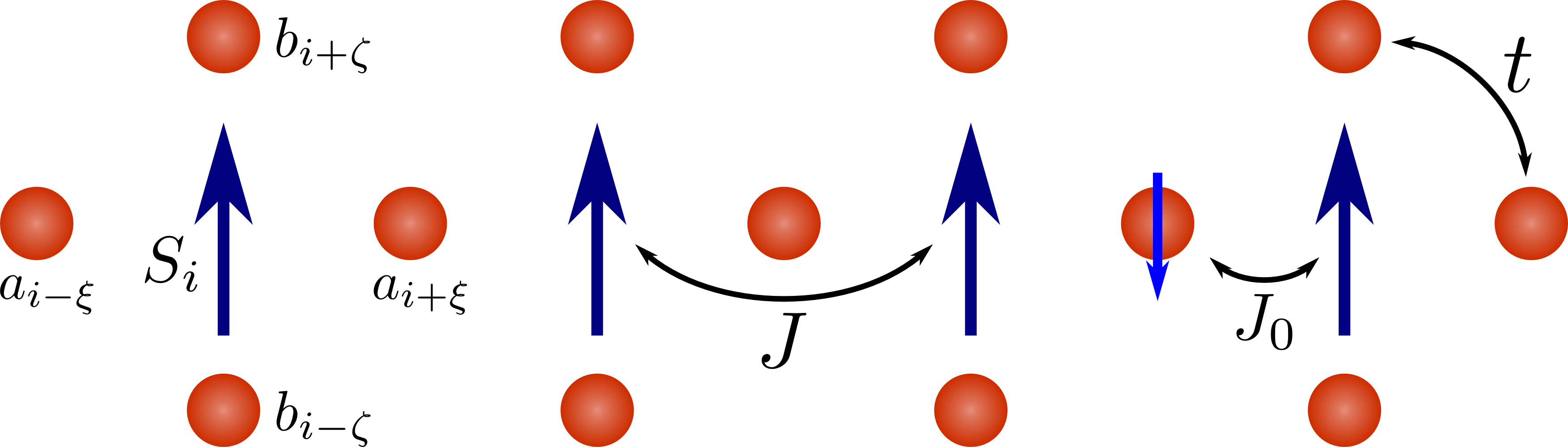
Figure 1: Graphic depiction of the CuO₃-like FM chain with localized spins indicated by arrows and oxygen ions indicated by filled circles. A hole added to an oxygen orbital (either $a_{i\pm\xi}$ or $b_{i\pm\zeta}$) interacts with the neighboring spin $S_{i}$ by the Kondo-like AF exchange $J_{0}$ while the localized spins interact by the FM exchange $J$. The hole hops between neighboring oxygen orbitals by the hopping $t$.

We study below the dynamics of a single hole injected into either of the conduction bands, which arise after $\mathcal{T}$ is diagonalized — one considers then two orbitals per unit cell and the Cu-Cu distance $a=1$. We will use the fermion representation for spin operators in the conduction band, $\mathbf{s}_{m}$. By transforming all the fermion operators to the reciprocal space by means of discrete Fourier transformation one arrives at the following representation of the Hamiltonian,

$$\mathcal{T} =\sum_{k\sigma}(\epsilon_{k}a_{k\sigma}^{{\dagger}}b_{k\sigma}+\text{H.c.}),$$ (3a)

$$\mathcal{H}_{\mathrm{K}} =J_{0}\sum_{kq}[2\cos(q/2)\,\mathbf{s}_{kq}^{a}+\mathbf{s}_{kq}^{b}]\cdot\mathbf{S}_{q},$$ (3b)

where $\epsilon_{k}$ follows from the Fourier fransformation and is given by

$$\epsilon_{k}=\begin{cases}-2t\cos(k/2)&\text{for $s$ symmetry}\\ +2it\sin(k/2)&\text{for $p$ symmetry}\end{cases}.$$ (4)

This leads to two bands $\varepsilon_{k}=\pm|\epsilon_{k}|$ for each value of $k\in[-\pi,\pi)$. The reciprocal-space spin operators are given by:

$$\mathbf{S}_{q} =\frac{1}{N}\sum_{i}e^{-iqR_{i}}\,\mathbf{S}_{i},$$ (5)

$$\mathbf{s}_{kq}^{\mu} =\begin{pmatrix}\tfrac{1}{2}(\mu_{k\uparrow}^{{\dagger}}\mu_{k+q\uparrow}-\mu_{k\downarrow}^{{\dagger}}\mu_{k+q\downarrow})\\ \mu_{k\uparrow}^{{\dagger}}\mu_{k+q\downarrow}\\ \mu_{k\downarrow}^{{\dagger}}\mu_{k+q\uparrow}\end{pmatrix}=\begin{pmatrix}\text{$s^{z}_{kq}$}\\ \text{$s^{+}_{kq}$}\\ \text{$s^{-}_{kq}$}\end{pmatrix},$$ (6)

where $\mu$ is an index labeling the states $\{a,b\}$. It should be emphasized that, strictly speaking, the operators $\mathbf{s}_{kq}^{\mu}$ are just a shorthand notation for the respective fermionic operators and should not be confused with regular spin operators. However, their effect in the spin subspace is similar.

As for $\mathcal{H}_{\mathrm{S}}$, its following eigenstates are easily identified:

$$\mathcal{H}_{\mathrm{S}}\lvert\text{FM}\rangle =0\lvert\text{FM}\rangle,$$ (7)

$$\mathcal{H}_{\mathrm{S}}S_{q}^{-}\lvert\text{FM}\rangle =\Omega_{q}S_{q}^{-}\lvert\text{FM}\rangle,$$ (8)

where $\lvert\text{FM}\rangle$ is the physical vacuum state, and $S_{q}^{-}\lvert\text{FM}\rangle$, defined by Eq. (5), is a magnetic excited state with one magnon (spin wave) created in the FM background and its energy dispersion

$$\Omega_{q}=4JS\sin^{2}(q/2).$$ (9)

Since the Hamiltonian under consideration conserves the total spin, these magnon states are the only attainable in the problem of a single hole with spin $s=1/2$ coupled to the FM spin background.

III Spin polaron and scattering states

III.1 Exact solution by Green’s functions

To obtain the hole spectral function we calculate first the Green’s function, defined by the expectation value of the resolvent,

$$\mathcal{G}(\omega)=[\omega-\mathcal{H}+i\eta]^{-1},$$ (10)

for the $\downarrow$-spin states of an added hole. Therefore, the Green’s function has a $2\times 2$ matrix structure:

$$\mathbb{G}_{\mu\nu}(k,\omega)=\langle\text{FM}\rvert\mu_{k\downarrow}\mathcal{G}(\omega)\nu_{k\downarrow}^{{\dagger}}\lvert\text{FM}\rangle,$$ (11)

where $\mu,\nu$ are again indices going over the states $\{a,b\}$. Following a method similar to the one described by Berciu and Sawatzky, Berciu and Sawatzky (2009) we divide the Hamiltonian, $\mathcal{H}_{0}=\mathcal{T}+\mathcal{H}_{\mathrm{S}}$, into the free part corresponding to $\mathcal{G}_{0}$, and the term $\mathcal{V}=\mathcal{H}_{\rm K}$ which couples the two subsystems by the AF interaction $\propto J_{0}$.

It is convenient to represent the Hamiltonian (3a) in terms of the following matrices:

$$\mathbb{T}(k) =\begin{pmatrix}0&\epsilon_{k}\\ \epsilon_{k}^{*}&0\end{pmatrix},$$ (12a)

$$\mathbb{V}(q) =\begin{pmatrix}\cos(q/2)&0\\ 0&\tfrac{1}{2}\end{pmatrix},$$ (12b)

while the form of $\mathbb{T}$ leads us to the matrix representation of $\mathcal{G}_{0}(\omega)$:

$$\mathbb{G}_{0}(k,\omega)=\begin{pmatrix}\omega+i\eta&-\epsilon_{k}\\ -\epsilon_{k}^{*}&\omega+i\eta\end{pmatrix}^{-1},$$ (13)

and in the case of one magnon state (8), the magnon energy $\Omega_{q}$ (9) is taken into account by substituting $\omega\to\omega-\Omega_{q}$. The inverse could also be calculated explicitly; however, it is not necessary for the present derivation.

We then proceed by utilizing the Dyson’s equation,

$$\mathcal{G}(\omega)=\mathcal{G}_{0}(\omega)+\mathcal{G}(\omega)\mathcal{V}\mathcal{G}_{0}(\omega),$$ (14)

which, after separating $\mathbb{G}(k,\omega)$, leads to the following matrix equation,

$$\mathbb{G}(k,\omega)=[\mathbb{I}+J_{0}\mathbb{F}(k,\omega)]\mathbb{G}_{0}(k,\omega)\mathbb{Q}_{G}(k,\omega),$$ (15)

where the various auxiliary matrices are given by:

$$\mathbb{F}(k,\omega) =\sum_{q}\mathbb{\tilde{F}}(k,q,\omega)\mathbb{V}(q),$$ (16)

$$\mathbb{\tilde{F}}_{\mu\nu}(k,q,\omega) =\langle\text{FM}\rvert\mu_{k\downarrow}\mathcal{G}(\omega)\nu_{k-q,\uparrow}^{{\dagger}}S_{q}^{-}\lvert\text{FM}\rangle.$$ (17)

Here $\mathbb{\tilde{F}}(k,q,\omega)$ is the anomalous Green’s function, calculated between different magnon states, resulting from the $S^{-}$ terms in $\mathcal{V}$, and

$$\mathbb{Q}_{G}(k,\omega) =\big{[}\mathbb{I}+J_{0}S\mathbb{V}_{0}\mathbb{G}_{0}(k,\omega)\big{]}^{-1},$$ (18)

$$\mathbb{V}_{0} =\sum_{q}\mathbb{V}(q)\delta_{q0}=\begin{pmatrix}1&0\\ 0&\frac{1}{2}\end{pmatrix},$$ (19)

where $\mathbb{Q}_{G}(k,\omega)$ is a transformation of $\mathbb{G}_{0}(k,\omega)$, performing a constant shift by $J_{0}S$. However, this cannot be written shortly as $\mathbb{G}_{0}(k,\omega+J_{0}S)$, because of the matrix $\mathbb{V}_{0}$ present in $\mathbb{Q}_{G}(k,\omega)$, which causes a different shift of ${J_{0}S}/{2}$ in the $G_{0}^{bb}(k,\omega)$ sector.

The next step is to eliminate $\mathbb{F}(k,\omega)$ from Eq. (15). In order to do this, one needs to express $\mathbb{\tilde{F}}(k,\omega)$ explicitly in terms of $\mathbb{G}(k,\omega)$ by applying the Dyson’s equation (14) once again and next solving for $\mathbb{F}(k,\omega)$. After inserting it back into Eq. (15) and solving for $\mathbb{G}(k,\omega)$, one arrives at the final result,

$$\mathbb{G}(k,\omega)=\mathbb{G}_{0}(k,\omega)\mathbb{Q}_{G}(k,\omega)\Big{[}\mathbb{I}-2J_{0}S\big{(}\mathbb{I}-\mathbb{M}^{-1}(k,\omega)\big{)}\mathbb{G}_{0}(k,\omega)\mathbb{Q}_{G}(k,\omega)\Big{]}^{-1},$$ (20)

where $\mathbb{M}$ is a complicated matrix expressed solely, in terms of various sums of $\mathbb{G}_{0}(k-q,\omega-\Omega_{q})$ over $q$. More details are presented in the Appendix. We note that this solution is almost identical to the one obtained by Berciu in Ref. Berciu and Sawatzky, 2009, only here we arrive at a more general solution for the transformation of $\mathbb{G}_{0}(k,\omega)$. Finally, having calculated the Green’s function, one finds the spectral function,

$$\mathbb{A}(k,\omega)=-\frac{1}{\pi}\Im{[\mathbb{G}(k,\omega)]},$$ (21)

which is closely related to the density of states as well as to the photoemission spectra, and can be directly measured in angle resolved photoemission spectroscopy experiments. The main physical problem is its structure and possible quasiparticle (QP) states.

The Green’s function $\mathbb{G}(k,\omega)$, as calculated from Eq. (20), is generally not diagonal. This is usually not a problem, since both diagonal components of the spectral function are measured at once in experiment, which corresponds to the trace of the corresponding matrix (21),

$$A(k,\omega)=\operatorname{Tr}\mathbb{A}(k,\omega),$$ (22)

a quantity invariant under the change of basis. Thus, we also present here the traced spectral function $A(k,\omega)$. In order to get more physical insight into the exact solution, we will now derive the approximate solutions of the problem, in two opposite parameter regimes, strong and weak hole-magnon coupling.

III.2 Perturbative solution at strong coupling

First approach is the perturbation expansion, with the problem treated in the eigenbasis of $\mathcal{V}$. This solution is valid in the strong coupling limit $J_{0}\gg t$ and $J_{0}\gg J$, since we treat $\mathcal{T}$ and $\mathcal{H}_{\mathrm{S}}$ as small perturbations to $\mathcal{H}_{\mathrm{K}}$.

Given the conjectured states of the form $\mu_{k\downarrow}^{{\dagger}}\lvert\text{FM}\rangle$ and $\sum_{q}e^{iq\rho}\nu_{k-q,\uparrow}^{{\dagger}}S_{q}^{-}\lvert\text{FM}\rangle$ (where $\rho=0,\pm\xi$ depends on the specific orbital) a straightforward calculation shows that the eigenstates of $\mathcal{V}$ are:

$$\lvert\bar{a}\rangle_{k} =\sqrt{\frac{4S}{4S+1}}\left[a_{k\downarrow}^{{\dagger}}-\frac{1}{2S}\sum_{q}\cos\left(\frac{q}{2}\right)a_{k-q,\uparrow}^{{\dagger}}S_{q}^{-}\right]\lvert\text{FM}\rangle,$$ (23a)

$$\lvert\bar{b}\rangle_{k} =\sqrt{\frac{2S}{2S+1}}\left[b_{k\downarrow}^{{\dagger}}-\frac{1}{2S}\sum_{q}b_{k-q,\uparrow}^{{\dagger}}S_{q}^{-}\right]\lvert\text{FM}\rangle,$$ (23b)

$$\lvert m\rangle_{k} =\frac{1}{\sqrt{S}}\sum_{q}\sin\left(\frac{q}{2}\right)a_{k-q,\uparrow}^{{\dagger}}S_{q}^{-}\lvert\text{FM}\rangle,$$ (23c)

$$\lvert b\rangle_{k} =\frac{1}{\sqrt{2S+1}}\left[b_{k\downarrow}^{{\dagger}}+\sum_{q}b_{k-q,\uparrow}^{{\dagger}}S_{q}^{-}\right]\lvert\text{FM}\rangle,$$ (23d)

$$\lvert a\rangle_{k} =\frac{1}{\sqrt{4S+1}}\left[a_{k\downarrow}^{{\dagger}}+2\sum_{q}\cos\left(\frac{q}{2}\right)a_{k-q,\uparrow}^{{\dagger}}S_{q}^{-}\right]\lvert\text{FM}\rangle.$$ (23e)

The first two states are bound polaronic states, and the last two ones are the respective excited states. The remaining state $\lvert m\rangle_{k}$ is a state dominated by magnons which dress an $\uparrow$-spin hole that propagates over $a$ orbitals. These definitions allow us to infer something about the approximate nature of different bands calculated from the Green’s function. Further, because $\mathcal{V}$ does not involve any three-site interaction terms but only self-renormalizing exchange interaction, there is no distinction between $s$ and $p$ orbitals, and therefore in both cases the states derived in perturbation theory (23) are the same. Using them, one can calculate the perturbation corrections to their energy coming from $\mathcal{H}_{\mathrm{S}}$ and $\mathcal{T}$. Owing to the specific orbital symmetries in the latter, in order to get a nontrivial contribution (i.e., dispersion) one needs to conduct the perturbation expansion at least up to the second order. The resulting energies for the states (23) are, respectively:

$$E_{\bar{a}} =-J_{0}\frac{(2S+1)}{2}+J\frac{2S}{4S+1}-\frac{\epsilon_{k}^{2}}{J_{0}}\frac{1}{(2S+1)}\left[\frac{(4S+1)}{S}+\frac{2S}{(4S+1)(3S+1)}\right]\,,$$ (24a)

$$E_{\bar{b}} =-J_{0}\frac{S+1}{2}+J\frac{2S}{2S+1}+\frac{\epsilon_{k}^{2}}{J_{0}}\frac{4S+1}{S(2S+1)}-\frac{\epsilon_{k-\pi}^{2}}{J_{0}}\frac{1}{3S(2S+1)}\,,$$ (24b)

$$E_{m} =J_{0}\frac{2S-1}{2}+J2S+\frac{\epsilon_{k-\pi}^{2}}{J_{0}}\frac{1}{2S+1}\left[\frac{1}{3S}-\frac{2S}{1-S}\right]\,,$$ (24c)

$$E_{b} =J_{0}\frac{S}{2}+J\frac{4S^{2}}{2S+1}+\frac{\epsilon_{k}^{2}}{J_{0}}\frac{2}{4S+1}\left[\frac{S}{(2S+1)(3S+1)}-\frac{2S+1}{S}\right]+\frac{\epsilon_{k-\pi}^{2}}{J_{0}}\frac{2S}{(2S+1)(1-S)}\,,$$ (24d)

$$E_{a} =J_{0}S+J\frac{8S^{2}}{4S+1}+\frac{\epsilon_{k}^{2}}{J_{0}}\frac{2(2S+1)}{S(4S+1)}\,.$$ (24e)

III.3 Mean field approximation

Another approximate approach to the problem is the mean field (MF) approximation for $\mathcal{V}$. In this case the principle is to neglect the quantum spin fluctuations in $\mathcal{H}_{\mathrm{K}}$, effectively setting $\mathbf{s}_{m}\cdot\mathbf{S}_{i}\approx s^{z}_{m}S_{i}^{z}$, where $\mathbf{s}_{m}$ stands for a spin in itinerant orbital, $a$ or $b$, in the neighborhood of site $i$. This assumption is valid provided the whole $\mathcal{H}_{\rm K}$ brings only a minor contribution to the overall energy, therefore implying $J_{0}\ll t$ and $J_{0}\ll J$. From Eq. (17) it follows that neglecting spin fluctuations implies $\tilde{\mathbb{F}}(k,q,\omega)=0$, and thus (15) reduces to the MF solution of the Green’s function,

$$\mathbb{G}_{MF}(k,\omega)=\mathbb{G}_{0}(k,\omega)\mathbb{Q}_{G}(k,\omega).$$ (25)

This equation depends only on $\mathbb{G}_{0}(k,\omega)$ and can be solved analytically, yielding the mean field energy dispersion,

$$E_{MF}^{\pm}(k)=-\frac{3J_{0}S}{4}\pm\sqrt{\left(\frac{J_{0}S}{4}\right)^{2}+\epsilon_{k}^{2}}.$$ (26)

This is also an exact solution of the model (1) with Ising interactions in $\mathcal{H}_{\rm K}$, and the deviation from it, reported in Sec. IV, is due to quantum spin fluctautions.

Furthermore, as already stated, Eq. (25) really corresponds to $\mathbb{G}_{0}(k,\omega)$ shifted by $J_{0}S$ in the case of $a$ band, and by $J_{0}S/2$ in the case of $b$ states. Therefore, we expect the MF solution (26) to resemble the free hole dispersion, shifted to the lower energy range by the appropriate value, and with an energy gap of $J_{0}S/2$ — indeed this is the case, as we show in a broad range of parameters in Sec. IV. We analyze there whether this prediction of the MF approximation holds beyond the regime of weak coupling $J_{0}\ll t$.

On the one hand, the two approximations described above are expected to coincide with the exact solution in their respective parameter ranges. Being among the most established approximate methods for quantum many-body systems, they serve as benchmarks of the method used here. On the other hand, comparing their predictions with the exact solution in the intermediate parameter range, i.e. $J_{0}\sim t$ and $J_{0}\sim J$, can give us a better understanding of how biased exactly those methods are. This is especially the case for the MF approach which is often employed as a first attempt at tackling a complicated problem.

IV Numerical results

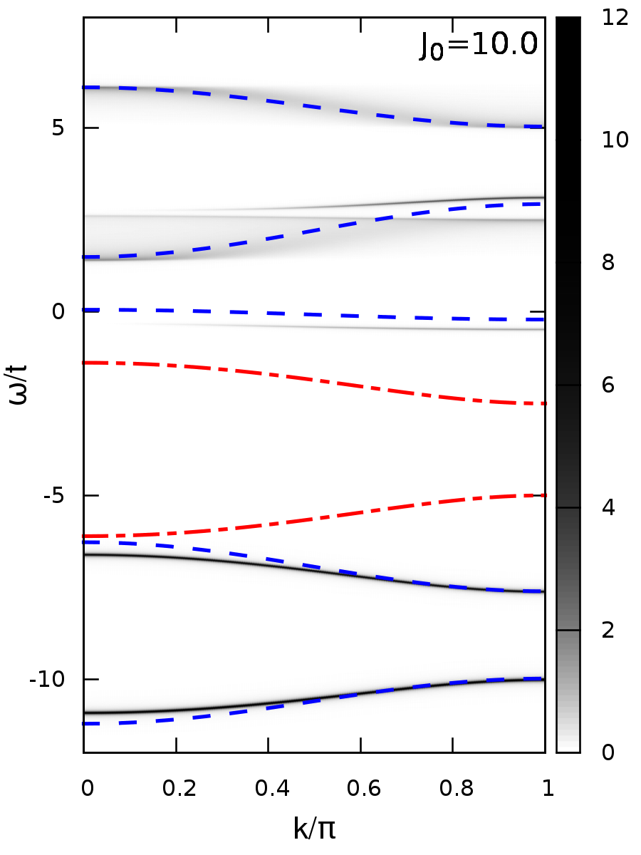
Figure 2: Spectral function $A(k,\omega)$ density map for $s$ orbital symmetry (shaded areas) compared with the analytic solutions (24) obtained in perturbation theory in the strong coupling regime, shown by dashed (blue) lines. The dash-dotted (red) lines represent the MF states (26). Parameters: $J_{0}=10t$, $J=0.05t$, $\eta=0.02t$, $S=1/2$.

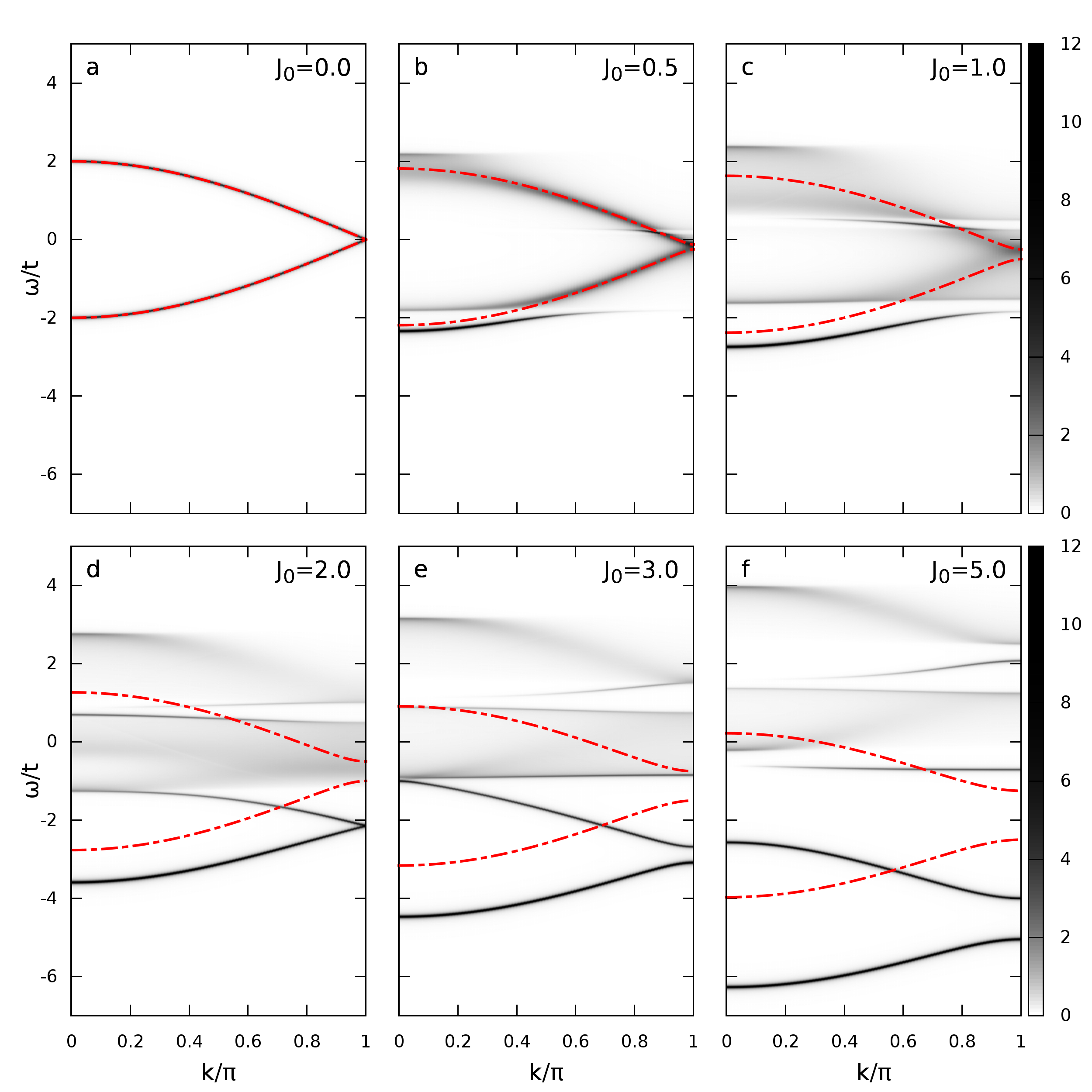
Figure 3: Spectral function $A(k,\omega)$ density maps obtained for a hole with $\downarrow$-spin added to a FM chain (1) for $s$ orbital symmetry. The dash-dotted (red) lines represent the MF states (26). Note the strongly nonlinear scale of the map, employed in order to bring out the low-amplitude incoherent spectra. Parameters: $J=0.05t$, $\eta=0.02t$, $S=1/2$.

The obtained result for the Green’s function Eq. (20) is exact, i.e., it follows from a rigorous derivation with no approximations employed, but unfortunately it does not allow one to calculate $\mathbb{G}(k,\omega)$ analytically. In particular, its central part, the matrix $\mathbb{M}(k,\omega)$, has to be obtained numerically. Below we present the numerical results obtained for the spectral function $A(k,\omega)$ using this exact scheme. In the numerical calculations we take $t=1$ as the energy unit and set $J=0.05t$, $\eta=0.02t$. We consider the case of $S=1/2$, where quantum spin fluctuations are the most important. We then explore the dependence of the spectra on the value of the coupling constant $J_{0}$ which controls the strength of the interaction between localized spins and a hole in $\mathcal{V}$.

Let us consider first the strong coupling limit of $J_{0}=10t$, see Fig. 2. In this regime one expects that the spectral function $A(k,\omega)$ consists of five features which correspond to the perturbative states (23), with distinct energies and rather weak dispersion. This analytic result is confirmed by a numerical solution, with the largest intensities obtained for the two states with the lowest energies. We remark that the states obtained in the perturbative regime have the same splitting of $J_{0}S/2$ at $k=\pi$ as in the MF theory, but they appear at a much lower energy due to formation of polaron states. This demonstrates the importance of quantum spin fluctuations in the binding energies of these polaronic states, which are neglected in the MF approximation. Quantum spin fluctuations enhance the binding energy roughly by $J_{0}/2$.

Consider next the systematic changes of the spectral functions with increasing exchange coupling $J_{0}$. Fig. 3 shows the spectral function density maps for the $s$ orbital symmetry for a wide range of $J_{0}$ values. For intermediate values of $J_{0}$ it consists of distinct QP states and shadded areas of scattering states. A nonlinear map scale has been applied in order to amplify the low-amplitude incoherent part of the spectrum, which in reality is negligibly small. The diversification of QP states caused by the interaction $\mathcal{V}$ can clearly be seen.

Starting from $J_{0}=0$ two branches are seen, corresponding to the free hole propagation of a $\downarrow$-spin hole and exactly replicate the MF solution. Since in this situation there is no interaction whatsoever, the added charge (hole) propagates without coupling to the magnetic background.

Next, for $J_{0}=0.5t$ the two branches are seen to have widened considerably and two new distinct features can be identified: (i) one directly below the lower band and corresponding to the first polaronic state $\lvert\bar{a}\rangle$, as shown by solutions obtained within perturbation theory and compared to the exact solution for large $J_{0}=10t$ (see Fig. 2), and (ii) the other one located slightly above $\omega=0$, and extending into the whole Brillouin zone for higher values of $J_{0}$. This latter feature fades away considerably and gradually develops into the upper bound of the lower incoherent region, corresponding to $\lvert b\rangle$ in the high coupling regime. At $J_{0}=t$ the original two branches have all but disappeared, and the lowest polaron state has almost fully developed.

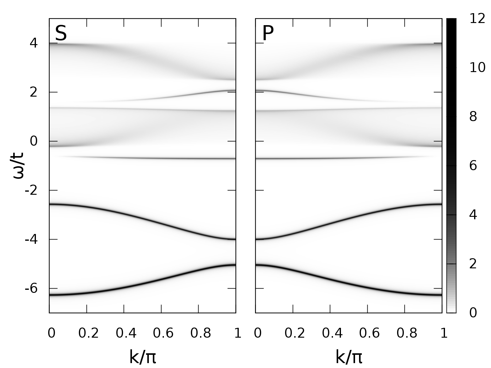
Figure 4: Comparison of the exact solutions for the spectral function $A(k,\omega)$ Eq. (22) obtained for $s$ symmetry orbitals in Fig. 1 (left) and for oxygen orbitals of $p$ symmetry (right). Parameters: $J_{0}=5t$, $J=0.05t$, $\eta=0.02t$ and $S=1/2$.

Increasing the interaction further to $J_{0}=2t$ we see that another state begins to emerge just slightly above the lowest polaronic state, starting from $k=\pi$. This state, corresponding to $\lvert\bar{b}\rangle$ in the strong coupling regime then slowly develops while lowering further below the incoherent continuum from which it emerged. Around this point the incoherent part of the spectrum develops a gap and divides into two distinct parts — the first of which has already been mentioned. The other one, situated at a higher energy, develops later into the $\lvert a\rangle$ state. Finally, at $J_{0}=5t$ yet another state can be seen situated close to $\omega=0$, seemingly with no dispersion. This state can be identified as $\lvert m\rangle$ and is purely magnonic, while the hole has the reversed $\uparrow$-spin.

While it is clear that MF gives good approximations for the weak coupling regime, a curious observation can be made about the strong coupling. Looking at the MF solutions plotted against the exact results for large values of $J_{0}$, one notices a surprising resemblance to the two lowest-lying states $\lvert\bar{a}\rangle$ and $\lvert\bar{b}\rangle$, save for some constant energy shift. This indicates that MF approximation can give relatively good qualitative results, predicting correct dispersion for polaronic states, but introduces a systematic error, as it neglects the binding energy coming from hole-magnon interaction. This explains the huge discrepancy between MF energies and the exact energies found for the polaron states.

It is also interesting to note that, while MF predicts the gap to develop monotonically, the real solution develops a gap shortly after the $\lvert\bar{a}\rangle$ state emerges from the incoherent region of the spectrum. This gap then closes again at around $J_{0}=2t$ and only after that does it reappear and start to widen monotonically. For more details on the evolution of the QP spectra with increasing parameter $J_{0}/t$, please refer to the Supplemental Material.sup

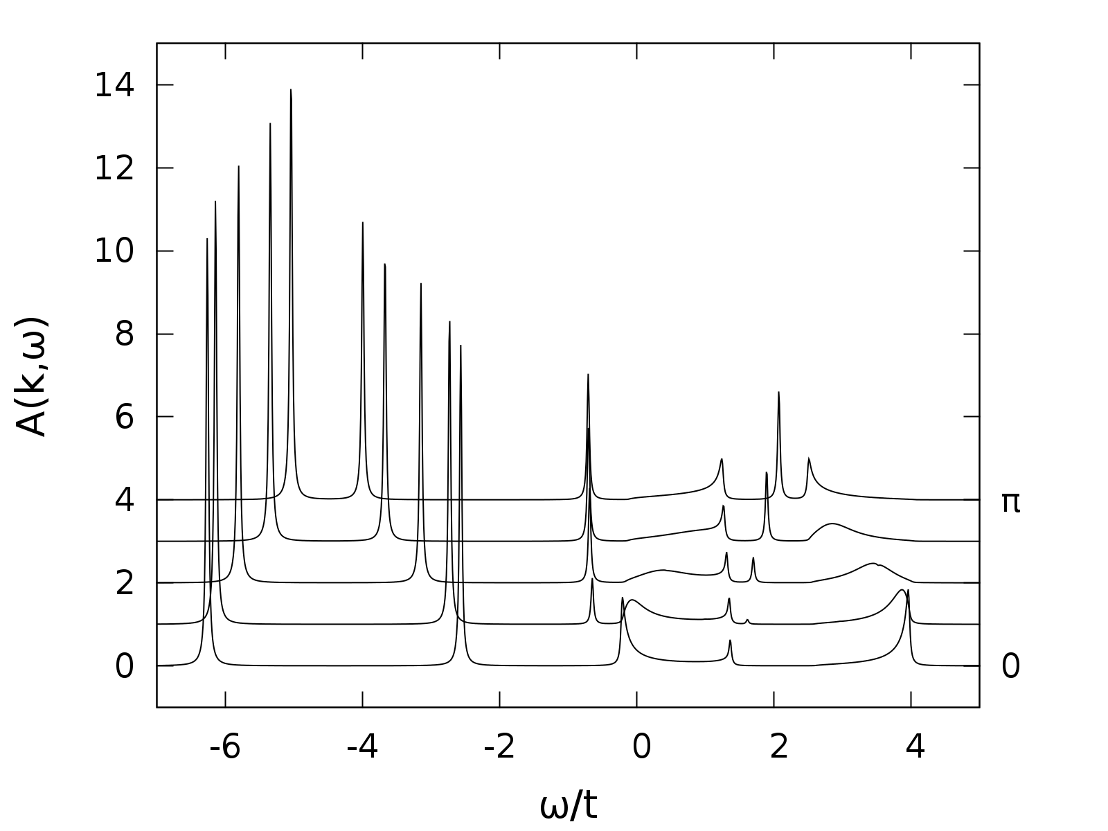
Figure 5: The spectral function $A(k,\omega)$ for selected values of $k=0,0.25\pi,0.5\pi,0.25\pi,\pi$, shown also in Fig. 3(f). Parameters: $J_{0}=5t$, $J=0.05t$, $\eta=0.02t$ and $S=1/2$.

Apart from calculations made for a wide range of $J_{0}$ values for $s$ symmetry, we have also done calculations for $p$ orbitals. However, because $\mathcal{V}$ in our model does not distinguish between the two, the only difference will come from their difference in dispersion. Taking into account that $\sin(k/2)=\cos[(\pi-k)/2]$, we expect the solution for $p$ orbitals to be a “mirror image” of the $s$-symmetry solutions with respect to momentum $k=\pi/2$. Fig. 4 clearly demonstrates that this indeed is the case.

While the spectral maps are very useful in presenting the entire spectra obtained for the present excat solution, they do not give one a good sense of detail. For this reason, in Fig. 5 we present an example of the spectra obtained for $J_{0}=5t$ for a few selected points $k\in[0,\pi]$ of the Brillouin zone. All the five spectral features corresponding to the states $\lvert\bar{a}\rangle_{k}$, $\lvert\bar{b}\rangle_{k}$, $\lvert m\rangle_{k}$, $\lvert b\rangle_{k}$ and $\lvert a\rangle_{k}$ can be well distinguished from one another. The two lowest states clearly have the largest spectral weights.

V Discussion and summary

We have used the method developed by Möller, Sawatzky and Berciu Möller et al. (2012a); *Mir12b to calculate the exact Green’s function and the spectral function for a simple model of a single hole moving in a CuO₃-like FM chain. Five distinct spectral features are identified — three of which arise from the hole propagating over the $a$ orbitals along the chain, and the other two follow from the hole within apical $b$ orbitals in a CuO₃-like chain. By introducing a realistic orbital structure for multi-band model, we addressed the problem of hole dynamics within $p$ orbitals in the charge-transfer model for a CuO₃ chain. We have then benchmarked this solution against the perturbation theory at strong coupling and mean field approximations. We have found that both of these approaches coincide quite well with the Green’s function solution in their respective regimes of applicability, i.e., mean field gives realistic predictions for weak interactions, while the perturbation theory reproduces all the states reasonably well in the strong coupling regime. The quantum states which develop beyond the mean field approximation will decrese their spectral weight with increasing value of spin $S$. In addition, the mean field approach seems to recreate the shapes of the polaronic bands at the strong coupling, but highly underrates the binding energy.

The perturbation solution allows us for identification of five distinct states: two well defined binding polaronic bands and one nearly dispersionless purely magnonic band, accompanied by two distinct excited polaronic states, coupled by a broad continuum. These latter excited states are much broader and have smaller spectral weights, even for very strong coupling $J_{0}\gg t$, which can be understood as following from the continuum of magnon excitations. Furthermore, the $\lvert b\rangle_{k},\lvert a\rangle_{k}$ and $\lvert m\rangle_{k}$ states which develop beyond the mean field approximation will decrease their spectral weight with increasing value of spin $S$ in the ferromagnetic chain. Indeed, the modifications of the spectra arising from quantum spin fluctuations are largest for $S=1/2$ and decrease with increasing $S$.

We also note that there is no essential difference between $s$ and $p$ orbital symmetries for the injected hole in the model Eq. (1), which is a result of taking into account only the exchange terms (second order two-site $p$-$d$-$p$ hopping). Therefore, such a simple model cannot properly describe a system with O-based conductance, reminiscent of doped cuprates. The simplest generalization of the present model is to include the three-site $p$-$d$-$p$ terms, Zaanen and Oleś (1988) which distinguish orbital symmetry. This is an interesting problem for future studies.

Appendix A Details of the exact solution Eq. (20)

Here we present the details of the calculation of the anomalous Green’s function $\tilde{\mathbb{F}}$. After applying the Dyson’s equation (14) to the Green’s function appearing in the definition given in Eq. (17), one obtains

$$\begin{split}\mathbb{\tilde{F}}_{\mu\nu}(k,q,\omega)&=\langle\text{FM}\rvert\mu_{k\downarrow}\mathcal{G}(\omega)\mathcal{V}\nu_{k-q,\uparrow}^{{\dagger}}S_{q}^{-}\lvert\text{FM}\rangle\\ &\times\mathbb{G}_{0}(k-q,\omega-\Omega_{q}),\end{split}$$ (27)

where the free-standing $\mathcal{G}_{0}(\omega)$ disappears due to the anomalous average.

Since the total spin of the system is conserved, only one spin-flip is allowed in the FM background interacting with the hole. Therefore, in the present case $\mathcal{V}$ can only leave the same defected state (which causes a renormalization of $\tilde{\mathbb{F}}(k,q,\omega)$) or may reproduce the initial FM state by means of a deexcitation of a magnon by a term $\propto S^{+}s^{-}$. This leads directly to the following equation:

$$\tilde{\mathbb{F}}(k,q,\omega) =\left[-\frac{J_{0}}{N}\sum_{p}\tilde{\mathbb{F}}(k,p,\omega)\mathbb{V}(q-p)+\frac{2J_{0}S}{N}\mathbb{G}(k,\omega)\mathbb{V}(q)\right]\mathbb{G}_{0}(k-q,\omega-\Omega_{q})\mathbb{Q}_{F}(k,q,\omega),$$ (28)

$$\mathbb{Q}_{F}(k,q,\omega) =\big{[}\mathbb{I}-J_{0}S\mathbb{V}_{0}\mathbb{G}_{0}(k-q,\omega-\Omega_{q})\big{]}^{-1}.$$ (29)

One has as well,

$$\mathbb{V}(q-p)=\begin{pmatrix}\cos\frac{q-p}{2}&0\\ 0&\frac{1}{2}\end{pmatrix}=\begin{pmatrix}\cos\frac{q}{2}&0\\ 0&\frac{1}{2}\end{pmatrix}\begin{pmatrix}\cos\frac{p}{2}&0\\ 0&\frac{1}{2}\end{pmatrix}+\begin{pmatrix}\sin\frac{q}{2}&0\\ 0&\frac{1}{2}\end{pmatrix}\begin{pmatrix}\sin\frac{p}{2}&0\\ 0&\frac{1}{2}\end{pmatrix}=\mathbb{V}(q)\mathbb{V}(p)+\bar{\mathbb{V}}(q)\bar{\mathbb{V}}(p),$$ (30)

and one finds,

$$\tilde{\mathbb{F}}(k,q,\omega)=\left[-\frac{J_{0}}{N}(\mathbb{F}(k,\omega)\mathbb{V}(q)+\bar{\mathbb{F}}(k,\omega)\bar{\mathbb{V}}(q))+\frac{2J_{0}S}{N}\mathbb{G}(k,\omega)\mathbb{V}(q)\right]\mathbb{G}_{0}(k-q,\omega-\Omega_{q})\mathbb{Q}_{F}(k,q,\omega),$$ (31)

where

$$\bar{\mathbb{F}}(k,\omega)=\sum_{p}\tilde{\mathbb{F}}(k,p,\omega)\bar{\mathbb{V}}(p).$$ (32)

$\mathbb{F}(k,\omega)$ used here is defined in Eq. (16). Multiplying now Eq. (31) either by $\mathbb{V}(q)$ or by $\bar{\mathbb{V}}(q)$ and summing over $q$, one can find explicit equations for $\mathbb{F}(k,\omega)$ and $\bar{\mathbb{F}}(k,\omega)$ in terms of $\mathbb{G}(k,\omega)$. Since $\bar{\mathbb{F}}(k,\omega)$ serves only as an auxiliary function, we will only present $\mathbb{F}(k,\omega)$ here:

$$\mathbb{F}(k,\omega)=2S\mathbb{G}(k,\omega)[\mathbb{I}-\mathbb{M}^{-1}(k,\omega)],$$ (33)

where we have already introduced the matrix $\mathbb{M}(k,\omega)$, defined as follows:

$$\begin{split}\mathbb{M}(k,\omega)&=\mathbb{I}+J_{0}\,\mathbb{G}_{cc}(k,\omega)-J_{0}^{2}\,\mathbb{G}_{cs}(k,\omega)\\ &\times[\mathbb{I}+J_{0}\mathbb{G}_{ss}(k,\omega)]^{-1}\mathbb{G}_{sc}(k,\omega),\end{split}$$ (34)

which is closely related to the self-energy. The auxiliary matrices introduced in Eq. (34) are:

$$\mathbb{G}_{cc} =\frac{1}{N}\sum_{q}\mathbb{V}(q)\mathbb{G}_{0}(k-q,\omega-\Omega_{q})\mathbb{V}(q),$$ (35a)

$$\mathbb{G}_{cs} =\frac{1}{N}\sum_{q}\mathbb{V}(q)\mathbb{G}_{0}(k-q,\omega-\Omega_{q})\bar{\mathbb{V}}(q),$$ (35b)

$$\mathbb{G}_{sc} =\frac{1}{N}\sum_{q}\bar{\mathbb{V}}(q)\mathbb{G}_{0}(k-q,\omega-\Omega_{q})\mathbb{V}(q),$$ (35c)

$$\mathbb{G}_{ss} =\frac{1}{N}\sum_{q}\bar{\mathbb{V}}(q)\mathbb{G}_{0}(k-q,\omega-\Omega_{q})\bar{\mathbb{V}}(q).$$ (35d)

After plugging the solution Eq. (33) into Eq. (15) and solving for $\mathbb{G}(k,\omega)$, one obtains the final result, Eq. (20) of Sec. III.1.

References

- Imada et al. (1998) M. Imada, A. Fujimori, and Y. Tokura, Rev. Mod. Phys. 70, 1039 (1998).
- Zaanen and Oleś (1993) J. Zaanen and A. M. Oleś, Phys. Rev. B 48, 7197 (1993).
- Dagotto (1994) E. Dagotto, Rev. Mod. Phys. 66, 763 (1994).
- Lee et al. (2006) P. A. Lee, N. Nagaosa, and X. G. Wen, Rev. Mod. Phys. 78, 17 (2006).
- Ogata and Fukuyama (2008) M. Ogata and H. Fukuyama, Rep. Prog. Phys. 71, 1 (2008).
- Dagotto et al. (2001) E. Dagotto, T. Hotta, and A. Moreo, Phys. Rep. 344, 1 (2001).
- Dagotto (2005) E. Dagotto, New J. Phys. 7, 67 (2005).
- Weiße and Fehske (2004) A. Weiße and H. Fehske, New J. Phys. 6, 158 (2004).
- Tokura (2006) Y. Tokura, Rep. Prog. Phys. 69, 797 (2006).
- de Gennes (1960) P. G. de Gennes, Phys. Rev. 118, 141 (1960).
- van den Brink and Khomskii (1999) J. van den Brink and D. Khomskii, Phys. Rev. Lett. 82, 1016 (1999).
- Takenaka et al. (2002) K. Takenaka, R. Shiozaki, and S. Sugai, Phys. Rev. B 65, 184436 (2002).
- Oleś and Feiner (2002) A. M. Oleś and L. F. Feiner, Phys. Rev. B 65, 052414 (2002).
- Feiner and Oleś (2005) L. F. Feiner and A. M. Oleś, Phys. Rev. B 71, 144422 (2005).
- Oleś (2012) A. M. Oleś, J. Phys.: Condens. Matter 24, 313201 (2012).
- Emery (1987) V. J. Emery, Phys. Rev. Lett. 58, 2794 (1987).
- Varma et al. (1987) C. M. Varma, S. S. Schmitt-Rink, and E. E. Abrahams, Solid State Commun. 62, 681 (1987).
- Oleś et al. (1987) A. M. Oleś, J. Zaanen, and P. Fulde, Physica B&C 148, 260 (1987).
- Zhang and Rice (1988) F. C. Zhang and T. M. Rice, Phys. Rev. B 37, 3759 (1988).
- Jefferson et al. (1992) J. H. Jefferson, H. Eskes, and L. F. Feiner, Phys. Rev. B 45, 7959 (1992).
- Feiner et al. (1996) L. F. Feiner, J. H. Jefferson, and R. Raimondi, Phys. Rev. B 53, 8751 (1996).
- Raimondi et al. (1996) R. Raimondi, J. H. Jefferson, and L. F. Feiner, Phys. Rev. B 53, 8774 (1996).
- Fujioka et al. (2008) J. Fujioka, S. Miyasaka, and Y. Tokura, Phys. Rev. B 77, 144402 (2008).
- Horsch and Oleś (2011) P. Horsch and A. M. Oleś, Phys. Rev. B 84, 064429 (2011).
- Sakai et al. (2010) H. Sakai, S. Ishiwata, D. Okuyama, A. Nakao, H. Nakao, Y. Murakami, Y. Taguchi, and Y. Tokura, Phys. Rev. B 82, 180409 (2010).
- Oleś and Khaliullin (2011) A. M. Oleś and G. Khaliullin, Phys. Rev. B 84, 214414 (2011).
- Trugman (1988) S. A. Trugman, Phys. Rev. B 37, 1597 (1988).
- Martínez and Horsch (1991) G. Martínez and P. Horsch, Phys. Rev. B 44, 317 (1991).
- Nolting (1979) W. Nolting, Phys. Status Solidi B 96, 11 (1979).
- Nolting and Oleś (1980) W. Nolting and A. M. Oleś, Phys. Rev. B 22, 6184 (1980).
- Nolting and Oleś (1981) W. Nolting and A. M. Oleś, Phys. Rev. B 23, 4122 (1981).
- Wegner et al. (1998) T. Wegner, M. Potthoff, and W. Nolting, Phys. Rev. B 57, 6211 (1998).
- Nolting et al. (1996) W. Nolting, S. M. Jaya, and S. Rex, Phys. Rev. B 54, 14455 (1996).
- Daghofer et al. (2004) M. Daghofer, A. M. Oleś, and W. von der Linden, Phys. Rev. B 70, 184430 (2004).
- Daghofer et al. (2006) M. Daghofer, P. Horsch, and G. Khaliullin, Phys. Rev. Lett. 96, 216404 (2006).
- Avella et al. (2013) A. Avella, P. Horsch, and A. M. Oleś, Phys. Rev. B 87, 045132 (2013).
- Zaanen and Oleś (1988) J. Zaanen and A. M. Oleś, Phys. Rev. B 37, 9423 (1988).
- Prelovšek (1988) P. Prelovšek, Phys. Lett. A 126, 287 (1988).
- Möller et al. (2012a) M. Möller, G. A. Sawatzky, and M. Berciu, Phys. Rev. Lett. 108, 216403 (2012a).
- Möller et al. (2012b) M. Möller, G. A. Sawatzky, and M. Berciu, Phys. Rev. B 86, 075128 (2012b).
- Schlappa et al. (2011) J. Schlappa et al., Nature 485, 82 (2011).
- Wohlfeld et al. (2011) K. Wohlfeld, M. Daghofer, S. Nishimoto, G. Khaliullin, and J. van den Brink, Phys. Rev. Lett. 107, 147201 (2011).
- Berciu and Sawatzky (2009) M. Berciu and G. A. Sawatzky, Phys. Rev. B 79, 195116 (2009).
- (44) See Supplemental Material at for an animated GIF, visualising the evolution of the spectra with increasing value of the Kondo-like exchange .