The Quark-Level Linear $\sigma$ Model

Abstract

This review of the quark-level linear $\sigma$ model (QLL$\sigma$M) is based upon the dynamical realization of the pseudoscalar and scalar mesons as a linear representation of $SU(2)\times SU(2)$ chiral symmetry, with the symmetry weakly broken by current quark masses. In its simplest $SU(2)$ incarnation, with two non-strange quark flavors and three colors, this nonperturbative theory, which can be selfconsistently bootstrapped in loop order, is shown to accurately reproduce a host of low-energy observables with only one parameter, namely the pion decay constant $f_{\pi}$. Extending the scheme to $SU(3)$ by including the strange quark, equally good results are obtained for many strong, electromagnetic, and weak processes just with two extra constants, viz. $f_{K}$ and $\langle\pi|H_{\mbox{\scriptsize weak}}|K\rangle$. Links are made with the vector-meson-dominance model, the BCS theory of superconductivity, and chiral-symmetry restoration at high temperature. Finally, these ideas are cautiously generalized to the electroweak sector, including the $W,Z$, and Higgs bosons, and also to CP violation.

1 Introduction

The magnitude of the strong interaction between the hadrons precludes the use of perturbation theory (PT) and this has been understood for a very long time. Only in the asymptotic high-energy regime, where the QCD coupling becomes logarithmically small, does it make any sense to use PT, and then only for the interactions involving gluons with their effective coupling. Thus it has been the goal of particle physicists to use nonperturbative schemes in order to tackle, with any semblance of reliability or conviction, the low-energy features of hadronic interactions. The sense of this approach is highlighted by the fact that the current quark masses are so much smaller than the constituent quark masses within the hadron, so that the extra mass is provided by the cloud of mesons and gluons which comprise the sum total. Foremost amongst these nonperturbative approaches has been the application of spontaneously broken chiral symmetry, accompanied by current algebra. For a good while the nonlinear realization of chiral symmetry at zero energy was used, together with an expansion in powers of momentum in order to get away from that particular limit. Unfortunately this has led to a plethora of expansion parameters and it blunts the use of the nonlinear theory predictions.

However it has also been found that the linear realization of chiral symmetry at the quark level is an alternative way of handling the low-energy properties of hadrons, without abandoning spontaneous breaking concepts introduced by Nambu [1]. In particular the Gell-Mann–Lévy model [2, 3], constrained by a vanishing of the renormalization constants of the mesons (which makes them composite states) is extremely predictive for a host of observed phenomena. Indeed it turns out that for pionic interactions essentially every low energy feature is determined completely just by one scale, the pion weak decay constant $f_{\pi}\simeq 92.2$ MeV. In the chiral limit, where the pion mass vanishes, all the other constants are totally fixed. Thus with just three colors, one can determine that

• the pion-quark coupling is $g=2\pi/\sqrt{3}$;

• the quartic pion-pion interaction is $\lambda=2g^{2}=8\pi^{2}/3$;

• the constituent nonstrange quark mass is $\hat{m}=f_{\pi}g\simeq 335$ MeV;

• the sigma meson partner to the pion has a mass $m_{\sigma}=2\hat{m}\simeq 670$ MeV.

It is even possible to extrapolate away from the chiral limit, by allowing for small current quark masses (which mar the chiral symmetry slightly) and thereby determine the deviations.

All this is explained in detail in Sects. 1, 2, and 3. There, as in succeeding sections, we compare the predictions of the quark-level linear $\sigma$ model (QLL$\sigma$M) with other methods, based on other premises. In Sec. 4 we revisit the compositeness condition ($Z=0$), and show how this can be used to set a demarcation scale between scalar and vector mesons. The importance of chiral cancellations is reviewed in Sec. 5, as it explains the vanishing of certain amplitudes, which might otherwise be quite large. This also affects the $\pi$-$N$ so-called sigma term associated with scattering lengths, treated in Sec. 6. Section 7 is devoted to the pion charge radius, which is again fully determined in terms of $f_{\pi}$ as $r_{\pi}=\hbar c\sqrt{3}/2\pi f_{\pi}\simeq 0.61$ fm, and can be contrasted with values obtained through the vector dominance model, incidentally explaining the value of the $\rho$-$\pi$-$\pi$ coupling constant as well. The breakdown of chiral symmetry at higher temperatures is considered next (Sec. 8), and this occurs at a critical temperature of $2f_{\pi}$; comparisons with the BCS (Bardeen, Cooper, Schrieffer [4]) and NJL (Nambu–Jona-Lasinio) [5]) models are described there, too.

In Sec. 9, we review the extension to $SU(3)$ by inclusion of the strange quark mass. Now the ratio $f_{K}/f_{\pi}$ fixes the constituent strange quark mass to be about 470 MeV, but its couplings to the quarks remain the same as the pion’s. Furthermore, the $\kappa$ analogue of the $\sigma$ meson is estimated to be about 797 MeV in mass. This is consonant with equal-mass splitting laws between scalar and pseudoscalar mesons, and in the process we review the mixing-angle parameters. Section 10 covers e.m. decay rates, as they constitute clean tests of all that has gone before and generally fit the data very well, including the isoscalar scalar $f_{0}(500)$ [6] meson. The other light scalar isoscalar $f_{0}(980)$, as well as its isovector partner $a_{0}(980)$, are dealt with in more detail in Sec. 11, in particular concerning their strong decays. Sections 12 and 13 are devoted to weak decays, which are governed by one new scale: the $K,\bar{K}$ matrix element of the weak Hamiltonian $H_{w}$, or equivalently the transition element $\langle\pi|H_{w}|K\rangle$. Ramifications of these ideas to other weak decays are also treated. The e.m. form factors of mesons, their role in certain weak decays, as well as the estimation of meson polarizabilities form the subject of Sec. 14. In Sec. 15 we establish a link between the critical temperature, mentioned in Sec. 8, and the BCS theory of superconductivity with its characteristic energy gap.

Section 16 makes an analogy between the QLL$\sigma$M and the standard electroweak model. In that picture the Higgs boson is regarded largely as a top-antitop scalar bound state with a mass of about 315 GeV, set by a weak decay constant of $f_{w}\simeq 246$ GeV. This picture is consonant with a weak KSRF (Kawarabayashi, Suzuki, Riazuddin, Fayyazuddin) [7, 8] relation and the observed masses of the weak vector bosons plus the weak mixing angle. Possible implications of recently observed [9, 10] Higgs-like signals at the large hadron collider (LHC) of CERN are discussed as well. We conclude this review in Sec. 17 by an analysis of CP violation, as supposed to arise from a nonstandard $WW\gamma$ vertex.

2 $\boldsymbol{SU(2)}$ QLL$\boldsymbol{\sigma}$M

First we state the $SU(2)$ quark-level linear $\sigma$ model (QLL$\sigma$M) Lagrangian density, with interacting part

$${\mathcal{L}}^{\mbox{\scriptsize L$\sigma$M}}_{\mbox{\scriptsize int}}\;=\;g\bar{\psi}(\sigma+i\gamma_{5}\vec{\tau}\cdot\vec{\pi})\psi+g^{\prime}\sigma(\sigma^{2}+\vec{\pi}^{2})-\frac{\lambda}{4}(\sigma^{2}+\vec{\pi}^{2})^{2}\;,$$ (1)

with the chiral-limiting (CL) pion-quark and meson-meson couplings

$$g\;=\;\frac{m_{q}}{f_{\pi}}\;\;\;,\;\;\;g^{\prime}\;=\;\frac{m^{2}_{\sigma}}{2f_{\pi}}=\lambda f_{\pi}\;.$$ (2)

This QLL$\sigma$M is in the spirit of the original Gell-Mann–Lévy L$\sigma$M [2, 3], but for quarks [11, 12] rather than for nucleon fermions, and also with Nambu–Goldstone [1, 13, 14] pseudoscalar pions, having vanishing mass in the chiral limit, i.e., $m_{\pi}^{\mbox{\scriptsize CL}}=0$. Note, however, that the nonstrange pion and sigma mesons in Eq. (1) are quantum fields which both vanish in the CL. Such a vanishing does not occur in [2, 3] for spin-$1/2$ nucleons, in contrast with the present QLL$\sigma$M scheme. Furthermore, in the chiral limit the nonstrange constituent quark mass $\hat{m}_{\mbox{\scriptsize con}}=(m_{u}+m_{d})/2$ is half the mass of the $\sigma$ meson, i.e.,

$$m_{\sigma}^{\mbox{\scriptsize CL}}\;=\;2\hat{m}_{\mbox{\scriptsize con}}^{\mbox{\scriptsize CL}}\;,$$ (3)

which is valid for both the QLL$\sigma$M of Eq. (1) and the nonlinear NJL [5] model. The Goldberger–Treiman relation (GTR) [15] for the QLL$\sigma$M reads $\hat{m}_{\mbox{\scriptsize con}}=f_{\pi}g$, which should be compared with the GTR for nucleons, viz. $g_{A}m_{N}=f_{\pi}g_{\pi NN}$, but now at the quark level, with $g_{A}$=1 for constituent quarks [16].

Next we follow [17, 18], and compute the pseudoscalar pion mass, which vanishes in the CL, via the selfenergy graphs of Figs. 2 and 1. [h]              
Pion-selfenergy quark-loop graphs. Left: bubble; right: $\sigma$ tadpole. The quark loops (QL) of Fig. 2 give a pion mass squared

$$m^{2}_{\pi,\mbox{\scriptsize QL}}\;=\;-i8N_{c}g^{2}\left(1-\frac{2g^{\prime}f_{\pi}}{m^{2}_{\sigma}}\right)\int\frac{\mathchar 22\relax\mkern-12.0mud\;\!^{4}\>\!\!p}{p^{2}-m^{2}_{q}}\;=\;0\;,$$ (4)

with $\mathchar 22\relax\mkern-12.0mud^{\,4}\>\!\!p\equiv d^{4}\>\!\!p/(2\pi)^{4}$. Now, $m^{2}_{\pi,\mbox{\scriptsize QL}}$ vanishes identically in the CL, since then $g^{\prime}=m^{2}_{\sigma}/2f_{\pi}$. As for the meson-loop (ML) graphs in Fig. 1,

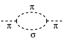
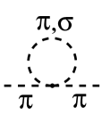
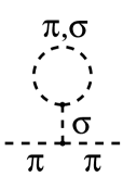
Figure 1: Pion-selfenergy meson-loop graphs. Left: bubble; middle: “snail”; right: tadpole.

we first invoke the partial-fraction identity

$$\frac{g^{\prime 2}}{(p^{2}-m^{2}_{\sigma})(p^{2}-m^{2}_{\pi})}\;=\;\frac{\lambda}{2}\left[\frac{1}{p^{2}-m^{2}_{\sigma}}-\frac{1}{p^{2}-m^{2}_{\pi}}\right]\;,$$ (5)

using $g^{\prime 2}=\lambda(m^{2}_{\sigma}-m^{2}_{\pi})/2$. Then, the contributions from the diagrams in Fig. 1 become

$$m^{2}_{\pi,\mbox{\scriptsize ML}}\;=\;i(-2\lambda+5\lambda-3\lambda)\int\frac{\mathchar 22\relax\mkern-12.0mud\;\!^{4}\>\!\!p}{p^{2}-m^{2}_{\pi}}\;+\;i(2\lambda+\lambda-3\lambda)\int\frac{\mathchar 22\relax\mkern-12.0mud\;\!^{4}\>\!\!p}{p^{2}-m^{2}_{\sigma}}\;=\;0\;.$$ (6)

Note that the coefficients of the quadratically divergent graphs in Fig. 1 vanish identically. Combining Eqs. (4) and (6) generates the vanishing Nambu-Goldstone pion mass in the CL

$$m^{2}_{\pi}\;=\;0\,|_{\mbox{\scriptsize quark loops}}\;+\;0\,|_{\mbox{\scriptsize$\pi$ loops}}\;+\;0\,|_{\mbox{\scriptsize$\sigma$ loops}}\;=\;0\;.$$ (7)

Such is the subtle beauty of chiral symmetry!

Now we determine the $\pi^{0}$ decay constant $f_{\pi}$. The latest data in the Particle Data Group (PDG) [6] tables give

$$f_{\pi}\;=\;(92.21\pm 0.15)\;\mbox{MeV}\;.$$ (8)

Also, the pion-quark coupling is [19, 20]

$$g_{\pi qq}\;=\;\frac{2\pi}{\sqrt{N_{c}}}\;\simeq\;3.6276\;,$$ (9)

a value to be reconfirmed shortly, for $N_{c}=3$ colors. Thus, the nonstrange constituent quark mass found via the GTR becomes

$$\hat{m}_{\mbox{\scriptsize con}}\;=\;f_{\pi}g_{\pi qq}\;=\;(92.21\>\mbox{MeV})\,\frac{2\pi}{\sqrt{3}}\;\simeq\;334.5\;\mbox{MeV}\;.$$ (10)

This value is slightly less than a quick estimate resulting from combining the proton mass with its magnetic moment, i.e., for $\hat{m}_{\mbox{\scriptsize con}}=(m_{u}+m_{d})_{\mbox{\scriptsize con}}/2$,

$$\hat{m}_{\mbox{\scriptsize con}}\;\simeq\;\frac{m_{p}}{\mu_{p}}\;\simeq\;\frac{938.27\>\mbox{MeV}}{2.7928}\;\simeq\;336.0\;\mbox{MeV}\;.$$ (11)

A more accurate computation from the proton magnetic moment, which takes into account a 4 MeV mass difference between the down and the up quark, yields the prediction [21]

$$\hat{m}_{\mbox{\scriptsize con}}\;\simeq\;337.5\;\mbox{MeV}\;,$$ (12)

which is just a little bit higher than in Eqs. (10,11).

Finally, we work in the CL to generate $f_{\pi}^{\mbox{\scriptsize CL}}$ via a once-subtracted dispersion relation [22, 23] (involving no arbitrary parameters as in chiral perturbation theory):

$$f_{\pi}-f_{\pi}^{\mbox{\scriptsize CL}}\;=\;\frac{m^{2}_{\pi}}{\pi}\int_{0}^{\infty}\frac{\Im\mbox{m}\,f_{\pi}(q^{2})\,dq^{2}}{q^{2}(q^{2}-m^{2}_{\pi})}\;=\;\frac{m^{2}_{\pi}}{8\pi^{2}f_{\pi}}\;.$$ (13)

With $f_{\pi}=92.21$ MeV and an average pion mass $m_{\pi}\simeq 137$ MeV, we thus find

$$1-\frac{f_{\pi}^{\mbox{\scriptsize CL}}}{f_{\pi}}\;=\;\frac{m^{2}_{\pi}}{8\pi^{2}f_{\pi}^{2}}\;\simeq\;2.8\%\;,$$ (14)

which in turn predicts

$$f_{\pi}^{\mbox{\scriptsize CL}}\;=\;f_{\pi}(1-0.028)\;\simeq\;89.63\;\mbox{MeV}\;.$$ (15)

Then, via the GTR, we get

$$\hat{m}_{\mbox{\scriptsize con}}^{\mbox{\scriptsize CL}}\;=\;f_{\pi}^{\mbox{\scriptsize CL}}g_{\pi qq}\;\simeq\;(89.63\;\mbox{MeV})\,\frac{2\pi}{\sqrt{3}}\;\simeq\;325.1\;\mbox{MeV}\;.$$ (16)

3 Dynamically generating the $\boldsymbol{SU(2)}$ QLL$\boldsymbol{\sigma}$M

Following [17, 18], we first compute the nonstrange quark loop in Fig. 3, [h]          
Pion nonstrange quark loop for the LDGE in Eq. (17). leading to the log-divergent gap equation (LDGE)

$$1\;=\;-i4N_{c}g^{2}\int\frac{\mathchar 22\relax\mkern-12.0mud\;\!^{4}\>\!\!p}{(p^{2}-m^{2}_{q})^{2}}\;,$$ (17)

due to the quark-loop integral for the neutral pion decay constant combined with the quark-level GTR (10). This LDGE also holds for the nonlinear NJL scheme in [5], and leads to many low-energy theorems [24]. Furthermore, the quark tadpole graph of Fig. 17 [h]
Quark-selfenergy tadpole graph. generates a counter-term mass gap

$$m_{q}\;=\;-\frac{8iN_{c}g^{2}}{m^{2}_{\sigma}}\int\frac{\mathchar 22\relax\mkern-12.0mud\;\!^{4}\>\!\!p}{p^{2}-m_{q}^{2}}m_{q}\;.$$ (18)

Then, canceling out the $m_{q}$ scale gives

$$m^{2}_{\sigma}\;=\;-8iN_{c}g^{2}\int\frac{\mathchar 22\relax\mkern-12.0mud\;\!^{4}\>\!\!p}{p^{2}-m_{q}^{2}}\;.$$ (19)

Lastly, the $\sigma$ bubble plus $\sigma$ tadpole graphs of Fig. 19 in the CL generate the counter-term relation [h]              
Sigma-meson selfenergy graphs. Left: quark bubble; right: $\sigma$ tadpole.

$$m^{2}_{\sigma,\mbox{\scriptsize CL}}\;=\;16iN_{c}g^{2}\!\int\,\mathchar 22\relax\mkern-12.0mud\;\!^{4}\>\!\!p\left[\frac{m_{q}^{2}}{(p^{2}-m_{q}^{2})^{2}}-\frac{1}{p^{2}-m_{q}^{2}}\right]_{\mbox{\scriptsize CL}}\;.$$ (20)

Substituting Eqs. (17,19) into Eq. (20) leads to the CL relation

$$m^{2}_{\sigma,\mbox{\scriptsize CL}}\;=\;-4m^{2}_{q,\mbox{\scriptsize CL}}+2m^{2}_{\sigma,\mbox{\scriptsize CL}}\;\;\;\Rightarrow\;\;\;m_{\sigma,\mbox{\scriptsize CL}}=2m_{q}^{\mbox{\scriptsize CL}}\;,$$ (21)

but now for the QLL$\sigma$M rather than for the nonlinear NJL model. Note that Eq. (21), together with Eq. (16), predicts $m_{\sigma}^{\mbox{\scriptsize CL}}\simeq 650.3$ MeV.

Moreover, the integral difference in Eq. (20) leads to the dimensional-regularization lemma (DRL) [17], via a Wick rotation:

$$\int\mathchar 22\relax\mkern-12.0mud\;\!^{4}\>\!\!p\left[\frac{m_{q}^{2}}{(p^{2}-m_{q}^{2})^{2}}-\frac{1}{p^{2}-m_{q}^{2}}\right]\;=\;-\frac{im^{2}_{q}}{16\pi^{2}}\;.$$ (22)

This result follows in many regularization schemes (dimensional, analytic, $\zeta$-function, Pauli-Villars) and also in a scheme-independent manner [25, 26]. Then, substituting Eq. (22) back into Eq. (20) leads to

$$m_{\sigma}^{\mbox{\scriptsize CL}}\;=\;\frac{\sqrt{N_{c}}}{\pi}\,g\,m_{q}^{\mbox{\scriptsize CL}}\;,$$ (23)

which predicts, also using Eq. (21) and $N_{c}=3$, the crucial coupling

$$g\;=\;g_{\pi qq}\;=\;\frac{2\pi}{\sqrt{N_{c}}}\;\simeq\;3.6276\;.$$ (24)

In fact, the latter result also holds [19, 20] in infrared-QCD studies.

Moreover, B. W. Lee’s null tadpole condition [27], resulting from the vanishing of the sum of the three tadpole graphs of Fig. 3 [h]                         
Sigma tadpole graphs. Left: quark loop; middle: $\pi$ loop; right: $\sigma$ loop. in the CL, reads

$$0\;=\;\left<\sigma\right>\;=\;-8iN_{c}\,g\,m_{q}\int\frac{\mathchar 22\relax\mkern-12.0mud\;\!^{4}\>\!\!p}{p^{2}-m_{q}^{2}}\;+\;3ig^{2}\int\frac{\mathchar 22\relax\mkern-12.0mud\;\!^{4}\>\!\!p}{p^{2}}\;+\;3ig^{\prime}\int\frac{\mathchar 22\relax\mkern-12.0mud\;\!^{4}\>\!\!p}{p^{2}-m_{\sigma}^{2}}\;,$$ (25)

where the factors 3 are due to combinatorics. Now, we drop the middle massless-tadpole term, due to the vanishing of the $\pi$ mass in the CL, and scale the first and third quadratically divergent integrals to $m_{q}^{2}$ and $m_{\sigma}^{2}$, respectively. Using next the identity $g^{\prime}=m_{\sigma}^{2}/2f_{\pi}$ along with the GTR $m_{q}=f_{\pi}g$, but not needing Eq. (24), the scale $1/f_{\pi}$ cancels out, which results in [17]

$$N_{c}(2m_{q}^{\mbox{\scriptsize CL}})^{4}\;=\;3m_{\sigma,\mbox{\scriptsize CL}}^{4}\;.$$ (26)

Since $m_{\sigma,\mbox{\scriptsize CL}}=2m_{q}^{\mbox{\scriptsize CL}}$ from Eq. (21), this implies $N_{c}=3$. There are indeed many methods to find [17] $N_{c}=3$.

The standard way to verify $N_{c}=3$ is via the $\pi^{0}\to 2\gamma$ quark-loop decay amplitude

$$\left|F_{\pi^{0}\to 2\gamma}\right|\;=\;\frac{\alpha N_{c}}{3\pi f_{\pi}}\simeq 0.02519\;\mbox{GeV}^{-1},\;\;\;\mbox{for}\;N_{c}=3\;,$$ (27)

which predicts a decay rate

$$\Gamma_{\pi^{0}\to 2\gamma}\;=\;\frac{m_{\pi^{0}}^{3}\left|F_{\pi^{0}\to 2\gamma}\right|^{2}}{64\pi}\;\simeq\;7.76\;\mbox{eV}\;.$$ (28)

The latter is very near data [6], with $\tau_{\pi^{0}}\simeq 8.52\times 10^{-17}$ s:

$$\Gamma_{\pi^{0}\to 2\gamma}^{\mbox{\scriptsize PDG}}\;=\;0.9882\,\frac{\hbar}{\tau_{\pi^{0}}}\;\simeq\;7.63\;\mbox{eV}\;,$$ (29)

where 0.9882 is the $\pi^{0}\to 2\gamma$ branching fraction.

Since the B. W. Lee null tadpole condition (Eq. (25)) holds, the true vacuum corresponds to $\left<\sigma\right>=\left<\pi\right>=0$, and not to the false vacuum needed in the Gell-Mann–Lévy [2, 3] nucleon-level L$\sigma$M for spontaneous symmetry breaking. Moreover, with $g^{\prime}=m_{\sigma}^{2}/2f_{\pi}$ in the CL, the meson-type GTR $g^{\prime}=\lambda f_{\pi}$ requires

$$\lambda\;=\;2g^{2}\;,$$ (30)

which is valid in both tree and one-loop order, the latter being also true via the LDGE in Eq. (17). This nonperturbative bootstrap scale along with $g=2\pi/\sqrt{3}$ (Eq. (24)) requires

$$\lambda\;=\;2g^{2}\;=\;\frac{8\pi^{2}}{3}\;\simeq\;26.3\;,$$ (31)

which also holds at one-loop level, owing to the LDGE.

4 $\boldsymbol{Z=0}$ compositeness condition

Following [17], we return to the LDGE integral in Eq. (17), but now cut off in the ultraviolet (UV) region via a parameter $\Lambda$. Then, the equation becomes, for $X=\Lambda^{2}/m_{q}^{2}$,

$$1\;=\;-i4N_{c}g^{2}\int_{0}^{\Lambda}\frac{\mathchar 22\relax\mkern-12.0mud\;\!^{4}\>\!\!p}{(p^{2}-m_{q}^{2})^{2}}\;=\;\ln(X+1)-\frac{X}{X+1}\;.$$ (32)

This implies $X\simeq 5.3$, so that in the CL the UV cutoff scale becomes

$$\Lambda\;\simeq\;\sqrt{5.3}\,m_{q}^{\mbox{\scriptsize CL}}\;\simeq\;2.302\>(325.1\;\mbox{MeV})\;\simeq\;749\;\mbox{MeV}\;.$$ (33)

Now, the 749 MeV UV scale separates the elementary particles $\pi(137)$ and $\sigma_{\mbox{\scriptsize CL}}(650)$ from the $q\bar{q}$ bound states $\rho(775)$, $\omega(783)$, $f_{0}(980)$, $a_{0}(980)$, $a_{1}(1260)$, and so forth. This is called a $Z=0$ compositeness condition (CC) [28, 29, 30]. In the QLL$\sigma$M, the condition follows from the renormalization constant being

$$Z\;=\;1-\frac{N_{c}g^{2}}{4\pi^{2}}\;,$$ (34)

which vanishes for $N_{c}=3$, since $g=2\pi/\sqrt{3}$. For more details, we refer to [30]. When meson loops are folded in, the UV cutoff equation changes to [18]

$$1\;=\;\ln(X^{\prime}+1)-\frac{X^{\prime}}{X^{\prime}+1}+\frac{1}{6}\;,$$ (35)

where the extra term amounts to $\lambda/16\pi^{2}$, with $\lambda=8\pi^{2}/3$ (Eq. (31)). Given Eq. (35), we predict $X^{\prime}\simeq 4.15$, leading to a reduced UV scale

$$\Lambda^{\prime}\;\simeq\;\sqrt{4.15}\,m_{q}^{\mbox{\scriptsize CL}}\;\simeq\;662\;\mbox{MeV}\;.$$ (36)

This value is quite near $m_{\sigma,\mbox{\scriptsize CL}}\simeq 650$ MeV, which mass even increases slightly away from the CL:

$$m_{\sigma}\;=\;\sqrt{m_{\sigma,\mbox{\scriptsize CL}}^{2}+m_{\pi}^{2}}\;\simeq\;664.1\;\mbox{MeV}\;.$$ (37)

Either $\Lambda^{\prime}\simeq 662$ MeV or $m_{\sigma}\simeq 664$ MeV are about 85 MeV less than the usual $Z=0$ CC cutoff at 749 MeV in Eq. (33). The very similar energy scales in Eqs. (36) and (37) indicate that the inclusion of meson loops leads to a “double counting” of $q\bar{q}$ states as partially elementary and partially bound states. This issue is addressed in more detail in [18].

Specifically, the nonstrange $q\bar{q}$ pion $\pi(137)$ is an elementary particle in the QLL$\sigma$M, but the also nonstrange $q\bar{q}$ scalar resonance $\sigma(664)$ can be treated as either elementary or a bound state [30]. This may be one of the reasons why it has been so difficult to experimentally identify the $f_{0}(500)$, with a listed [6] mass range of 400–550 MeV. Nevertheless, the $\pi$ and the $\sigma$ can be treated in a current-algebra fashion as “chiral partners” [31].

5 Chiral shielding

The same kind of chiral cancellations as employed in the formulation of the QLL$\sigma$M in Sects. 2 and 3 can be invoked to explain the smallness of certain decay or scattering amplitudes, or even their nonobservation. Here, we shall focus on two processes, viz. $a_{1}(1260)\to\pi(\pi\pi)_{\mbox{\scriptsize$S$-wave}}$ and $\gamma\gamma\to\pi\pi$.

For conserved axial currents ($\partial\cdot A=0$), the leading quark-loop pion propagator can be shielded via the Dirac matrix identity [32, 33]

$$\frac{1}{\not p-m}\,2m\gamma_{5}\,\frac{1}{\not p-m}\;=\;-\gamma_{5}\,\frac{1}{\not p-m}-\frac{1}{\not p-m}\,\gamma_{5}\;.$$ (38)

Then, as $p_{\pi}\to 0$, the $a_{1}(1260)\to\pi(\pi\pi)_{\mbox{\scriptsize$S$-wave}}$ box and triangle graphs of Fig. 38 [h]    
Graphs for the decay [6] $a_{1}(1260)\to 3\pi$. Left: quark box; right: quark triangle. sum up to zero, in the CL. That is, for $p_{\pi}\to 0$,

$$M_{a_{1}\to 3\pi}^{\mbox{\scriptsize box}} \longrightarrow -\frac{1}{f_{\pi}}M_{a_{1}\to\sigma\pi}\;,$$ (39)

$$M_{a_{1}\to 3\pi}^{\mbox{\scriptsize triangle}} \longrightarrow \;\;\>\frac{1}{f_{\pi}}M_{a_{1}\to\sigma\pi}\;.$$ (40)

So the total $a_{1}(1260)\to 3\pi$ soft-momentum amplitude is

$$M_{a_{1}\to 3\pi}^{\mbox{\scriptsize total}}\;=\;M_{a_{1}\to 3\pi}^{\mbox{\scriptsize box}}+M_{a_{1}\to 3\pi}^{\mbox{\scriptsize triangle}}\;\longrightarrow\;0\;,$$ (41)

which is in agreement with the old experimental decay rate

$$\Gamma_{a_{1}(1260)\to\pi(\pi\pi)_{\mbox{\scriptsize$S$-wave}}}\;\lesssim\;(1\pm 1)\;\mbox{MeV}$$ (42)

reported in the 1990 PDG tables [34], on the basis of the analysis of [35]. On the other hand, the lone $M_{a_{1}\to\sigma\pi}$ amplitude, which corresponds to only the triangle graph in Fig. 38, is not small, as confirmed by the experimental [36] decay rate

$$\Gamma_{a_{1}(1260)\to\sigma\pi}\;\sim\;(130\pm 40)\;\mbox{MeV}\;.$$ (43)

This is one of the cleanest checks of chiral cancellations in the QLL$\sigma$M.

Another confirmation comes from the process $\gamma\gamma\to\pi\pi$, whose rate should vanish as $s\to m_{\sigma}^{2}$. Namely, just as in the above $a_{1}$ case, there is a quark-box and a quark-triangle contribution, as depicted in Fig. 5, leading to a total amplitude [h]      
Graphs for the process $\gamma\gamma\to\pi\pi$. Left: quark box; right: quark triangle.

$$\left<\pi\pi|\gamma\gamma\right>\;=\;-\frac{\left<\pi\pi|\gamma\gamma\right>_{\mbox{\scriptsize box}}}{f_{\pi}}+\frac{\left<\pi\pi\to\sigma|\gamma\gamma\right>_{\mbox{\scriptsize triangle}}}{f_{\pi}}\;\rightarrow\;0\;.$$ (44)

This result is compatible with Crystal Ball data [37], which revealed a tiny $\gamma\gamma\to\pi^{0}\pi^{0}$ cross section of the order of 10 nb at energies around the $\sigma$ mass. Four years earlier, Kaloshin and Serebryakov [38] had predicted a $\gamma\gamma\to\pi^{+}\pi^{-}$ cross section exactly of this magnitude at the mass of a then hypothetical scalar $\epsilon(700)$ resonance. On the other hand, the $f_{0}(500)\to\gamma\gamma$ decay rate is quite large, viz. of the order of 3–4 keV [39, 40, 41, 42, 43]. Again, this is due to the fact that now only the triangle graph in Fig. 5 contributes.

As final examples, we should mention the processes $\pi^{-}p\to\pi^{-}\pi^{+}n$ and $K^{-}p\to K^{-}\pi^{+}n$ [32, 33], in which the $S$-wave amplitudes for the $\pi^{-}\pi^{+}$ and $K^{-}\pi^{+}$ final states, respectively, are suppressed once again because of a cancellation between a box and a triangle diagram. The triangles correspond to the decays of the scalar resonances $f_{0}(500)$ (alias $\sigma$) and $K_{0}^{\ast}(800)$ (alias $\kappa$), respectively, which have been so hard to observe experimentally, exactly because of chiral shielding.

6 Linking the nonstrange current quark mass scale with the $\boldsymbol{\pi N}$ $\boldsymbol{\sigma}$-term

The PDG [6] now lists the light current quark masses as $m_{u}=2.3^{+0.7}_{-0.5}$ MeV and $m_{d}=4.8^{+0.7}_{-0.3}$ MeV, estimated in a mass-independent subtraction scheme such as $\overline{\mbox{MS}}$, at a scale $\mu\simeq 2$ GeV [6]. These current quarks are generally believed to be dressed by gluons so as to acquire constituent masses of a few hundreds of MeV, like $\hat{m}_{\mbox{\scriptsize con}}$ in the QLL$\sigma$M. However, this dressing is a highly nonperturbative and nonlinear process, which does not allow to write down simple relations between current and constituent masses. Nevertheless, chiral symmetry does allow to estimate an effective nonstrange current quark mass, as the difference between the constituent mass and the dynamical mass, i.e.,

$$\hat{m}_{\mbox{\scriptsize cur}}\;=\;\hat{m}_{\mbox{\scriptsize con}}-\hat{m}_{\mbox{\scriptsize dyn}}\;.$$ (45)

Then, in the limit $m_{\pi}\to 0$, we get $\hat{m}_{\mbox{\scriptsize cur}}\to 0$ and $\hat{m}_{\mbox{\scriptsize con}}\to\hat{m}_{\mbox{\scriptsize dyn}}$. Unfortunately, Eq. (45) is only a rough relation, because $\hat{m}_{\mbox{\scriptsize con}}$ and $\hat{m}_{\mbox{\scriptsize dyn}}$ are on nearby mass shells. To fine-tune Eq. (45) in the low-energy region, we invoke infrared QCD, stating that the dynamical quark mass should run as [44]

$$\hat{m}_{\mbox{\scriptsize dyn}}(p^{2})\;=\;\frac{\hat{m}_{\mbox{\scriptsize dyn}}^{3}}{p^{2}}\;,$$ (46)

where for consistency

$$\hat{m}_{\mbox{\scriptsize dyn}}\;\equiv\;\hat{m}_{\mbox{\scriptsize dyn}}(p^{2}\!=\!\hat{m}_{\mbox{\scriptsize dyn}}^{2})\;.$$ (47)

On the other hand, $\hat{m}_{\mbox{\scriptsize dyn}}$ can be estimated from the nucleon mass as

$$\hat{m}_{\mbox{\scriptsize dyn}}\;\simeq\;\frac{m_{N}}{3}\;\simeq\;313\;\mbox{MeV}\;.$$ (48)

Using now the nonstrange constituent quark mass of $\hat{m}_{\mbox{\scriptsize con}}\simeq 337.5$ from Eq. (12) above, Eqs. (45–48) yield [44]

$$\hat{m}_{\mbox{\scriptsize cur}}\;=\;\left(337.5-\frac{313^{3}}{337.5^{2}}\right)\;\mbox{MeV}\;\simeq\;68.3\;\mbox{MeV}\;.$$ (49)

Note that this effective current quark mass away from the CL is remarkably close to half the average pion mass

$$\bar{m}_{\pi}\;=\;\frac{139.57+134.98}{2}\;\mbox{MeV}\;\simeq\;137\;\mbox{MeV}\;.$$ (50)

Next we study the nucleon, which is a nonstrange $qqq$ state, and the $\pi N$ $\sigma$ term at the Cheng–Dashen (CD) point [46] $\bar{t}\equiv 2\bar{m}^{2}_{\pi}=2\mu^{2}$. Early estimates were
       $\sigma_{\pi N}(\bar{t})=(66\pm 9)$ MeV [47] ,    $\sigma_{\pi N}(\bar{t})=(65\pm 6)$ MeV [48] ,
       $\sigma_{\pi N}(\bar{t})=(70\pm 6)$ MeV [50] ,    $\sigma_{\pi N}(\bar{t})=(64\pm 8)$ MeV [51] .
More recently [52], a slightly larger value of $(71\pm 9)$ MeV was found, but still perfectly compatible with the first few analyses. The average of these five numbers gives $\sigma_{\pi N}(2\mu^{2})\simeq 67$ MeV, which is surprisingly close to the effective current quark mass $\hat{m}_{\mbox{\scriptsize cur}}\simeq 68.3$ MeV in Eq. (49). Note that both $\sigma_{\pi N}$ and $\hat{m}_{\mbox{\scriptsize cur}}$ are measures of $SU(2)$ chiral symmetry breaking.

An overview of the $\pi N$ sigma term can be found in [53]. Starting point is the quenched-lattice prediction by the APE Collaboration [54, 55]

$$\sigma_{\pi N,\,\mbox{\scriptsize quenched}}^{\mbox{\scriptsize APE}}\;=\;(24.5\pm 2.0)\;\mbox{MeV}\;.$$ (51)

This result is near the Gell-Mann–Oakes–Renner (GMOR) [56] perturbative value

$$\sigma^{\mbox{\scriptsize GMOR}}_{\pi N}\;=\;\frac{m_{\Xi}+m_{\Sigma}-2m_{N}}{2}\,\frac{m^{2}_{\pi}}{m^{2}_{K}-m^{2}_{\pi}}\simeq 26\;\mbox{MeV}\;.$$ (52)

The nonperturbative, nonquenched (NQ) addition to $\sigma_{\pi N}$ stems from the $\sigma$-meson tadpole graphs [57, 58, 59], yielding

$$\sigma_{\pi N}^{\mbox{\scriptsize NQ}}\;=\;\frac{m^{2}_{\pi^{0}}}{m_{\sigma}^{2}}\,m_{N}\;=\;\frac{134.98^{2}}{664.1^{2}}\,938.9\;\mbox{MeV}\simeq 38.8\;\mbox{MeV}\;.$$ (53)

Then, the total $\sigma$ term is predicted to be

$$\sigma_{\pi N}\;=\;\sigma^{\mbox{\scriptsize GMOR}}_{\pi N}+\sigma_{\pi N}^{\mbox{\scriptsize NQ}}\simeq(26+39)\;\mbox{MeV}\;=\;65\;\mbox{MeV}\;,$$ (54)

which is very close to the average value of 67 MeV from the five analyses above.

The theoretical estimate of 65 MeV is also near the infinite-momentum-frame (IMF) value [61]

$$\sigma_{\pi N}\;=\;\frac{m^{2}_{\Xi}+m^{2}_{\Sigma}-2m^{2}_{N}}{2m_{N}}\,\frac{m^{2}_{\pi}}{m^{2}_{K}-m^{2}_{\pi}}\;\simeq\;63\;\mbox{MeV}\;.$$ (55)

Note that in the IMF tadpoles are suppressed.

For comparison, the revised chiral-perturbation-theory (ChPT) value now is 60 MeV [62], which should follow from the positive and coherent sum of four terms, i.e.,

$$\sigma_{\pi N}(\bar{t}) = \sigma_{\pi N}^{\mbox{\scriptsize GMOR}}\;+\;\sigma_{\pi N}^{\mbox{\scriptsize HOChPT}}\;+\;\sigma_{\pi N}^{\bar{s}s}\;+\;\sigma_{\pi N}^{t\mbox{-\scriptsize dep.}}$$ (56)

$$\simeq (25+10+10+15)\;\mbox{MeV}\;=\;60\;\mbox{MeV}\;.$$ (57)

Here, the second term on the right-hand side arises from higher-order ChPT, the third one from the strange-quark sea, and the fourth is a $t$-dependent contribution due to going from $t=0$ to the CD point, where the $\pi N$ background is minimal. Leutwyler [62] concluded: “The three pieces happen to have the same sign.” Of course, for things to work out right, all four pieces must have the same sign, including the GMOR term. Note, however, that very recently an $N_{f}\!=\!2$ ChPT analysis of $\pi N$ data [65] managed to extract a value as large as $\sigma_{\pi N}=(59\pm 7)$ MeV. The good news is that, besides $\Delta(1232)$ degrees of freedom, no contribution from the strange-quark sea was now needed, in agreement with data [66, 67] and [57, 58, 59], but in stark conflict with earlier ChPT analyses like in [62]. Clearly, the QLL$\sigma$M amounts to a much simpler and more straightforward approach, reproducing the data without any problem.

Summarizing, we have shown is this section that the QLL$\sigma$M effective current quark mass of $68.3$ MeV is very near the $\pi N$ $\sigma$ term prediction, both via tapoles ($\simeq$ 65 MeV) and using the IMF ($\simeq 63$ MeV), which is in turn fully compatible with the experimental analyses.

7 Pion charge radius for the L$\boldsymbol{\sigma}$M and VMD schemes

We now return to [18], noting that it took until 1979 [68, 69] before the QLL$\sigma$M was employed to calculate the pion charge radius, in the CL, viz.

$$r_{\pi,\mbox{\scriptsize CL}}^{\mbox{\scriptsize QLL$\sigma$M}}\;=\;\frac{\hbar c\sqrt{N_{c}}}{2\pi f_{\pi}^{\mbox{\scriptsize CL}}}\;\simeq\;0.61\;\mbox{fm}\;,$$ (58)

for $N_{c}=3$, $\hbar c\simeq 197.3$ MeV fm, and where $f_{\pi,\mbox{\scriptsize CL}}$ is now $\simeq\!89.63$ MeV (see Eq. (15)). Stated another way, taking $g=2\pi/\sqrt{3}$ (as we consistently do) and invoking the GTR $\hat{m}_{\mbox{\scriptsize con}}^{\mbox{\scriptsize CL}}=f_{\pi}^{\mbox{\scriptsize CL}}g\simeq$ 325.1 MeV, $r_{\pi}$ can also be expressed as

$$r_{\pi,\mbox{\scriptsize CL}}^{\mbox{\scriptsize QLL$\sigma$M}}\;=\;\frac{\hbar c}{\hat{m}_{\mbox{\scriptsize con}}^{\mbox{\scriptsize CL}}}\;\simeq\;0.61\;\mbox{fm}\;.$$ (59)

Recall that the original vector-meson-dominance (VMD) prediction was [71]

$$r_{\pi,\mbox{\scriptsize CL}}^{\mbox{\scriptsize VMD}}\;=\;\frac{\sqrt{6}\,\hbar c}{m_{\rho}}\;\simeq\;0.62\;\mbox{fm}\;,$$ (60)

where we use the PDG [6] mass $m_{\rho}\simeq 775.5$ MeV.

As for measurements of $r_{\pi}$, the PDG tables [6] report an average value of $(0.672\pm 0.008)$ fm. There is a tight link between the QLL$\sigma$M and VMD predictions for $r_{\pi}$, as stressed in [18], viz.

$$\frac{r_{\pi,\mbox{\scriptsize CL}}^{\mbox{\scriptsize VMD}}}{\hbar c}\;=\;\frac{\sqrt{6}}{m_{\rho}}\;\simeq\;\frac{1}{\hat{m}_{\mbox{\scriptsize con}}^{\mbox{\scriptsize CL}}}\;=\;\frac{\sqrt{3}}{2\pi f_{\pi}^{\mbox{\scriptsize CL}}}\;=\;\frac{r_{\pi,\mbox{\scriptsize CL}}^{\mbox{\scriptsize QLL$\sigma$M}}}{\hbar c}\;.$$ (61)

For quark loops (QL) alone, another (cf. Eq. (13)) once-subtracted dispersion relation, evaluated at $q^{2}=0$, gives in the CL [72]

$$r^{2}_{\pi,\mbox{\scriptsize QL}}\;=\;\frac{6}{\pi}\int_{0}^{\infty}\frac{\Im\mbox{m}\,F_{\pi}(q^{2})\,dq^{2}}{(q^{2})^{2}}\;=\;\frac{N_{c}(\hbar c)^{2}}{4\pi^{2}f^{2}_{\pi,\mbox{\scriptsize CL}}}\;,$$ (62)

with the form factor normalized to $F_{\pi}(q^{2}\!=\!0)=1$. Note that Eq. (62) precisely amounts to the square of Eq. (58) above, which is presumably how [68, 69] arrived at the result.

Concerning the relation between the one-loop-order QLL$\sigma$M with quark loops alone and the tree-level VMD model, the $Z=0$ compositeness condition and the cutoff $\Lambda\simeq 749$ MeV $<m_{\rho}$ from Eq. (33) suggest the $\rho$ meson is an external $q\bar{q}$ bound state. Then, the LDGE in Eq. (17) leads to [17, 24]

$$g_{\rho\pi\pi}\;=\;g_{\rho}\left[-i4N_{c}g^{2}\int^{\Lambda}\!\!\frac{\mathchar 22\relax\mkern-12.0mud\;\!^{4}\>\!\!p}{(p^{2}-m_{q}^{2})^{2}}\right]\;=\;g_{\rho}\;,$$ (63)

which is Sakurai’s [71] VMD universality relation.

If meson loops (see Fig. 1) are added in Eq. (63), the QLL$\sigma$M $g_{\rho\pi\pi}$ coupling becomes [18]

$$g_{\rho\pi\pi}\;=\;g_{\rho}+\frac{1}{6}\,g_{\rho\pi\pi}\;\;\;\Longrightarrow\;\;\;\frac{g_{\rho\pi\pi}}{g_{\rho}}\;=\;\frac{6}{5}\;=\;1.2\;.$$ (64)

Here, $1/6=\lambda/16\pi^{2}$ as in Eq. (35).

On the other hand, from data [6] we get, for $p=363$ MeV and $\Gamma_{\rho\pi\pi}=149.1$ MeV,

$$|g_{\rho\pi\pi}|\;=\;m_{\rho}\sqrt{\frac{6\pi\Gamma_{\rho\pi\pi}}{p^{3}}}\;\simeq\;5.9444\;,$$ (65)

while the $\rho^{0}\to e^{+}e^{-}$ decay rate $\Gamma_{\rho\bar{e}e}\simeq 7.04$ keV [6] requires

$$|g_{\rho}|\;=\;\alpha\,\sqrt{\frac{4\pi m_{\rho}}{3\Gamma_{\rho\bar{e}e}}}\;\simeq\;4.9569\;.$$ (66)

So from data we obtain the ratio

$$\left|\frac{g_{\rho\pi\pi}}{g_{\rho}}\right|\;\simeq\;\frac{5.9444}{4.9569}\;\simeq\;1.199\;.$$ (67)

The agreement with the theoretical QLL$\sigma$M prediction in Eq. (64), which has further improved over the years [72], is simply stunning.

8 Chiral-symmetry-restoration temperature

Next we deal with strong interactions at nonzero temperature, with $\hat{m}_{\mbox{\scriptsize dyn}}\to 0$ as $T\to T_{c}$, where $T_{c}$ is the critical temperature. Now, in the CL $\hat{m}_{\mbox{\scriptsize con}}$ and $m_{\sigma}$ “melt” [73] to zero at $T_{c}$, according to [74]

$$\hat{m}_{\mbox{\scriptsize con}}^{\mbox{\scriptsize CL}}(T)\;=\;\hat{m}_{\mbox{\scriptsize con}}^{\mbox{\scriptsize CL}}-\frac{8N_{c}\,g^{2}\,\hat{m}_{\mbox{\scriptsize con}}^{\mbox{\scriptsize CL}}}{m^{2}_{\sigma,\mbox{\scriptsize CL}}}\,\frac{T^{2}}{2\pi^{2}}\,\mathcal{J}_{+}(0)\;,$$ (68)

where

$$\mathcal{J}_{+}(0)\;=\;\int_{0}^{\infty}\!\!\frac{x}{e^{x}+1}\,dx\;=\;\frac{\pi^{2}}{12}\;.$$ (69)

So at $T=T_{c}$ the left-hand side of Eq. (68) vanishes, yielding

$$m^{2}_{\sigma,\mbox{\scriptsize CL}}\;=\;\frac{N_{c}\,g^{2}\,T_{c}^{2}}{3}\;.$$ (70)

Using $m_{\sigma,\mbox{\scriptsize CL}}=2\hat{m}_{\mbox{\scriptsize con}}^{\mbox{\scriptsize CL}}$ and the GTR $\hat{m}_{\mbox{\scriptsize con}}^{\mbox{\scriptsize CL}}=f_{\pi}^{\mbox{\scriptsize CL}}g$, we get [75], setting $N_{c}=3$,

$$T_{c}\;=\;2f_{\pi}^{\mbox{\scriptsize CL}}\;\simeq\;179.3\;\mbox{MeV}\;.$$ (71)

Alternatively, we follow the BCS [4] procedure, by first determining the Debye cutoff $k_{D}$ at $T=0$ [73], i.e.,

$$k_{D}\;=\;\hat{m}_{\mbox{\scriptsize dyn}}\sinh\frac{\pi}{2\alpha_{s}}\;\simeq\;1252\;\mbox{MeV}\;,$$ (72)

where we have taken $\hat{m}_{\mbox{\scriptsize dyn}}\simeq 313$ MeV from Eq. (48), and $\alpha_{s}\simeq 0.75$ at the scale of $m_{\sigma}$ [73]. So when $\hat{m}_{\mbox{\scriptsize con}}(T_{c})=0$, or

$$1\;=\;\frac{2\alpha_{s}}{\pi}\int_{0}^{\frac{\scriptstyle k_{D}}{\scriptstyle 2T_{c}}}\frac{\tanh x}{x}\,dx\;,$$ (73)

the upper limit of this integral is found to be [73]

$$\frac{k_{D}}{2T_{c}}\;\;\simeq 3.58\;\;\;\Longrightarrow\;\;\;T_{c}\;\simeq\;\frac{1252}{7.16}\;\mbox{MeV}\;\simeq\;174.9\;\mbox{MeV}\;.$$ (74)

Lastly, one can study the nonlinear NJL [5] model, with cutoff $\Lambda\simeq 749$ MeV (Eq. (33)), to derive [74]

$$T_{c}^{2}\;\simeq\;4f_{\pi,\mbox{\scriptsize CL}}^{2}-\frac{9\hat{m}^{4}_{\mbox{\scriptsize con},\mbox{\scriptsize CL}}}{8\pi^{2}\Lambda^{2}}\;\simeq\;(172.8\;\mbox{MeV})^{2}\;.$$ (75)

For comparison, let us just mention the results of some lattice computations, which all give a $T_{c}$ in the range 157–182 MeV, with error bars accounted for. So our predictions in Eqs. (71,74,75) are fully compatible with the lattice. Note that the energy scales in these equations can be converted to a Kelvin temperature scale through division by the Boltzmann constant $k$.

9 $\boldsymbol{SU(3)}$ extension of the QLL$\boldsymbol{\sigma}$M

In order to extend the $SU(2)$ QLL$\sigma$M to $SU(3)$ [82], we must first determine the strange constituent quark mass $m_{s,\mbox{\scriptsize con}}$. The most straightforward way to do so, in the context of the QLL$\sigma$M, is by defining a GTR for the kaon, viz. [83, 21]

$$\frac{m_{s,\mbox{\scriptsize con}}+\hat{m}_{\mbox{\scriptsize con}}}{2}\;=\;f_{K}\,g_{Kqq}\;,\;\;\;\mbox{with}\;\;\;g_{Kqq}\;=\;g_{\pi qq}\;=\;\frac{2\pi}{\sqrt{3}}\;,$$ (76)

where the left-hand side reflects the quark content of the kaon, and $f_{K}\simeq 1.197f_{\pi}$ (see [6], p. 949). Dividing by $\hat{m}_{\mbox{\scriptsize con}}=f_{\pi}\,g_{\pi qq}$ then yields

$$\left(\frac{m_{s,\mbox{\scriptsize con}}+\hat{m}_{\mbox{\scriptsize con}}}{2\hat{m}_{\mbox{\scriptsize con}}}\right)\;=\;\frac{f_{K}}{f_{\pi}}\;\simeq\;1.197\;,$$ (77)

from which we obtain

$$\begin{array}[]{ccl}m_{s,\mbox{\scriptsize con}}\;=\displaystyle\;\left(2\frac{f_{K}}{f_{\pi}}-1\right)\,\hat{m}_{\mbox{\scriptsize con}}&\simeq&1.394\times 337.5\;\mbox{MeV}\\[2.84526pt] &\simeq&470.5\;\mbox{MeV}\;.\end{array}$$ (78)

We may also estimate $m_{s}$ roughly from the vector-meson masses $m_{\phi}$ and $m_{\rho}$, since the $\phi(1020)$ is (mostly) $s\bar{s}$ and the $\rho(770)$ is $n\bar{n}$ ($n=u,d$). Using the PDG [6] masses 1019.5 MeV and 775.5 MeV, respectively, we thus get

$$2(m_{s,\mbox{\scriptsize con}}-\hat{m}_{\mbox{\scriptsize con}})\;\simeq\;m_{\phi}-m_{\rho}\;\simeq\;244\;\mbox{MeV}\;,$$ (79)

which gives $m_{s,\mbox{\scriptsize con}}\simeq(337.5+122)$ MeV $\simeq 460$ MeV, in reasonable agreement with the GTR value of 470.5 MeV in Eq. (78).

Coming now to the effective strange current quark mass $m_{s,\mbox{\scriptsize cur}}$, we may estimate it from the kaon and pion masses away from the CL. In a similar fashion as we derived in Eqs. (49,50) that $\hat{m}_{\mbox{\scriptsize cur}}$ is about half the pion mass, we now write [44]

$$\bar{m}_{K}\;\simeq\;m_{s,\mbox{\scriptsize cur}}+\hat{m}_{\mbox{\scriptsize cur}}\;,$$ (80)

where $\bar{m}_{K}\simeq 495.7$ MeV is the average kaon mass [6]. So this predicts [44]

$$m_{s,\mbox{\scriptsize cur}}\;\simeq\;\bar{m}_{K}-\hat{m}_{\mbox{\scriptsize cur}} \simeq (495.7-68.3)\;\mbox{MeV}$$ (81)

$$= 427.4\;\mbox{MeV}\;.$$

This in turn gives the ratio [44]

$$\frac{m_{s,\mbox{\scriptsize cur}}}{\hat{m}_{\mbox{\scriptsize cur}}}\;\simeq\;\frac{427.4}{68.3}\;\simeq\;6.26\;.$$ (82)

Note that this ratio is much smaller than the value of 25 advocated in ChPT [84]. However, generalized ChPT [85] admits quark-mass ratios considerably smaller than 25. Moreover, also a light-plane approach [86] predicts a ratio between 6 and 7, compatible with Eq. (82).

Let us now use $m_{s,\mbox{\scriptsize con}}$ estimated above to calculate scalar and pseudoscalar masses besides $m_{\sigma}$ and $m_{\pi}$. In Eqs. (16,21,37) we determined the isoscalar scalar mass to be $m_{\sigma,\mbox{\scriptsize CL}}=2\hat{m}_{\mbox{\scriptsize con}}^{\mbox{\scriptsize CL}}\simeq 650.3$ MeV in the CL, and $m_{\sigma}=(m_{\sigma,\mbox{\scriptsize CL}}^{2}+m_{\pi}^{2})^{1/2}\simeq 664.1$ MeV away from it. Then we predict for the isodoublet scalar $\kappa$ (alias $K_{0}^{*}(800)$ [6]), using Eqs. (78,12), a mass of [44]

$$m_{\kappa}\;\simeq\;2\sqrt{m_{s,\mbox{\scriptsize con}}\hat{m}_{\mbox{\scriptsize con}}}\;\simeq\;797\;\mbox{MeV}\;,$$ (83)

which is very near the E791 data [87] at $(797\pm 19)$ MeV, and also compatible with the average of the experimental masses reported in the PDG listings [6]. Moreover, a mass of 797 MeV is also in reasonable agreement with the $\kappa$ pole positions of $(727-i263)$ MeV, $(714-i228)$ MeV, and $(745-i316)$ MeV found in the coupled-channel quark-model calculations of [88, 89, 90], which all correspond to $S$-wave $K\pi$ resonances peaking at roughly 800 MeV.

Next we shall employ $SU(3)$ equal-mass-splitting laws (EMSLs) [91, 92, 82] to check the differences between squared scalar and pseudoscalar masses, i.e.,

$$\begin{array}[]{l}m_{\sigma}^{2}-m_{\pi}^{2}\;\simeq\;(0.6641^{2}-0.1366^{2})\;\mbox{GeV}^{2}\;\simeq\;0.42\;\mbox{GeV}^{2}\;,\\[2.84526pt] m_{\kappa}^{2}-m_{K}^{2}\;\simeq\;(0.797^{2}-0.4957^{2})\;\mbox{GeV}^{2}\;\simeq\;0.39\;\mbox{GeV}^{2}\;,\\[2.84526pt] m_{a_{0}}^{2}-\bar{m}_{\eta}^{2}\;\simeq\;(0.985^{2}-0.753^{2})\;\mbox{GeV}^{2}\;\simeq\;0.40\;\mbox{GeV}^{2}\;,\end{array}$$ (84)

where $\bar{m}_{\eta}$ is the average $\eta,\eta^{\prime}$ mass. So all three EMSLs have about the same $SU(3)$ chiral-symmetry-breaking scale.

Next we review $\eta$-$\eta^{\prime}$ mixing. In the flavor basis $(n\bar{n},s\bar{s})$, $\eta$-$\eta^{\prime}$ mixing can be written as [93, 94, 95, 82]

$$\left.|\eta_{n\bar{n}}\right> = \;\;\;\left.|\eta\right>\cos\phi_{P}+\left.|\eta^{\prime}\right>\sin\phi_{P}$$ (85)

$$\left.|\eta_{s\bar{s}}\right> = -\left.|\eta\right>\sin\phi_{P}+\left.|\eta^{\prime}\right>\cos\phi_{P}\;,$$ (86)

which requires squared masses

$$m^{2}_{\eta_{n\bar{n}}} = (m_{\eta}\cos\phi_{P})^{2}+(m_{\eta^{\prime}}\sin\phi_{P})^{2}$$ (87)

$$m^{2}_{\eta_{s\bar{s}}} = (m_{\eta}\sin\phi_{P})^{2}+(m_{\eta^{\prime}}\cos\phi_{P})^{2}\;,$$ (88)

with sum (for any angle)

$$m^{2}_{\eta_{n\bar{n}}}+m^{2}_{\eta_{s\bar{s}}}\;=\;m^{2}_{\eta}+m^{2}_{\eta^{\prime}}\;.$$ (89)

From the structure of the pseudoscalar mass matrix, one can then derive [93, 94, 95, 82] for the mixing angle $\phi_{P}$ the expressions

$$\phi_{P} = \arctan\sqrt{\frac{(m^{2}_{\eta^{\prime}}-2m^{2}_{K}+m^{2}_{\pi})(m^{2}_{\eta}-m^{2}_{\pi})}{(2m^{2}_{K}-m^{2}_{\eta}-m^{2}_{\pi})(m^{2}_{\eta^{\prime}}-m^{2}_{\pi})}}$$ (90)

$$\simeq 41.9^{\circ}$$

or — equivalently —

$$\phi_{P}\;=\;\arctan\sqrt{\frac{m^{2}_{\eta_{n\bar{n}}}-m^{2}_{\eta}}{m^{2}_{\eta^{\prime}}-m^{2}_{\eta_{n\bar{n}}}}}\;\simeq\;41.9^{\circ}\;.$$ (91)

In Eq. (90) we have substituted $m_{\eta}=547.85$ MeV and $m_{\eta^{\prime}}=957.78$ MeV [6], as well as the isospin-averaged kaon and pion masses, while in Eq. (91) the theoretical mass $m_{\eta_{n\bar{n}}}=758.56$ MeV from Eq. (87) has been used (Cf. $m_{\eta_{s\bar{s}}}=801.29$ MeV from Eq. (88)). This $\phi_{P}$ is not only well within the wide range $\simeq\!35^{\circ}$–$45^{\circ}$ of experimentally [6] determined mixing angles, but also close to the value favored by a coupled-channel model study of the $a_{0}(980)\to\pi\eta$ line shape [90]. Moreover, a mixing angle of $\phi_{P}\simeq 42^{\circ}$ allows to reproduce several e.m. processes involving the $\eta$ or the $\eta^{\prime}$, as we shall show in the next section. Finally, several other works [96, 97, 98, 99] also arrived at a pseudoscalar mixing angle of about $42^{\circ}$.

To conclude this section, we look at mixing in the scalar-meson sector, viz. between the $\sigma$ ($f_{0}(500)$) and the $f_{0}(980)$. Now, the mass of the $f_{0}(980)$ is known reasonably well, namely at $(990\pm 20)$ MeV [6], but the PDG mass of the $\sigma$ is listed in the wide interval 400–550 MeV, and moreover denoted as “Breit-Wigner mass” or “$K$-matrix pole” [6]. However, the $\sigma$ is clearly a very broad ($\Gamma\sim$ 400–700 MeV) non-Breit-Wigner resonance, due to the nearby $\pi\pi$ threshold and the Adler zero [100, 101] beneath. So the effective $\sigma$ mass will always be model dependent, and may very well come out above the mentioned range of 400–550 MeV. Then, we may use the scalar-meson equivalent of Eq. (89) to write

$$m_{\bar{\sigma}}\;=\;\sqrt{m^{2}_{\sigma_{n\bar{n}}}+m^{2}_{\sigma_{s\bar{s}}}-m^{2}_{f_{0}}}\;,$$ (92)

where $f_{0}$ is short for $f_{0}(980)$. With the QLL$\sigma$M/NJL relations $m_{\sigma_{n\bar{n}}}=2\hat{m}_{\mbox{\scriptsize con}}\simeq 675$ MeV and $m_{\sigma_{s\bar{s}}}=2m_{s,\mbox{\scriptsize con}}\simeq 941$ MeV, we thus estimate $m_{\bar{\sigma}}\simeq 617$ MeV, not too far from $m_{\sigma}\simeq 664.1$ MeV in Eq. (37). In order to get the scalar mixing angle $\phi_{S}$, we take the scalar versions of Eqs. (87,88) and subtract one from the other, which gives

$$\begin{array}[]{ccl}m^{2}_{\sigma_{n\bar{n}}}-m^{2}_{\sigma_{s\bar{s}}}&=&(m^{2}_{\bar{\sigma}}-m^{2}_{f_{0}})(1-2\sin^{2}\phi_{S})\;=\\[5.69054pt] &&(m^{2}_{\bar{\sigma}}-m^{2}_{f_{0}})\cos 2\phi_{S}\;,\end{array}$$ (93)

and so

$$\phi_{S}\;=\;\frac{1}{2}\arccos\frac{m^{2}_{\sigma_{s\bar{s}}}-m^{2}_{\sigma_{n\bar{n}}}}{m^{2}_{f_{0}}-m^{2}_{\bar{\sigma}}}\;\simeq\;21.1^{\circ}\;.$$ (94)

Note that [102] already estimated $\phi_{S}\sim 20^{\circ}$ in a similar way.

10 Electromagnetic decays, quark loops, and meson loops

In this section, we shall compute various e.m. decay rates of pseudoscalar, vector, and scalar mesons using quark loops, and also meson loops when justified because of phase space.

In terms of a Levi–Civita amplitude $\mathcal{M}$, the rate for a pseudoscalar ($P$) meson decaying into two photons is [103]

$$\Gamma_{P\to 2\gamma}\;=\;\frac{m_{P}^{3}|\mathcal{M}_{P\to 2\gamma}|^{2}}{64\pi}\;,$$ (95)

the rate for a vector ($V$) meson decaying into a $P$ meson and a photon is [103]

$$\Gamma_{V\to P\gamma}\;=\;\frac{p_{P\gamma}^{3}|\mathcal{M}_{V\to P\gamma}|^{2}}{12\pi}\;,$$ (96)

and the rate for a $P$ meson decaying into a $V$ meson and a photon is [103]

$$\Gamma_{P\to V\gamma}\;=\;\frac{p_{V\gamma}^{3}|\mathcal{M}_{P\to V\gamma}|^{2}}{4\pi}\;.$$ (97)

[ht] Experimental [6] and theoretical amplitudes from $u$/$d$ quark loops, for several e.m. decays of light pseudoscalar and vector mesons. For details on amplitudes, see [103]. Note, however, that the present values of $f_{\pi}$, $g_{\rho}$, $\hat{m}_{\mbox{\scriptsize con}}$, and $m_{s,\mbox{\scriptsize con}}$ have been used. Decay $\Gamma^{\mbox{\scriptsize exp}}$ (MeV) $|\mathcal{M}^{\mbox{\scriptsize exp}}|$ (GeV^-1) $|\mathcal{M}^{\mbox{\scriptsize th}}|$ (GeV^-1) $\pi^{0}\to\gamma\gamma$ $(7.74\pm 0.55)\times 10^{-6}$ $0.0252\pm 0.0009$ 0.0252 $\eta\to\gamma\gamma$ $(5.1\pm 0.3)\times 10^{-4}$ $0.025\pm 0.001$ 0.0255 $\eta^{\prime}\to\gamma\gamma$ $(4.3\pm 0.3)\times 10^{-3}$ $0.032\pm 0.001$ 0.0344 $\eta^{\prime}\to\rho\gamma$ $0.060\pm 0.004$ $0.41\pm 0.02$ 0.413 $\eta^{\prime}\to\omega\gamma$ $(6.2\pm 0.5)\times 10^{-3}$ $0.14\pm 0.01$ 0.152 $\rho^{\pm}\to\pi^{\pm}\gamma$ $0.067\pm 0.007$ $0.22\pm 0.01$ 0.206 $\rho^{0}\to\eta\gamma$ $0.044\pm 0.003$ $0.48\pm 0.02$ 0.460 $\omega\to\pi^{0}\gamma$ $0.70\pm 0.03$ $0.69\pm 0.02$ 0.617 $\omega\to\eta\gamma$ $(3.9\pm 0.2)\times 10^{-3}$ $0.14\pm 0.01$ 0.140 $\phi\to\pi^{0}\gamma$ $(5.4\pm 0.3)\times 10^{-3}$ $0.040\pm 0.002$ 0.041 $\phi\to\eta\gamma$ $0.056\pm 0.002$ $0.21\pm 0.01$ 0.208 $\phi\to\eta^{\prime}\gamma$ $2.7\pm 0.1$ $0.22\pm 0.01$ 0.212 In Eqs. (96,97), $p_{P\gamma}$ and $p_{V\gamma}$ are three-momenta in the decaying particle’s rest frame.

Now we are in a position to analyse several mesonic decays with one or two photons in the final state. Starting with the two-photon decays of $P$ mesons, let us recall the famous quark-loop amplitude for $\pi^{0}\to\gamma\gamma$, viz.

$$|\mathcal{M}_{\pi^{0}\to\gamma\gamma}|\;=\;\frac{e^{2}N_{c}}{12\pi^{2}f_{\pi}}\;=\;\frac{\alpha N_{c}}{3\pi f_{\pi}}\;\simeq\;0.0252\;\mbox{GeV}^{-1}\;,$$ (98)

where we have substituted $N_{c}=3$ and [6] $f_{\pi}=92.21$ MeV. The theoretical amplitude is in perfect agreement with the amplitude extracted from the observed [6] rate, using Eq. (95),

$$|\mathcal{M}_{\pi^{0}\to\gamma\gamma}^{\mbox{\scriptsize exp}}|\;=\;\left(\frac{64\pi\Gamma_{\pi^{0}\to\gamma\gamma}}{m_{\pi^{0}}^{3}}\right)^{1/2}\;\simeq\;(0.0252\pm 0.0009)\;\mbox{GeV}^{-1}\;.$$ (99)

where we have used the experimental [6] value $\Gamma_{\pi^{0}\to\gamma\gamma}=(7.74\pm 0.55)$ eV. This result encourages us to estimate the pseudoscalar mixing angle $\phi_{P}$ from the observed two-photon widths of the $\eta$ and the $\eta^{\prime}$. The amplitudes for $\eta\to\gamma\gamma$ and $\eta^{\prime}\to\gamma\gamma$ read [103]

$$|\mathcal{M}_{\eta\to\gamma\gamma}| = \frac{\alpha N_{c}}{9\pi f_{\pi}}\left(5\cos\phi_{P}-\sqrt{2}\,\frac{\hat{m}_{\mbox{\scriptsize con}}}{m_{s,\mbox{\scriptsize con}}}\sin\phi_{P}\right)\;,$$ (100)

$$|\mathcal{M}_{\eta^{\prime}\to\gamma\gamma}| = \frac{\alpha N_{c}}{9\pi f_{\pi}}\left(5\sin\phi_{P}+\sqrt{2}\,\frac{\hat{m}_{\mbox{\scriptsize con}}}{m_{s,\mbox{\scriptsize con}}}\cos\phi_{P}\right)\;,$$ (101)

with $\hat{m}_{\mbox{\scriptsize con}}\simeq 337.5$ MeV and $m_{s,\mbox{\scriptsize con}}\simeq 470.5$ MeV from Eqs. (10,78), respectively. If we now take $\phi_{P}=41.9^{\circ}$, the latter theoretical amplitudes become $|\mathcal{M}_{\eta\to\gamma\gamma}|\simeq 0.0255$ GeV^-1 and $|\mathcal{M}_{\eta^{\prime}\to\gamma\gamma}|\simeq 0.0344$ GeV^-1, to be compared with the extracted experimental [6] ones $|\mathcal{M}_{\eta\to\gamma\gamma}^{\mbox{\scriptsize exp}}|\simeq(0.025\pm 0.001)$ GeV^-1 and $|\mathcal{M}_{\eta^{\prime}\to\gamma\gamma}^{\mbox{\scriptsize exp}}|\simeq(0.032\pm 0.001)$ GeV^-1, respectively. In Table 1, we list the theoretical and experimental amplitudes of the $\pi^{0}$, $\eta$, and $\eta^{\prime}$ $P\to 2\gamma$ decays, as well as those of nine $P\to V\gamma$ and $V\to P\gamma$ processes, several of which involving an $\eta$ or $\eta^{\prime}$ meson. For the precise form of the amplitudes concerning the $P\to V\gamma$ and $V\to P\gamma$ decays, see [103]. Let us just mention that, in the case of decays involving the $\omega$ or the $\phi$, the small vector mixing angle $\phi_{V}$, which expresses the deviation from ideal flavor mixing in this sector, plays an important role. For instance, the decay $\phi\to\pi^{0}\gamma$, which would vanish for ideal mixing, determines to a large extent the value of $\phi_{V}$, optimized at $3.8^{\circ}$ [103] and allowing to reproduce the other rates with an $\omega$ or $\phi$ as well. The overall agreement with data in Table 1 is spectacular, except for the decay $\omega\to\pi^{0}\gamma$, which is nevertheless only about 10% off. Finally, the quark-loop approach to e.m. decays of mesons, in the spirit of the QLL$\sigma$M, also works quite well for several strange, charm, and even charmonium $V$ states [103].

To conclude this section, we consider the two-photon decays of the light scalar mesons $f_{0}(500)$ (alias $\sigma$), $f_{0}(980)$, and $a_{0}(980)$, with rates given by

$$\Gamma_{S\to 2\gamma}\;=\;\frac{m_{S}^{3}|\mathcal{M}_{S\to 2\gamma}|^{2}}{64\pi}\;,$$ (102)

just as in the case of $P$ mesons. Dealing first with the $\sigma$, in the NJL limit, i.e., for $m_{\sigma}=2\hat{m}_{\mbox{\scriptsize con}}$, the amplitude takes the simple form [104]

$$|\mathcal{M}_{\sigma\to\gamma\gamma}|\;=\;\frac{5\alpha N_{c}}{9\pi f_{\pi}}\;,$$ (103)

where the factor $5/3$ with respect to the $\pi^{0}$ amplitude stems from the fact that, for an isoscalar, the contributions from the $u$ and the $d$ quark loops add up, in contrast with the $\pi^{0}$ case. Assuming that the $\sigma$ is purely $n\bar{n}=(u\bar{u}+d\bar{d})/\sqrt{2}$, with mass $m_{\sigma}^{\mbox{\scriptsize NJL}}=2\hat{m}_{\mbox{\scriptsize con}}=675$ MeV, we obtain a quark-loop rate of 2.70 keV [43]. This rate would becomes 2.57 keV, if we used in Eq. (103) the value $m_{\sigma}=664.1$ MeV from Eq. 37. But away from the NJL limit, the correct gauge-invariant quark-loop amplitude becomes [43]

$${\cal M}^{n\bar{n}}_{\sigma\to\gamma\gamma}\;=\;\frac{5\alpha}{3\pi f_{\pi}}2\xi_{n}[2+(1-4\xi_{n})I(\xi_{n})]\;,$$ (104)

where $\alpha=e^{2}/4\pi$, $\xi_{j}=m_{j}^{2}/m_{\sigma}^{2}$, and $I(\xi)$ is the triangle loop integral given by

$$I(\xi)\left\{\begin{array}[]{ll}=\;\displaystyle\frac{\pi^{2}}{2}-2\log^{2}\left[\sqrt{\frac{1}{4\xi}}+\sqrt{\frac{1}{4\xi}-1}\>\right]+\displaystyle 2\pi i\log\left[\sqrt{\frac{1}{4\xi}}+\sqrt{\frac{1}{4\xi}-1}\>\right]\;\;(\xi\leq 0.25)\;,\\[14.22636pt] =\;\displaystyle 2\arcsin^{2}\left[\sqrt{\frac{1}{4\xi}}\>\right]\;\;(\xi\geq 0.25)\;.\end{array}\right.$$ (105)

Substitution of $m_{\sigma}=664.1$ MeV then yields a rate of 2.39 keV, while allowing for an $s\bar{s}$ admixture with scalar mixing angle $\phi_{S}=21.1^{\circ}$ further reduces the rate to 1.84 keV. However, one now has to include meson loops as well here, which are not negligible at all, contrary to the $\pi^{0}$, $\eta$, and $\eta^{\prime}$ cases, because of phase space. A complete analysis of such contributions was carried out in [43], including pion, kaon, $\kappa$ ($K_{0}^{*}(800)$), and $a_{0}(980)$ loops. The net effect of these loops is a very sizable increase of the rate, resulting now in a value of 3.39 keV, which should be compared with the recent analyses yielding 3.1–4.1 keV [39, 40] and 3.1–3.9 keV [41, 42]. [Note that the quark-loop-only two-photon rate of the $\sigma$ is significantly smaller than the one reported in [43], due to the experimentally updated [6] value $f_{K}=1.197f_{\pi}$, leading to a constituent strange quark mass $m_{s,\mbox{\scriptsize con}}=470.5$ MeV, but principally because of the scalar mixing angle $\phi_{s}=21.1^{\circ}$ used here, which is more realistic than the one employed in [43]. Nevertheless, the total $\sigma\to 2\gamma$ rate, including meson loops, is very close to the value of $3.5$ keV found in the latter paper. This can be understood from the interference effects among the various quark-loop and meson-loop contributions.]

The case of the $f_{0}(980)$ is trickier, as its mass is slightly larger than twice the strange quark mass $m_{s}\simeq 470.5$ MeV, so that we are beyond the NJL limit. Assuming for the moment that this limit holds approximately, we can estimate the quark-loop amplitude as [104]

$$|\mathcal{M}_{f_{0}(980)\to\gamma\gamma}|\;=\;\frac{\alpha N_{c}g_{f_{0}}^{s\bar{s}}}{9\pi m_{s,\mbox{\scriptsize con}}}\;=\;\frac{\sqrt{2}\alpha N_{c}\hat{m}_{\mbox{\scriptsize con}}}{9\pi f_{\pi}m_{s,\mbox{\scriptsize con}}}\;,$$ (106)

which gives a two-photon width of about 0.33 keV, compatible with the average experimental [6] value $0.29^{+0.07}_{-0.06}$ keV. However, much more serious than the small violation of the NJL limit is the presence of an $n\bar{n}$ admixture in the $f_{0}(980)$, corresponding to a nonvanishing scalar mixing angle, as also suggested by the allowed [6] $f_{0}(980)\to\pi\pi$ decay mode. Namely, the effect of an $n\bar{n}$ component is enhanced by a factor of roughly 25 [106], since the electric charge of the $u$ quark is twice that of the $s$ quark, which makes the prediction of $\Gamma_{f_{0}(980)\to\gamma\gamma}$ highly unstable. The necessary inclusion of meson loops, too, will also add to the uncertainty, although a (partial) cancellation of $n\bar{n}$ and meson-loop contributions is a plausible possibility. Concretely, including the same meson loops as above for the $\sigma$, a not unreasonable scalar mixing angle of $18^{\circ}$ is required to obtain an $f_{0}(980)\to 2\gamma$ rate of 0.29 keV. However, caution is recommended because of the very strong sensitivity of this result to the precise value of $\phi_{S}$.

Finally, the two-photon width of the $a_{0}(980)$ is the most difficult one in the framework of the QLL$\sigma$M, and probably in any effective description with quark degrees of freedom. The reason is that the $a_{0}(980)$ is way beyond the NJL limit, as $m_{a_{0}(980)}=(980\pm 20)$ MeV [6] and $\hat{m}_{\mbox{\scriptsize con}}=337.5$ MeV, so that dispersive effects will arise from the quark loops. If one simply discards the corresponding imaginary parts — because of quark confinement — and includes meson loops, the QLL$\sigma$M prediction [104] may be compatible with the experimental [6] value $\Gamma_{a_{0}(980)\to\gamma\gamma}=(0.30\pm 0.10)$ keV.

11 Scalar mesons $\boldsymbol{a_{0}(980)}$ and $\boldsymbol{f_{0}(980)}$

Next we revisit the $a_{0}(980)$ and $f_{0}(980)$ scalar mesons, and study their strong decays. The PDG tables [6] now list the isovector $a_{0}(980)$ and isoscalar $f_{0}(980)$ with central masses of $990\pm 20$ MeV and $980\pm 20$ MeV, respectively. Henceforth, we shall refer to these scalars in any equations simply as $a_{0}$ and $f_{0}$. In the QLL$\sigma$M, they are both bound states heavier than 749 MeV, separated from the elementary $q\bar{q}$ mesons $\sigma(664)$ and $\pi(137)$, as suggested by the $Z=0$ compositeness condition in Sec. 4 above. Note that also the pseudoscalars $\eta_{n\bar{n}}$ and $\eta_{s\bar{s}}$, introduced in the previous section, are bound states, as $m_{\eta_{n\bar{n}}}\simeq 758.56$ MeV and $m_{\eta_{s\bar{s}}}\simeq 801.29$ MeV.

Now we estimate the strong-interaction decay rate for the process $a_{0}\to\eta\pi$, which is approximately given by [104]

$$\Gamma_{a_{0}\to\eta\pi}\;=\;\frac{p}{8\pi}\left[\frac{2g_{a_{0}\eta_{n\bar{n}}\pi}\cos\phi_{P}}{m_{a_{0}}}\right]^{2}\;\simeq\;135\;\mbox{MeV}\;,$$ (107)

using $p=319$ MeV [6], $\phi_{P}\simeq 41.9^{\circ}$, along with the bound-state CL coupling

$$g_{a_{0}\eta_{n\bar{n}}\pi}\;=\;\frac{m^{2}_{a_{0}}-m^{2}_{\eta_{n\bar{n}}}}{2f_{\pi}^{\mbox{\scriptsize CL}}}\;\simeq\;2.15\;\mbox{GeV}\;,$$ (108)

the latter being near the QLL$\sigma$M coupling $\lambda f_{\pi}^{\mbox{\scriptsize CL}}=\left(m^{\mbox{\scriptsize CL}}_{\sigma}\right)^{2}\!\!/2f_{\pi}^{\mbox{\scriptsize CL}}=2\hat{m}_{\mbox{\scriptsize con}}\,g_{\pi qq}\simeq 2.359$ GeV. Furthermore, the PDG tables report [6] the branching ratio $\Gamma_{a_{0}\to K\bar{K}}/$ $\Gamma_{a_{0}\to\eta\pi}=0.183\pm 0.024$, as well as the two $a_{0}\to K\bar{K}$ rates $\Gamma_{a_{0}\to K\bar{K}}\simeq 24$ MeV and 25 MeV. On the theoretical side, the $N/D$ approach to unitarized ChPT [107] gives 24 MeV, while a much earlier analysis [108] yielded 25 MeV. Thus, we take the average rate $\Gamma_{a_{0}\to K\bar{K}}\simeq 24.5$ MeV to predict

$$\Gamma_{a_{0}\to\eta\pi}\;\simeq\;\frac{\Gamma_{a_{0}\to K\bar{K}}}{0.183}\;\simeq\;134\;\mbox{MeV}\;,$$ (109)

which is very near Eq. (107) above.

Next we study the $I\!=0\!$ scalar meson $f_{0}(980)$, and show that it is mostly an $s\bar{s}$ bound state. Data [6] finds the e.m. branching ratio

$$\frac{B(\phi(1020)\to f_{0}\gamma)}{B(\phi(1020)\to a_{0}\gamma)}\;=\;\frac{(3.22\pm 0.19)\times 10^{-4}}{(7.6\pm 0.6)\times 10^{-5}}\;=\;4.24\pm 0.42\;.$$ (110)

Since we know that the vector $\phi(1020)$ is almost a pure $s\bar{s}$ state, Eq. (110) clearly suggests the isoscalar $f_{0}(980)$ is mostly an $s\bar{s}$ scalar bound state (the isovector $a_{0}(980)$ has no strange-quark content).

Additional information comes from data on strong decays involving the $f_{0}(980)$. First of all, there is the non-observation [6] of the decay $a_{1}(1260)\to f_{0}(980)\pi$, whereas $a_{1}(1260)\to\sigma\pi$ has been seen [6]. This again confirms that $f_{0}(980)$ is mainly $s\bar{s}$. Also, the observed [6, 109] rate ratio

$$\frac{\Gamma_{f_{0}\to\pi\pi}}{\Gamma_{f_{0}\to\pi\pi}+\Gamma_{f_{0}\to K\bar{K}}}\;=\;0.84^{+0.02}_{-0.02}\;\;\;\Rightarrow\;\;\;\frac{\Gamma_{f_{0}\to K\bar{K}}}{\Gamma_{f_{0}\to\pi\pi}}\;\simeq\;0.19$$ (111)

is very near the observed branching ratio $\Gamma_{a_{0}\to K\bar{K}}/\Gamma_{a_{0}\to\eta\pi}=0.183$ mentioned above.

Now we estimate the $f_{0}\to\pi\pi$ partial width as [104]

$$\Gamma_{f_{0}\to\pi\pi}\;=\;\frac{p}{8\pi}\frac{3}{4}\left[\frac{2g_{\sigma\pi\pi}\sin\phi_{S}}{m_{f_{0}}}\right]^{2}\;\simeq\;42.2\;\mbox{MeV}\;,$$ (112)

where we have used $p=471$ MeV [6], the QLL$\sigma$M coupling $g_{\sigma\pi\pi}=\lambda f_{\pi}^{\mbox{\scriptsize CL}}=2.357$ GeV, and $\phi_{S}\simeq 21.1^{\circ}$ from Eq. (94). This partial width is compatible with the E791 [110] value of $(44\pm 2\pm 2)$ MeV, and so lends further support to a scalar mixing angle of roughly $21^{\circ}$.

Finally, also weak interactions can be used to show that the $f_{0}(980)$ is dominantly an $s\bar{s}$ state, by modeling [111] the decay $D_{s}^{+}\to f_{0}(980)\pi^{+}$, with an observed [6] partial width of about $2\times 10^{-14}$ GeV, via a $W^{+}$-emission process.

12 Nonleptonic weak decays $\boldsymbol{K\to 2\pi}$

In the present and the next section, we apply our QLL$\sigma$M approach to nonleptonic kaon decays and the $\Delta I\!=\!1/2$ rule, by introducing a weak Hamiltonian. Nambu [1] tried to link the (chiral) GTR-conserving axial currents with semileptonic weak $\pi\to\mu\nu$ decay. Instead, we begin by extracting the nonleptonic $K\to 2\pi$ weak amplitudes from the recent observed data [6], viz. (in units of GeV)

$$\left|\mathcal{M}_{K_{S}\to\pi^{+}\pi^{-}}\right|\;=\;\displaystyle m_{K_{S}}\sqrt{\frac{8\pi\Gamma_{+-}}{q_{a}}}\;\simeq\;39.204\times 10^{-8}\;,$$ (113)

$$\left|\mathcal{M}_{K_{S}\to\pi^{0}\pi^{0}}\right|\;=\;\displaystyle m_{K_{S}}\sqrt{\frac{16\pi\Gamma_{00}}{q_{b}}}\;\simeq\;36.657\times 10^{-8},$$ (114)

$$\left|\mathcal{M}_{K^{+}\to\pi^{+}\pi^{0}}\right|\;=\;\displaystyle m_{K^{+}}\sqrt{\frac{8\pi\Gamma_{+0}}{q_{c}}}\;\simeq\;1.8125\times 10^{-8}\;.$$ (115)

Here, the center-of-mass (CM) momenta (in MeV) $q_{a}=206$, $q_{b}=209$, and $q_{c}=205$, with decay rates (in $10^{-16}$ GeV) $\Gamma_{+-}=50.825$, $\Gamma_{00}=22.563$, and $\Gamma_{+0}=0.10995$. The average $\Delta I\!=\!1/2$ scale from Eqs. (113,114) is

$$\left|\mathcal{M}_{K_{S}\to 2\pi}\right|_{\Delta I=1/2}^{\mbox{\scriptsize avg.}}\;\simeq\;\frac{39.204+36.657}{2}\times 10^{-8}\;\mbox{GeV}\;\simeq\;37.93\times 10^{-8}\;\mbox{GeV}\;,$$ (116)

about 21 times the much smaller $\Delta I\!=\!3/2$ scale in Eq. (115).

The first-order-weak (FOW) and second-order-weak (SOW) quark-model-based scales originate from the SOW soft-kaon theorem [22], due to $s$-$d$ single-quark-line (SQL) weak transitions, generated by the SOW quark loop of Fig. 12. [h]          
Second-order-weak $\bar{K}^{0}\leftrightarrow K^{0}$ transition. This SOW scale reads

$$\left|\left<K^{0}|H_{W,Z}|\bar{K}^{0}\right>\right|\;=\;2\beta_{w}^{2}m_{K^{0}}^{2}\;=\;m_{K^{0}}\Delta m_{K_{LS}}\;,$$ (117)

so that the observed [6] $\Delta m_{K_{LS}}\simeq 3.484\times 10^{-12}$ MeV, for [6] $m_{K^{0}}\simeq 497.614$ MeV, implies the dimensionless weak scale [112]

$$|\beta_{w}|\;=\;\sqrt{\frac{\Delta m_{K_{LS}}}{2m_{K^{0}}}}\;\simeq\;5.917\times 10^{-8}\;.$$ (118)

Note that the GIM scheme [113] estimated $|\beta_{w}|\sim 5.6\times 10^{-8}$.

Then, the FOW quark loop of Fig. 12 [h]          
First-order-weak $K_{L}\leftrightarrow\pi^{0}$ transition. generates the $\Delta I\!=\!1/2$ $K_{L}\to\pi^{0}$ transition [112, 114, 115]

$$\left|\left<\pi^{0}|H_{w}|K_{L}\right>\right|_{\Delta I=1/2}\;=\;\frac{2|\beta_{w}|m_{K^{0}}^{2}f_{K}}{f_{\pi}}\;\simeq\;3.507\times 10^{-8}\;\mbox{GeV}^{2}\;,$$ (119)

with [6] $f_{K}/f_{\pi}\simeq 1.197$ and the $\beta_{w}$ scale from Eq. (118), taking the final-state $\pi^{0}$ on the $K_{L}$ mass shell via PCAC. The crucial FOW scale in Eq. (119) is compatible with the average of 11 different data sets [116], such as $K\to 2\pi$, $K\to 3\pi$, $K_{S}\to 2\gamma$, $K_{L}\to 2\gamma$, …:

$$\left|\left<\pi^{+}|H_{w}|K^{+}\right>\right|\;=\;\left|\left<\pi^{0}|H_{w}|K_{L}\right>\right|\;=\;(3.59\pm 0.05)\times 10^{-8}\;\mbox{GeV}^{2}\;.$$ (120)

Note that the predicted $\Delta I\!=\!1/2$ weak scale in Eq. (119) is only 2.4% below the central value in Eq. (120). Also, the latter equation confirms the scalar $\sigma$ meson, alias $f_{0}(500)$ [6], as the “chiral partner” of $\pi^{0}$ [31].

Specifically, we can estimate the $\Delta I\!=\!1/2$ $K\to 2\pi$ amplitude via the $\sigma$-pole graph of Fig. 12, [h]
$K_{S}\to 2\pi$ $\sigma$-pole graph. predicting [115]

$$\left|\left<\pi\pi|H_{w}|K_{S}\right>\right|_{\Delta I=1/2} \simeq \left|\frac{\left<\sigma|H_{w}|K_{S}\right>m_{\sigma}^{2}}{(m_{\sigma}^{2}-m_{K^{0}}^{2}+im_{\sigma}\Gamma_{\sigma})f_{\pi}}\right|$$ (121)

$$\simeq \frac{(3.507\times 10^{-8})\>0.4409}{(0.6654^{2})\>0.09221}\;\mbox{GeV}\;\simeq\;37.87\times 10^{-8}\;\mbox{GeV}\;,$$ (122)

where we have used $m_{\sigma}\simeq 664.1$ MeV, $m_{K^{0}}=497.6$ MeV, $\Gamma_{\sigma}\simeq 600$ MeV, and $f_{\pi}=92.21$ MeV [6]. Note that this $\Delta I\!=\!1/2$ estimate lies right between the values from data in Eqs. (113,114).

Finally, note that pion PCAC (manifest in the nucleon L$\sigma$M [2, 3]) requires, from the weak-interaction chiral commutator $[Q+Q_{5},H_{w}]=0$, that

$$\left|\left<\pi\pi|H_{w}|K_{S}\right>\right| \simeq \displaystyle\frac{1}{f_{\pi}}\,\left|\left<\pi|[Q_{5}^{\pi},H_{w}]|K_{S}\right>\right|\;\simeq\;\displaystyle\frac{1}{f_{\pi}}\,\left|\left<\pi^{0}|H_{w}|K_{L}\right>\right|$$ (123)

$$\simeq \displaystyle\frac{3.507\times 10^{-8}\;\mbox{GeV}^{2}}{0.09221\;\mbox{GeV}}\;\simeq\;38.03\times 10^{-8}\;\mbox{GeV}\;.$$ (124)

This scale is again right in between the values in Eqs. (113,114), and extremely close to the $\Delta I\!=\!1/2$ estimate in Eq. (122).

In passing, we confirm that the $\Delta I\!=\!3/2$ scale in Eq. (115) is definitely small, as already mentioned above, by estimating the $W$-emission (WE) $K^{+}\to\pi^{+}\pi^{0}$ amplitude in Fig. 12, [h]
 
$W$-emission $K^{+}\to\pi^{+}\pi^{0}$ graph. i.e.,

$$\left|\left<\pi^{+}\pi^{0}|H_{w}|K^{+}\right>\right|_{\mbox{\scriptsize WE}}\;=\;\left|\frac{G_{F}V_{ud}V_{us}}{2\sqrt{2}}\,(m_{K^{+}}^{2}\!-\!m_{\pi^{0}}^{2})f_{\pi}\right|\;\simeq\;1.885\times 10^{-8}\;\mbox{GeV}\;,$$ (125)

for [6] $G_{F}=11.6637\times 10^{-6}$ GeV^-2, $|V_{ud}|=0.97419$, $|V_{us}|=0.2257$, and $f_{\pi}=92.21$ MeV. This WE estimate is indeed near the observed $\Delta I\!=\!3/2$ amplitude in Eq. (115).

13 $\boldsymbol{K\to 2\pi}$ weak tadpole scale and the $\boldsymbol{\Delta I=1/2}$ rule

As an alternative to estimating the $K_{S}\to\pi^{0}\pi^{0}$ rate via the $\sigma$-pole graph of Fig. 12, we could compute it through the tadpole graph of Fig. 13 [h]
$K_{S}\to\pi^{0}\pi^{0}$ tadpole graph. [117, 118, 119]. This implies [119, 115] the amplitude magnitude, via PCAC (for $f_{\pi}=92.21$ MeV),

$$\left|\mathcal{M}_{K_{S}\to 2\pi^{0}}\right|\;\simeq\;\frac{1}{2f_{\pi}^{2}}\left(1-\frac{m_{\pi^{0}}^{2}}{m_{K_{S}}^{2}}\right)\,\left|\left<0|H_{w}|K_{S}\right>\right|\;,$$ (126)

or

$$\left|\left<0|H_{w}|K_{S}\right>\right|\;\simeq\;\frac{2f_{\pi}^{2}}{1-\displaystyle\frac{m_{\pi^{0}}^{2}}{m_{K_{S}}^{2}}}\,\left|\mathcal{M}_{K_{S}\to 2\pi^{0}}\right|\;\simeq\;0.6737\times 10^{-8}\;\mbox{GeV}^{3}\;,$$ (127)

using Eq. (114). This scale is not far from the pion PCAC FOW-SQL weak amplitude, in units of GeV³,

$$\left|\left<0|H_{w}|K_{S}\right>\right|\;\simeq\;2f_{\pi}\,2|\beta_{w}|\,m_{K_{S}}^{2}\frac{f_{K}}{f_{\pi}}\;\simeq\;0.6468\times 10^{-8}\;,$$ (128)

where we have used $\beta_{w}\simeq 5.9166\times 10^{-8}$ from Eq. (118), and [6] $f_{K}/f_{\pi}\simeq 1.197$.

Another check on $\left<0|H_{w}|K_{S}\right>$ is via the radiative decays $\pi^{0}\to 2\gamma$ and $K_{L}\to 2\gamma$, the latter process also involving a weak transition. Given the very successful $\pi^{0}\to 2\gamma$ scale in Eqs. (27,28), for $N_{c}=3$, the analogue $K_{L}\to 2\gamma$ amplitude is

$$\left|F_{K_{L}\to 2\gamma}\right|\;=\;\sqrt{\frac{64\pi\Gamma_{K_{L}\to 2\gamma}}{m_{K_{L}}^{3}}}\;\simeq\;0.3389\times 10^{-8}\;\mbox{GeV}^{-1}\;,$$ (129)

from the observed rate [6] $\Gamma_{K_{L}\to 2\gamma}\simeq 0.70376\times 10^{-20}$ GeV. Note that, using the FOW weak scale $\left<\pi^{0}|H_{w}|K_{L}\right>\simeq 3.507\times 10^{-8}$ GeV² from Eq. (119), along with $\left|F_{\pi^{0}\to 2\gamma}\right|\simeq 0.02519$ from Eq. (27), the theoretical Levi–Civita $K_{L}\to 2\gamma$ amplitude obeys

$$\left|F_{K_{L}\to 2\gamma}\right|_{\mbox{\scriptsize th.}}\;\simeq\;\displaystyle\frac{\left|F_{\pi^{0}\to 2\gamma}\right|\left|\left<\pi^{0}|H_{w}|K_{L}\right>\right|}{m_{K_{L}}^{2}-m_{\pi^{0}}^{2}}\;\simeq\;0.3851\times 10^{-8}\;\mbox{GeV}^{-1}\;.$$ (130)

Then the theoretical radiative tadpole scale is

$$\left|\left<0|H_{w}|K_{S}\right>\right|_{\mbox{\scriptsize th.}}^{\mbox{\scriptsize rad.}}\;=\;\displaystyle\left|\frac{F_{K_{L}\to 2\gamma}}{F_{\pi^{0}\to 2\gamma}}\right|\,(m_{K_{L}}^{2}-m_{\pi^{0}}^{2})\,2f_{\pi}\;\simeq\;0.6468\times 10^{-8}\;\mbox{GeV}^{3}\;,$$ (131)

where we have substituted the theoretical $K_{L}\to 2\gamma$ amplitude from Eq. (130). The value in Eq. (131) is essentially equal to the pion PCAC FOW-SQL amplitude in Eq. (128), which gives us confidence in our tadpole approach.

With hindsight, Weinberg [120, 121] showed that this “truly weak” kaon tadpole cannot be rotated away, as sometimes thought. The reasonable agreement among the different analyses of the kaon tadpole scale in Eqs. (127,128,131) confirms Weinberg’s result [120, 121].

14 Meson form factors

Following closely [72, 123], we study how meson form factors, normalized as $F(q^{2}\!=\!0)=1$, are compatible with the $SU(2)$ and $SU(3)$ QLL$\sigma$M scheme. Specifically, the charged pion and kaon vector e.m. currents are defined as

$$\left<\pi^{+}(q^{\prime})|V_{\mbox{\scriptsize e.m.}}^{\mu}|\pi^{+}(q)\right> = F_{\pi}(q^{2})(q^{\prime}+q)^{\mu},$$ (132)

$$\left<K^{+}(q^{\prime})|V_{\mbox{\scriptsize e.m.}}^{\mu}|K^{+}(q)\right> = F_{K}(q^{2})(q^{\prime}+q)^{\mu}.$$ (133)

Then the quark loops for the $SU(3)$ QLL$\sigma$M theory predict, in the CL,

$$F_{\pi,\mbox{\scriptsize QLL$\sigma$M}}^{\mbox{\scriptsize CL}}(k^{2}) = -i4g^{2}N_{c}\int_{0}^{1}\!\!dx\int\mathchar 22\relax\mkern-12.0mud\;\!^{4}\>\!\!p\left[p^{2}-\hat{m}_{q}^{2}+x(1-x)k^{2}\right]^{-2}\;,$$ (134)

$$F_{K,\mbox{\scriptsize QLL$\sigma$M}}^{\mbox{\scriptsize CL}}(k^{2}) = -i4g^{2}N_{c}\int_{0}^{1}\!\!dx\int\mathchar 22\relax\mkern-12.0mud\;\!^{4}\>\!\!p\left[p^{2}-\hat{m}_{sn}^{2}+x(1-x)k^{2}\right]^{-2}\;,$$ (135)

where $\hat{m}_{q}=(m_{u}+m_{d})/2$ and $m_{sn}=(m_{s}+\hat{m}_{q})/2$. The logarithmic divergence in Eqs. (134,135) can be minimized via a rerouting procedure [124, 125], also using the LDGE in Eq. (17), which gives

$$F_{\pi,\mbox{\scriptsize QLL$\sigma$M}}^{\mbox{\scriptsize CL}}(0) = -i4g^{2}N_{c}\int\mathchar 22\relax\mkern-12.0mud\;\!^{4}\>\!\!p\left[p^{2}-\hat{m}_{q}^{2}\right]^{-2}=1\;,$$ (136)

$$F_{K,\mbox{\scriptsize QLL$\sigma$M}}^{\mbox{\scriptsize CL}}(0) = -i4g^{2}N_{c}\int\mathchar 22\relax\mkern-12.0mud\;\!^{4}\>\!\!p\left[p^{2}-\hat{m}_{sn}^{2}\right]^{-2}=1\;,$$ (137)

for $m_{\pi}\to 0$ and $m_{K}\to 0$ in the CL. Note the detailed comment in [124, 125] that rerouting one-half of the loop momenta in the opposite direction removes the apparent log divergence of the integrals in Eqs. (134,135), leading to the finite integrals in Eqs. (136,137), while also justifying the needed gauge invariance of the vector currents defined in Eqs. (132,133).

Next we study the $\pi^{+}\to e^{+}\nu\gamma$ radiative decay form factors, namely the vector form factor $F_{V}$ and the axial-vector one $F_{A}$. Now, the experimental status of the latter two observables has varied a lot over the years. For instance, in 1989 [126] reported the measured values $F_{V}=0.023$ and $F_{A}=0.021$, albeit with very large error bars. However, three years earlier the same collaboration measured [127] the ratio $\gamma=F_{A}/F_{V}\simeq 0.7$, though again with a huge error. Now, the observed [126] value $F_{V}=0.023$ was in reasonable agreement with the old conserved-vector-current (CVC) prediction [128], at a zero value of the invariant $e^{+}\nu$ mass squared $q^{2}$,

$$F_{V}(0)\;=\;\frac{\sqrt{2}m_{\pi^{+}}}{8\pi^{2}f_{\pi}}\;\simeq\;0.027\;.$$ (138)

On the other hand, the measured [127] value $\gamma\simeq 0.7$ was compatible with the $SU(2)$ QLL$\sigma$M prediction [129], from the sum of a nonstrange quark triangle plus a pion loop,

$$\gamma\;=\;\frac{F_{A}(0)}{F_{V}(0)}\;=\;1-\frac{1}{3}\;=\;\frac{2}{3}\;.$$ (139)

However, extension of vector-meson dominance to axial-vector dominance [129] reduces the latter prediction to $\gamma\simeq 0.5$. Much more recently, $F_{V}$ and $F_{A}$ have been measured [130] with improved accuracy and an only mild dependence on $q^{2}$, resulting in a ratio $\gamma=0.46\pm 0.07$, and so compatible with axial-vector dominance.

Next we consider charged-pion polarization for the process $\gamma\gamma\to\pi^{+}\pi^{-}$. The quantities effectively measured are combinations of the electric and magnetic polarizabilities $\alpha_{\pi^{+}}$ and $\beta_{\pi^{+}}$, respectively, viz. [131, 31]

$$(\alpha-\beta)_{\pi^{+}}\;\;\;\mbox{and}\;\;\;(\alpha+\beta)_{\pi^{+}}\;.$$ (140)

Now, general chiral symmetry requires the latter combination to vanish [131], which is compatible with the experimental result [132] $(\alpha+\beta)_{\pi^{+}}=(1.4\pm 3.1_{\mbox{\scriptsize stat}}\pm 2.5_{\mbox{\scriptsize syst}})\times 10^{-43}\,\mbox{cm}^{3}$ ($10^{-4}\,\mbox{fm}^{3}$). So we shall focus on the electric polarizability $\alpha_{\pi^{+}}$ only. A simple QLL$\sigma$M estimate predicts

$$\alpha_{\pi^{+}}^{\mbox{\scriptsize QLL$\sigma$M}}\;\simeq\;\frac{(\hbar c)^{3}\alpha_{\mbox{\scriptsize QED}}\,\gamma_{\mbox{\scriptsize QLL$\sigma$M}}}{8\pi^{2}m_{\pi}f_{\pi}^{2}}\;\simeq\;3.99\times 10^{-4}\,\mbox{fm}^{3}\;,$$ (141)

with $\alpha_{\mbox{\scriptsize QED}}=e^{2}/4\pi$, $\gamma_{\mbox{\scriptsize QLL$\sigma$M}}\simeq 2/3$ from Eq. (139), and where we have used $\hbar c\simeq 197.3$ MeV fm, $f_{\pi}\simeq 92.21$ MeV. A more detailed calculation with quark and pion loops yields [131]

$$\alpha_{\pi^{+}}^{\mbox{\scriptsize QLL$\sigma$M}}\;\simeq\;\frac{2.17\,(\hbar c)^{3}\alpha_{\mbox{\scriptsize QED}}}{16\pi^{2}m_{\pi}f_{\pi}^{2}}\;\simeq\;6.5\times 10^{-4}\,\mbox{fm}^{3}\;,$$ (142)

where the factor $2.17\simeq 5/3+0.5$ stems from $N_{c}$ times the sum of the squares of the $u$ and $d$ quark charges in the quark loops, i.e., $5/3=3\left((2/3)^{2}+(-1/3)^{2}\right)$, plus a Feynman-integral contribution of about 0.5 from the pion loop. The value of $6.5\times 10^{-4}$ fm³ in Eq. (142) agrees quite well with a recent analysis [133] based on several experiments, resulting in a value

$$(\alpha-\beta)_{\pi^{+}}\;=\;13^{+2.6}_{-1.9}\times 10^{-4}\,\mbox{fm}^{3}\;,$$ (143)

which should be divided by two in order to compare with $\alpha_{\pi^{+}}$, if one indeed assumes that the sum $(\alpha+\beta)_{\pi^{+}}$ vanishes or is very small. These values are also in reasonable agreement with the NJL prediction [134] $(\alpha-\beta)_{\pi^{+}}=9.39\times 10^{-4}$ fm³, and moreover with dispersion sum rules [134]. However, [130] measured $\alpha_{\pi^{+}}=(2.78\pm 0.10)\times 10^{-4}$ fm³, so that also for this observable some controversy persists.

For a very recent summary of experimental results on pion polarizabilites over the years (excluding [130]), see [135], and for a detailed discussion of nucleon polarizabilities and their relation to the two-photon width of the $\sigma$ meson, see [136, 137, 138].

Lastly, we study the semileptonic weak $K^{+}\to\pi^{0}e^{+}\nu$ ($K_{\ell 3}$) decay. The nonrenormalization theorem [139] for the QLL$\sigma$M says [140]

$$f_{+}(0)\;=\;1-\frac{g^{2}}{8\pi^{2}}\left[\frac{m_{s,\mbox{\scriptsize con}}}{\hat{m}_{\mbox{\scriptsize con}}}-1\right]^{2}\;\simeq\;0.974\;,$$ (144)

where we have used that $m_{s,\mbox{\scriptsize con}}/\hat{m}_{\mbox{\scriptsize con}}\simeq 2f_{K}/f_{\pi}-1\simeq 1.394$ [6]. A prior estimate [3], based on $K_{\ell 2}$ and $K_{\ell 3}$ decays, but compatible with the QLL$\sigma$M, found

$$f_{+}(0)\;=\;\frac{1}{1.23}\frac{f_{K}}{f_{\pi}}\;\simeq\;\frac{1.197}{1.23}\;\simeq\;0.973\;.$$ (145)

Both approaches are in agreement with the data (see [72] for details).

15 Superconductivity and the $\boldsymbol{SU(2)}$ Goldberger-Treiman relation

Now we shall try to make a link between the energy gap in superconductivity and the QLL$\sigma$M, via the critical temperature described in Sec. 8.

The theory of superconductivity was first understood by Bardeen, Cooper, and Schrieffer (BCS) in [4]. In Eq. (3.30) of this paper, they found that the ratio of the energy gap $2\Delta$ and the critical temperature $T_{c}$ is given by

$$\frac{2\Delta}{k_{B}T_{c}}\;\simeq\;3.50\;,$$ (146)

where $k_{B}$ is the Boltzmann constant, expressed as $k_{B}\simeq 8.62\times 10^{-5}\>\mbox{eV}\,\mbox{K}^{-1}$ [6]. Recall that, at the quark level, with $g_{A}$=1, and in the CL, the GTR gives, with $\hat{m}_{\mbox{\scriptsize dyn}}\simeq m_{N}/3\simeq 313$ MeV and $f_{\pi}^{\mbox{\scriptsize CL}}\simeq 89.63$ MeV,

$$g_{\pi qq}\;\simeq\;\frac{\hat{m}_{\mbox{\scriptsize dyn}}}{f_{\pi}^{\mbox{\scriptsize CL}}}\;\simeq\;3.49\;.$$ (147)

Note that, with $\Delta\to\hat{m}_{\mbox{\scriptsize dyn}}$ and $k_{B}T_{c}\to 2f_{\pi}^{\mbox{\scriptsize CL}}$, Eq. (146) converts into Eq. (147). This connection between condensed-matter and particle physics was stressed in [141]. In some sense, this is the spirit of Nambu’s original work [1]. Actually, the BCS ratio in Eq. (146) can be written mathematically as [4]

$$\left(\frac{2\Delta}{k_{B}T_{c}}\right)_{\mbox{\scriptsize BCS}}\;=\;2\pi e^{-\gamma_{E}}\;\simeq\;3.528\;,$$ (148)

where $\gamma_{E}\simeq 0.5772$ is the Euler constant. On the other hand, the QLL$\sigma$M pion-quark coupling is selfconsistently bootstrapped to the value (cf. Eq. (24))

$$g_{\pi qq}\;=\;\frac{2\pi}{\sqrt{3}}\;\simeq\;3.628\;,$$ (149)

still remarkably close to BCS value in Eq. (148).

Looking directly at condensed-matter phenomenology, data for 2H–$\mbox{NbSe}_{2}$, with a critical temperature $T_{c}=7.2\,\mbox{K}$, finds [142, 143] an energy gap $2\Delta=17.2$ cm^-1, which expressed in the inverse wave length $1/\lambda=\nu/c=h\nu/hc=E/2\pi\hbar c$ yields

$$\frac{2\Delta}{k_{B}T_{c}}\;\simeq\;\frac{2\pi\,(197.3\>\mbox{MeV\,fm})\>(17.2\times 10^{-13}\>\mbox{fm}^{-1})}{(8.62\times 10^{-5}\>\mbox{eV}\,\mbox{K}^{-1})\>(7.2\,\mbox{K})}\;\simeq\;3.44\;.$$ (150)

Another experiment [144], using an $\mbox{Rb}_{3}\mbox{C}_{60}$ superconductor, reports a ratio $\Delta/k_{B}=53\,\mbox{K}$ for $T_{c}=29.4\,\mbox{K}$, which gives

$$\frac{2\Delta}{k_{B}T_{c}}\;=\;\frac{106}{29.4}\;\simeq\;3.61\;.$$ (151)

So the average of these two experimental results is very close to the theoretical BCS predictions in Eqs. (146,148), but remarkably enough also to the QLL$\sigma$M values in Eqs. (147,149). As a matter of fact, Nambu found [145], not long after the pioneering BCS paper [4], that gauge invariance is a valid concept for superconductivity, but with radiative photons replaced by acoustical phonons.

16 Dynamically generating the top-quark and scalar-Higgs masses

In this section we shall apply QLL$\sigma$M ideas to the gauge bosons $W^{\pm}$ and $Z$, as well as the top quark and Higgs boson, by analogy with the low-energy sector.

The Higgs mass in the electroweak Standard Model (EWSM) is a free parameter, but experiment now indicates a direct lower-mass search limit of about 114 GeV, with 95% CL [6]. On the other hand, a global fit to precision electroweak data, gathered in the course of many years at LEP, Tevatron, and other accelerators yields a range of $(m_{H}=94^{+29}_{-24})$ GeV ($m_{H}<152$ GeV, 95% C.L.) [6]. However, these estimates are based on perturbative EWSM calculations, which leaves some room for alternative scenarios, also due to the triviality problem [146, 147]. Moreover, the analyses themselves may be less trustworthy than generally assumed [148, 149, 150]. Finally, clear Higgs-like signals have been seen very recently by the ATLAS [9] and CMS [10] Collaborations at LHC, i.e., at a mass of about 125 GeV. Further experiments will be needed, though, to confirm and determine the quantum numbers of the observed boson.

Here, we shall try to estimate the Higgs mass in a nonperturbative (NP) framework, in the spirit of the QLL$\sigma$M.

The EWSM couplings are $g_{W}^{2}/8m_{W}^{2}=G_{F}/\sqrt{2}$, for [6] $G_{F}=11.6637\times 10^{-6}$ GeV^-2, which gives, for $m_{W}=80.385$ GeV, [6]

$$|g_{w}|\;=\;\sqrt{\frac{8G_{F}}{\sqrt{2}}}\,m_{W}\;\simeq\;0.65295\;.$$ (152)

Furthermore, the NP vacuum expectation value (VEV) $f_{w}$ is extracted from $G_{F}$ as

$$f_{w}\;=\frac{1}{\sqrt{\sqrt{2}G_{F}}}\;\simeq\;246.22\;\mbox{GeV}\;.$$ (153)

Then, quadratically divergent tadpole graphs can be made to cancel, in the spirit of B. W. Lee’s NP null tadpole condition [27] (see Fig. 3), which allows to predict [21, 151, 152, 153, 154] the scalar Higgs mass. Alternatively, and in analogy with the scalar $\sigma$ meson (cf. Eqs. (3,21)), the EWSM Higgs boson is dominated by a scalar $t\bar{t}$ state, which in the CL would yield a mass $m_{H}^{\mbox{\scriptsize CL}}=2m_{t}$. Beyond the CL this value is then reduced to

$$m_{H}\;=\;\sqrt{(2m_{t})^{2}-(2m_{W}^{2}+m_{Z}^{2})}\;\simeq\;314.9\;\mbox{GeV}\;,$$ (154)

for the measured [6] heavy masses (in GeV)

$$m_{t}\;\simeq\;173.5\;,\;\;\;m_{W}\;\simeq\;80.385\;,\;\;\;m_{Z}\;\simeq\;91.1876\;,$$ (155)

where we have dropped the (small) errors as well as the negligible contributions from the much lighter other quarks.

Alternatively, we can use the modified Kawarabayashi-Suzuki-Riazuddin-Fayyazudin (KSRF) [7] approach in the electroweak sector. As an illustration, for the $\rho$ meson the KSRF relation predicts

$$m_{\rho}\;=\;\sqrt{2}\,g_{\rho\pi\pi}f_{\pi}\;\simeq\;775.18\;\mbox{MeV}\;,$$ (156)

which is remarkably close to the PDG [6] value $m_{\rho}=775.49$ MeV. The weak-interaction KSRF analogue is obtained by the substitutions [21]

$$m_{\rho}\to M_{W}\;\;\;,\;\;\;g_{\rho\pi\pi}\to\frac{g_{w}}{2}\;\;\;,\;\;\;\sqrt{2}\,f_{\pi}\to f_{w}\;,$$ (157)

where the weak coupling simulates $g_{\rho}\tau^{+}/2$, and the charged $W$ requires a $\sqrt{2}$ in the weak (VEV) decay constant. Thus, the strong-interaction KSRF relation in Eq. (156) translates into the NP weak KSRF relation

$$m_{W}\;=\;\frac{1}{2}\,g_{w}\,f_{w}\;,$$ (158)

which is precisely the famous EWSM relation from Eqs. (152,153) [155, 156, 113]. Moreover, using $\Gamma_{Z\to e^{+}e^{-}}=83.91$ MeV [6], one can predict [21], via VMD,

$$|g_{Z}|\;=\;e\bar{e}\sqrt{\frac{m_{Z}}{12\pi\Gamma_{Z\to e^{+}e^{-}}}}\;\simeq\;0.5076\;,$$ (159)

as $e^{2}/4\pi\simeq 1/137.036$ and $\bar{e}^{2}/4\pi\simeq 1/128.93$ (at the $m_{Z}$ scale).

Now, the tree-level vector and axial-vector couplings of the $Z$ to the electron get modified, from $g^{e}_{V}=-1/2+2\sin^{2}\theta_{w}$ and $g^{e}_{A}=-1/2$ to [6]

$$g^{e}_{A}\;=\;-0.5064(1)\;\;\;,\;\;\;g^{e}_{V}\;=\;-0.0398(3)\;,$$ (160)

by radiative corrections. Nevertheless, $Z$ remains largely axial, since $\sin^{2}\theta_{w}=0.23108(5)$ (see [6], review on electroweak model, Table 10.2, NOV scheme). The difference $V\!-\!A$ coupling becomes

$$g^{e}_{V\!-\!A}\;=\;0.4666\;,$$ (161)

which is reasonably close to the EWSM value $2\sin^{2}\Theta_{w}=0.462$. This is also supported by the ratio of Eq. (158) to the conventional EWSM rate for the $Z$, namely

$$\Gamma_{Ze^{+}e^{-}}\;=\;\left(\frac{g_{w}}{4}\right)^{2}\frac{M_{Z}^{3}}{12\pi M_{W}^{2}}\;=\;82.94\;\mbox{MeV}\;,$$ (162)

which is near the experimental value of 83.91 MeV. This yields the alternative NP expression

$$\sin^{2}\Theta_{w}\;=\;1-(g_{w}g_{Z}/4e\bar{e})^{2}\;=\;0.2316\;,$$ (163)

and so $2\sin^{2}\Theta_{w}=0.4632$, again close to the value of $g^{e}_{V\!-\!A}$ in Eq. (161).

We may now estimate the very heavy top-quark mass $m_{t}$ via a NP GTR, as we did for the lighter quarks. Here we have to be careful to take account of an EWSM factor of $2\sqrt{2}$ and the (V-A) VMD coupling $g_{Z}/2$. In this way we get [21]

$$m_{t}\;=\;2\sqrt{2}\,f_{w}\,\frac{|g_{Z}|}{2}\;=\;\sqrt{2}\times 246.22\>\mbox{GeV}\times 0.5076\;\simeq\;176.8\;\mbox{GeV}\;,$$ (164)

not far away from the PDG [6] value of $(173.5\pm 0.6\pm 0.8)$ GeV. If we now use our theoretical prediction for $m_{t}$ in Eq. (164) to estimate the Higgs mass via Eq. (154), we find about 322 GeV. It is curious to notice that, very recently, indications of a narrow 325 GeV scalar resonance were found [157] in unpublished, “exotic” CDF data [158].

Lastly, we remark that the top-quark width is huge, viz. $2.0^{+0.7}_{-0.6}$ GeV [6], strongly dominated by the $t\to bW^{+}$ mode. Note that the latter process is purely weak, though not at all weak in the common sense. Therefore, $t\bar{t}$ physics, and in particular a scalar $t\bar{t}$ state, should be dealt with by NP methods. Thus, we think the Higgs might be selfconsistently described as such a state, being both elementary and composite, just like the $\sigma$ meson in the QLL$\sigma$M.

In the next section, we shall revisit the Higgs mass in the context of CP violation.

17 CP violation and Higgs mass

In this section, we deal with CP violation (CPV), but in an NP approach within the Standard Model, inspired by the QLL$\sigma$M, and based on a careful analysis of the most recent CPV data. Moreover, we model CPV in a way that allows to make another estimate of the scalar Higgs mass.

In [119, 115], it was noted that the presently observed [6] branching ratio (BR) for CP-conserving (CPC) $K_{S}\to 2\pi$ weak decays is extremely near the CPV $K_{L}\to 2\pi$ BR, i.e.,

$$B\left(K_{S}\,\to\,\frac{\pi^{+}\pi^{-}}{\pi^{0}\pi^{0}}\right)_{\!\mbox{\scriptsize CPC}} = \displaystyle\frac{(69.20\pm 0.05)\,\%}{(30.69\pm 0.05)\,\%}\;=\;2.255\pm 0.004\;,$$ (165)

$$B\left(K_{L}\,\to\,\frac{\pi^{+}\pi^{-}}{\pi^{0}\pi^{0}}\right)_{\!\mbox{\scriptsize CPV}} = \displaystyle\frac{(1.967\pm 0.010)\times 10^{-3}}{(8.64\pm 0.06)\times 10^{-4}}\;=\;2.277\pm 0.02\;.$$ (166)

Not only are the CPC and CPV scales in Eqs. (165,166) near each other, but the CPC scale in Eq. (165) is near [115] the $\Delta I\!=\!1/2$ scale of 2, due to the $\sigma$ pole and also the tadpole graph for $K_{S}\to 2\pi$ weak decays. Also, the present CPC radiative BR [6] is about

$$B\!\left(\!K_{S}\,\to\,\frac{\pi^{+}\pi^{-}\gamma}{\pi^{+}\pi^{-}}\right)_{\!\mbox{\scriptsize CPC}}\;\simeq\;\displaystyle\frac{1.79\times 10^{-3}}{69.2\times 10^{-2}}\;\simeq\;2.59\times 10^{-3}\;.$$ (167)

Moreover, the approximate CPV radiative BR [6] is

$$B\!\left(\!K_{L}\to\frac{\pi^{+}\pi^{-}\gamma}{\pi^{+}\pi^{-}}\right)_{\!\mbox{\scriptsize CPV}}\,\simeq\,\displaystyle\left|\frac{\eta_{+-\gamma}}{\eta_{+-}}\right|^{2}B\!\left(\!K_{S}\to\frac{\pi^{+}\pi^{-}\gamma}{\pi^{+}\pi^{-}}\right)_{\!\mbox{\scriptsize CPC}}\,\simeq\,(2.87\pm 0.16)\times 10^{-3}\;,$$ (168)

using [6] $|\eta_{+-\gamma}|=(2.35\pm 0.07)\times 10^{-3}$ and $|\eta_{+-}|=(2.232\pm 0.011)\times 10^{-3}$. Equation (168) is 11% higher than Eq. (167) [115, 119, 160], whereas the radiative e.m. scale is

$$\frac{\alpha}{\pi}\;\simeq\;\frac{1}{137.036\,\pi}\;\simeq\;2.323\times 10^{-3}\;,$$ (169)

which is 3.9% higher than $|\eta_{+-}|$ above. Now, it was remarked long ago [161, 162] that the scale of $\alpha/\pi$ could be the relevant measure for CPV $K\to 2\pi$ weak decays.

In the spirit of the present QLL$\sigma$M review, we follow [115] and theoretically compute the radiatively (rad) corrected $\Delta I\!=\!1/2$ SQL scale for $K^{0}\to\pi^{+}\pi^{-}$ minus unity, i.e.,

$$\left|\frac{\eta_{+-}}{\eta_{00}}\right|_{\stackrel{{\scriptstyle\mbox{\scriptsize rad}}}{{\mbox{\scriptsize SQL}}}}\>-\>1\;=\;2\,\frac{\alpha}{\pi}\;=\;4.646\times 10^{-3}\;,$$ (170)

near CPV data minus unity, viz.

$$\left|\frac{\eta_{+-}}{\eta_{00}}\right|_{\stackrel{{\scriptstyle\mbox{\scriptsize CPV}}}{{\mbox{\scriptsize data}}}}\>-\>1\;=\;\displaystyle\frac{(2.232\pm 0.011)\times 10^{-3}}{(2.221\pm 0.011)\times 10^{-3}}\>-\>1\;\simeq\;4.95\times 10^{-3}\;.$$ (171)

Note, too, that the indirect CPV scale [6]

$$|\varepsilon|\;=\;\frac{2\eta_{+-}+\eta_{00}}{3}\;=\;(2.228\pm 0.011)\times 10^{-3}$$ (172)

is quite near the $\alpha/\pi$ scale in Eq. (169), and about one-half the SQL scales in Eqs. (170,171).

Other measures of CPV are the phase angles $\delta_{L}$ (also called $A_{L}$) and $\phi_{+-}$, related by [119, 163]

$$\delta_{L}\;=\;2|\varepsilon|\cos\phi_{+-}\;\simeq\;3.232\times 10^{-3}$$ (173)

via Eq. (172), and by the observed [6] angle $\phi_{+-}=(43.51\pm 0.05)^{\circ}$. The latter value of $\phi_{+-}$ is near [164]

$$\phi_{+-}\;=\;\arctan\left[\frac{2\Delta m_{LS}}{\Gamma_{K_{S}}}\right]\;\simeq\;43.47^{\circ}\;,$$ (174)

extracted from [6] $\Delta m_{LS}=3.484\times 10^{-12}$ MeV and $\Gamma_{K_{S}}=\hbar/\tau_{K_{S}}=7.351\times 10^{-12}$ MeV. Lastly, another measure of the CPV phase angle $\delta_{L}$ is the rate asymmetry in semileptonic weak decays [6], i.e.,

$$\delta_{L}\;=\;\frac{\Gamma_{K_{L}\to\pi^{-}\ell^{+}\nu}\,-\,\Gamma_{K_{L}\to\pi^{+}\ell^{-}\bar{\nu}}}{\Gamma_{K_{L}\to\pi^{-}\ell^{+}\nu}\,+\,\Gamma_{K_{L}\to\pi^{+}\ell^{-}\bar{\nu}}}\;=\;(3.32\pm 0.06)\times 10^{-3}\;,$$ (175)

which is not far from the value in Eq. (173).

Now we look at a possible source of CPV in the context of the SM Cabibbo-Kobayashi-Maskawa (CKM) [165, 166, 167, 168] matrix, which for convenience we write in the original parametrization due to Kobayashi and Maskawa [168] (see also the PDG [6] CKM review), viz. [119, 115]

$$V\;=\;\left(\!\begin{array}[]{ccc}V_{ud}&V_{us}&V_{ub}\\ V_{cd}&V_{cs}&V_{cb}\\ V_{td}&V_{ts}&V_{tb}\end{array}\!\right)\;\to\;\left(\!\begin{array}[]{ccc}c_{1}&-s_{1}&\!\!\!0\\ s_{1}&c_{1}&\!\!\!0\\ 0&0&\!\!\!-c_{2}c_{3}(1+i\delta)\end{array}\!\right)\;.$$ (176)

Here, we have introduced a small CPV complex phase $\delta$ by writing the almost unity $V_{tb}$ element as $-c_{2}c_{3}e^{i\delta}\simeq-c_{2}c_{3}(1+i\delta)$, in the limit of a real $SU(4)$ Cabibbo submatrix, with $\theta_{1}=-\theta_{C}$ and $\theta_{2},\theta_{3}\to 0$ [119, 115]. An SM mechanism that may give rise to such a complex phase is a nonstandard $WW\gamma$ vertex of the form [169, 119, 115]

$$\left<\gamma_{\mu}(q)W_{\beta}|W_{\alpha}\right>\;=\;ie\lambda_{w}\,\epsilon_{\alpha\beta\mu\sigma}\,q^{\sigma}\;,$$ (177)

contributing to the tree-level and loop-order $t\to b\,W^{+}$ mixing graphs of Fig. 177. [h]              
$t\to bW^{+}$ transition. Left: tree graph; middle and right: nonstandard $W\gamma W$ loop graphs. Evaluation of these graphs yields [119, 115]

$$-V_{tb}\;\simeq\;1+i\lambda_{w}\frac{\alpha}{\pi}\ln\left(1+\frac{\Lambda^{2}}{m_{t}^{2}}\right)\;,$$ (178)

where $\Lambda$ is an ultraviolet (chiral) cutoff. If we assume that this cutoff is given by the Higgs mass, Eqs. (176,178) lead to

$$\ln\left(1+\frac{m_{H}^{2}}{m_{t}^{2}}\right)\;=\;c_{2}c_{3}\,\frac{\pi}{\alpha}\,\delta\;\simeq\;1.428\;,$$ (179)

where we have used $c_{2}c_{3}=0.99913$ [6], and $\delta\simeq 3.32\times 10^{-3}$ from Eq. (175). Substituting now the predicted $m_{t}\simeq 176.8$ GeV from Eq. (164), we obtain

$$m_{H}\;\simeq\;\sqrt{e^{1.428}-1}\,m_{t}\;\simeq\;314.8\;\mbox{GeV}\;,$$ (180)

which is very close to the EWSM value of 314.9 GeV in Eq. (154), and also reasonably near the KSRF value of 322 GeV, both predicted in Sec. 16 above (also see [21]). Moreover, all three NP Higgs scales are roughly compatible with the observed [6] $m_{t}=(173.5\pm 0.6\pm 0.8)$ GeV as well.

In conclusion, we should emphasize that our nonperturbative Standard-Model scenarios for CPV and the Higgs are in no way related to the usual perturbative field-theory approach beyond the SM. Another NP approach to CPV in the SM can be found in [170].

18 Concluding remarks

In this review article we have shown how a huge number of strong, electromagnetic, and weak processes fit very well within a scheme whereby chiral symmetry is spontaneously generated in a linear representation. The pion, sigma meson, and their $SU(3)$ partners arise dynamically through the quark interactions, and they govern a large body of data with very few parameters indeed. The only small corrections to the chiral limit are due to the current quark masses of the lightest quarks ($u$, $d$, $s$).

Sections 1–15 above covered the many facets of this description. One might think of extrapolating the ideas to the top-quark sector as we did in Sects. 16 and 17, but this is more speculative and perhaps also more problematic because one is moving a fair way from the chiral (zero-mass) limit. An attempt along such lines is fraught with difficulties since the chiral-symmetry-breaking corrections are surely more substantial.

Our description of the Higgs boson as primarily a $t\bar{t}$ composite yielded a mass of about 315 GeV. As mentioned in Sec. 16, this is far removed from the preferred values resulting from fits to electroweak data, though these limits should be interpreted with some caution [148, 149, 150]. We are also aware of the recent Higgs-like signals at the LHC, observed by the ATLAS collaboration [9] at 126 GeV and by the CMS collaboration [10] at 125 GeV. However, insufficient statistics has not allowed so far to pin down the spin-parity of the found state, which could be a scalar, pseudoscalar, or a tensor boson, in view of the seen two-photon decay mode. Thus, one cannot exclude yet an interpretation of the data by e.g. a technipion, as predicted in certain (extended) technicolor models, which will have very similar decay modes [171, 172, 173], albeit with different angular distributions. Alternatively, the enhancement at 125 GeV might be just one of several threshold enhancements due to a possible substructure in the weak-interaction sector [174]. So we await with considerable interest the high-statistics measurements to be done after the LHC ugrade in a couple of years, which will hopefully allow to carry out the required partial-wave analyses of the observed boson’s decay products. Nevertheless, irrespective of the possible confirmation of a Higgs-like scalar at about 125 GeV, the existence of another scalar with a mass of roughly 320 GeV is not out of the question.

Despite the power and simplicity of the QLL$\sigma$M, other, more traditional approaches to the L$\sigma$M have been appearing in the literature, even very recently. For instance, in [175] a L$\sigma$M with only mesonic degrees of freedom and global chiral symmetry was formulated, whose Lagrangian contains elementary vector and axial-vector fields, besides the usual pseudoscalar and scalar ones. Note that this is a very complicated, perturbative model with several adjustable parameters, but in principle applicable to both the light scalar nonet and the scalars in the energy region 1.3–1.7 GeV. More relevant for the present NP theory is a formal selfconsistent generalization [176, 177] of the QLL$\sigma$M  by dynamical generation beyond one loop, including sunset-type diagrams. Such an approach, based on the imposed exact cancellation of quadratic divergences, may eventually allow an asymptotically free formulation of strong interactions, as an effective alternative [176] to QCD, also at higher energies. An asymptotically free QLL$\sigma$M belongs [178] to a class of non-Hermitian yet $PT$-symmetric field theories, which have been actively pursued by especially C. Bender [179] and collaborators.

As a final remark, let us stress once again the importance of the NP nature of the QLL$\sigma$M, as formulated in the present review. Due to the applied bootstrap principle, all couplings of the theory are selfconsistently interrelated via dynamical generation and loop shrinking [17], leaving no model parameters, save the — experimentally fixed [6] — pion weak decay constant $f_{\pi}$. In spite of this lack of freedom, or more likely thanks to it, a wealth of low-energy observables can be described, some even with amazing precision. No other effective theory of strong interactions comes even close in performance.

One of us (MDS) is deeply indebted to his former co-authors A. Bramon, V. Elias, N. H. Fuchs, H. F. Jones, and N. Paver for their valuable contributions to the development of the QLL$\sigma$M, and also to E. van Beveren, F. Kleefeld, and many others (see references below) for collaboration on several related applications. The figures in this review have been produced with the graphical package SCRIBBLE [180], and we thank P. Nogueira for helpful suggestions. This work was supported by the Fundação para a Ciência e a Tecnologia of the Ministério da Ciência, Tecnologia e Ensino Superior of Portugal, under contracts nos. CERN/FP/83502/2008 and CERN/FP/109307/2009.

References

[1]Y. Nambu,
Phys. Rev. Lett. 4, 380–382 (1960).
[2]M. Gell-Mann and M. Levy,
Nuovo Cim. 16, 705 (1960).
[3]V. de Alfaro, S. Fubini, G. Furlan, and
C. Rossetti,
in: Currents in Hadron Physics (North-Holland Publ., Amsterdam, 1973),
chap. 5.
[4]J. Bardeen, L. Cooper, and J. Schrieffer,
Phys. Rev. 106, 162 (1957).
[5]Y. Nambu and G. Jona-Lasinio,
Phys. Rev. 122, 345–358 (1961).
[6]J. Beringer et al.,
Phys. Rev. D86, 010001 (2012).
[7]K. Kawarabayashi and M. Suzuki,
Phys. Rev. Lett. 16, 255 (1966).
[8]Riazuddin and Fayyazuddin,
Phys. Rev. 147, 1071–1073 (1966).
[9]G. Aad et al.,
Phys. Lett. B716, 1–29 (2012).
[10]S. Chatrchyan et al.,
Phys. Lett. B716, 30–61 (2012).
[11]M. Gell-Mann,
Phys. Lett. 8, 214–215 (1964).
[12]G. Zweig,
“An model for strong interaction symmetry and its breaking”,
in: Developments in the Quark Theory of Hadrons, edited by D. Lichtenberg
and S. Rosen (Hadronic Press, Nonantum, MA, 1980), pp. 22–101,
Also see CERN Reports TH-401 and TH-412 (1964).
[13]J. Goldstone,
Nuovo Cim. 19, 154–164 (1961).
[14]J. Goldstone, A. Salam, and S. Weinberg,
Phys. Rev. 127, 965–970 (1962).
[15]M. Goldberger and S. Treiman,
Phys. Rev. 110, 1478–1479 (1958).
[16]S. Weinberg,
Phys. Rev. Lett. 65, 1181–1183 (1990).
[17]R. Delbourgo and M. Scadron,
Mod. Phys. Lett. A10, 251–266 (1995).
[18]A. Bramon, Riazuddin, and M. Scadron,
J. Phys. G24, 1–12 (1998).
[19]V. Elias and M. Scadron,
Phys. Rev. Lett. 53, 1129 (1984).
[20]V. Elias and M. Scadron,
Phys. Rev. D30, 647 (1984).
[21]M. Scadron, R. Delbourgo, and G. Rupp,
J. Phys. G32, 735–745 (2006).
[27]B. Lee,
Chiral Dynamics (Gordon and Breach, New York, 1972).
[28]A. Salam,
Nuovo Cim. 25, 224–227 (1962).
[29]S. Weinberg,
Phys. Rev. 130, 776–783 (1963).
[30]M. Scadron,
Phys. Rev. D57, 5307–5310 (1998).
[31]E. van Beveren, F. Kleefeld, G. Rupp, and
M. D. Scadron,
Mod. Phys. Lett. A17, 1673 (2002).
[32]L. R. Babukhadia, Y. Berdnikov, A. Ivanov, and
M. Scadron,
Phys. Rev. D62, 037901 (2000).
[33]A. Ivanov, M. Nagy, and M. Scadron,
Phys. Lett. B273, 137–140 (1991).
[34]J. Hernandez et al.,
Phys. Lett. B239, 1–515 (1990).
[35]R. Longacre,
Phys. Rev. D26, 82–90 (1982).
[36]D. Asner et al.,
Phys. Rev. D61, 012002 (2000).
[37]H. Marsiske et al.,
Phys. Rev. D41, 3324 (1990).
[38]A. Kaloshin and V. Serebryakov,
Z. Phys. C32, 279–290 (1986).
[39]M. Pennington,
Phys. Rev. Lett. 97, 011601 (2006).
[40]M. Pennington, T. Mori, S. Uehara, and
Y. Watanabe,
Eur. Phys. J. C56, 1–16 (2008).
[41]G. Mennessier, S. Narison, and W. Ochs,
Phys.Lett. B665, 205–211 (2008).
[42]G. Mennessier, S. Narison, and X. G.
Wang,
Phys.Lett. B696, 40–50 (2011).
[43]E. van Beveren, F. Kleefeld, G. Rupp, and
M. D. Scadron,
Phys. Rev. D79, 098501 (2009).
[44]M. Scadron, F. Kleefeld, and G. Rupp,
Europhys. Lett. 80, 51001 (2007).
[45]N. H. Fuchs and M. Scadron,
Phys. Rev. D20, 2421 (1979).
[46]T. Cheng and R. F. Dashen,
Phys. Rev. Lett. 26, 594 (1971).
[47]H. Nielsen and G. Oades,
Nucl. Phys. B72, 310–320 (1974).
[48]G. Hohler, F. Kaiser, R. Koch, and
E. Pietarinen,
Handbook Of Pion-Nucleon Scattering, Physics Data 12-1
(Fachinformationszentrum, Karlsruhe, 1979).
[49]G. Hohler, H. Jakob, and R. Strauss,
Phys. Lett. B35, 445–449 (1971).
[50]M. Olsson and E. Osypowski,
J. Phys. G6, 423 (1980).
[51]R. Koch,
Z. Phys. C15, 161–168 (1982).
[52]M. Olsson,
Phys. Lett. B482, 50–56 (2000).
[53]M. Scadron,
PiN Newslett. 13, 362–366 (1997).
[54]S. Cabasino et al.,
Phys. Lett. B258, 195–201 (1991).
[55]S. Cabasino et al.,
Phys. Lett. B258, 202–206 (1991).
[56]M. Gell-Mann, R. Oakes, and B. Renner,
Phys. Rev. 175, 2195–2199 (1968).
[57]G. Clement, M. D. Scadron, and J. Stern,
Z. Phys. C60, 307–310 (1993).
[58]G. Clement, M. D. Scadron, and J. Stern,
J. Phys. G17, 199–204 (1991).
[59]S. A. Coon and M. D. Scadron,
J. Phys. G18, 1923–1932 (1992).
[60]E. van Beveren and G. Rupp, arXiv:1202.1739 [hep-ph].
[61]M. Scadron,
Mod. Phys. Lett. A7, 669–676 (1992).
[62]H. Leutwyler,
“Nonperturbative methods”,
in: 26th Intern. Conf. on High Energy Physics, (Dallas, 6–12 Aug. 1992),
pp. 185–211,
Rapporteur Talk.
[63]J. Gasser, H. Leutwyler, and M. Sainio,
Phys. Lett. B253, 252–259 (1991).
[64]J. Gasser, H. Leutwyler, and M. Sainio,
Phys. Lett. B253, 260–264 (1991).
[65]J. Alarcon, J. Martin Camalich, and
J. Oller,
Phys. Rev. D85, 051503 (2012).
[66]R. D. Young, J. Roche, R. D. Carlini, and
A. W. Thomas,
Phys. Rev. Lett. 97, 102002 (2006).
[67]D. B. Leinweber, S. Boinepalli, A. W. Thomas,
P. Wang, A. G. Williams et al.,
Phys. Rev. Lett. 97, 022001 (2006).
[137]M. Schumacher,
AIP Conf. Proc. 1030, 129–134 (2008).
[138]M. Schumacher,
Eur. Phys. J. C67, 283–293 (2010).
[139]M. Ademollo and R. Gatto,
Phys. Rev. Lett. 13, 264–265 (1964).
[140]N. Paver and M. Scadron,
Phys. Rev. D30, 1988 (1984).
[141]B. Green and M. Scadron,
Physica B305, 175 (2001).
[142]R. Sooryakumar and M. Klein,
Phys. Rev. Lett. 45, 660 (1980).
[143]P. Littlewood and C. Varma,
Phys. Rev. Lett. 47, 811 (1981).
[144]R. Kiefl, W. MacFarlane, K. Chow,
S. Dunsiger, T. Duty, T. Johnston,
J. i Schneider, J. Sonier, L. Brard,
R. Strongin, J. Fischer, and
A. SmithIII.,
Phys. Rev. Lett. 70, 3987 (1993).
[145]Y. Nambu,
Phys. Rev. 117, 648–663 (1960).
[146]M. Consoli and P. M. Stevenson,
Phys. Lett. B391, 144–149 (1997).
[147]S. Cortese, E. Pallante, and
R. Petronzio,
Phys. Lett. B301, 203–207 (1993).
[148]M. Consoli and Z. Hioki,
Mod. Phys. Lett. A10, 845–852 (1995).
[149]M. Consoli and Z. Hioki,
Mod. Phys. Lett. A10, 2245–2252 (1995).
[150]M. Consoli and F. Ferroni,
Phys. Lett. B349, 375–378 (1995).
[152]Y. Nambu,
“Model Building Based On Bootstrap Symmetry Breaking”,
in: Dynamical Symmetry Breaking, (Nagoya, 1989), pp. 1–10.
[153]G. Lopez Castro and J. Pestieau,
Mod. Phys. Lett. A10, 1155–1157 (1995).
[154]Z. Y. Fang, G. Lopez Castro, J. Lucio, and
J. Pestieau,
Mod. Phys. Lett. A12, 1531–1535 (1997).
[155]S. Weinberg,
Phys. Rev. Lett. 19, 1264–1266 (1967).
[156]A. Salam,
in: Elementary Particle Theory, edited by N. Svartholm (Almqvist and Wiksell,
Stockholm, 1968), p. 367.
[157]K. A. Meissner and H. Nicolai,
Phys.Lett. B718, 943–945 (2013).
[158]CDF Collaboration,
Search for High-Mass Resonances Decaying into in Collisions at
TeV,
Report no. CDF/PUB/EXOTICS/PUBLIC/10603, 2011.
[159]S. Chatrchyan et al.,
Phys.Rev.Lett. 108, 111804 (2012).
[160]R. Karlsen, M. Scadron, and S. Choudhury,
Int. J. Mod. Phys. A11, 271–289 (1996).
[161]J. Bernstein, G. Feinberg, and T. Lee,
Phys. Rev. 139, B1650–B1659 (1965).
[162]S. Barshay,
Phys. Lett. 17, 78–80 (1965).
[163]J. Donoghue, E. Golowich, and B. R. Holstein,
“Dynamics of the Standard Model” (Cambridge University Press, 1992),
see page 241.
[164]R. Marshak, Riazuddin, and C. Ryan,
Theory of Weak Interactions in Particle Physics (Wiley-Interscience, New
York, 1969),
see page 641.
[165]N. Cabibbo,
Phys. Rev. Lett. 10, 531–533 (1963).
[166]N. Cabibbo and L. Maiani,
Phys. Lett. B28, 131–135 (1968).
[167]N. Cabibbo and L. Maiani,
Phys. Rev. D1, 707–718 (1970).
[168]M. Kobayashi and T. Maskawa,
Prog.Theor.Phys. 49, 652–657 (1973).
[169]W. J. Marciano and A. Queijeiro,
Phys. Rev. D33, 3449 (1986).
[170]E. van Beveren and G. Rupp,
arXiv:hep-ph/0308030.
[171]J. R. Dell’Aquila and C. A. Nelson,
Phys. Rev. D33, 93 (1986).
[172]R. S. Chivukula, P. Ittisamai, E. H. Simmons,
and J. Ren,
Phys. Rev. D84, 115025 (2011).
[173]E. Eichten, K. Lane, and A. Martin, arXiv:1210.5462 [hep-ph].
[174]E. van Beveren, S. Coito, and G. Rupp, arXiv:1304.7711 [hep-ph].
[175]D. Parganlija, F. Giacosa, and D. H.
Rischke,
Phys. Rev. D82, 054024 (2010);
D. Parganlija, P. Kovacs, Gy. Wolf,
F. Giacosa, and D. H. Rischke,
Phys. Rev. D87, 014011 (2013).
[176]F. Kleefeld,
AIP Conf. Proc. 1030, 412–415 (2008).
[177]F. Kleefeld,
arXiv:0802.1540 [hep-ph].
[178]F. Kleefeld,
Czech. J. Phys. 55, 1123–1134 (2005).
[179]C. M. Bender and S. Boettcher,
Phys. Rev. Lett. 80, 5243–5246 (1998).
[180]M. Baillargeon and P. Nogueira,
Nucl. Instrum. Meth. A389, 305–308 (1997).