Radiative accretion shocks along nonuniform stellar magnetic fields in classical T Tauri stars

Abstract

Context. According to the magnetospheric accretion model, hot spots form on the surface of classical T Tauri stars (CTTSs) where accreting disk material impacts onto the stellar surface at supersonic velocity, generating a shock.

Aims. We investigate the dynamics and stability of post-shock plasma streaming along nonuniform stellar magnetic fields at the impact region of accretion columns. We study how the magnetic field configuration and strength determine the structure, geometry, and location of the shock-heated plasma.

Methods. We model the impact of an accretion stream onto the chromosphere of a CTTS by 2D axisymmetric magnetohydrodynamic simulations. Our model takes into account the gravity, the radiative cooling, and the magnetic-field-oriented thermal conduction (including the effects of heat flux saturation). We explore different configurations and strengths of the magnetic field.

Results. The structure, stability, and location of the shocked plasma strongly depend on the configuration and strength of the magnetic field. In the case of weak magnetic fields (plasma $\beta\,\lower 4.0pt\hbox{${\buildrel\displaystyle>\over{\sim}}$}\,1$ in the post-shock region), a large component of $\@vec{B}$ may develop perpendicular to the stream at the base of the accretion column, limiting the sinking of the shocked plasma into the chromosphere and perturbing the overstable shock oscillations induced by radiative cooling. An envelope of dense and cold chromospheric material may also develop around the shocked column. For strong magnetic fields ($\beta<1$ in the post-shock region close to the chromosphere), the field configuration determines the position of the shock and its stand-off height. If the field is strongly tapered close to the chromosphere, an oblique shock may form well above the stellar surface at the height where the plasma $\beta\approx 1$. We find that, in general, a nonuniform magnetic field makes the distribution of emission measure vs. temperature of the post-shock plasma lower than in the case of uniform magnetic field in particular at $T>10^{6}$ K.

Conclusions. The initial strength and configuration of the magnetic field in the region of impact of the stream are expected to influence the chromospheric absorption and, therefore, the observability of the shock-heated plasma in the X-ray band. In addition, the field strength and configuration influence also the energy balance of the shocked plasma, its emission measure at $T>10^{6}$ K being lower than expected for a uniform field. The above effects contribute in underestimating the mass accretion rates derived in the X-ray band.

1 Introduction

The environment of Classical T Tauri Stars (CTTSs) is rather complex: a central protostar interacts actively with the rich and dense magnetized circumstellar system. According to the magnetospheric accretion scenario (e.g. Koenigl 1991), magnetic funnels originate from the circumstellar disk and guide the plasma toward the central protostar; the accreting plasma is believed to impact the stellar surface at, approximately, free-fall velocities (up to a few hundred km s^-1), generating a shock with temperature of a few millions degrees (e.g. Calvet & Gullbring 1998). Nowadays, there is a growing consensus in the literature that the soft component of the X-ray emission detected in CTTSs, originating from dense ($\,\lower 4.0pt\hbox{${\buildrel\displaystyle>\over{\sim}}$}\,10^{11}$ cm^-3) plasma, is produced by these accretion shocks (e.g. Argiroffi et al. 2007; Günther et al. 2007). This scenario is also corroborated by spatially resolved observations of bright hot impacts by erupted dense fragments falling back on the Sun and producing high energy emission in the impact region with many analogies with the stellar accretion (Reale et al. 2013).

Current models provide a plausible global picture of the phenomenon at work. One-dimensional (1D) numerical studies have shown that the continuous impact of an accretion column onto the stellar chromosphere leads to the formation of a slab of dense ($n\,\lower 4.0pt\hbox{${\buildrel\displaystyle>\over{\sim}}$}\,10^{11}$ cm^-3) and hot ($T\approx 3-5$ MK) plasma undergoing sandpile oscillations driven by catastrophic cooling (Koldoba et al. 2008; Sacco et al. 2008, 2010). These models have been able to reproduce the main features of high spectral resolution X-ray observations of the CTTS MP Mus (Sacco et al. 2008) attributed to post-shock plasma (Argiroffi et al. 2007). These models assume that the plasma moves and transports energy only along magnetic field lines. This hypothesis is justified if the plasma $\beta\ll 1$ (where $\beta$ = gas pressure / magnetic pressure) in the shock-heated material. The stability and dynamics of accretion shocks in cases where the low-$\beta$ approximation cannot be applied (and, therefore, the 1D models cannot be used) have been investigated through two-dimensional (2D) magnetohydrodynamic (MHD) modeling (Orlando et al. 2010; in the following Paper I; Matsakos et al. 2013). These 2D simulations show that the accretion dynamics can be rather complex and that, if 1D simulations are useful for extrapolating precise physical effects, the global signatures cannot in average be easily extrapolated from them. The atmosphere around the impact region of the stream can be strongly perturbed (depending on the plasma $\beta$), leading to important leaks at the border of the main stream (Paper I). These results have been supported by observational indications that the shocked plasma heats and perturbs the surrounding stellar atmosphere, driving stellar material into surrounding coronal structures (Brickhouse et al. 2010; Dupree et al. 2012).

Time-dependent models of radiative accretion shocks therefore provide a convincing theoretical support to the hypothesis that soft X-ray emission from CTTSs arises from shocks due to the impact of the accretion columns onto the stellar surface. However, several points still remain unclear. The most debated is probably the evidence that, in general, the mass accretion rates derived from X-rays are consistently lower by one or more orders of magnitude than the corresponding mass accretion rates derived from UV/optical/NIR observations (e.g. Curran et al. 2011). This discrepancy may depend on the fraction of the shocked material that suffers significant absorption from the thick chromosphere, as the shocked column partially sinks in the chromosphere, and from the accretion stream itself (Sacco et al. 2010). The stream density is expected to play a crucial role, as it determines the stand-off height of the hot slab generated by the impact and the amount of sinking of the slab in the chromosphere (Sacco et al. 2010).

Another debated issue is the evidence that the observed coronal activity is apparently influenced by accretion. In particular, X-ray luminosity of CTTSs in the phase of active accretion is observed to be systematically lower than those of Weak-line T Tauri Stars (WTTSs) with no accretion signatures (e.g. Neuhaeuser et al. 1995; see also Drake et al. 2009 and references therein). Several different explanations have been proposed in the literature: either the mass accretion modulates the X-ray emission through the suppression, disruption, or absorption of the coronal magnetic activity (e.g. Flaccomio et al. 2003; Stassun et al. 2004; Preibisch et al. 2005; Jardine et al. 2006; Gregory et al. 2007), or, conversely, the X-ray emission modulates the accretion through the photoevaporation of the circumstellar disk (Drake et al. 2009). At variance with the above arguments, Brickhouse et al. (2010) have suggested that the accretion may even enhance the coronal activity around the region of impact. These authors have reported on observational evidence that the shocked plasma resulting from the impact heats the surrounding stellar atmosphere to soft X-ray emitting temperatures; thus they have proposed a model of “accretion-fed corona” in which the accretion provides hot plasma to populate the surrounding magnetic corona in closed (loops) or open (stellar wind) magnetic field structures (see also Dupree et al. 2012). A strong coronal activity on the disk can enhance the mass accretion too: recently Orlando et al. (2011) have shown, through three-dimensional MHD modeling, that an intense flare occurring close to the accretion disk can strongly perturb the disk and trigger mass accretion onto the young star.

The stellar magnetic field is known to play an important role in the mass accretion process and in the evolution of accretion shocks; for instance, its strength determines the stability and dynamics of the shocks and the level of perturbation of the surrounding stellar atmosphere by the hot post-shock plasma (see Paper I). The configuration of the magnetic field is expected to be relevant in this process too and it may determine the geometry and location of the post-shock plasma. The latter point can be crucial for instance to address open issues related to the absorption of X-rays arising from the post-shock plasma by the optically thick chromosphere. Simulations of accretion shocks typically assume a uniform ambient magnetic field. However the field is likely to be nonuniform in the region of impact of the accretion stream and one wonders whether it may influence any of the important open issues of the accretion theory.

In this paper, we extend the analysis of Paper I and investigate the effects of a nonuniform stellar magnetic field on the evolution of radiative accretion shocks in CTTSs. In particular, we adopt the 2D MHD model described in Paper I and explore different configurations and strengths of the ambient magnetic field. We analyze the role of the nonuniform magnetic field in the dynamics and confinement of the slab of shock-heated material and how the surrounding stellar atmosphere can be perturbed by the impact of the accretion stream onto the stellar surface. In a forthcoming paper (Bonito et al. in preparation), from the model results presented here, we synthesize the X-ray emission arising from the shock-heated plasma, taking into account the effects of absorption from the dense and cold material surrounding the slab, and investigate the observability of accretion shock features in the emerging X-ray spectra.

The paper is organized as follows: in Sect. 2 we describe the MHD model and the numerical setup; in Sect. 3 we describe the results and, finally, we draw our conclusions in Sect. 4.

2 MHD modeling

We model the final propagation of an accretion stream through the atmosphere of a CTTS and its impact onto the chromosphere of the star (see Paper I for details). The fluid is assumed to be fully ionized with a ratio of specific heats $\gamma=5/3$ and treated as an ideal MHD plasma (the magnetic Reynolds number being $\gg 1$; see Paper I). The stream is modeled by numerically solving the time-dependent MHD equations of mass, momentum, and energy conservation. The model takes into account the (nonuniform) stellar magnetic field, the gravity, the radiative losses from optically thin plasma, and the thermal conduction (including the effects of heat flux saturation). The radiative losses are derived with the PINTofALE spectral code (Kashyap & Drake, 2000) including the APED V1.3 atomic line database (Smith et al., 2001), and assuming metal abundances of 0.2 of the solar values (as deduced from X-ray observations of CTTSs; Telleschi et al. 2007). Since the ambient magnetic field is organized, the thermal conduction is anisotropic, being highly reduced in the direction transverse to the field (e.g. Spitzer 1962). The heat flux saturation is also included by following the approach of Orlando et al. (2008) that allows for a smooth transition between the classical and saturated conduction regime.

The model is implemented using pluto (Mignone et al. 2007), a modular, Godunov-type code for astrophysical plasmas, designed to make efficient use of massively parallel computers using the message-passing interface (MPI) for interprocessor communications. The MHD equations are solved using the Harten-Lax-van Leer Discontinuities (HLLD) approximate Riemann solver that has been proved to be particularly appropriate to solve isolated discontinuities formed in the MHD system as, for instance, accretion shocks (Miyoshi & Kusano 2005). The evolution of the magnetic field is carried out using the constrained transport method of Balsara & Spicer (1999) that maintains the solenoidal condition at machine accuracy. At variance with Paper I, here the thermal conduction is treated separately from advection terms through operator splitting and using the super-time-stepping technique (Alexiades et al. 1996) which has been proved to be very effective to speed up explicit time-stepping schemes for parabolic problems. This approach is particularly useful for high values of plasma temperature ($T>10^{6}$ K, as in our simulations) because explicit schemes are subject to a rather restrictive stability condition (i.e. $\Delta t<(\Delta x)^{2}/(2\eta)$, where $\eta$ is the maximum diffusion coefficient), and the thermal conduction timescale $\tau_{\mathrm{cond}}$ is generally shorter than the dynamical one $\tau_{\mathrm{dyn}}$ (e.g. Hujeirat & Camenzind 2000; Orlando et al. 2008). Optically thin radiative losses are computed at the temperature of interest, using a table lookup/interpolation method, and included in the computation in a fractional step formalism, preserving the $2^{nd}$ time accuracy, as the advection and source steps are at least of the $2^{nd}$ order accurate (see Mignone et al. 2007).

We explore different configurations and strengths of the stellar magnetic field with a set of eight 2D MHD simulations, each covering about 3000 s of physical time. The MHD equations are solved using cylindrical coordinates in the plane $(r,z)$, assuming axisymmetry; thus the coordinate system is oriented in such a way that the stellar surface lies on the $r$ axis and the stream axis is coincident with the $z$ axis. In the present study, we restrict our analysis to accretion stream impacts able to produce detectable X-ray emission. Sacco et al. (2010) have shown that X-ray observations preferentially reveal emission from the impact of low density ($n_{\mathrm{str0}}\,\lower 4.0pt\hbox{${\buildrel\displaystyle<\over{\sim}}$}\,10^{12}$ cm^-3) and high velocity ($|u_{\rm str0}|\,\lower 4.0pt\hbox{${\buildrel\displaystyle>\over{\sim}}$}\,300$ km s^-1) accretion streams due to the large absorption of dense post-shock plasma. X-ray observations show that the above requirements are fitted, for example, in the well studied young accreting star MP Mus (Argiroffi et al. 2007) that is an ideal test case for our analysis. Our simulations, therefore, are tuned on this case, using star and accretion flow parameters derived from optical and X-ray observations (Argiroffi et al. 2007). The stellar gravity is calculated by considering the star mass $M=1.2\,M_{\mathrm{\odot}}$ and the star radius $R=1.3\,R_{\mathrm{\odot}}$. The initial conditions represent an accretion stream with constant plasma density and velocity, propagating along the $z$ axis through the stellar corona. The initial unperturbed stellar atmosphere is magneto-static and consists of a hot (temperature $T\approx 10^{6}$ K) and tenuous (plasma density $n_{\rm H}\approx 2\times 10^{8}$ cm^-3) corona linked by a steep transition region to an isothermal chromosphere at temperature $T=10^{4}$ K and $1.4\times 10^{9}$ cm thick. The initial distributions of mass density and temperature of the stellar atmosphere are derived assuming that the plasma is in pressure and energy equilibrium; we adapted the wind model of Orlando et al. (1996) to calculate the initial vertical profiles of mass density and temperature from the base of the transition region ($T=10^{4}$ K) to the corona. Initially the stream is in pressure equilibrium with the stellar corona and has a circular cross-section with a radius $r_{\mathrm{str}}=10^{10}$ cm. The values of density and velocity of the stream are derived from the analysis of X-ray spectra of MP Mus (Argiroffi et al. 2007), namely $n_{\rm str0}=10^{11}$ cm^-3 and $u_{\rm str0}=-500$ km s^-1 at a height $z=2.1\times 10^{10}$ cm above the stellar surface; its temperature is determined by the pressure balance across the stream lateral boundary.

Table 1: Adopted parameters and initial conditions for the MHD models of accretion shocks

Model	$|\@vec{B}_{\mathrm{lb}}|$	$\beta_{\mathrm{slab}}^{a}$	$n_{\mathrm{str0}}$	$u_{\mathrm{str0}}$	$r_{\mathrm{str}}$	$\dot{M}$	magnetic field	$z_{\mathrm{dip}}$	Note
abbreviation	[G]		[cm-3]	[km s-1]	cm	$[M_{\mathrm{\odot}}yr^{-1}]$	configuration	[cm]
B50-D11-Unif	50	5	$10^{11}$	500	$10^{10}$	$5\times 10^{-11}$	Uniform	$-$	reference case
B500-D11-Unif	500	0.06	$10^{11}$	500	$10^{10}$	$5\times 10^{-11}$	Uniform	$-$	reference case
B50-D11-Dip1	50	10	$10^{11}$	500	$10^{10}$	$5\times 10^{-11}$	Dipole	$-3\times 10^{10}$	-
B500-D10.7-Dip1	500	0.05	$5\times 10^{10}$	500	$10^{10}$	$2.5\times 10^{-11}$	Dipole	$-3\times 10^{10}$	-
B500-D11-Dip1	500	0.2	$10^{11}$	500	$10^{10}$	$5\times 10^{-11}$	Dipole	$-3\times 10^{10}$	-
B50-D11-Dip2	50	100	$10^{11}$	500	$10^{10}$	$5\times 10^{-11}$	Dipole	$-10^{10}$	-
B500-D10.7-Dip2	500	10b	$5\times 10^{10}$	500	$10^{10}$	$2.5\times 10^{-11}$	Dipole	$-10^{10}$	-
B500-D11-Dip2	500	10b	$10^{11}$	500	$10^{10}$	$5\times 10^{-11}$	Dipole	$-10^{10}$	-

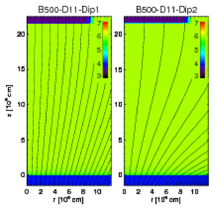
Figure 1: Temperature distribution in the $(r,z)$ plane in log scale in the simulations B500-D11-Dip1 and B500-D11-Dip2 at the initial conditions ($t=0$). The initial position of the transition region between the chromosphere and the corona is at $z=0$. The initial stellar magnetic field is oriented, on the average, along the $z$ axis and tapers close to the chromosphere; the black lines mark magnetic field lines.

The initial stellar magnetic field is assumed to be either uniform and perpendicular to the stellar surface or characterized by substantial tapering close to the chromosphere as expected by analogy with magnetic loop structures (see Fig. 1). The uniform magnetic field configuration is considered as a reference, being that used in Paper I. The nonuniform configuration is realized by assuming two identical magnetic dipoles both lying on the $z$ axis ($r=0$) and oriented parallel to it. The first dipole is located either at $z_{\mathrm{dip}}=-3\times 10^{10}$ cm or at $z_{\mathrm{dip}}=-10^{10}$ cm (see models B500-D11-Dip1 and B500-D11-Dip2 in Fig. 1); the second dipole is located specularly with respect to the upper boundary. This idealized configuration ensures magnetostaticity of the nonuniform field and the magnetic field oriented parallel to the $z$ axis at the upper boundary where we impose the inflow of the accretion stream. Such a magnetic field configuration determines a component of the field perpendicular to the flow in proximity of the chromosphere. This component may: 1) limit the overstable shock oscillations, the Lorentz force being not affected by cooling processes at variance with the force due to gas pressure (e.g. Toth & Draine 1993) and 2) limit the sinking of the shocked column in the chromosphere due to magnetic tension that is expected to sustain the hot slab. Both effects may influence the observability of the shocked plasma in the X-ray band.

From spectrometric (e.g. Johns-Krull 2007; Yang & Johns-Krull 2011) and spectropolarimetric (e.g. BP Tau, AA Tau, V2129 Oph, TW Hya, GQ Lup; Donati et al. 2008, 2010, 2011a, 2011b, 2012) observations, the inferred magnetic field strength $|\@vec{B}|$ of CTTSs is on the order of few kG. Given the stream density adopted in our simulations ($n_{\rm str0}=10^{11}$ cm^-3), we considered cases with a minimum value of magnetic field strength for which $\beta<1$ in the shocked column (namely $|\@vec{B}|=500$ G). For larger values of $|\@vec{B}|$ the evolution of the shocked plasma is not expected to change considerably, $\@vec{B}$ behaving rigidly for $\beta<1$. In all these cases, the magnetic field is able to confine and channel the shocked plasma. To investigate shocked flows only partially confined by the magnetic field, and thus perturbing the surrounding magnetic structures (see, for instance, Paper I), we considered additional simulations with $\beta$ close to or slightly larger then unity in the shocked column; for $n_{\rm str0}=10^{11}$ cm^-3, this is obtained with $|\@vec{B}|=50$ G close to the chromosphere. Although this magnetic field is quite low for a CTTS, we can investigate the dynamics of the stream impact when the shocked plasma is poorly confined because of a higher densitiy of the stream and/or because of a weaker field in the impact region.

Additional simulations with a different stream density $n_{\rm str0}$ are also considered. A summary of all the simulations discussed in this paper is given in Table 1 where: $|\@vec{B}_{\mathrm{lb}}|$ is the initial magnetic field strength at the lower boundary, $\beta_{\mathrm{slab}}$ is the average plasma $\beta$ in the hot slab, $n_{\rm str0}$, $u_{\rm str0}$, and $r_{\mathrm{str}}$ are the density, velocity, and radius of the stream at a height $z=2.1\times 10^{10}$ cm, $\dot{M}$ is the mass accretion rate, and $z_{\mathrm{dip}}$ is the position of the dipole on the $z$ axis.

In all the simulations, the 2D cylindrical $(r,z)$ mesh extends between 0 and $1.2\times 10^{10}$ cm in the $r$ direction and between $-1.4\times 10^{9}$ cm and $2.26\times 10^{10}$ cm in the $z$ direction; the transition region between the chromosphere and the corona is located at $z=0$ cm. The radial coordinate $r$ has been discretized uniformly with $N_{\mathrm{r}}=512$ points, giving a resolution of $\Delta r\approx 2.3\times 10^{7}$ cm. The coordinate $z$ has been discretized on a nonuniform grid with the mesh size increasing with $z$, giving a higher spatial resolution closer to the stellar chromosphere. The $z$-grid is made of $N_{\mathrm{z}}=896$ points and consists of: i) a uniform grid patch with 512 points and a maximum resolution of $\Delta z\approx 5.4\times 10^{6}$ cm covering the chromosphere and the upper stellar atmosphere up to the height of $\approx 3\times 10^{9}$ cm, and ii) a stretched grid patch for $z>3\times 10^{9}$ cm with the mesh size increasing with $z$ leading to a minimum resolution of $\Delta z\approx 5\times 10^{7}$ cm close to the upper boundary. This nonuniform mesh allows us to describe appropriately the steep temperature gradient of the transition region and the evolution of the hot slab of shock-heated material resulting from the impact of the accretion stream with the stellar chromosphere. The boundary conditions are the same adopted in Paper I: axisymmetric boundary conditions at $r=0$ (i.e. along the symmetry axis of the problem), free outflow at $r=1.2\times 10^{10}$ cm, fixed boundary conditions at $z=-1.4\times 10^{9}$ cm (imposing zero material and heat flux across the boundary), and a constant inflow in the upper boundary at $z=2.26\times 10^{10}$ cm.

3 Results

3.1 The reference case: uniform magnetic field

The case of uniform ambient magnetic field is considered here as a reference. As discussed below, the evolution of the accretion shock and of the post-shock plasma is analogous to that described in Paper I when the magnetic field is weak ($\beta\,\lower 4.0pt\hbox{${\buildrel\displaystyle>\over{\sim}}$}\,1$ in the post-shock plasma; run B50-D11-Unif) and to that described by Sacco et al. (2010) in the limit of strong magnetic field ($\beta\ll 1$; run B500-D11-Unif).

Figure 2 shows maps of temperature, density, and $\beta$ for runs B50-D11-Unif and B500-D11-Unif at the labeled times. Movies showing the complete evolution of 2D spatial distributions of mass density (on the left) and temperature (on the right) in log scale are provided as on-line material. In both runs, the accreting plasma flows along the magnetic field lines and impacts onto the chromosphere at $t\approx 400$ s. After the impact, a hot slab ($T\approx 5$ MK) forms at the base of the stream; the slab is partially rooted in the chromosphere so that part of the shocked material is buried under a column of material that may be optically thick. The slab is thermally unstable and quasi-periodic oscillations of the shock position are induced by radiative cooling.

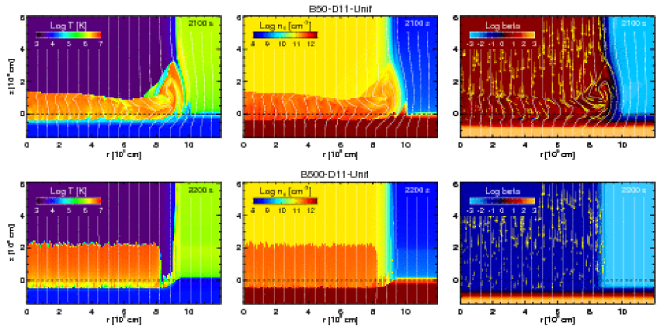
Figure 2: Temperature (left panels), plasma density (center panels), and plasma $\beta$ (right panels) distributions in the $(r,z)$ plane in log scale in the simulations B50-D11-Unif (upper panels) and B500-D11-Unif (lower panels) at the labeled times. The initial position of the transition region between the chromosphere and the corona is at z = 0 (dashed line). The initial magnetic field is uniform and oriented along the $z$ axis; the white lines mark magnetic field lines. The yellow arrows in the right panels map the velocity field.

In run B50-D11-Unif, $\beta\,\lower 4.0pt\hbox{${\buildrel\displaystyle>\over{\sim}}$}\,1$ in the slab except at the stream border where $\beta\ll 1$ (see upper right panel in Fig. 2). The post-shock plasma therefore is confined efficiently by the magnetic field (no accreting material escapes sideways) and complex 2D plasma structures form in the slab interior due to thermal instabilities. The evolution of this simulation is analogous to that of run By-50 of Paper I and we refer the reader to that case for more details. In run B500-D11-Unif, the plasma $\beta$ is $\ll 1$ in the slab. As a consequence, the stream results to be structured in several fibrils, each independent from the others. The strong magnetic field prevents mass and energy exchanges across magnetic field lines (see also Matsakos et al. 2013) and the formation of complex 2D plasma structures in the slab interior as in run B50-D11-Unif. Time-dependent 1D models as those presented by Sacco et al. (2010) describe each of these fibrils.

The global time evolution of runs B50-D11-Unif and B500-D11-Unif can be analyzed through the time-space plots of the temperature evolution. As described in Paper I, from the 2D spatial distributions of temperature and mass density, we first derive the profiles of temperature along the $z$-axis at each time $t$, by averaging the emission-measure-weighted temperature along the $r$-axis. Then the time-space plot of temperature evolution is derived from these profiles. The result is shown in Fig. 3. In the two cases considered, the hot slab penetrates the chromosphere down to the position at which the ram pressure of the post-shock plasma equals the thermal pressure of the chromosphere. As expected, the slab is not steady and its height oscillates with a period of $\approx 500$ s due to intense radiative cooling at the base of the slab (see Paper I for a detailed description of the system evolution). The maximum height reached is $D_{\mathrm{slab}}\approx 3\times 10^{9}$ cm in run B500-D11-Unif and $D_{\mathrm{slab}}\approx 2.5\times 10^{9}$ cm in run B50-D11-Unif; in the latter case the amplitude of the oscillations gradually decreases in the first 1500 s of evolution, and then stabilizes to $D_{\mathrm{slab}}\approx 2\times 10^{9}$ cm. The oscillations are more regular in run B500-D11-Unif than in B50-D11-Unif because in the latter case the dynamics of the slab is perturbed by the evolution of post-shock plasma at the stream border (see Fig. 2).

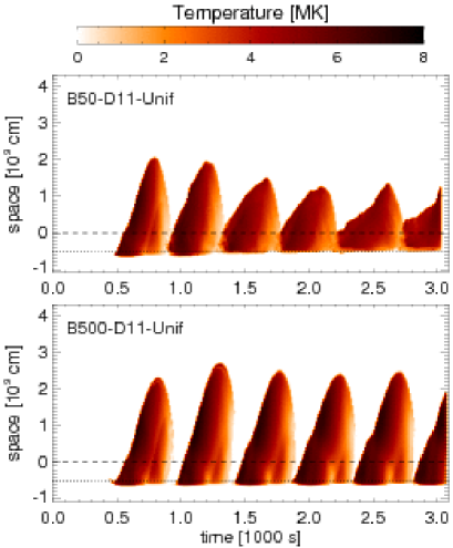
Figure 3: Time-space plots of the emission-measure-weighted temperature evolution for runs B50-D11-Unif and B500-D11-Unif. The spatial extent of the post-shock plasma in the $z$ direction lies in the vertical direction at any time. The dashed line marks the initial position of the transition region between the chromosphere and the corona; the dotted line marks the minimum sinking of the slab into the chromosphere in runs B50-D11-Unif and B500-D11-Unif.

3.2 Nonuniform magnetic field

Here we explore how a nonuniform magnetic configuration/topology influences the dynamics of the shock-heated plasma. In particular, we investigate the case of $\beta$ increasing from the chromosphere to the upper atmosphere. Figures 4 and 5 show the spatial distribution of temperature, density, and $\beta$ for different strengths and configurations of the initial magnetic field. Movies showing the complete evolution of 2D spatial distributions of mass density (on the left) and temperature (on the right) in log scale are provided as on-line material. As in the reference case of uniform magnetic field (runs B50-D11-Unif and B500-D11-Unif), the stream impact produces a shock that heats the plasma to few millions degrees (up to $\approx 5$ MK); in all the cases, $\@vec{B}$ confines efficiently the post-shock plasma. At variance with the case of uniform $\@vec{B}$, however, the field tapering makes the stream width decrease progressively (up to a factor of $\sim 5$ in run B500-D11-Dip2) and consequently the stream density increase (up to a factor of $\sim 10$ in run B500-D11-Dip2) while approaching the chromosphere.

When the stellar magnetic field is weak ($\sim 50$ G close to the chromosphere), the evolution of the shock-heated plasma is in some ways similar to that described in Sect. 3.1: a slab of hot plasma forms at the base of the accretion column and is characterized by $\beta\,\lower 4.0pt\hbox{${\buildrel\displaystyle>\over{\sim}}$}\,1$ (runs B50-D11-Dip1 and B50-D11-Dip2 in the upper panels of Figs. 4 and 5). At variance with the uniform field case, however, a large component of $\@vec{B}$ perpendicular to the stream velocity ($B_{\mathrm{r}}\approx 10|\@vec{B}_{\mathrm{0}}|$, where $\@vec{B}_{\mathrm{0}}$ is the unperturbed magnetic field) develops at the base of the hot slab (see upper panels of Figs. 4 and 5). This field component contributes to make the motion of the shock-heated plasma chaotic and to slightly perturb the overstable oscillations of the shock. The plasma velocities in the slab range between 50 and 200 km s^-1, namely on the same order of subsonic turbulent velocities measured from the line profile analysis of Ne IX in the CTTS TW Hydrae (Brickhouse et al. 2010).

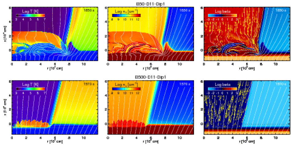
Figure 4: As in Fig. 2 for the simulations B50-D11-Dip1 (upper panels) and B500-D11-Dip1 (lower panels).

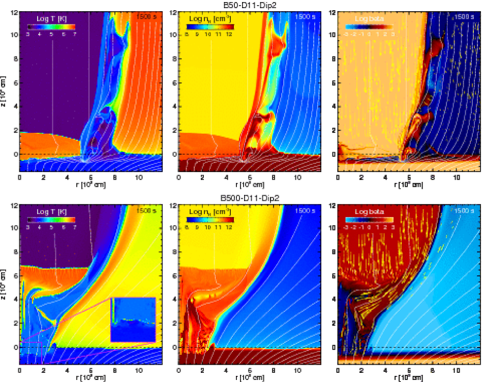
Figure 5: As in Fig. 2 for the simulations B50-D11-Dip2 (upper panels) and B500-D11-Dip2 (lower panels). The inset in the lower left panel shows the shock forming because of the stream impact onto the chromosphere.

The perpendicular field component also provides an additional magnetic pressure at the base of the stream (see Fig. 6) which limits the sinking of the slab into the chromosphere. This is shown in the upper panels of Figs. 7 and 8, the time-space plots of temperature evolution for runs B50-D11-Dip1 and B50-D11-Dip2, respectively: the slab appears less buried in the chromosphere (or even above the chromosphere in run B50-D11-Dip1) than in the uniform field case (see the dotted lines in the figure representing the minimum sinking of the slab into the chromosphere in cases with uniform $\@vec{B}$). Interestingly Ardila et al. (2013) found no evidence of the post-shock becoming buried in the stellar chromosphere from the analysis of C IV line profiles for a sample of CTTSs. Although our result largely depends on the level of complexity of the impact region and on the location of the plasma component from which the emission arises, our model suggests that the bending of magnetic field lines at the base of the accretion column might also be considered in the interpretation of the observations.

Since the hot slab is less deep in the chromosphere, the X-ray emission from the post-shock plasma should be less absorbed by the optically thick chromosphere in the presence of magnetic field tapering. However, if the field tapering is large enough (e.g. run B50-D11-Dip2), the perpendicular component of the magnetic field at the base of the stream is stronger and more steady and stable. The resulting excess magnetic pressure, therefore, is able to push chromospheric material sideways along the magnetic field lines to the upper atmosphere (see lower panel of Fig. 6); in this case, a sheath of dense and cold chromospheric material progressively grows around the stream during the accretion (see upper panels of Fig. 5). As a consequence, the shock-heated plasma may be totally enveloped by this optically thick material providing further absorption of emission from the impact region. Note that no sheath develops in run B50-D11-Dip1 because the magnetic field at the base of the stream is much more chaotic, thus preventing a laminar flow as in run B50-D11-Dip2 (see upper panels of Figs. 4 and 6, and the on-line movie); as a consequence, the cold and dense plasma at the base of the stream is not efficiently channeled by the magnetic field outwards to the upper atmosphere, remaining mostly trapped at the stream base.

When the magnetic field is strong ($\sim 500$ G close to the chromosphere), $\@vec{B}$ is not significantly perturbed by the stream (at least at the base of the corona) and the plasma flows along the magnetic field lines before impacting onto the chromosphere (see lower panels in Figs. 4 and 5). In this case the initial configuration of $\@vec{B}$ turns out to be crucial in determining the structure, geometry, and location of the shock-heated plasma. If the magnetic field tapering is small in the region of stream impact (runs B500-D10.7-Dip1 and B500-D11-Dip1 in Table 1), the hot slab forms at the base of the accretion column (as in the uniform field case) and is structured as a bundle of independent fibrils, each of them describable in terms of 1D models (see lower panels in Fig. 4). However, as already discussed, the field tapering causes the stream to squeeze and, consequently, to get denser than for a uniform magnetic field close to the chromosphere. As a result the height of the hot slab, which depends inversely on the stream density (e.g. Sacco et al. 2010), is much smaller than that in the case of uniform $\@vec{B}$ (cfr. Fig. 2). This is evident by comparing run B500-D11-Dip1 with run B500-D11-Unif (see the time-space plots of temperature evolution in Figs. 3 and 7). We note that, in run B500-D11-Dip1 only a very small portion of the slab emerges above the optically thick chromosphere. We expect therefore that the extent of chromospheric absorption in identical streams can be very different if the streams impact in regions characterized by different configurations of the stellar magnetic field.

Note that, by reducing the initial stream density in order to match the density value of run B500-D11-Unif close to the chromosphere, the fibrils have stand-off heights and evolution analogous to those of run B500-D11-Unif (see center panel in Fig. 7 for run B500-D10.7-Dip1); however, the mass accretion rate for this stream is lower than that of run B500-D11-Unif (see Tab. 1). In the case of denser accretion streams (leading to higher mass accretion rates), the evolution of the shocked plasma is expected to be similar to that of run B500-D11-Dip1 if still $\beta<1$ in the shocked slab (namely if $n_{\rm str0}<5\times 10^{12}$ cm^-3 in the case of $|\@vec{B}|=500$ G, assuming a temperature of the hot slab $T\approx 5$ MK): the plasma flows along the magnetic field lines and forms independent fibrils. In these cases, however, the shocked slab should be buried more deeply in the chromosphere, due to the larger ram pressure, and its thickness should be smaller than in run B500-D11-Dip1 (see Eq. 9 in Sacco et al. 2010). On the other hand, if the stream is so dense that $\beta\,\lower 4.0pt\hbox{${\buildrel\displaystyle>\over{\sim}}$}\,1$ in the shocked slab (this occurs, for instance, if $n_{\rm str0}>5\times 10^{12}$ cm^-3 in the case of $|\@vec{B}|=500$ G), the evolution of the post-shock plasma is expected to be more similar to that of run B50-D11-Dip1: the downfalling plasma bends the magnetic field lines, generating a large component of $\@vec{B}$ perpendicular to the stream at the base of the accretion column. Again, however, the shocked slab should be deeply buried in the chromosphere due to the high values of stream density. For these heavy streams, the X-ray emitting shocks are expected to be hardly visible in X-rays due to strong absorption by the thick chromosphere and, possibly, by the dense stream itself.

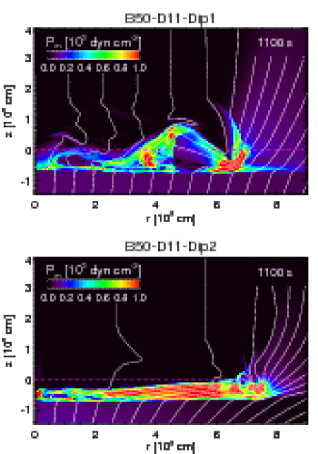
Figure 6: Maps of magnetic pressure $P_{\mathrm{m}}$ in the $(r,z)$ plane in the simulations B50-D11-Dip1 and B50-D11-Dip2 at the labeled times. The initial position of the transition region between the chromosphere and the corona is at z = 0 (dashed magenta lines). The white lines mark magnetic field lines.

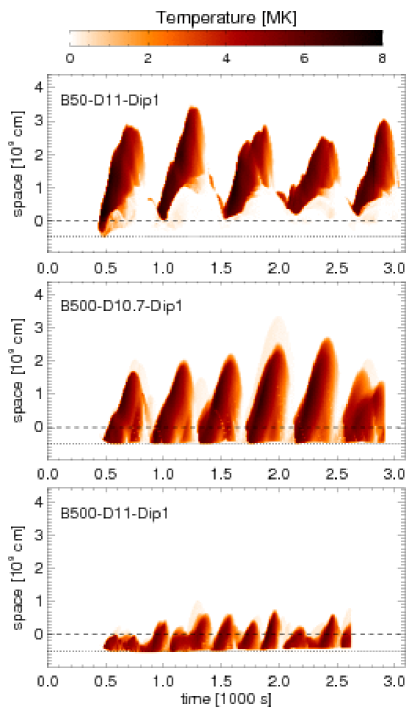
Figure 7: As in Fig. 3 for the simulations B50-D11-Dip1, B500-D10.7-Dip1, and B500-D11-Dip1.

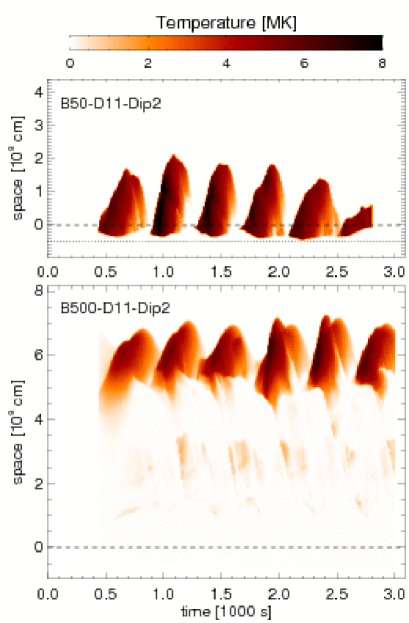
Figure 8: As in Fig. 3 for the simulations B50-D11-Dip2 and B500-D11-Dip2.

The evolution of the shock-heated material can be significantly different if $\beta$ varies strongly from the chromosphere to the upper atmosphere (runs B500-D10.7-Dip2 and B500-D11-Dip2 in Table 1). Movies showing the evolution of these runs are provided as on-line material. An example is shown in the lower panels of Fig. 5. In this case, an oblique shock forms at the height where the plasma $\beta\approx 1$ ($z\approx 6\times 10^{9}$ cm). There, the stream is well confined by the magnetic field and the downfalling plasma flows supersonically along the field lines. Due to the significant field tapering, the slope of the lines with respect to the $z$ axis gently increases to above a critical value. At that point an oblique shock forms in order to deflect the angle of the flow such that the plasma continues to flow parallel to the field lines. The oblique shock forms close to the stream border (far from the axis) where the field inclination is larger (see on-line movies). Then the shock propagates towards the stream axis where it is reflected. The on-line movies show that the shock front propagates back and forth between the site where the oblique shock forms and the symmetry axis, leading to the formation of an extended hot slab as shown in Fig. 5. The post-shock plasma can be locally thermally unstable with overstable shock oscillations induced by radiative cooling. These oscillations are evident in the time-space plot of temperature evolution (see lower panel of Fig. 8). In the slab, $\beta\,\lower 4.0pt\hbox{${\buildrel\displaystyle>\over{\sim}}$}\,1$ and the evolution of the shock-heated plasma is analogous to that described in run B50-D11-Unif. It is worth to emphasize that, at variance with all the other cases investigated in this paper, a slab of plasma with temperature of a few millions degrees forms well above the chromosphere at $z\approx 6\times 10^{9}$ cm (see lower panels of Figs. 5 and 8). Below the slab, the plasma flows along the magnetic field lines with velocities ranging between 200 and 300 km s^-1, and impacts onto the chromosphere, producing a second shock (see the inset in the lower left panel of Fig. 5). However, given the high density ($n\approx 10^{12}$ cm^-3) and low velocity ($u\approx 300$ km s^-1) of the plasma before the impact, the stand-off height of the second shock is very small and the post-shock plasma results to be fully buried in the chromosphere (thus strongly absorbed).

Note that, assuming the same strength and configuration of the magnetic field, the oblique shock forms at different heights in streams with different densities: the denser the stream, the closer to the chromosphere the oblique shock forms. On the other hand, Sacco et al. (2010) have shown that the denser the stream, the smaller the thickness of the shocked slab, due to the larger efficiency of the radiative losses. In the case of heavy streams, therefore, we expect that the post-shock plasma is located very close to the chromosphere (possibly even buried in it) and with a very small stand-off height. In these cases, therefore, the absorption by optically thick material is expected to play an important role.

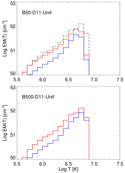
Figure 9: Distributions of emission measure vs. temperature, averaged over 3 ks, for runs B50-D11-Unif and B500-D11-Unif. Red (blue) lines mark the average EM$(T)$ distributions derived for the whole slab (for the portion of the slab emerging above the chromosphere). The dashed black line in the upper panel marks the average EM$(T)$ distribution of the whole slab for run B500-D11-Unif.

3.3 Distributions of emission measure vs. temperature

From the models we derive the distributions of emission measure vs. temperature EM$(T)$ of the shock-heated material (see Paper I for details). As shown, for instance, by Argiroffi et al. (2009), these distributions allow straightforwardly to compare the model results with the observations of accretion shocks in CTTSs. Figure 9 shows the EM$(T)$ distributions averaged over 3 ks (i.e. the total time simulated) for runs B50-D11-Unif and B500-D11-Unif. The figure shows the EM$(T)$ distributions of the whole slab (red lines) and of the portion of the slab emerging above the chromosphere (blue lines). The latter distributions show the fraction of post-shock plasma that is not buried in the optically thick chromosphere and, therefore, whose X-ray emission is expected to be less absorbed. In all the cases, we find that the EM$(T)$ has a peak at $\approx 5$ MK and a shape compatible with those derived from observations of CTTSs and attributed to plasma heated by accretion shocks (e.g. Argiroffi et al. 2009).

Figures 10 and 11 show the EM$(T)$ distributions averaged over 3 ks of the models with a tapering of the stellar magnetic field. These distributions have a shape similar to that obtained for a uniform magnetic field with a peak around $5-6$ MK. However, in all these cases, the emission measure EM is lower than that of run B500-D11-Unif (compare red lines with dashed black lines), although all these models are characterized by the same mass accretion rate ($\dot{M}\approx 5\times 10^{-11}\,M_{\mathrm{\odot}}$ yr^-1). The difference of EM is the largest at the highest temperature (above $10^{6}$ K) where the EM can be significantly lower than that of run B500-D11-Unif. On the other hand, in general, the difference decreases at lower temperatures and, in some cases, the EM can be even slightly higher than that of run B500-D11-Unif at temperatures below $10^{6}$ K (see, for instance, runs B50-D11-Dip1 and B500-D11-Dip2 in Figs. 10 and 11). As a result, we expect that the emission of the accretion shock is significanlty reduced in the X-ray band, and only slightly affected in UV and optical bands. The reduction of emission measure at high temperatures is larger when the magnetic field is weak (runs B50-D11-Dip1 and B50-D11-Dip2). In fact, in the presence of a nonuniform magnetic field, part of the kinetic energy of the stream is spent in bending the magnetic field lines during the whole evolution (see, for instance, on-line movies for runs B50-D11-Dip1 and B50-D11-Dip2) and in producing sheaths of dense and cold chromospheric material enveloping the accretion column (e.g. run B50-D11-Dip2). In the presence of a strong nonuniform field, the plasma flow slightly bends the magnetic field lines; however, the field tapering causes the stream to squeeze and to get denser, resulting in an EM($T$) distribution peaking at slightly lower temperatures with a steeper ascending slope (see Sacco et al. 2010) as found in run B500-D11-Dip1 (see Fig. 10). Note that, in run B500-D11-Dip2, the contribution to the EM$(T)$ distribution comes almost entirely from the oblique shock at $z\approx 6\times 10^{9}$ cm rather than from the shock at the region of stream impact onto the chromosphere (see the inset in the lower left panel of Fig. 5).

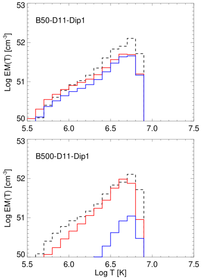
Figure 10: As in Fig. 9 for the simulations B50-D11-Dip1 and B500-D11-Dip1.

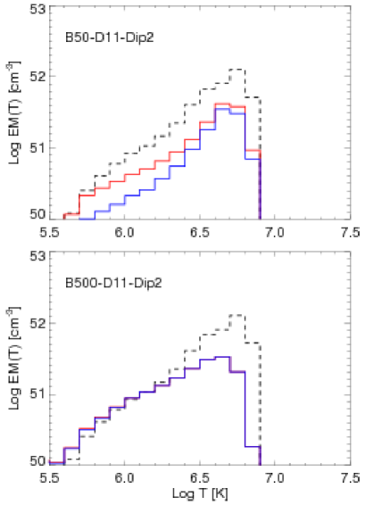
Figure 11: As in Fig. 9 for the simulations B50-D11-Dip2 and B500-D11-Dip2. Note that the blue and red diagrams are almost coincident in run B500-D11-Dip2.

The amount of post-shock plasma above the chromosphere can be very different depending on the configuration and strength of the magnetic field. In the case of weak $\@vec{B}$, most of the shock-heated plasma is above the chromosphere ($\approx 80$% for run B50-D11-Dip1 and $\approx 75$% for run B50-D11-Dip2; see upper panels in Figs. 10 and 11), thanks to the large component of $\@vec{B}$ perpendicular to the stream velocity developed at the base of the hot slab which limits the sinking of the shocked column in the chromosphere. In the case of strong $\@vec{B}$, the fraction of post-shock plasma above the chromosphere strongly depends on the amount of tapering of the magnetic field, ranging between 10% for run B500-D11-Dip1 (lower panel of Fig. 10) and 99% for run B500-D11-Dip2 (lower panel of Fig. 11). In the former case, the hot slab is buried in the chromosphere and its stand-off height allows only a small portion of the post-shock material to emerge. In the latter case, most of the shock-heated plasma originates from the oblique shock which forms well above the chromosphere. The configuration and strength of the magnetic field therefore contribute in determining the geometry and location of the shocked plasma and are expected to influence the absorption of the X-ray emitting plasma by the optically thick material surrounding the hot slab.

It is worth noting that, although the EM$(T)$ distributions of the portion of the slab emerging above the chromosphere may give a rough idea of the possible effect of the absorption on the X-ray emission (assuming that the emission from plasma below the unperturbed chromosphere is totally absorbed), they do not take into account some important effects: 1) the absorption by the cold and dense material from the unperturbed stream above the hot slab and from the perturbed chromosphere that may surround the slab; 2) the dependence of the absorption on the wavelength; 3) the point of view from which the impact region is observed, determining the distribution of thick material along the line of sight and, therefore, the absorption. To evaluate accurately the effects of absorption on the emerging X-ray emission, therefore, it is necessary to synthesize the emission taking into account all the above points. This issue will be investigated in detail in a forthcoming paper (Bonito et al. in preparation).

4 Summary and conclusions

We investigated the stability and dynamics of accretion shocks in CTTSs in a nonuniform stellar magnetic field, considering different configurations and strengths of the magnetic field. Our analysis is mainly focussed on stream impacts able to produce detectable X-ray emission. We used a 2D axisymmetric MHD model describing the impact of a continuous accretion stream onto the chromosphere of a CTTS, simultaneously including the magnetic field, the radiative cooling, and the magnetic-field-oriented thermal conduction. Our findings lead to the following conclusions.

• If the plasma $\beta\,\lower 4.0pt\hbox{${\buildrel\displaystyle>\over{\sim}}$}\,1$ where the stream hits the chromosphere (runs B50-D11-Dip1 and B50-D11-Dip2), the downfalling plasma bends the magnetic field lines thus generating a large component of $\@vec{B}$ perpendicular to the stream at the base of the accretion column. The perpendicular component limits the sinking of the slab into the chromosphere and perturbs the overstable oscillations of the shock. As a result, the fraction of the hot slab emerging above the chromosphere can be significantly larger than for a uniform magnetic field. If the tapering of the magnetic field close to the chromosphere is large, a sheath of dense and cold chromospheric material may also envelope the accretion column and the hot slab (run B50-D11-Dip2).

• If the magnetic field is strong enough to confine the downfalling plasma and guide it towars the chromosphere ($\beta<1$), the configuration of $\@vec{B}$ determines the position of the shock and its stand-off height (e.g. runs B500-D11-Dip1 and B500-D11-Dip2). In the case of a small tapering of $\@vec{B}$ close to the chromosphere (runs B500-D11-Dip1 and B500-D10.7-Dip1), a shock develops at the base of the accretion column. However, because of the decrease of the stream width (due to the tapering) and consequent increase of stream density, the stand-off height of the shock and the fraction of the hot slab emerging above the chromosphere can be much smaller than that for a uniform magnetic field.

• If the tapering of the magnetic field is large (runs B500-D11-Dip2 and B500-D10.7-Dip2), an oblique shock may form well above the chromosphere at the height where the plasma $\beta\approx 1$. As for a shock generated by the stream impact, the oblique shock can become thermally unstable with overstable oscillations induced by radiative cooling.

• A nonuniform magnetic field makes, in general, the EM$(T)$ distributions at temperatures above $10^{5}$ K lower than in the case of a strong uniform field (run B500-D11-Unif). This effect is larger at higher temperatures ($T>10^{6}$ K) and when the magnetic field is weak (runs B50-D11-Dip1 and B50-D11-Dip2). The main reason is that, in nonuniform fields, part of the kinetic energy of the downfalling stream is spent to bend the magnetic field lines during the stream impact and to develop dense and cold structures of chromospheric material that surround or even envelop (as in run B50-D11-Dip2) the base of the accretion column.

We conclude therefore that the initial strength and configuration of the magnetic field in the region of impact of the stream with the chromosphere play an important role in determining the structure, stability, and location of the post-shock plasma. In particular, they determine the fraction of the hot slab emerging above the optically thick chromosphere and the distribution of cold and dense chromospheric material around or enveloping the shocked column. All these factors are expected to concur in determining the absorption of the X-ray emitting plasma and, possibly, in underestimating the mass accretion rates $\dot{M}$ derived from X-ray observations; this issue will be investigated in detail in a forthcoming paper (Bonito et al. in preparation). The strength and configuration of the magnetic field are expected to influence also the energy balance of the post-shock plasma, the EM at $T>10^{6}$ K being in general significantly lower than expected assuming a uniform magnetic field. On the other hand, the EM does not differ too much from that in the presence of a uniform $\@vec{B}$ at $T<10^{6}$ K, and it can be even larger than in cases with uniform $\@vec{B}$ at temperatures around $10^{5.5}$ K (e.g. runs B50-D11-Dip1 and B500-D11-Dip2). As a consequence, the accretion rates $\dot{M}$ derived from X-ray observations are again expected to be underestimated if one assumes a uniform $\@vec{B}$. The above results may contribute to explain the discrepancy between $\dot{M}$ derived from X-rays and the corresponding values derived from UV/optical/NIR observations in CTTSs (e.g. Curran et al. 2011).