Abstract

This paper invites the reader to experiment with an easy-to-use MATLAB MATLAB (2012) implementation of Metropolis integrators for Molecular Dynamics (MD) simulation Bou-Rabee and Vanden-Eijnden (2010, 2012). These integrators are analysis-based, in the sense that they can rigorously simulate dynamics along an infinitely long MD trajectory. Among explicit integrators for MD, they seem to be the only ones that satisfy the fundamental requirement of stability. The schemes can handle stiff or hard-core potentials, and are straightforward to set up, apply and extend to new situations. Potential pitfalls in high dimension are discussed, and tricks for mitigation are given.

10.3390/—— xx Received: xx / Accepted: xx / Published: xx On Metropolis Integrators for Molecular Dynamics Nawaf Bou-Rabee ^1,* nawaf.bourabee@rutgers.edu 82C80 (Primary); 82C31, 65C30, 65C05 (Secondary)

1 Introduction

Molecular Dynamics (MD) simulation refers to the time integration of Hamilton’s equations often coupled to a heat or pressure bath Allen and Tildesley (1987); Frenkel and Smit (2002); Rapaport (2004); Tuckerman (2008); Schlick (2010). From its early use in computing equilibrium dynamics of homogeneous molecular systems Rahman (1964); Verlet (1967); Alder and Wainwright (1967); Alder et al. (1970); Harp and Berne (1970); Rahman and Stillinger (1971); Stillinger and Rahman (1974); Stillinger (1980) and pico to nanoscale protein dynamics McCammon et al. (1977); Van Gunsteren and Berendsen (1977); McCammon and Karplus (1980); Van Gunsteren and Karplus (1982); Karplus and McCammon (1983); van Gunsteren and Berendsen (1990); Karplus and McCammon (2002); Case (2002); Adcock and McCammon (2006); van Gunsteren et al. (2008), the method has evolved into a general purpose tool for simulating statistical properties of heterogeneous molecular systems Kapral and Ciccotti (2005). Accessible time horizons have increased remarkably: the timeline in Figure 1 attempts to capture this nearly billion-fold improvement in capability over the last forty or so years. Near future applications include micro to milliscale simulations of biomolecular processes like protein folding, ligand binding, membrane transport, and biopolymer conformational changes Scheraga et al. (2007); Dror et al. (2012); Lane et al. (2012). In addition, atomistic MD simulations are used more sparingly in multiscale models Nielsen et al. (2004); Tozzini (2005); Clementi (2008); Sherwood et al. (2008); Weinan (2011) and rare event simulation such as the finite temperature string method and milestoning E and Vanden-Eijnden (2004); Vanden-Eijnden and Venturoli (2009a, b); E and Vanden-Eijnden (2010). Given this continuous development and generalization of MD, it is not a stretch to suppose that MD will play a transformative role in medicine, technology, and education in the twenty-first century.

In its standard form, the method inputs a random initial condition, fudge factors, physical and numerical parameters; and, outputs a long discrete path of the molecular system. Statistical quantities, like velocity correlation or mean radius of gyration, are usually computed online, i.e., as points along this trajectory are produced. MD simulation is built atop a forward Euler-like integrator that requires a single interactomic force field evaluation per step. Even though MD sounds quite simple, software implementations of MD are typically optimized for performance Brooks et al. (1983); Nelson et al. (1996); Scott et al. (1999), and as a side effect, obscure this simplicity and make it cumbersome for newcomers to learn, modify, test and propose enhancements.

Besides this steep learning curve, due to the interplay between stochastic Brownian and interatomic forces, current MD integrators are unable to stably produce long trajectories. This is a well known difficulty with explicit integrators for nonlinear diffusions Talay (2002); Higham et al. (2002); Milstein and Tretyakov (2005); Higham (2011); Hutzenthaler et al. (2012). Recently, a probabilistic solution to this problem was proposed that challenges the traditional notion that Monte-Carlo methods and MD have disjoint aims: the former strictly samples probability distributions and the latter estimates dynamics. The basic idea is to combine a standard MD integrator with a Metropolis-Hastings algorithm targeted to the Gibbs-Boltzmann distribution Akhmatskaya et al. (2009); Bou-Rabee and Vanden-Eijnden (2010, 2012). Because the scheme is a Monte-Carlo method it exactly preserves the Gibbs-Boltzmann distribution Akhmatskaya et al. (2009); Bou-Rabee and Vanden-Eijnden (2010). This important property implies numerical stability over long-time simulations. In addition, a Metropolized integrator is also accurate on finite time intervals Bou-Rabee and Vanden-Eijnden (2010), and so, even though a Metropolized integrator involves a Monte-Carlo step, its aim and philosophy are very different from Monte-Carlo methods whose only goal is to sample a target distribution with no concern for the dynamics Metropolis et al. (1953); Hastings (1970); Rossky et al. (1978); Duane et al. (1987); Horowitz (1991); Kennedy and Pendleton (2001); Liu (2008); Akhmatskaya and Reich (2008); Akhmatskaya et al. (2009); Lelièvre et al. (2010).

Motivated by these issues, this paper builds a software implementation of a ‘Metropolis integrator’ and applies it to a homogeneous molecular system. The algorithms are introduced in a step-by-step fashion. The software version of the algorithm is written in the latest version of MATLAB with plenty of comments, variables that are descriptively named, and operations that can be easily translated into mathematical expressions MATLAB (2012). Since MATLAB is widely available, this design ensures the software will be easy-to-use and cross-platform. The following MATLAB-specific file formats will be used.

(F1) MATLAB Script & Function

files are written in the MATLAB language, and can be run from the MATLAB command line without ever compiling them.

(F2) MATLAB Executable (MEX)

files are written in the ‘C’ language and compiled using the MATLAB mex function. The resulting executable is comparable in efficiency to a ‘C’ code and can be called directly from the MATLAB command line. We will use MEX-files for performance-critical routines The Mathworks Inc. .

(F3) MATLAB Binary (MAT)

files will be used to store simulation data.

The paper is organized as follows. We begin with some mathematical background in §2, followed by an algorithmic introduction to time integrators in MD simulation and a statistical analysis of a long trajectory of a Lennard-Jones fluid in §3. The paper discusses some tricks to get the integrator to scale well in high dimension in §4. We close the paper with some steps for future development of Metropolis integrators in §5.

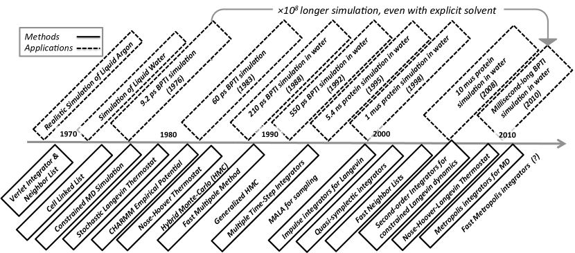
Figure 1: Timeline of Selected MD Developments. A timeline of the evolution of MD simulation methodology and applications. The applications highlighted are simulations of liquid argon Rahman (1964), water Rahman and Stillinger (1971), protein dynamics without solvent McCammon et al. (1977); Van Gunsteren and Berendsen (1977), and biopolymer dynamics with solvent Levitt (1983); Levitt and Sharon (1988); Daggett and Levitt (1992); Li and Daggett (1995); Duan and Kollman (1998); Freddolino et al. (2008); Shaw et al. (2010). The methods include the following upgrades to MD simulation: Verlet integrator and neighbor lists Verlet (1967), cell linked list Quentrec and Brot (1973), SHAKE integrator for constraints Ryckaert et al. (1977), stochastic heat baths via Langevin dynamics Schneider and Stoll (1978); Brünger et al. (1984), library of empirical potentials Brooks et al. (1983), extended/deterministic heat bath via Nosé-Hoover dynamics Nosé (1984); Hoover (1985), fast multipole method Greengard and Rokhlin (1987), multiple time-steps Tuckerman et al. (1992), Langevin splitting methods Skeel and Izaguirre (2002); Milstein and Tretyakov (2003), (fast) combined neighbor and cell lists Yao et al. (2004), second-order Langevin integrators for constrained systems Vanden-Eijnden and Ciccotti (2006), and stochastic Nosé-Hoover Langevin thermostat Samoletov et al. (2008); Leimkuhler et al. (2009); Leimkuhler and Reich (2009).

2 Mathematical Background

2.1 Bath–Free Dynamics

MD is based on Hamilton’s equations for a Hamiltonian $H:\mathbb{R}^{2d}\to\mathbb{R}$:

$$\dot{\boldsymbol{z}}(t)=\boldsymbol{J}\nabla H(\boldsymbol{z}(t))\;,~{}~{}\boldsymbol{z}(0)\in\mathbb{R}^{2d}\;,$$ (1)

where $\boldsymbol{z}(t)=(\boldsymbol{q}(t),\boldsymbol{p}(t))$ is a vector of molecular positions $\boldsymbol{q}(t)\in\mathbb{R}^{d}$ and momenta $\boldsymbol{p}(t)\in\mathbb{R}^{d}$, and $\boldsymbol{J}$ is the $2d\times 2d$ skew-symmetric matrix defined as:

$$\boldsymbol{J}=\begin{pmatrix}\boldsymbol{0}_{d\times d}&\boldsymbol{I}_{d\times d}\\ -\boldsymbol{I}_{d\times d}&\boldsymbol{0}_{d\times d}\end{pmatrix}\;.$$

The Hamiltonian $H(\boldsymbol{z})$ represents the total energy of the molecular system, and is typically ‘separable’ meaning that it can be written as:

$$H(\boldsymbol{z})=K(\boldsymbol{p})+U(\boldsymbol{q})\;,~{}~{}\boldsymbol{z}=(\boldsymbol{q},\boldsymbol{p})\;,$$

where $K(\boldsymbol{p})$ and $U(\boldsymbol{q})$ are the kinetic and potential energy functions, respectively Marsden and Ratiu (1999). In MD, the kinetic energy function is a positive definite quadratic form, and the potential energy function involves ‘fudge factors’ determined from experimental or quantum mechanical studies of pieces of the molecular system of interest Brooks et al. (1983). The accuracy of the resulting energy function must be systematically verified by comparing MD simulation data to experimental data van Gunsteren and Mark (1998). The flow that (1) determines has the following structure:

(S1)

volume-preserving (since the vector-field in (1) is divergenceless); and,

(S2)

energy-preserving (since $\boldsymbol{J}$ is skew-symmetric & constant).

Explicit symplectic integrators – like the Verlet scheme – exploit these properties to obtain long-time stable schemes for Hamilton’s equations Leimkuhler and Reich (2004); Hairer et al. (2010).

2.2 Governing Stochastic Dynamics

In order to mimic experimental conditions, (1) is often coupled to a bath that puts the system at constant temperature and/or pressure. The standard way to do this is to assume that the system with bath is governed by a stochastic ordinary differential equation (SDE) of the type:

$$\boxed{d\boldsymbol{Y}(t)=\underset{\text{deterministic drift}}{\underbrace{\boldsymbol{A}(\boldsymbol{Y}(t))dt}}+\underset{\text{heat bath}}{\underbrace{(\operatorname{div}\boldsymbol{D})(\boldsymbol{Y}(t))dt+\sqrt{2kT}\boldsymbol{B}(\boldsymbol{Y}(t))d\boldsymbol{W}(t)}}}$$ (2)

Here, we have introduced the following notation.

$\boldsymbol{Y}(t)\in\mathbb{R}^{n}$	state of the (extended) system
$\boldsymbol{A}(\boldsymbol{x})\in\mathbb{R}^{n}$	deterministic drift vector field
$\boldsymbol{B}(\boldsymbol{x})\in\mathbb{R}^{n\times n}$	noise-coefficient matrix
$\boldsymbol{D}(\boldsymbol{x})\in\mathbb{R}^{n\times n}$	diffusion matrix
$\boldsymbol{W}(t)\in\mathbb{R}^{n}$	$n$-dimensional Brownian motion
$kT$	temperature factor

The $n\times n$ diffusion matrix $\boldsymbol{D}(\boldsymbol{x})$ is defined in terms of the noise coefficient matrix $\boldsymbol{B}(\boldsymbol{x})$ as:

$$\boldsymbol{D}(\boldsymbol{x})\stackrel{{\scriptstyle\mbox{\tiny def}}}{{=}}kT\boldsymbol{B}(\boldsymbol{x})\boldsymbol{B}(\boldsymbol{x})^{T}\;,~{}~{}\text{for all $\boldsymbol{x}\in\mathbb{R}^{n}$}\;,$$ (3)

where $\boldsymbol{B}(\boldsymbol{x})^{T}$ denotes the transpose of the real matrix $\boldsymbol{B}(\boldsymbol{x})$. The diffusion matrix is symmetric and nonnegative definite. Depending on the particular bath that is used, the dimension $n$ of $\boldsymbol{Y}(t)$ in (2) is related to the dimension $2d$ of $\boldsymbol{z}(t)$ in (1) by the inequality: $n\geq 2d$. For example, in Nosé-Hoover Langevin dynamics a single bath degree of freedom is added to (1) so that $n=2d+1$, while in Langevin dynamics the effect of the bath is modeled by added friction and Brownian forces that keep $n=2d$. Throughout this work, MD simulation refers to time integration of (2) from a random initial condition.

The equations (2) generate a stochastic process $\boldsymbol{Y}(t)$ that is a Markov diffusion process. We assume that this diffusion process admits a stationary distribution $\mu(d\boldsymbol{x})$, i.e., a probability distribution preserved by the dynamics Ikeda and Watanabe (1989); Klebaner (2005). We denote by $\nu(\boldsymbol{x})$ the density of this distribution. Even though the diffusion matrix (3) is not necessarily positive definite, one can use Hörmander’s condition to prove that the process $\boldsymbol{Y}(t)$ is an ergodic process with a unique stationary distribution Mengersen and Tweedie (1996); Prato and Zabczyk (1996). By the ergodic theorem, it then follows that:

$$\frac{1}{T}\int_{0}^{T}f(\boldsymbol{Y}(t))dt\to\int_{\mathbb{R}^{n}}f(\boldsymbol{x})\nu(\boldsymbol{x})d\boldsymbol{x}\;,~{}~{}\text{as}~{}~{}T\to\infty,$$ (4)

where $f(\boldsymbol{x})$ is a suitable test function.

The evolution of the probability density of the law of $\boldsymbol{Y}(t)$ at time $t$, $\rho(t,\boldsymbol{x})$, satisfies the Fokker-Planck equation:

$$-\frac{\partial\rho}{\partial t}+L\rho=0\;,$$ (5)

where $\rho(0,\cdot)$ is the density of the initial distribution $\boldsymbol{Y}(0)\sim\rho(0,\cdot)$, and $\mathcal{L}$ is defined as the following second-order partial differential operator:

$$(Lf)(\boldsymbol{x})\stackrel{{\scriptstyle\mbox{\tiny def}}}{{=}}\operatorname{div}\left(\operatorname{div}(\boldsymbol{D}(\boldsymbol{x})f(\boldsymbol{x}))-\boldsymbol{A}(\boldsymbol{x})f(\boldsymbol{x})\right)\;.$$

Since $\mu(d\boldsymbol{x})=\nu(\boldsymbol{x})d\boldsymbol{x}$ is a stationary distribution of $\boldsymbol{Y}(t)$, the probability density $\nu(\boldsymbol{x})$ is a steady-state solution of (5):

$$(L\nu)(\boldsymbol{x})=0\;.$$ (6)

Define the probability current as the vector field:

$$\boldsymbol{j}(\boldsymbol{x})\stackrel{{\scriptstyle\mbox{\tiny def}}}{{=}}\operatorname{div}(\boldsymbol{D}(\boldsymbol{x})\nu(\boldsymbol{x}))-\boldsymbol{A}(\boldsymbol{x})\nu(\boldsymbol{x})$$ (7)

The stationarity condition (6) implies that $\boldsymbol{j}(\boldsymbol{x})$ is divergenceless. In the zero-current case, the diffusion process $\boldsymbol{Y}(t)$ is reversible and the stationary density $\nu(\boldsymbol{x})$ is called the equilibrium probability density of the diffusion Haussman and Pardoux (1986).

In this case, the operator $L$ is self-adjoint, in the sense that:

$$\langle Lf,g\rangle_{\nu}=\langle f,Lg\rangle_{\nu}\qquad\text{for all suitable test functions $f,g$}\;,$$ (8)

where $\langle\cdot,\cdot\rangle_{\nu}$ denotes an $L^{2}$ inner product weighted by the density $\nu(x)$. This property implies that the diffusion is $\nu$-symmetric Kent (1978):

$$\nu(\boldsymbol{x})p_{t}(\boldsymbol{x},\boldsymbol{y})=\nu(\boldsymbol{y})p_{t}(\boldsymbol{y},\boldsymbol{x})\qquad\text{for all $t>0$}\;,$$ (9)

where $p_{t}(\boldsymbol{x},\boldsymbol{y})$ denotes the transition probability density of $\boldsymbol{Y}(t)$. Indeed (8) is simply an infinitesimal version of (9), which is referred to as the detailed balance condition. In the self-adjoint case, the drift is uniquely determined by the diffusion matrix and the stationary density $\nu(\boldsymbol{x})$:

$$\boldsymbol{j}(\boldsymbol{x})=\boldsymbol{0}\implies\boldsymbol{A}(\boldsymbol{x})=\frac{1}{\nu(\boldsymbol{x})}\operatorname{div}(\boldsymbol{D}(\boldsymbol{x})\nu(\boldsymbol{x}))\;.$$

Long-time stable explicit schemes adapted to this structure have been recently developed Bou-Rabee et al. (2013).

2.3 Splitting Approach to MD Simulation

We are now in position to explain our approach to deriving a long-time stable scheme for (2). Crucial to our approach is that in MD simulation we usually have a formula for a function proportional to the stationary density $\nu(\boldsymbol{x})$. Following Bou-Rabee and Owhadi (2010), we can split (2) into:

$$d\boldsymbol{Y}=-\boldsymbol{D}(\boldsymbol{Y})\nabla H_{\nu}(\boldsymbol{Y})dt+\operatorname{div}\boldsymbol{D}(\boldsymbol{Y})dt+\sqrt{2kT}B(\boldsymbol{Y})dW$$ (10)

$$\dot{\boldsymbol{Y}}=\boldsymbol{A}(\boldsymbol{Y})+\boldsymbol{D}(\boldsymbol{Y})\nabla H_{\nu}(\boldsymbol{Y})$$ (11)

where we have introduced $H_{\nu}(\boldsymbol{x})=-(\log\nu)(\boldsymbol{x})$. An exact splitting method preserves $\mu(d\boldsymbol{x})$. It is formed by taking the exact solution (in law) of (10) in composition with the exact flow of (11). The process produced by (10) is self-adjoint with respect to $\nu(\boldsymbol{x})$. Moreover, stationarity of $\nu(\boldsymbol{x})$ implies that the flow of the ODE (11) preserves it. Since each step is preservative, their composition is too.

In place of the exact splitting, a Metropolis integrator can be used for (10) Bou-Rabee et al. (2013), and a measure-preserving scheme can be designed to solve the ODE Ezra (2006); Bou-Rabee and Vanden-Eijnden (2010). In Bou-Rabee et al. (2013), explicit schemes are introduced for (10) that, for the first time: (i) sample the exact equilibrium probability density of the SDE when this density exists (i.e., whenever $\nu(\boldsymbol{x})$ is normalizable); (ii) generates a weakly accurate approximation to the solution of (2) at constant $kT$; (iii) acquire higher order accuracy in the small noise limit, $kT\to 0$; and, (iv) avoid computing the divergence of the diffusion. Compared to the methods in Bou-Rabee and Vanden-Eijnden (2010), the main novelty of these schemes stems from (iii) and (iv). The resulting explicit splitting method is accurate, since it is an additive splitting of (2); and typically ergodic when the continuous process is ergodic Bou-Rabee and Vanden-Eijnden (2010).

This type of splitting of (2) is quite natural and has been used before in: MD Vanden-Eijnden and Ciccotti (2006); Bussi and Parrinello (2007), dissipative particle dynamics Shardlow (2003); Serrano et al. (2006), and simulation of inertial particles Pavliotis et al. (2008). Other related schemes for (2) include Brünger-Brooks-Karplus (BBK) Brünger et al. (1984), van Gunsteren and Berendsen (vGB) van Gunsteren and Berendsen (1982), the Langevin-Impulse (LI) methods Skeel and Izaguirre (2002), and quasi-symplectic integrators Milstein and Tretyakov (2003). The long-time statistical properties of this splitting was quantified in the context of globally Lipschitz potential forces in Bou-Rabee and Owhadi (2010). However, for general MD force fields, none of these explicit integrators are stable. Our framework to stabilize explicit MD integrators is the Metropolis-Hastings algorithm.

2.4 Metropolis-Hastings algorithm

A Metropolis-Hastings method is a Monte-Carlo method for producing samples from a probability distribution, given a formula for a function proportional to its density Metropolis et al. (1953); Hastings (1970). The algorithm consists of two sub-steps: firstly, a proposal move is generated according to a transition density $g(\boldsymbol{x},\boldsymbol{y})$; and second, this proposal move is accepted or rejected with a probability:

$$\alpha(\boldsymbol{x},\boldsymbol{y})=1\wedge\frac{g(\boldsymbol{y},\boldsymbol{x})\nu(\boldsymbol{y})}{g(\boldsymbol{x},\boldsymbol{y})\nu(\boldsymbol{x})}\;.$$ (12)

Standard results on Metropolis-Hastings methods can be used to classify this algorithm as ergodic Nummelin (1984); Tierney (1994); Mengersen and Tweedie (1996).

3 Algorithmic Introduction to MD Integrators

We now focus our discussion on Langevin dynamics of a system of $N$ atoms. Denote by $m_{j}>0$ and $\boldsymbol{q}_{j}$ the mass and position of the $j$th atom, respectively. The governing Langevin equation is given by:

$$\begin{cases}\dot{\boldsymbol{q}}_{j}(t)=m_{j}^{-1}\boldsymbol{p}_{j}(t)\;,\\ d\boldsymbol{p}_{j}(t)=-\frac{\partial U}{\partial\boldsymbol{q}_{j}}(\boldsymbol{q}(t))dt-\gamma\boldsymbol{p}_{j}(t)dt+\sqrt{2kT\gamma m_{j}}d\boldsymbol{w}_{j}\;,\end{cases}~{}~{}j=1,\cdots,N\;,$$ (13)

where $\boldsymbol{q}=(\boldsymbol{q}_{1},\cdots,\boldsymbol{q}_{N})$ and $\boldsymbol{p}=(\boldsymbol{p}_{1},\cdots,\boldsymbol{p}_{N})$ denote the positions and momenta of the particles, and $\boldsymbol{w}_{j}$ are independent Brownian motions. In Langevin dynamics, positions are differentiable, and due to the irregularity of the Brownian force, momenta are just continuous but not differentiable. The last two terms in the second equation represent the effect of the bath. The bath-free dynamics is a Hamiltonian system with:

$$H(\boldsymbol{q},\boldsymbol{p})=\sum_{j=1}^{N}\frac{1}{2m_{j}}|\boldsymbol{p}_{j}|^{2}+U(\boldsymbol{q})\;.$$

The stationary distribution of the Langevin process has the following density:

$$\nu(\boldsymbol{q},\boldsymbol{p})=Z^{-1}\exp\left(-\frac{1}{kT}H(\boldsymbol{q},\boldsymbol{p})\right)\;,~{}~{}Z=\int\exp\left(-\frac{1}{kT}H(\boldsymbol{q},\boldsymbol{p})\right)d\boldsymbol{q}d\boldsymbol{p}\;.$$ (14)

The Langevin equation (13) can be put in the form of (2) by letting $\boldsymbol{x}=(\boldsymbol{q},\boldsymbol{p})$,

$$\boldsymbol{A}(\boldsymbol{x})=\begin{pmatrix}\boldsymbol{m}^{-1}\boldsymbol{p}\\ -\nabla U(\boldsymbol{q})-\gamma\boldsymbol{p}\end{pmatrix}\;,~{}~{}\boldsymbol{B}=\sqrt{\gamma}\begin{pmatrix}\boldsymbol{0}&\boldsymbol{0}\\ \boldsymbol{0}&\boldsymbol{m}^{1/2}\end{pmatrix}\;,~{}~{}\text{and}~{}~{}\boldsymbol{W}=(\boldsymbol{w}_{1},\cdots,\boldsymbol{w}_{N})\;,$$ (15)

where $\boldsymbol{m}=\operatorname{diag}(m_{1},\cdots,m_{N})$. The splitting approach discussed in §2 applied to Langevin dynamics (13) leads to the following special cases of (10) and (11):

$$\begin{cases}d\boldsymbol{p}(t)=-\gamma\boldsymbol{p}(t)dt+\sqrt{2kT\gamma}\boldsymbol{m}^{1/2}d\boldsymbol{W}\;,\end{cases}$$ (16)

$$\begin{cases}\dot{\boldsymbol{q}}(t)=\boldsymbol{m}^{-1}\boldsymbol{p}(t)\;,\\ \dot{\boldsymbol{p}}(t)=-\nabla U(\boldsymbol{q}(t))\;.\end{cases}$$ (17)

Notice that (16) is a linear SDE that can be exactly solved (Evans, 2007, See Chapter 5). We will use a Verlet integrator for (17) that preserves volume and represents the energy to third-order accuracy per step. Since the Verlet integrator does not exactly preserve energy, the composition of the two schemes does not preserve the stationary distribution with density (14). As a consequence of this discretization error, this scheme may either not detect properly features of the potential energy, which leads to unnoticed but large errors in dynamic quantities such as the mean first passage time, or may mishandle soft or hard-core potentials, which leads to numerical instabilities; see the numerical examples in Bou-Rabee et al. (2013). These numerical artifacts motivate adding a Metropolis accept/refusal sub-step to the integrator. The corrected MD integrator follows.

Algorithm 3.1 (Analysis-based MD Integrator).

Given the current state $(\boldsymbol{Q}_{0},\boldsymbol{P}_{0})$ at time $t$ the algorithm proposes a position $(\boldsymbol{Q}_{1}^{\star},\boldsymbol{P}_{1}^{\star})$ at time $t+h$ for some time-step $h>0$ via

$$\begin{cases}\boldsymbol{P}_{1/2}=\boldsymbol{P}_{0}-\frac{h}{2}\nabla U(\boldsymbol{Q}_{0})\\ \boldsymbol{Q}_{1}^{\star}=\boldsymbol{Q}_{0}+h\boldsymbol{P}_{1/2}\\ \boldsymbol{P}_{1}^{\star}=\boldsymbol{P}_{1/2}-\frac{h}{2}\nabla U(\boldsymbol{Q}_{1}^{\star})\end{cases}$$ (Step 1)

The ‘proposal move’ $(\boldsymbol{Q}_{1}^{\star},\boldsymbol{P}_{1}^{\star})$ is then accepted or rejected:

$$\begin{pmatrix}\tilde{\boldsymbol{Q}}_{1}\\ \tilde{\boldsymbol{P}}_{1}\end{pmatrix}=x\begin{pmatrix}\boldsymbol{Q}_{1}^{\star}\\ \boldsymbol{P}_{1}^{\star}\end{pmatrix}+(1-x)\begin{pmatrix}\boldsymbol{Q}_{0}\\ -\boldsymbol{P}_{0}\end{pmatrix}\;,$$ (Step 2)

where $x$ is a Bernoulli random variable with parameter $\alpha$, i.e., it takes value 1 with probability $\alpha$ and value 0 with probability $1-\alpha$. The acceptance probability is defined as:

$$\alpha=1\wedge\exp\left(-\frac{1}{kT}(H(\boldsymbol{Q}_{1}^{\star},\boldsymbol{P}_{1}^{\star})-H(\boldsymbol{Q}_{0},\boldsymbol{P}_{0}))\right)\;.$$ (18)

The actual update of the system is taken to be:

$$\begin{pmatrix}\boldsymbol{Q}_{1}\\ \boldsymbol{P}_{1}\end{pmatrix}=\begin{pmatrix}\tilde{\boldsymbol{Q}}_{1}\\ \exp(-\gamma h)\tilde{\boldsymbol{P}}_{1}+\sqrt{1-\exp(-2\gamma h)}\boldsymbol{m}^{1/2}\boldsymbol{\xi}\end{pmatrix}\;.$$ (Step 3)

Here $\boldsymbol{\xi}\in\mathbb{R}^{n}$ denotes a Gaussian random vector with mean zero and covariance $\mathbb{E}(\boldsymbol{\xi}_{i}\boldsymbol{\xi}_{j})=kT\boldsymbol{\delta}_{ij}$.

Notice that the momentum gets flipped if a move is rejected in (Step 2). This momentum flip is necessary in order to guarantee that the algorithm samples the correct stationary distribution Akhmatskaya et al. (2009), but results in a $O(1)$ error in dynamics. To compute dynamics not only must a long trajectory be stably produced with the right stationary distribution, but the approximation must also accurately represent the system’s dynamics over the time interval of interest. Unlike sampling algorithms, high acceptance rates are needed to ensure that the time lag between successive rejections is frequently long enough to capture the desired dynamics. Since the acceptance rate in (18) is related to how well the Verlet step preserves energy after a single step, this rejection rate is $O(h^{3})$. Thus, in practice we find that the time-step required to obtain a $99.9\%$ acceptance rate is often automatically satisfied with a time-step that sufficiently resolves the desired dynamics. Each step of this algorithm requires: evaluating the atomic force field once in the third equation of (Step 1), generating a Bernoulli random variable with parameter $\alpha$ in (Step 2), and generating an $n$-dimensional Gaussian vector in (Step 3). Since (Step 3) is the exact solution of (10), we stress that (Step 2) in Algorithm 3.1 is all that is really needed in most MD integration schemes to ensure that the integrator preserves the correct stationary density (14).

Listing 1 translates Algorithm 3.1 into the MATLAB language. Intrinsically defined MATLAB functions appear in boldface. The algorithm uses MATLAB’s built in random number generators to carry out (Step 2) and (Step 3). In particular, the Bernoulli random variable $x$ in (Step 2) is generated in Line 15, and the Gaussian vector in (Step 3) is generated on Line 24. In addition to updating the positions and momenta of the system, the program also stores the previous value of the potential energy and force, so that the force and potential energy is evaluated just once in Line 12 per simulation step. This evaluation calls a MEX function which inputs the current position of the molecular system and outputs the force field and potential energy at that position. We use a MEX function because the atomistic force-field evaluation cannot be easily vectorized, and is by far, the most computationally demanding step in MD. The PreProcessing script file called in Line 2 defines the physical and numerical parameters, sets the initial condition, and allocates space for storing simulation data. Sample averages are updated as new points on the trajectory are produced in the UpdateSampleAverages script file invoked in Line 30. Finally, the outputs produced by the algorithm are handled by the PostProcessing script file in Line 34.

Listing 1: Analysis-Based MD Integrator: MDintegrator.m

⬇

1

2PreProcessing;

3

4for i = 1:Ns

5

6 %--- Step 1 --- Velocity Verlet Proposal

7

8 Ppt5=P0+0.5*h*F0;

9 Q1star=Q0+h*Ppt5;

10 [F1star,U1star]=ForceFieldmex(Q1star,Nm,rcut2,ell);

11 P1star=Ppt5+0.5*h*F1star;

12

13 %--- Step 2 --- Accept or Refuse Step

14

15 x=(rand<exp(-(0.5*P1star’*P1star-0.5*P0’*P0+U1star-U0)/kT));

16

17 tildeP1=x*P1star-(1-x)*P0;

18 tildeQ1=x*Q1star+(1-x)*Q0;

19 F1=x*F1star+(1-x)*F0; U1=x*U1star+(1-x)*U0;

20

21 %--- Step 3 --- Heat Bath Step

22

23 Q1=tildeQ1;

24 P1=f1*tildeP1+f2*randn(3*Nm,1);

25

26 %--- iterate

27

28 Q0=Q1; P0=P1; F0=F1; U0=U1;

29

30 UpdateSampleAverages;

31

32end

33

34PostProcessing;

Let us consider a concrete example: a Lennard-Jones fluid that consists of $N$ identical atoms Allen and Tildesley (1987); Frenkel and Smit (2002); Rapaport (2004). The configuration space of this system is a fixed cubic box with periodic boundary conditions. The distance between the ith and jth particle is defined according to the minimum image convention, which states that the distance between $\boldsymbol{q}_{i}$ and $\boldsymbol{q}_{j}$ in a cubic box of length $\ell$ is:

$$d_{MD}(\boldsymbol{q}_{i},\boldsymbol{q}_{j})\stackrel{{\scriptstyle\mbox{\tiny def}}}{{=}}|(\boldsymbol{q}_{i}-\boldsymbol{q}_{j})-\ell\lfloor(\boldsymbol{q}_{i}-\boldsymbol{q}_{j})/\ell\rceil|\;.$$ (19)

where $\lfloor\cdot\rceil$ is the nearest integer function. In terms of this distance, the total potential energy is a sum over all pairs:

$$U(\boldsymbol{q})=\sum_{i=1}^{n-1}\sum_{j=i+1}^{n}U_{LJ}(d_{MD}(\boldsymbol{q}_{i},\boldsymbol{q}_{j}))\;,$$ (20)

where $U_{LJ}(r)$ is the following truncated Lennard-Jones potential function:

$$U_{LJ}(r)=\begin{cases}f(r)-f(r_{c})&r<r_{c}\;,\\ 0&\text{otherwise}\;.\end{cases}$$ (21)

Here, $f(r)=4(1/r^{12}-1/r^{6})$ and $r_{c}$ is the cutoff radius which is bounded above by the size of the simulation box; and we have used dimensionless units to describe this system, where energy is rescaled by the depth of the Lennard-Jones potential energy and length by the point where the potential energy is zero. The error introduced by the truncation in (21) is proportional to the density of the molecular system and can be made arbitrarily small by selecting the cutoff distance sufficiently large. Unless a neighbor and/or cell list is employed, a direct evaluation of the potential force $\nabla U(\boldsymbol{q})$ scales like $O(N^{2})$, and typically dominates the total computational cost Yao et al. (2004). Since the molecular system we consider will have just a few hundred atoms, we found that there is no advantage to using a fast force–field evaluation, and thus ForceFieldmex evaluates the force and energy using a sum over all particle pairs.

Parameter	Description	Value
Physical Parameters
$\rho$	density	$\{0.6,0.7,0.8,0.9,1.0,1.1\}$
$kT$	temperature	$0.5$
$\gamma$	heat bath parameter	$0.01$
$N_{m}$	# of molecules	$512$
$T$	time-span for autocorrelation	$2$
Numerical Parameters
$h$	time-step	$0.005$
$N_{s}$	# of simulation steps	$10^{5}$
$r_{c}$	LJ cutoff radius	$2^{1/6}$

Table 1: Simulation Parameters.

Listing 2 shows the PreProcessing script which sets the parameters provided in Table 1 and constructs the initial condition, where the $N$ atoms are assumed to be at rest and on the sites of an FCC lattice. The command rng(123) on Line 3 sets the seed of the random number generator functions RAND and RANDN. The acceptance rates at every step and the velocity autocorrelation are updated in the UpdateSampleAverages script shown in Listing 3. The mean acceptance rate which is outputted in the script PostProcessing shown in Listing 4 must be high enough to ensure that the dynamics is accurately represented. To compute the autocorrelation of an observable over a time interval of length $T$, the value of that observable along the entire trajectory is not needed. In fact, all that is really needed are the values of this observable along a piece of trajectory over the moving time-window $[t_{i},t_{i}+T]$ where $t_{i}=i\times h$. This storage space is allocated in PreProcessing and is updated in UpdateSampleAverages. More precisely, since we define $N_{a}=\lceil T/h\rceil+1$ in the PreProcessing script, the molecular velocities are stored in the pivot array from $i-N_{a}$ to $i$, where $i$ is the index of the current position. Notice that velocity autocorrelations are not computed until after the index $i$ exceeds $10^{4}$. This equilibration time removes some of the statistical bias that may arise from using a non-random initial condition. Short-time trajectories of this molecular system are plotted in Figure 2. This figure shows that the particle motions are more localized at higher densities. Using the parameters provided in Table 1, we compute velocity autocorrelations for a range of density values in Figure 3. Since the heat bath parameter is set to a small value, these figures are in agreement with those obtained by simulating the molecular system with no heat bath in Figure 5.2 of Rapaport (2004).

Listing 2: Analysis-Based MD Integrator: PreProcessing.m

⬇

1%--- seed random # generator

2

3rng(123);

4

5%--- physical parameters

6

7rho=0.6; % density

8kT=0.5; % temperature factor

9gama=0.1; % heat bath parameter

10Nm=500; % # of molecules

11T=2.0; % time span for velocity correlation

12ell=(Nm/rho)^(1/3); % length of cubic box

13

14%--- simulation parameters

15

16h=0.005; % time-step size

17Ns=1e3; % # of steps

18rcut = 2.0^(1/6); % cutoff radius

19rcut2 = rcut*rcut;

20

21f1=exp(-gama*h); f2=sqrt((1.0-exp(-2.0*gama*h))*kT);

22

23%--- initial condition

24

25A=fcclattice(Nm,ell);

26Q0=reshape(A, [3*Nm 1]); % atoms on an fcc lattice

27P0=zeros(3*Nm,1); % atoms at rest

28

29%--- initialize statistics

30

31NA=ceil(T/h)+1; % preallocate space for

32acf=zeros(NA,1); % online correlation computation

33varacf=zeros(NA,1);

34pivot=zeros(NA,3*Nm);

35nacf=zeros(NA,1);

36

37AP=zeros(Ns,1); % vector of acceptance probabilities

38

39[F0,U0]=ForceFieldmex(Q0,Nm,rcut2,ell); % initial force & energy

Listing 3: Analysis-Based MD Integrator: UpdateSampleAverages.m

⬇

1%--- store acceptance probability

2

3AP(i)=x;

4

5%--- update correlation function

6

7if (i>1e4)

8

9 pp=mod(i-1,NA)+1;

10 pivot(pp,:)=P0;

11

12 for j=1:min(i,NA)

13 nacf(j)=nacf(j)+1;

14 mui=acf(j);

15 vari=varacf(j);

16 n_samples=nacf(j);

17 xip1=pivot(mod(pp-j,NA)+1,:)*pivot(pp,:)’/(3.0*Nm);

18␣␣␣␣␣␣␣␣acf(j)=mui+(xip1-mui)/n_samples;

19␣␣␣␣␣␣␣␣varacf(j)=((n_samples-1)*vari+...

20␣␣␣␣␣␣␣␣␣␣␣␣(xip1-mui)*(xip1-acf(j)))/n_samples;

21␣␣␣␣end

22

23end

Listing 4: Analysis-Based MD Integrator: PostProcessing.m

⬇

1%--- output results

2

3disp([’h=’␣num2str(h)␣␣’,<AP>=’␣num2str(mean(AP))]);

4

5figure(2);␣clf;␣hold␣on;␣tt=0:h:T;

6errorbar(tt,acf,1.96*sqrt(varacf)./sqrt(nacf));

7

8save(’VelocityAutocorrelation.mat’,␣’tt’,␣’acf’,␣’varacf’);

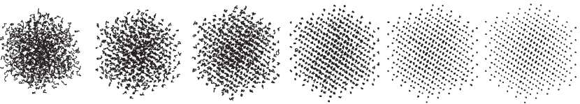
  (a) $\rho=0.6$       (b) $\rho=0.7$       (c) $\rho=0.8$       (d) $\rho=0.9$       (e) $\rho=1.0$        (f) $\rho=1.1$

Figure 2: Atomic Trajectories in Simulation Box. Plot of individual atomic trajectories from an initial condition where atoms are placed on the sites of an FCC lattice and at rest. The trajectory is computed using the numerical and physical parameters indicated in Table 1, with the exception of the # of steps which is set equal to $N_{s}=1000$. At the lower densities the particle trajectories are more diffusive and less localized.

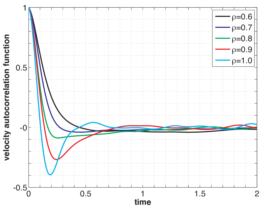
Figure 3: Soft–sphere Velocity Autocorrelation Functions. A reproduction of Figure 5.2 of Rapaport (2004) using Langevin dynamics with heat bath parameter $\gamma=0.01$. The remaining parameters are set equal to those provided in Table 1. The negative correlations at higher densities are consistent with what has been found in the literature Rahman (1964); Alder and Wainwright (1967).

4 Potential Pitfalls in High Dimension & Tricks for Mitigation

For high dimensional systems (think $N>10^{3}$ atoms), calculating the force-field at every step is the main computational cost of MD simulation. These force fields involve: bonded interactions, and non-bonded Lennard-Jones & electrostatic interactions. The calculation of bonded interactions is straightforward to vectorize and scales like $O(N)$. In addition, Lennard-Jones forces rapidly decay with interatomic distance. To a good approximation, every atom interacts only with neighbors within a sufficiently large ball. By using data structures like neighbor lists and cell linked-lists, these interactions can be calculated in $O(N)$ steps, and therefore, the Lennard-Jones interactions can be calculated in $O(N)$ steps Yao et al. (2004). On the other hand, the electrostatic energy between particles decays like $1/r$ where $r$ denotes an interbead distance which leads to long-range interactions between atoms. Unlike Lennard–Jones interaction, this interaction cannot be cutoff without introducing large errors. In this case, one can use sophisticated analysis-based techniques like the fast multipole method to rigorously handle such interactions in $\mathcal{O}(N)$ steps Greengard and Rokhlin (1987); Weinan (2011).

However, the effect of these ‘mathematical tricks’ for fast calculation of the force field can become muted if the time-step requirement for stability or accuracy becomes more severe in high dimension. This can happen in the Metropolis integrator, if the acceptance probability in (Step 2) of Algorithm 3.1 deteriorates in high dimension. The scaling of Metropolis algorithms has been quantified for the random walk Metropolis, hybrid Monte-Carlo, and MALA algorithms Gelman et al. (1997); Roberts and Rosenthal (1998); Beskos et al. (2009, ); Mattingly et al. (2012). Since the acceptance probability is a function of an extensive quantity, the acceptance rate can artificially deteriorate with increasing system size unless the time-step is reduced. Because high acceptance rates are required to maintain dynamic accuracy, the dependence of the time-step on system size limits the application of Metropolized schemes to large-scale systems. Fortunately, this scalability issue can often be resolved by using local rather than global proposal moves because the change in energy induced by a local move is typically an intensive quantity. For molecular dynamics calculations, this approach was pursued in Bou-Rabee and Vanden-Eijnden (2012). Using dynamically consistent local moves (a so-called J-splitting Kang and Dao-Liu (1994)), it was shown that in certain situations a scalable Metropolis integrator can be designed; however, the extent to which this strategy remedies the issue of high rejection rate in high dimension is not clear at this point, and should be tested in applications.

5 Conclusion

This paper provided a step-by-step algorithmic introduction to new analysis-based MD integrators for MD simulation. These algorithms are long-time stable and finite-time accurate for MD simulation. A MATLAB implementation of the algorithm was provided, and used to compute the velocity autocorrelation of a sea of Lennard–Jones particles at various densities between the solid and liquid phases. The paper did not review the theory of Metropolis integrators which is discussed elsewhere Bou-Rabee and Vanden-Eijnden (2010, 2012). We conclude by mentioning two directions for future development.

• The compatibility of the Metropolis integrator with a fast multipole method for handling the electrostatic effects has not been investigated. This loose end is indicated by the question mark appearing towards the right end of the timeline in Figure 1, which points out that an $O(N)$ Metropolis integrator is currently unavailable.

• Another issue is the development of second-order Metropolis integrators for (13) which might permit larger time-steps. The ‘quasi-symplectic’ second–order Langevin integrators introduced in Vanden-Eijnden and Ciccotti (2006) would be a natural starting point for designing proposal moves that would lead to second-order Metropolis integrators.