On the estimation of gravitational wave spectrum from cosmic domain walls
Abstract
We revisit the production of gravitational waves from unstable domain walls analyzing their spectrum by the use of field theoretic lattice simulations with grid size , which is larger than the previous study. We have recognized that there exists an error in the code used in the previous study, and the correction of the error leads to the suppression of the spectrum of gravitational waves at high frequencies. The peak of the spectrum is located at the scale corresponding to the Hubble radius at the time of the decay of domain walls, and its amplitude is consistent with the naive estimation based on the quadrupole formula. Using the numerical results, the magnitude and the peak frequency of gravitational waves at the present time are estimated. It is shown that for some choices of parameters the signal of gravitational waves is strong enough to be probed in the future gravitational wave experiments.
pacs:
98.80.Cq, 04.30.DbI Introduction
Gravitational wave Maggiore (2007) is one of the most promising observational probes of the physics of the early universe. It has been considered that there exist many possibilities to generate observable signatures of gravitational waves in the early universe Maggiore (2000); Binetruy et al. (2012). These include quantum fluctuations during inflation Grishchuk (1975), the first order phase transition Witten (1984), cosmic strings Vilenkin (1981a), non-perturbative decay of the inflaton (preheating) Khlebnikov and Tkachev (1997); Easther and Lim (2006), and so on. It is expected that the observation of such signals of gravitational waves significantly improves our understandings of fundamental physics. These days a number of experimental searches including ground-based Abramovici et al. (1992); Acernese et al. (2008); Willke et al. (2002); Somiya (2012); Sathyaprakash et al. (2012) and space-borne Seto et al. (2001); Amaro-Seoane et al. (2012) observations are running or planned. Accordingly, it is important to understand the nature of sources that are relevant to observations.
In this paper, we study domain walls as a source of primordial gravitational waves. Domain walls are sheet-like objects which are formed in the early universe when a discrete symmetry is spontaneously broken [see e.g. Vilenkin and Shellard (2000)]. It is known that the existence of stable domain walls conflicts with the standard cosmology, since their energy density tends to dominate over the total energy density of the universe Zeldovich et al. (1974). However, it remains a possibility to consider the case where domain walls are unstable, which annihilate at sufficiently early times in order not to affect the standard cosmological history Vilenkin (1981b); Gelmini et al. (1989); Coulson et al. (1996); Larsson et al. (1997). Such unstable but long-lived domain walls would be another source of the stochastic gravitational wave background observed today Gleiser and Roberts (1998); Hiramatsu et al. (2010); Kawasaki and Saikawa (2011).
In the literature, it is discussed that several particle physics models predict the formation of unstable domain walls and the signature of gravitational waves produced from them. For instance, the spontaneous breaking of the discrete R-symmetry in supersymmetric theories would lead to the formation of domain walls Dine et al. (2010), and gravitational waves produced from them can be regarded as a probe of the gravitino mass Takahashi et al. (2008). Domain walls are also formed in the thermal inflationary scenario Moroi and Nakayama (2011), which also predicts signatures relevant to observations. In addition, the production of gravitational waves from domain walls is discussed in the context of the next-to-minimal supersymmetric standard model (NMSSM) in Hamaguchi et al. (2012), the extension of the standard model with right-handed neutrinos in Ishida et al. (2013), and the axion models in Hiramatsu et al. (2011, 2013). Predictions of these models rely on the form of the spectrum of gravitational waves, which necessitates further investigations.
The spectrum of gravitational waves from domain walls is computed by using the numerical simulation of the classical scalar field in Refs. Hiramatsu et al. (2010); Kawasaki and Saikawa (2011). In these previous studies, it was found that the spectrum becomes almost flat extending intermediate frequencies between the scale corresponding to the horizon size at the decay time of domain walls and that corresponding to the width of them. However, the shape of the spectrum and its dependence on some theoretical parameters are not fully understood, due to the lack of the dynamical range of the numerical simulations. In this work, we check the previous results Hiramatsu et al. (2010); Kawasaki and Saikawa (2011) by performing high-resolution simulations with grids. The large dynamical range of the current simulation enables us to investigate the dependence on the parameter controlling the width of domain walls, which was not investigated in the previous studies. Furthermore, in updating the numerical code we recognized that the code used in the previous studies Hiramatsu et al. (2010); Kawasaki and Saikawa (2011) contained an error in the evaluation of the transverse-traceless projection of the stress-energy tensor. In this paper we correct this error and discuss its influence on the numerical results. Correcting the error does not modify the result on the estimation of the overall amplitude of gravitational waves, but the amplitude becomes suppressed at high frequencies with a slope , rather than the flat spectrum observed in the previous results.
The rest of this paper is organized as follows. In Sec. II, we briefly review the evolution of the network of unstable domain walls. After that, in Sec. III we describe the analysis method to calculate the evolution of domain walls and gravitational radiations from them. Results of the numerical study are presented in Sec. IV. In Sec. V, we estimate the amplitude and frequency of gravitational waves observed today by using the numerical results. Finally, we conclude in Sec. VI. Details of the error in the numerical code are described in Appendix A.
II Domain wall network evolution
In this paper, we work in the spatially flat Friedmann-Robertson-Walker (FRW) universe,
where is the scale factor of the universe. Then we consider the model of the real scaler field , whose Lagrangian density is given by
| (1) |
For the scalar potential , we adopt the following double well potential
| (2) |
In the early universe with a finite temperature , the correction term would be added to this potential, and the discrete symmetry () is restored. When the temperature is cooled below the critical value , this symmetry is spontaneously broken to form domain walls.
Once the domain walls are formed, their curvature radius is rapidly homogenized due to the surface tension of them. Eventually they evolve toward the “scaling regime” where the typical length scales of the network of them, such as the curvature radius and the distance between neighboring walls, become comparable to the Hubble radius . In other words, there always exists one (or a few) domain wall(s) inside the horizon in the scaling regime. The appearance of this scaling property is confirmed by various numerical and analytical studies Press et al. (1989); Garagounis and Hindmarsh (2003); Oliveira et al. (2005).
Since the typical size of domain walls is given by the Hubble radius in the scaling regime, the energy density of domain walls evolves as
| (3) |
where is the surface mass density of domain walls. Hence it would be useful to introduce the scaling parameter (or area parameter) Hiramatsu et al. (2012, 2013) given by
| (4) |
We expect that the quantity remains constant during the scaling regime. This property will be checked by numerical simulations in Sec. IV.
In the scaling regime, domain walls frequently interact with each other, changing their configuration or collapsing into the closed walls, to reduce their energy and maintain the scaling property (3). During such a process, a fraction of the energy of domain walls is released as gravitational waves. The magnitude of gravitational waves radiated from them can be estimated by using the quadrupole formula Hiramatsu et al. (2013). With the assumption that the typical time scale of the gravitational radiation is comparable to the Hubble time, the power of gravitational radiation is given by , where is the Newton’s constant, is the quadrupole moment of the domain walls, and is the mass energy of them. Therefore, the energy density of gravitational waves is estimated as
| (5) |
Note that does not depend on the cosmic time . Therefore, we introduce the efficiency parameter Hiramatsu et al. (2013)
| (6) |
which is expected to be constant in the scaling regime. In Sec. IV, we will see that the value of becomes almost constant at late times of the numerical simulations.
The existence of the long-lived domain wall networks is problematic, since the energy density of them () decreases slower than that of matters and radiations. If they are stable, they eventually overclose the universe, which might conflict with the standard cosmological scenario. In order to avoid this problem, they must decay at sufficiently early times. The decay of domain walls can be promoted by introducing a so-called “bias” term in the potential, which explicitly breaks the discrete symmetry. As in the previous studies Hiramatsu et al. (2010); Kawasaki and Saikawa (2011), we use the following term to model this effect
| (7) |
and treat as a free parameter. This term lifts the degenerate vacua and induces the difference in the energy density between them . This difference in the energy density affects on the wall as a volume pressure, . The annihilation of the domain wall networks occurs when this volume pressure becomes comparable to the surface tension of the wall , where is the curvature radius of them. From the condition , we can estimate the decay time of walls as
| (8) |
where we assumed the radiation dominated universe to use .
The magnitude of the parameter is assumed to be sufficiently small such that it breaks the discrete symmetry only approximately. In order that domain walls with infinite size are formed, it must satisfy Hiramatsu et al. (2010). Furthermore, we can obtain the following lower bound on by requiring that domain walls disappear before they overclose the universe,
| (9) |
where is the Planck mass. The possible scenarios with biased domain walls and constraints on are discussed in Refs. Gelmini et al. (1989); Hiramatsu et al. (2010).
Although the formulae (8) and (9) are derived from the bias term of the form (7), other terms which explicitly violate the discrete symmetry (such as ) induce similar effects. If we use the bias term whose form is different from Eq. (7), the numerical coefficients of Eqs. (8) and (9) would be modified, which just affects the estimation of the decay time of domain walls by a factor of .
It should be noted that we perform the simulation without including the explicit symmetry breaking term (7), and do not simulate the collapse of domain walls. Instead, we determine the numerical coefficients such as and , which are defined in the scaling regime, from the results of the simulations. Then, we estimate the present density and frequency of gravitational waves in Sec. V with the assumption that domain walls suddenly disappeared at the time given by Eq. (8). Therefore, the dependence on the parameter appears in the analytic formulae presented in Sec. V through the relation (8).
There are two reasons why we drop the bias term (7) in the present numerical study. Firstly, the inclusion of the bias term leads to a subtlety in the estimation of parameters characterizing the scaling regime. The numerical simulations of domain wall networks with the bias term were performed in Refs. Larsson et al. (1997); Hiramatsu et al. (2010). In these works, it was confirmed that the area of domain walls within the simulation box rapidly falls off in the time scale estimated by Eq. (8). However, in such kind of the simulation, it is difficult to reproduce the scaling regime before the onset of the decay of domain walls due to the limitation of the dynamical range, and the numerical factors such as and are not determined unambiguously. The second reason is that the effect of the bias term might be negligible as long as we are interested in the form of the spectrum relevant to the observations. In Ref. Hiramatsu et al. (2010) it was found that the decay of domain walls leads to make a peak-like feature in the high frequency region of the gravitational wave spectrum, which can be interpreted as the fragmentation of the false vacuum regions into small pieces. As we will see in the following sections, such a feature at the high frequency is irrelevant to the observations, while it is possible to observe the low frequency region comparable to the Hubble parameter at the decay time. With the expectation that the spectrum of interest in observations (i.e. the spectrum at low frequencies) preserves the form produced in the scaling regime, in this work we estimate the spectrum at the present time by extrapolating the result of the numerical simulation obtained in the scaling regime, and ignore the effect of the bias term.
III Simulation techniques
In this section, we describe some technical aspects of the numerical study to calculate the quantities such as the scaling parameter and the spectrum of gravitational waves. We solve the equation of motion of the scalar field in the FRW background on the three dimensional lattice with the periodic boundary condition,
| (10) |
with the potential given by Eq. (2). The spatial derivative is computed by using the fourth order finite difference method, and the time evolution is solved by using the fourth order symplectic integration scheme Yoshida (1990). Note that we are not using the PRS algorithm Press et al. (1989); Sousa and Avelino (2010), in which the equation of motion is modified from Eq. (10) such that the width of domain walls is fixed in the comoving simulation box. This algorithm enables us to improve the dynamical range of the simulation since we do not have to care about the resolution of the width of domain walls [see discussions below Eq. (28)]. However, if we use this algorithm we incorrectly estimate the dynamics at the small scale, which affects the result of the spectrum of gravitational waves. As a check, we performed test simulations by using the modified equation of motion suggested by Press et al. (1989); Sousa and Avelino (2010), and confirmed that the result for the spectrum of gravitational waves becomes different compared with that obtaind from the simulation with the canonical equation of motion (10), even though the result for the scaling parameter (4) is the same in each scheme.
III.1 Initial conditions
The initial field configuration is generated in a similar way to the previous study Kawasaki and Saikawa (2011). In the momentum space, we give the initial value of the scalar field and its time derivative as Gaussian random fields, such that they satisfy the correlation function induced by quantum fluctuation of the massless scalar field:
| (11) |
Since the spectrum of the field diverges at large , we truncate the modes whose wavenumber is higher than a cutoff scale , and treat as the input parameter of the numerical simulation. The large initial field fluctuations at large would affect the result of the numerical simulation since the simulation time is not so long enough for the initial fluctuations to be diluted. A simple way to avoid the contamination from the initial field fluctuations is to use the Gaussian initial condition (11) with a sufficiently small value of , which suppresses the unexpected feature on the gravitational wave spectrum at large . We compared the result of the numerical simulation with varying the value of and confirmed that the dependence on the choice of the initial conditions hardly appears as long as we use the value . Regarding this fact, we use this Gaussian initial condition with in the results shown in this paper.
III.2 Scaling parameter
In each realization of the simulation, we checked the scaling property represented by Eq. (3). This property can be investigated in two ways: One is to compute the area of the surface of domain walls in the simulation box and check the constancy of the scaling parameter defined in Eq. (4). The other is to follow the evolution of the energy density of domain walls , which can be calculated from the data of the scalar field in the simulation box. In this work we carry out both ways to confirm the scaling property of domain walls.
In numerical simulations, the scaling parameter is computed as follows. Let us denote the area of domain walls in the comoving coordinate as , and the volume of the comoving simulation box as . Since the energy of domain walls existing within the simulation box becomes , the energy density is given by
| (12) |
Substituting it into Eq. (4), we obtain
| (13) |
The area of domain walls is computed by the use of the algorithm introduced in Ref. Press et al. (1989). We compare the sign of the scalar field between two neighboring grid points (let us call it as a link), defining the quantity which takes if the sign changes on the link and otherwise. Then, we sum up over all links in the simulation box with multiplying a weighting factor:
| (14) |
where is the area of one grid surface, is the spacing between two neighboring grid points, and are the spatial derivatives of . The weighting factor takes account of the average number of links per area segment. This calculation scheme is used in the other literature to estimate the scaling property of domain walls Press et al. (1989); Oliveira et al. (2005).
To check the scaling law, we also estimate directly without using Eq. (12). Here, the average of the energy density of domain walls in the simulation box is evaluated from the total energy density of the scalar field inside the core of them:
| (15) |
where a term “grids” indicates the summation over all grid points, and is given by
| (16) |
The region of the core of walls is identified as follows. Firstly, we identify the grid points on which the link with is attached, and call them as the “loci of walls”. Then, we increment the grid points within the distance from the loci of walls to evaluate the right-hand-side of Eq. (16), where is the width of domain walls.
III.3 Spectrum of gravitational waves
The spectrum of gravitational waves is computed by using the method developed by Dufaux et al. (2007), which was originally introduced to estimate the gravitational waves produced at preheating after inflation Khlebnikov and Tkachev (1997); Dufaux et al. (2007). This method enables us to compute the spectrum of gravitational waves at a given time as a time integral of the source term constructed from the spatial derivative of the scalar field convoluted with the homogeneous solutions of the equations for metric perturbations.
Here we use the notations of Ref. Hiramatsu et al. (2013) and briefly summarize formulae for the power spectrum of gravitational waves. The spectrum of gravitational waves at the time is given by
| (17) | ||||
| (18) |
where represents the measure of the integration over the direction of , and and are given by
| (19) |
In Eq. (19), we introduced the conformal time defined by , and represents the initial time of the numerical simulation. is the source function defend as follows
| (20) |
is constructed from the transverse traceless (TT) projection of the stress-energy tensor of the scalar field:
| (21) | ||||
| (22) | ||||
| (23) | ||||
| (24) |
where represents the Fourier transform of .
In addition to the estimation of the spectrum of gravitational waves, we also compute the efficiency parameter defined in Eq. (6). Integrating Eq. (17), we obtain the total energy density of gravitational waves:
| (25) |
From Eqs. (6) and (25), the efficiency parameter can be estimated as
| (26) |
It should be noted that the normalization of the spectrum of gravitational waves can be fixed such that it reproduces the value of obtained from numerical simulations when we take the integral of the quantity ) over . However, as we will see in Sec. IV.2, the integration procedure contains a large systematic uncertainty, and it would be practically difficult to fix the normalization of the spectrum by using the integrated quantity such as . Therefore, instead of using to determine the normalization of the spectrum of gravitational waves, we will use the differential amplitude defined as follows
| (27) |
where the subscript “peak” implies that the value is computed at the peak of the spectrum . Since this quantity is defined at the peak wavenumber, we expect that the value of also approaches a constant in the scaling regime. We will check the constancy of and estimate its value in Sec. IV.2.
III.4 Parameters used in the simulations
Let us make a comment on the parameters used in the numerical simulations. In numerical studies we normalize all dimensionful quantities in the unit of . In this unit, denoting the grid size and the box size as and , respectively, we performed simulations for two cases, and . In both cases the time integration is performed with the interval in the conformal time. The time evolution of the scale factor is determined such that it follows the expansion in the radiation dominated universe (). The normalization of the scale factor is taken such that at the initial time of the simulation, and we fix the initial time as . The final time of the simulation is chosen as for simulations with and for those with . Hence the dynamical range of the simulation becomes for and for . Note that the dynamical ranges of the current simulations are much larger than that of the previous studies Hiramatsu et al. (2010); Kawasaki and Saikawa (2011), where we used and .
The other theoretical parameter is the coupling constant in the potential (2), which controls the surface mass density and the width of domain walls. Note that the value of this parameter is constrained from the requirements that the Hubble radius must be shorter than the box size, and that the width of domain walls must be larger than the physical lattice spacing . The scale of the Hubble radius and the width of domain walls divided by the physical lattice spacing are given by
| (28) |
We require that at least the conditions and must be satisfied at the end of the simulation . In the previous studies Hiramatsu et al. (2010); Kawasaki and Saikawa (2011), we fixed the value of with satisfying the above conditions due to the limitation of the dynamical range of the simulation. On the other hand, in the current simulations we can vary the value of and compare the results with different values of . Here, we perform simulations for three choices of the parameter, , , and .
The parameters used in the simulations are summarized in Table LABEL:tab1. For each value of , we execute 10 realizations with and 1 realization with . Before calculating the quantities such as the scaling parameter and the spectrum of gravitational waves, we take an average over 10 realizations for the simulations with . Hence we perform simulations in 6 different sets of parameters as shown in Table LABEL:tab1 [case (a) to (f)]. Note that the requirements described below Eq. (28) are satisfied for every set of parameters. We also note that the dependence on the bias parameter appearing in Eq. (7) is not investigated in the numerical study, since we do not simulate the collapse of domain walls. Effects of the different choice of parameters on the numerical results will be discussed in the next section.
| Case | Grid size () | Box size () | (at ) | (at ) | Realization | |
|---|---|---|---|---|---|---|
| (a) | 80 | 0.03 | 256 | 2.61 | 10 | |
| (b) | 80 | 0.01 | 256 | 4.53 | 10 | |
| (c) | 80 | 0.003 | 256 | 8.26 | 10 | |
| (d) | 120 | 0.03 | 512 | 2.32 | 1 | |
| (e) | 120 | 0.01 | 512 | 4.02 | 1 | |
| (f) | 120 | 0.003 | 512 | 7.34 | 1 |
IV Results
IV.1 Scaling properties
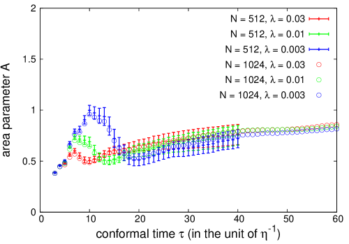
Figure 1 shows the evolution of the area parameter defined in Eq. (4). We see that the value of becomes almost constant at late times, which implies that the network of domain walls obeys the scaling law at the late time of the simulations. We note that the value of does not depend on the choice of . Approaching to the constant value is observed more obviously in the simulations with than those with , except for the fact that the value of slightly increases around the final time of the simulations. It is presumed that this deviation from the constancy is caused by the finiteness of the simulation box, since the Hubble radius becomes comparable to the box size at the final time of the simulations. This effect would be removed if we performed the simulation with a larger box size.
As shown in the plot for the simulations with , there is a statistical uncertainty of due to the different realizations. Including this uncertainty, we estimate the value of in the scaling regime as
| (29) |
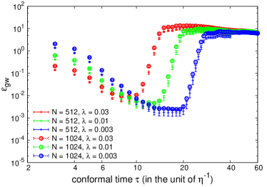
We also plot the time evolution of the energy density of domain walls in Fig. 2. We confirm that evolves along to the scaling law at late times. The magnitude of the energy density scales as , which coincides with the relations and . We also observe that the onset of scaling (or the formation time of the horizon-sized walls) depends on . This formation time scale might be estimated from the condition that the width of walls becomes comparable (or shorter than) the Hubble radius . This condition gives , as shown in Fig. 2.
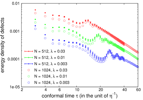
We note that the disagreement between the results for and those for at the early times of the simulations in Fig. 2 is caused by the fact that we cannot correctly determine the core region of domain walls before they enter into the scaling regime. At the initial time, the scalar field distributes according to the initial condition described in Sec. III.1, and it varies with an interval . Since we identify the loci of walls as the place where the scalar field changes its sign, as long as the lattice spacing is shorter than , in Eq. (15) does not change so much for fixed value of at the initial time (though it depends on the simulation box size), while in the left-hand side of Eq. (15) is suppressed by the factor . This is the reason why the result of for is smaller than that for at the initial stage of the simulation. It should be emphasized that this difference at the initial stage due to the numerical artifacts in the initial conditions is a matter of minor importance for our purpose, since we are interested in the evolution of domain walls during the scaling regime. Indeed, from Fig. 2 we see that the difference of the results between simulations with and is not prominent after walls enter into the scaling regime.
IV.2 Gravitational waves
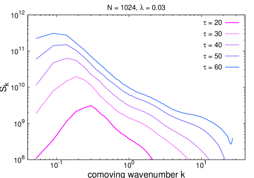
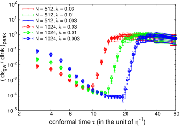
Next, let us show the results for the spectrum of gravitational waves. In Fig. 3, we plot the time evolution of the spectrum obtained form the simulation with and . This result indicates that the spectrum peaks at small while the amplitude is suppressed at large . The form of shown in Fig. 3 differs from the previous result Hiramatsu et al. (2010); Kawasaki and Saikawa (2011) in which the spectrum becomes rather flat in the intermediate scale. As we describe in Appendix A, this discrepancy is due to the fatal error in numerical codes used in the previous studies.
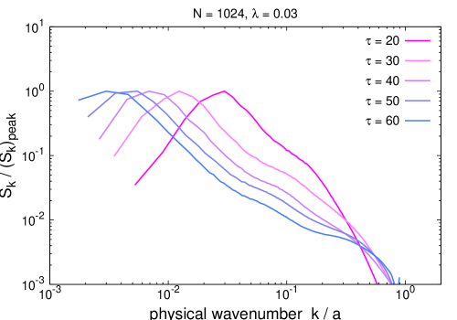
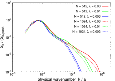
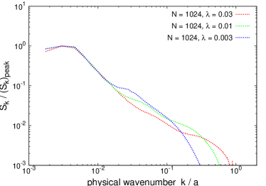
We also plot the evolution of the spectrum with taking the horizontal axis as the physical wavenumber in Fig. 4. This figure indicates that the peak is located at the horizon scale, which shifts with time as . On the other hand, we also observe that the spectrum always falls off at a large wavenumber , whose location does not seem to depend on time. We deduce that this falloff corresponds to the microscopic scale determined by the width of domain walls (). This speculation can be checked in part when we compare the results for different values of , as shown in Fig. 5. We see that the falloff of the spectrum occurs at higher momentum region for the result with larger value of . This result is consistent with the above speculation that the spectrum extends up to the scale . On the other hand, the peak location scarcely depends on the value of , from which we confirm that the peak is determined by the Hubble parameter. The slope of the spectrum in the intermediate scale between the Hubble radius and the width of walls is not determined straightforwardly, but from the results with the larger dynamical range [Fig. 5 (b)] we observe that decreases as at large wavenumbers.
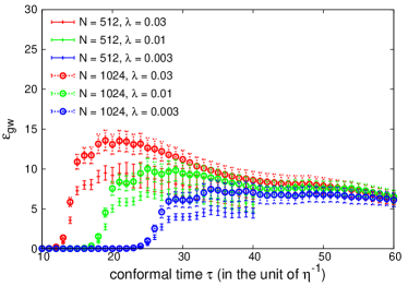
Figures 6 (a) and (b) show the evolution of the efficiency parameter defined in Eq. (26). From these figures we see that the magnitude of rapidly grows at the time of the formation of domain walls, and it remains almost constant value of at late times. It should be noted that there are various uncertainties on the determination of the value of . First of all, there are two statistical errors shown as error bars in figures. One is the variation for each realization of the simulation. This statistical error is not included in the results of the simulations with , since we performed one realization only. The other kind of error arises when we evaluate the integration over the direction of to obtain the spectrum . In numerical analysis, we compute in Eq. (18) by averaging all data defined on the shell with in -space. We estimate the statistical error as a standard deviation arising in this averaging procedure. In addition to these statistical errors, there is a systematic error, which appears in the difference in the results between the simulation with and that with [see Figs. 6 (a) and (b)]. This difference occurs due to the poor resolution of the peak of the spectrum (i.e. the small number of bins at small ) when we integrate over to obtain by using Eq. (26). Since there is a few data points in small and the peak of is located there, we are apt to underestimate the total amplitude if the grid number is small.
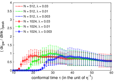
To check that the systematic error described above arises due to the integration over with discretized grids, we also compute the differential amplitude given by Eq. (27). Since this quantity is just determined by the peak amplitude, we expect that its value is unaffected by the uncertainty in the discretization scheme. Figures 6 (c) and (d) show the evolution of , from which we confirm that the results do not depend on the choice of , and that it takes almost constant value in the scaling regime. However, we also see that the statistical error becomes large () in these plots.
As was noted in Sec. III.3, we can fix the normalization of the spectrum by using the value determined from numerical simulations. From the average of six data points plotted at in Fig. 6 (c), we obtain
| (30) |
where we took a conservative error (% of the mean value), regarding the large statistical uncertainties. We will use this value to estimate the present density of gravitational waves in Sec. V.
V Present density of gravitational waves
In this section, we estimate the amplitude and frequency of gravitational waves observed today by using the numerical results described in the previous section. The amplitude can be estimated from the fact that the energy density of gravitational waves remains almost constant during the scaling regime
| (31) |
Alternatively, we can estimate the amplitude at the peak of the spectrum in terms of the quantity defined in Eq. (27):
| (32) |
Assuming that the gravitational radiation terminates at the decay time of domain walls (), and that the decay completes in the radiation dominated era, we estimate the fraction between the energy density of gravitational waves and the total energy density of the universe at the decay time as
| (33) |
where
| (34) |
is the Hubble parameter at . If the production of gravitational waves completes in the radiation dominated era, the present density of gravitational wavs is estimated as
| (35) |
where represents the present time, is the reduced Hubble parameter (), is the density parameter of radiations at the present time, and and are the relativistic degrees of freedom at the present time and at , respectively. Combining Eqs. (33)-(35), we obtain
| (36) | ||||
| (37) |
where we used the mean values of and obtained from the numerical results, and , in the second line.
On the other hand, the peak frequency of the gravitational waves is determined by the Hubble parameter at the decay time. Let us denote this frequency as . We can estimate the present value of the frequency by multiplying the scale by the redshift factor ,
| (38) |
Using the relation
we obtain
| (39) |
In Sec. IV, we observed that the spectrum extends up to the wavenumber , which corresponds to the width of domain walls. The frequency determined by this length scale can also be estimated as
| (40) |
Though the peak amplitude and frequency can be determined by the use of Eqs. (37) and (39), the estimation of the amplitude at high frequencies is subtle. In the previous studies Hiramatsu et al. (2010); Kawasaki and Saikawa (2011), we extrapolated the numerical results, in which the slope of the spectrum becomes almost flat in the intermediate frequency range . However, the updated spectrum obtained in Sec. IV indicates that the amplitude at is suppressed compared with that at . It is not so straightforward to estimate the degree of suppression, but the results of the current simulations indicate the behavior in the intermediate frequencies .
We note that the spectrum at low frequencies can be deduced from the requirement of causality Caprini et al. (2009). To discuss this point, let us write the spectrum of gravitational waves at the production time in the radiation dominated era as Kawasaki and Saikawa (2011)
| (41) |
where is some onset of the production of gravitational waves. In the above equation, represents the unequal time correlator of the anisotropic stress tensor
| (42) | ||||
| (43) |
where represents an ensemble average, and is the pressure of the background fluids ( in the radiation dominated universe). Note that can be written in terms of the Fourier transform of the correlation function in the real space
| (44) | ||||
| (45) |
From causality it is required that for , where is the correlation length. This fact implies that the integration over in Eq. (44) is truncated at . Therefore, if we consider the mode satisfying , the integrand in Eq. (44) can be expanded as a power series of . As a result, approaches a value which does not depend on in the limit , if the leading contribution of the power series expansion does not vanish. In this case, the slope of the spectrum is purely determined by the factor in Eq. (41) for small . This behavior can be checked in part, by computing the equal time correlation function directly from the results of numerical simulations Kawasaki and Saikawa (2011). We compute for the sets of simulations described in Sec. IV and observed that hardly depends on for .
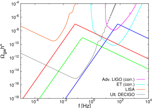
Figure 7 shows schematics for the spectrum of gravitational waves produced by domain walls in comparison with sensitivities of planned detectors such as (Advanced) LIGO Abramovici et al. (1992), ET Sathyaprakash et al. (2012), LISA Amaro-Seoane et al. (2012), and Ultimate DECIGO Seto et al. (2001). For LISA and DECIGO, we estimated the sensitivity curve in terms of the formula for the minimum detectable amplitude of in the single detector Maggiore (2007, 2000):
which reduces to
| (46) |
where is the noise spectral density, is the signal-to-noise ratio for a confident detection, and is the angular efficiency factor of the detector. Here we fix the value of as , which corresponds to the interferometer with perpendicular arms Maggiore (2007, 2000), and use a reference value . On the other hand, for LIGO and ET, we assume to take the correlation between two detectors, which improves the sensitivity by several orders of magnitude Maggiore (2007, 2000):
| (47) |
where is the total observation time, and is the frequency resolution of the detectors. In the plots shown in Fig. 7, we choose and . We note that Eq. (47) does not take account of the separation between two detectors. In the realistic cases, the sensitivity would be suppressed at high frequencies due to the fact that two detectors are placed at different location and have a different angular sensitivity. Here we do not include this reduction factor for the sake of a rough comparison.
In Fig. 7, we plot the peak amplitude and frequency obtained from Eqs. (37) and (39) for selected values of and satisfying the condition (9). Note that the peak amplitude and frequency are controlled by three theoretical parameters (, , and ) such that and . The speculative estimates for the slope of the spectrum ( for and for ) are also shown as the broken lines. As shown in this figure, if the peak frequency corresponding to the horizon scale at the decay time of domain walls lies within the frequency band in which the planned detectors are sensitive, the signatures of gravitational waves can be probed in future experimental studies.
VI Conclusion
In this paper, we have calculated the spectrum of gravitational waves produced by domain walls based on the lattice simulations with improved dynamical ranges. The large dynamical range enables us to survey the dependence on the theoretical parameter , which controls the energy and width of domain walls. It is found that the spectrum has a peak at the wavenumber corresponding to the horizon size, regardless of the value of , and that it falls off at a large wavenumber. The location of the falloff varies with the value of , which indicates that this scale corresponds to the width of domain walls. The slope of the spectrum in the intermediate scales behaves like . This result is different from the previous one Kawasaki and Saikawa (2011), where the spectrum becomes almost flat, but this difference is caused by the error in the numerical code used in the previous studies.
From the results of the numerical simulations, the scaling parameter and the differentiation of the efficiency parameter at the peak of the spectrum are determined as Eqs. (29) and (30). Using the values of and obtained from the simulations, we estimate the amplitude of gravitational waves observed today as Eq. (37). The estimation of involves large statistical uncertainties, which is caused by the variation of the results for different realizations and the uncertainty in the integration over the direction of in -space. As a result, the estimation for the present density of gravitational waves (37) contains the uncertainty as a factor of . The present value of the peak frequency is also estimated as Eq. (39). If the scale of the symmetry breaking is sufficiently high and domain walls exist for a long time , there exists a parameter region where the signature of gravitational waves can be probed in the future gravitational wave interferometers.
Acknowledgements.
We thank B. S. Sathyaprakash for notifying about the ET sensitivity curve. Numerical computation in this work was carried out at the Yukawa Institute Computer Facility. M. K. is supported by Grant-in-Aid for Scientific research from the Ministry of Education, Science, Sports, and Culture (MEXT), Japan, No. 25400248 and No. 21111006 and also by World Premier International Research Center Initiative (WPI Initiative), MEXT, Japan. K. S. is supported by the Japan Society for the Promotion of Science (JSPS) through research fellowships. T. H. is supported by JSPS Grant-in-Aid for Young Scientists (B) No. 23740186, and also by MEXT HPCI Strategic Program.Appendix A The coding error
The numerical code used in this paper is developed based on that used in Refs. Hiramatsu et al. (2012, 2013). In this code, we modify some schemes from the old code used in Hiramatsu et al. (2010); Kawasaki and Saikawa (2011), improving its operation speed. However, we found that the old code contains an error in evaluating the TT projection of the stress-energy tensor of the scalar field, which leads to the wrong estimation for the gravitational wave spectrum.
The error is just caused by a technical reason. We use the discrete spatial coordinate on the lattice, (ix, iy, iz), where the indices ix, iy, iz are integers taking a value from 0 to N-1, and the scalar field defined on the lattice is stored to an 1D array, f[idx] as
| (48) |
Also for the each element of stress-energy tensor , we store its data to another 1D array, T11[idk], T12[idk], …, but we incorrectly assigned them in the old code as
| (49) |
when we evaluate the TT projection defined in Eq. (21). Clearly, idk should be calculated in the same way as (48). As a result, this mismatch leads to a wrong result, since this treatment corresponds to interchanging and in evaluating Eq. (21).
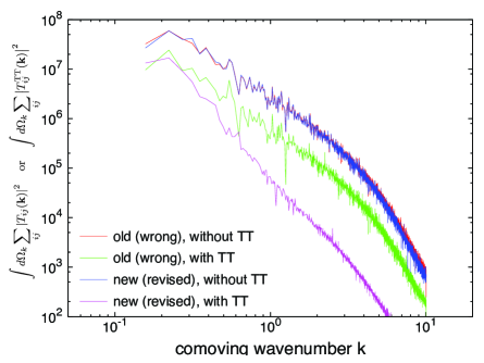
In Fig. 8, we plot the comparison between the results of the old code used in Hiramatsu et al. (2010); Kawasaki and Saikawa (2011) and new code used in this paper. Here, we compute the power of the stress-energy tensor
| (50) |
and its TT projection
| (51) |
Note that the difference does not appear when we compute the power without TT projection (50), since it depends only on . The effect of the wrong assignment (49) arises when we compute the power with TT projection (51), since it depends not only on , but also on the direction . Accordingly, the old code incorrectly estimates the spectrum of gravitational waves. As shown in Fig. 8, for the stress-energy tensor of domain walls, the old code overestimates the power at large wavenumbers, which leads to the almost flat spectrum observed in the previous numerical studies Hiramatsu et al. (2010); Kawasaki and Saikawa (2011).
References
- Maggiore (2007) M. Maggiore, Gravitational Waves. Vol. 1: Theory and Experiments (Oxford University Press, 2007).
- Maggiore (2000) M. Maggiore, Phys.Rept. 331, 283 (2000), eprint gr-qc/9909001.
- Binetruy et al. (2012) P. Binetruy, A. Bohe, C. Caprini, and J.-F. Dufaux, JCAP 1206, 027 (2012), eprint 1201.0983.
- Grishchuk (1975) L. Grishchuk, Sov.Phys.JETP 40, 409 (1975); B. Allen, Phys.Rev. D37, 2078 (1988); V. Sahni, Phys.Rev. D42, 453 (1990).
- Witten (1984) E. Witten, Phys.Rev. D30, 272 (1984); M. Kamionkowski, A. Kosowsky, and M. S. Turner, Phys.Rev. D49, 2837 (1994), eprint astro-ph/9310044.
- Vilenkin (1981a) A. Vilenkin, Phys.Lett. B107, 47 (1981a); F. S. Accetta and L. M. Krauss, Nucl.Phys. B319, 747 (1989); R. Caldwell and B. Allen, Phys.Rev. D45, 3447 (1992).
- Khlebnikov and Tkachev (1997) S. Khlebnikov and I. Tkachev, Phys.Rev. D56, 653 (1997), eprint hep-ph/9701423; J. Garcia-Bellido, D. G. Figueroa, and A. Sastre, Phys.Rev. D77, 043517 (2008), eprint 0707.0839; J.-F. Dufaux, G. Felder, L. Kofman, and O. Navros, JCAP 0903, 001 (2009), eprint 0812.2917; M. Kawasaki, K. Saikawa, and N. Takeda, Phys.Rev. D87, 103521 (2013), eprint 1208.4160.
- Easther and Lim (2006) R. Easther and E. A. Lim, JCAP 0604, 010 (2006), eprint astro-ph/0601617.
- Abramovici et al. (1992) A. Abramovici, W. E. Althouse, R. W. Drever, Y. Gursel, S. Kawamura, et al., Science 256, 325 (1992).
- Acernese et al. (2008) F. Acernese, M. Alshourbagy, P. Amico, F. Antonucci, S. Aoudia, et al., Class.Quant.Grav. 25, 184001 (2008).
- Willke et al. (2002) B. Willke, P. Aufmuth, C. Aulbert, S. Babak, R. Balasubramanian, et al., Class.Quant.Grav. 19, 1377 (2002).
- Somiya (2012) K. Somiya (KAGRA Collaboration), Class.Quant.Grav. 29, 124007 (2012), eprint 1111.7185.
- Sathyaprakash et al. (2012) B. Sathyaprakash, M. Abernathy, F. Acernese, P. Ajith, B. Allen, et al., Class.Quant.Grav. 29, 124013 (2012), eprint 1206.0331.
- Seto et al. (2001) N. Seto, S. Kawamura, and T. Nakamura, Phys.Rev.Lett. 87, 221103 (2001), eprint astro-ph/0108011; S. Kawamura, T. Nakamura, M. Ando, N. Seto, K. Tsubono, et al., Class.Quant.Grav. 23, S125 (2006).
- Amaro-Seoane et al. (2012) P. Amaro-Seoane, S. Aoudia, S. Babak, P. Binetruy, E. Berti, et al., GW Notes 6, 4-110 (2013), eprint 1201.3621.
- Vilenkin and Shellard (2000) A. Vilenkin and E. P. S. Shellard, Cosmic Strings and Other Topological Defects (Cambridge University Press, 2000).
- Zeldovich et al. (1974) Y. Zeldovich, I. Y. Kobzarev, and L. Okun, Zh.Eksp.Teor.Fiz. 67, 3 (1974).
- Vilenkin (1981b) A. Vilenkin, Phys.Rev. D23, 852 (1981b).
- Gelmini et al. (1989) G. B. Gelmini, M. Gleiser, and E. W. Kolb, Phys.Rev. D39, 1558 (1989).
- Coulson et al. (1996) D. Coulson, Z. Lalak, and B. A. Ovrut, Phys.Rev. D53, 4237 (1996).
- Larsson et al. (1997) S. E. Larsson, S. Sarkar, and P. L. White, Phys.Rev. D55, 5129 (1997), eprint hep-ph/9608319.
- Gleiser and Roberts (1998) M. Gleiser and R. Roberts, Phys.Rev.Lett. 81, 5497 (1998), eprint astro-ph/9807260.
- Hiramatsu et al. (2010) T. Hiramatsu, M. Kawasaki, and K. Saikawa, JCAP 1005, 032 (2010), eprint 1002.1555.
- Kawasaki and Saikawa (2011) M. Kawasaki and K. Saikawa, JCAP 1109, 008 (2011), eprint 1102.5628.
- Dine et al. (2010) M. Dine, F. Takahashi, and T. T. Yanagida, JHEP 1007, 003 (2010), eprint 1005.3613.
- Takahashi et al. (2008) F. Takahashi, T. Yanagida, and K. Yonekura, Phys.Lett. B664, 194 (2008), eprint 0802.4335.
- Moroi and Nakayama (2011) T. Moroi and K. Nakayama, Phys.Lett. B703, 160 (2011), eprint 1105.6216.
- Hamaguchi et al. (2012) K. Hamaguchi, K. Nakayama, and N. Yokozaki, Phys.Lett. B708, 100 (2012), eprint 1107.4760.
- Ishida et al. (2013) H. Ishida, K. S. Jeong, and F. Takahashi (2013), eprint 1309.3069.
- Hiramatsu et al. (2011) T. Hiramatsu, M. Kawasaki, and K. Saikawa, JCAP 1108, 030 (2011), eprint 1012.4558.
- Hiramatsu et al. (2013) T. Hiramatsu, M. Kawasaki, K. Saikawa, and T. Sekiguchi, JCAP 1301, 001 (2013), eprint 1207.3166.
- Press et al. (1989) W. H. Press, B. S. Ryden, and D. N. Spergel, Astrophys.J. 347, 590 (1989).
- Garagounis and Hindmarsh (2003) T. Garagounis and M. Hindmarsh, Phys.Rev. D68, 103506 (2003), eprint hep-ph/0212359; A. Leite and C. Martins, Phys.Rev. D84, 103523 (2011), eprint 1110.3486; A. Leite, C. Martins, and E. Shellard, Phys.Lett. B718, 740 (2013), eprint 1206.6043; M. Hindmarsh, Phys.Rev.Lett. 77, 4495 (1996), eprint hep-ph/9605332; M. Hindmarsh, Phys.Rev. D68, 043510 (2003), eprint hep-ph/0207267; P. Avelino, C. Martins, and J. Oliveira, Phys.Rev. D72, 083506 (2005), eprint hep-ph/0507272.
- Oliveira et al. (2005) J. Oliveira, C. Martins, and P. Avelino, Phys.Rev. D71, 083509 (2005), eprint hep-ph/0410356.
- Hiramatsu et al. (2012) T. Hiramatsu, M. Kawasaki, K. Saikawa, and T. Sekiguchi, Phys. Rev. D85, 105020 (2012), eprint 1202.5851.
- Yoshida (1990) H. Yoshida, Phys.Lett. A150, 262 (1990).
- Sousa and Avelino (2010) L. Sousa and P. Avelino, Phys.Rev. D81, 087305 (2010), eprint 1101.3350.
- Dufaux et al. (2007) J. F. Dufaux, A. Bergman, G. N. Felder, L. Kofman, and J.-P. Uzan, Phys.Rev. D76, 123517 (2007), eprint 0707.0875.
- Caprini et al. (2009) C. Caprini, R. Durrer, T. Konstandin, and G. Servant, Phys.Rev. D79, 083519 (2009), eprint 0901.1661.
- (40) URL https://dcc.ligo.org/LIGO-T0900288/public.
- (41) URL https://workarea.et-gw.eu/et/WG4-Astrophysics/base-sensitivity.
- (42) URL http://www.srl.caltech.edu/%7Eshane/sensitivity/index.html.
- Alabidi et al. (2012) L. Alabidi, K. Kohri, M. Sasaki, and Y. Sendouda, JCAP 1209, 017 (2012), eprint 1203.4663.