Long-Term Evolution of Decaying MHD Turbulence in the Multiphase ISM

Abstract

Supersonic turbulence in the interstellar medium (ISM) is believed to decay rapidly within a flow crossing time irrespective of the degree of magnetization. However, this general consensus of decaying magnetohydrodynamic (MHD) turbulence relies on local isothermal simulations, which are unable to take into account the roles of global structures of magnetic fields and the ISM. Utilizing three-dimensional MHD simulations including interstellar cooling and heating, we investigate decaying MHD turbulence within cold neutral medium sheets embedded in warm neutral medium. Early evolution of turbulent kinetic energy is consistent with previous results for decaying compressible MHD turbulence characterized by rapid energy decay with a power-law form of $E\propto t^{-1}$ and by short decay time compared to a flow crossing time. If initial magnetic fields are strong and perpendicular to the sheet, however, long-term evolution of the kinetic energy shows that a significant amount of turbulent energy ($\sim 0.2E_{0}$) still remains even after ten flow crossing times for models with periodic boundary conditions. The decay rate is also greatly reduced as the field strength increases for such initial and boundary conditions, but not if the boundary conditions are that for a completely isolated sheet. We analyze velocity power spectra of the remaining turbulence to show that in-plane, incompressible motions parallel to the sheet dominate at later times.

1 Introduction

Supersonic turbulence is ubiquitous in the interstellar medium (ISM) and is a key ingredient of star formation processes (see Elmegreen & Scalo 2004; Mac Low & Klessen 2004; McKee & Ostriker 2007 for recent reviews). The characteristics and properties of turbulence have long been studied since the pioneering study for incompressible, hydrodynamic turbulence by Kolmogorov (1941), which is applicable mostly to terrestrial flows. For incompressible turbulence, turbulent energy is transferred from larger to smaller scales via eddy cascading all the way down to the dissipation scale, where viscosity is effective. Turbulence in the ISM, however, is expected to depart largely from this classical picture mostly due to its compressibility with supersonic Mach number and non-negligible degree of magnetization. A general theory of incompressible magnetohydrodynamic (MHD) turbulence has been developed by Goldreich & Sridhar (1995) and tested by numerical simulations for both incompressible and compressible gas flows (e.g., Cho & Vishniac 2000; Maron & Goldreich 2001; Lithwick & Goldreich 2001; Cho & Lazarian 2003; Vestuto et al. 2003). Similar energy cascading processes occur in MHD turbulence as well, while the eddies are elongated along the direction of the magnetic field.

The time evolution of turbulent energy is expected to follow a power-law form of $E\propto t^{-\eta}$. The exponent $\eta$ of incompressible hydrodynamic turbulence has been analytically suggested to be $10/7$ from Kolmogorov theory (Kolmogorov, 1941) and experimentally measured to be in a range from $1.2$ to $2$ (Smith et al., 1993). Since supersonic gas flows naturally induce shock waves, that provide additional energy dissipation, turbulent energy is expected to be dissipated away rapidly in less than than lifetime of a molecular cloud in the absence of driving. This theoretical expectation contradicts with universally observed suprathermal linewidths within molecular clouds (e.g., Larson 1981). Magnetic fields have then come into the spotlight to resolve this contradiction. Arons & Max (1975) have suggested non-dissipative linear Alfvén waves as sub-Alfvénic turbulence to explain the observed turbulence without the need for external energy driving (see also Zweibel & Josafatsson 1983; Elmegreen 1985).

Recently, numerical simulations allowed to explore the nonlinear evolution of supersonic MHD turbulence and revealed that the previous belief of long-lived sub-Alfvénic turbulence is incorrect. Gammie & Ostriker (1996) have shown that kinetic energy dissipates quickly in one-dimensional MHD simulations of isothermal compressible decaying turbulence. This work has been extended to three-dimensional local periodic-box simulations by several authors (e.g., Mac Low et al. 1998; Stone et al. 1998; Padoan & Nordlund 1999). The results from simulations for compressible MHD turbulence have converged to a rapid decay of turbulence in the ISM, as $E\propto t^{-1}$, regardless of magnetic field strengths. If the energy transfer to larger scales through the inverse cascade is prevented by energy injection on the scale of the system, Cho & Lazarian (2003) have suggested $\eta$ would become closer to 2. Supersonic turbulence in molecular cloud conditions loses half of the initial energy within a flow crossing time (Ostriker et al., 2001), usually discuss comparable to a free-fall time of the cloud. Based on these numerical studies, the universal supersonic turbulence observed in clouds is now believed to arise from inexhaustible energy input mechanisms, e.g., stellar feedback, gas-dynamical instabilities, galactic rotation, and so on (see Mac Low & Klessen 2004; Elmegreen & Scalo 2004 and references therein).

Although a general consensus of rapidly decaying compressible MHD turbulence has been achieved during the last two decades, the conclusion relies heavily on the results of local isothermal simulations (see also local models for the multiphase ISM; Kritsuk & Norman 2002, 2004). Since these models represent a local patch of a homogeneous medium embedded within a larger cloud, it is not directly applicable to turbulence in the diffuse multiphase ISM. Thermal processes in the ISM naturally induce an inhomogeneity, giving rise to two distinct atomic phases, a cold neutral medium (CNM) and a warm neutral medium (WNM), whose density and temperature differ by about two orders of magnitude (Field et al., 1969; Wolfire et al., 1995). High-resolution 21 cm absorption line observations using the Arecibo telescope have shown that the CNM is generally observed within sheets rather than isotropic clouds (Heiles & Troland, 2003). These CNM sheets have magnetic fields that dominate the thermal pressure of the ISM, with a median strength of $6\;\mu{\rm G}$ (Heiles & Troland, 2005; Crutcher, 2012), while the orientation of the magnetic fields to the sheet is somewhat uncertain. Such commonly observed sheet-like structures of the CNM with strong magnetic fields threading both CNM and WNM suggest that idealized local isothermal models have clear limitations in application to turbulence of the diffuse multiphase ISM. The global structures of the ISM and magnetic fields should be taken into account to study ISM turbulence properly.

Kudoh & Basu (2003, 2006) have considered a stratified molecular cloud using a Lagrangian fluid description for the temperature to model a cold cloud within a hot medium. Their 1.5 dimensional simulations show lower dissipation rates than local isothermal simulations, but it is unclear whether this results from a lack of dimensionality (Mac Low et al., 1998; Ostriker et al., 1999) or the global structure they considered. Using two-dimensional simulations of thin sheets with the external magnetic field calculated as a potential field, Basu & Dapp (2010) have shown that global magnetic tension driven modes produce long-lasting turbulence in the flux-freezing limit, in contrast to previous local models. Without a thin-disk approximation, however, three-dimensional stratified cloud models with Lagrangian fluid elements have reported that energy dissipation occurs differently from Basu & Dapp (2010), but about 10% of the initial kinetic energy remains at the final stage (Kudoh & Basu, 2011).

Motivated by limitations of local isothermal simulations and recent simulations for thin sheets, we investigate the long-term evolution of decaying turbulence. We utilize full three-dimensional simulations with interstellar cooling and heating in order to understand turbulence within the diffuse multiphase ISM. Our numerical models provide alternative perspectives on decaying turbulence within CNM sheets, including the effect of magnetic fields anchored in the ambient WNM as well as non-isothermality and field orientations. This paper is organized as follows. In Section 2, we describe numerical methods and initial model setups. In Section 3.1, we present our main results using temporal evolution of turbulent kinetic energy for models with different magnetic field strengths and orientations. In Section 3.2, we analyze turbulence characteristics in detail, especially strong field models. In Section 4, we discuss our model setup and outcomes in comparison with observations, and Section 5 summarizes our main results.

2 Numerical Methods & Models

In order to investigate the decaying MHD turbulence in the multiphase ISM, we solve a set of ideal MHD equations with cooling, heating, and thermal conduction:

$$\frac{\partial{\rho}}{\partial{t}}+\nabla\cdot\left({\rho\mathbf{v}}\right)=0,$$ (1)

$$\frac{\partial{\rho\mathbf{v}}}{\partial{t}}+\nabla\cdot\left[{\rho\mathbf{v}\mathbf{v}-\frac{\mathbf{B}\mathbf{B}}{4\pi}+\left({P+\frac{B^{2}}{8\pi}}\right)\mathbf{I}}\right]=0,$$ (2)

$$\frac{\partial{E}}{\partial{t}}+\nabla\cdot\left[{\left({E+P+\frac{B^{2}}{8\pi}}\right)\mathbf{v}-\frac{\mathbf{B}}{4\pi}(\mathbf{B}\cdot\mathbf{v})-\mathcal{K}\nabla T}\right]=-\rho\mathcal{L},$$ (3)

$$\frac{\partial{\mathbf{B}}}{\partial{t}}-\nabla\times\left({\mathbf{v}\times\mathbf{B}}\right)=0,$$ (4)

$$\nabla\cdot\mathbf{B}=0,$$ (5)

where $\rho$, $\mathbf{v}$, P, and $\mathbf{B}$ are the total gas mass density, velocity vector, gas thermal pressure, and magnetic field, respectively, as usual. $E$ is the total energy density

$$E=\frac{P}{\gamma-1}+\frac{\rho v^{2}}{2}+\frac{B^{2}}{8\pi},$$ (6)

where $v^{2}=\mathbf{v}\cdot\mathbf{v}$ and $B^{2}=\mathbf{B}\cdot\mathbf{B}$. We adopt the ideal gas law $P=(\gamma-1)e$ with $\gamma=5/3$, where $e$ is the internal energy density. The thermal pressure is $P=1.1nk_{\rm B}T$ for 10% of Helium abundance. Here $n$ is the number density of hydrogen, and hence $\rho=1.4\;m_{\rm H}n$. The thermal conductivity is $\mathcal{K}=10^{5}{\rm\;erg\;s^{-1}\;cm^{-1}\;K^{-1}}$. The source term in the energy equation (Eq. (3)) is the net volumetric cooling given by $\rho\mathcal{L}\equiv n[n\Lambda(T)-\Gamma]$. Following Koyama & Inutsuka (2002), we adopt the simple fitting formula for dominant interstellar cooling, mainly due to [C II], [O I] fine structure and Ly$\alpha$ recombination lines, and the constant heating rate due to the photoelectric effect on grains by FUV photons (Kim et al. 2008 for a typo corrected version):

$$\Lambda(T)=2\times 10^{-19}\exp\left(\frac{-1.184\times 10^{5}}{T+1000}\right)+2.8\times 10^{-28}\sqrt{T}\exp\left(\frac{-92}{T}\right){\rm\;erg}\;{\rm cm}^{3}\;{\rm s^{-1}},$$ (7)

$$\Gamma=2\times 10^{-26}\;{\rm erg}\;{\rm s}^{-1}.$$ (8)

We solve the governing equations using the Athena code that employs the high order Godunov method (Stone et al., 2008; Stone & Gardiner, 2009). Among the various techniques provided by the Athena code to solve the MHD equations, we adopt van Leer integrator (Stone & Gardiner, 2009) with Roe’s Riemann solver and second-order spatial reconstruction scheme. Athena satisfies the divergence-free condition within machine precision via the constrained transport algorithm (Evans & Hawley, 1988). For the cooling source term, we solve it separately using a fully implicit method with a Newton-Raphson iteration (Piontek & Ostriker, 2004; Kim et al., 2008) and update temperature before entering the integrator steps for conservation equations. To ensure the code stability, we reduce the time step until the temperature change is smaller than 50% of the previous temperature. An isotropic thermal conduction is solved explicitly as well.

For an initial state, we assume a thin CNM sheet in a thermal pressure equilibrium with the surrounding WNM. So we first solve thermal equilibrium equation, $\Gamma=n\Lambda(T)$, for a given equilibrium pressure $P_{0}$ to find the density and temperature of the CNM and WNM, $(n_{c},T_{c})$ and $(n_{w},T_{w})$, respectively. For our fiducial parameter of initial thermal pressure, $P_{0}/k_{\rm B}=3000\;{\rm cm}^{-3}\,{\rm K}$ (Wolfire et al., 2003; Jenkins & Tripp, 2011), the equilibrium density and temperature are $(48\;{\rm cm}^{-3},57\;{\rm K})$ and $(0.4\;{\rm cm}^{-3},6500\;{\rm K})$ for the CNM and WNM, respectively. We then assign a uniform CNM for $|z|<\Delta_{c}/2$, where $\Delta_{c}=2\;{\rm pc}$ is the thickness of the CNM sheet, and the WNM fills other regions of our cubical box with side lengths of $L=20\;{\rm pc}$. The uniform magnetic field is assigned with the field strength of

$$B_{0}=3.2\;\beta^{-1/2}\left({\frac{P_{0}/k_{\rm B}}{3000\;{\rm cm}^{-3}\,{\rm K}}}\right)^{1/2}{\rm\;\mu G},$$ (9)

where $\beta\equiv 8\pi P_{0}/B_{0}^{2}$ is the plasma beta that parameterizes the magnetic field strength using the ratio of thermal to magnetic pressure.

We assign initial velocity perturbations using independent realizations of a Gaussian random field with a power spectrum (PS) $|v_{k}^{2}|\propto k^{6}\exp(-8k/k_{\rm pk})$ for each velocity component. Here, $k_{\rm pk}=2\pi/\lambda_{\rm pk}$ is the wavenumber at the peak of the PS. We adopt $k_{\rm pk}L/(2\pi)=8$ and the amplitude of the velocity field $\sigma_{\rm 1D,0}=2\;{\rm km}\;{\rm s}^{-1}$. The flow crossing time at the scale $\lambda_{\rm pk}=L/8$ is then $t_{\rm cr}\equiv\lambda_{\rm pk}/\sigma_{\rm 1D,0}=1.2\;{\rm Myr}$, which will be considered as a time unit throughout the paper. This represents a reference time scale for the initial turbulent decay and can be used for comparison with previous work. Since the CNM has a sound speed of $c_{c}\equiv(P_{0}/\rho_{c})^{1/2}=0.6\;{\rm km}\;{\rm s}^{-1}$ and an Alfvén speed of $v_{A,c}\equiv B_{0}/(4\pi\rho_{c})^{1/2}=(2/\beta)^{1/2}c_{c}$, our choice of $\sigma_{\rm 1D,0}=2\;{\rm km}\;{\rm s}^{-1}$ is supersonic and sub-Alfvénic for $\beta=0.1$, slightly super-Alfvénic for $\beta=1$, and super-Alfvénic for $\beta=10$ in the CNM sheet (see Figure 6 for details of Mach number distribution). On the other hand, the sound speed of the WNM is $c_{w}=6.6\;{\rm km}\;{\rm s}^{-1}$ so that initial turbulence for the WNM is always subsonic and sub-Alfvénic. The sound and Alfvén wave crossing times in the vertical direction are $t_{s}\equiv(L-\Delta_{c})/c_{w}+\Delta_{c}/c_{c}\sim 5t_{\rm cr}$ and $t_{A}=t_{s}(\beta/2)^{1/2}$, respectively. The Alfvén wave crossing times yield $t_{A}/t_{\rm cr}=1.1$, 3.4, and 11 for $\beta=0.1$, 1, and 10, respectively.

It is noteworthy that the saturated state of turbulence is achieved after 2 or 3 largest-eddy turnover times (e.g., Stone et al. 1998). Thus, the early evolution till (2-3)$t_{\rm cr}$ in our models may reflect transient features associated with a particular choice of initial conditions. The scaling relationships between fluid properties should be addressed after the saturation of turbulence. However, the slope of the time evolution of turbulent kinetic energy remains similar to that when starting from a saturated state of turbulence (compare Mac Low et al. 1998 with Stone et al. 1998).

The simulation parameters are summarized in Table 1. Here we have three different model series with various magnetic field configurations: Series A has vertical magnetic fields, $\mathbf{B}=B_{0}\hat{\mathbf{z}}$, and anisotropic turbulence (no vertical motions, $\sigma_{\rm z,0}=0\;{\rm km}\;{\rm s}^{-1}$); Series B has horizontal magnetic fields, $\mathbf{B}=B_{0}\hat{\mathbf{x}}$, and anisotropic turbulence; and Series C has vertical magnetic fields, $\mathbf{B}=B_{0}\hat{\mathbf{z}}$, and isotropic turbulence (non-zero vertical motions, $\sigma_{\rm z,0}=2\;{\rm km}\;{\rm s}^{-1}$). Each series has additional labels of S, I, W, and H, corresponding to strong ($\beta=0.1$), intermediate ($\beta=1$), weak ($\beta=10$) magnetic fields, and purely hydrodynamic ($\beta=\infty$), respectively. Note that the AH and BH models are identical.

Boundary conditions (BCs) are periodic in the horizontal directions ($\hat{\mathbf{x}}$ and $\hat{\mathbf{y}}$). In the vertical direction, we adopt periodic boundary conditions for quasi-global cases, representing regularly placed CNM sheets within larger H I clouds. We also run Series A with continuous BCs for a single, isolated CNM sheet in order to study the effect of BCs (see Section 3.1.2).

The major diagnostics of our simulations are turbulent energies defined by

$$E_{\rm K}=\frac{1}{2}\int\rho v^{2}dV$$ (10)

and

$$\delta E_{\rm B}=\frac{1}{8\pi}\int(B^{2}-B_{0}^{2})dV.$$ (11)

The total turbulent energy can be obtained by $E_{\rm turb}=E_{\rm K}+\delta E_{\rm B}$. Note that, by definition, the kinetic and magnetic energies are weighted by mass and volume, respectively. Since total mass is dominated by the CNM, and the total turbulent energy is dominated by the kinetic energy except in the very early amplification phase ($<t_{\rm cr}$) of the turbulent magnetic energy for models with $\beta=0.1$, $E_{\rm K}$ is the best probe of turbulent energy within the CNM.

We carry out a convergence test for the AI model using numbers of grid zones from $32^{3}$ to $512^{3}$. We confirmed that both turbulent kinetic and magnetic energies converge from $256^{3}$ upward, so we adopt $256^{3}$ grid zones for our standard numerical resolution for all simulations, which gives a grid size of $\Delta=0.08\;{\rm pc}$.

For a quick overview of our results, we list the decay times of the total and kinetic turbulent energy, $t_{\rm dec}$ and $t_{\rm dec}^{K}$ (defined by the time when the initial total and kinetic energy is reduced by 50%), respectively. We also list the remaining kinetic energy at $t_{\rm cr}$ and $10t_{\rm cr}$ as well as the ratio of turbulent magnetic to kinetic energy. Note that we use only the kinetic energy in the $\hat{\mathbf{x}}$-$\hat{\mathbf{y}}$ plane (XY plane hereafter) for Series C to avoid contamination from an initial vertical expansion (see Section 3.1.1 for details). These values can be compared to previous results (e.g., Ostriker et al. 2001).

Table 1: Model Parameters & Simulation Results

Model	$\beta$	$\hat{\mathbf{b}}$	$\sigma_{z,0}$	$t_{\rm dec}$	$t_{\rm dec}^{K}$	$E_{\rm K}(t_{\rm cr})$	$E_{\rm K}(10t_{\rm cr})$	$\delta E_{\rm B}/E_{\rm K}(t_{\rm cr})$	$\delta E_{\rm B}/E_{\rm K}(10t_{\rm cr})$
AS	0.1	$\hat{\mathbf{z}}$	0	0.65	0.44	0.32	0.18	0.19	0.07
AI	1	$\hat{\mathbf{z}}$	0	0.40	0.27	0.21	0.06	0.26	0.12
AW	10	$\hat{\mathbf{z}}$	0	0.31	0.28	0.18	0.02	0.15	0.40
AH	$\infty$	$\cdots$	0	0.29	0.29	0.20	0.03	$\cdots$	$\cdots$
BS	0.1	$\hat{\mathbf{x}}$	0	0.37	0.18	0.15	0.02	0.43	0.07
BI	1	$\hat{\mathbf{x}}$	0	0.32	0.22	0.13	0.01	0.61	0.48
BW	10	$\hat{\mathbf{x}}$	0	0.30	0.26	0.15	0.02	0.32	0.86
CS	0.1	$\hat{\mathbf{z}}$	2	0.49	0.11	0.19	0.06	0.22	0.01
CI	1	$\hat{\mathbf{z}}$	2	0.40	0.21	0.14	0.02	0.32	0.08
CW	10	$\hat{\mathbf{z}}$	2	0.36	0.27	0.17	0.01	0.21	0.45
CH	$\infty$	$\cdots$	2	0.33	0.33	0.22	0.02	$\cdots$	$\cdots$

3 Results

Since the main purpose of this paper is to investigate the long-term evolution of the turbulent energy and its characteristics in the multiphase ISM, we will begin by describing the temporal evolution of turbulent kinetic energy for each model. Then we will analyse the characteristics of the remaining turbulence of each model, putting particular emphasis on models with strong magnetic fields ($\beta=0.1$). These models have a significant amount of turbulent energy at later times.

3.1 Evolution of Turbulence Energy

3.1.1 Effect of Initial Conditions

Figure 1: Time evolution of turbulent kinetic and magnetic energy, $E_{\rm K}$ (solid) and $\delta E_{\rm B}$ (dashed), respectively, normalized by the initial turbulent energy, $E_{\rm turb}(0)$. (a) Series A: initial magnetic fields are vertical ($\hat{\mathbf{b}}=\hat{\mathbf{z}}$), and initial velocity fields are anisotropic (no vertical motions); (b) Series B: initial magnetic fields are horizontal ($\hat{\mathbf{b}}=\hat{\mathbf{x}}$), and initial velocity fields are anisotropic; and (c) Series C: initial magnetic fields are vertical ($\hat{\mathbf{b}}=\hat{\mathbf{z}}$), and initial velocity fields are isotropic in all three dimensions. The dotted line in each panel denotes a reference line for a power-law form of $E\propto t^{-1}$.

Figure 1 plots $E_{\rm K}/E_{\rm turb}(0)$ (solid) and $\delta E_{\rm B}/E_{\rm turb}(0)$ (dashed) as a function of time, $t/t_{\rm cr}$, for all models with periodic BCs for all directions. In panels (a) and (b), we show models in Series A and B, respectively, whose initial velocity perturbations are anisotropic without initial vertical motions ($\sigma_{z,0}=0$). Note that hydrodynamics models (AH and BH models; green) in panels (a) and (b) are identical. Series C is shown in panel (c). Initial velocity perturbations deform magnetic field lines, and the kinetic energy is partially converted to the turbulent magnetic energy. The perturbed magnetic energy reaches its maximum at around 0.1-0.2$t_{\rm cr}$, having 5-30% of $E_{\rm turb}(0)$. The peak magnetic energy increases with increasing initial field strength, and the time to reach the peak energy is slightly delayed as initial field strength decreases. After the time when $\delta E_{\rm B}$ is maximal, both turbulent kinetic and magnetic energies begin to decay. Although the turbulent kinetic (and magnetic) energy in all models decays rapidly and loses about half of the initial energy within one crossing time as in previous isothermal simulations (e.g., Mac Low et al., 1998; Stone et al., 1998; Padoan & Nordlund, 1999; Ostriker et al., 2001), the late time evolution is different from model to model as magnetic field strengths vary.

The most notable result is shown in Series A (Figure 1(a)); an increasing amount of turbulent energy remains as magnetic fields get stronger. The early evolution up to one or two crossing times is similar to previous isothermal models. There is no significant difference depending on magnetic field strengths. The decay times, defined as the time when the initial energy is reduced by $50\%$, are $t_{\rm dec}/t_{\rm cr}=0.65$, $0.40$, $0.31$, and $0.29$, for $\beta=0.1$, $1$, $10$, and $\infty$, respectively (see Table 1). For kinetic energy alone, we obtain $t_{\rm dec}^{K}/t_{\rm cr}=0.44$, $0.27$, and $0.28$, for $\beta=0.1$, $1$, and $10$, respectively. These values are roughly consistent with the results of Ostriker et al. (2001), despite different initial velocity perturbations, gas structures, equation of state, and magnetic field configurations. The energy decay follows a power-law type evolution with $E_{\rm turb}\propto t^{-1}$ as in Mac Low et al. (1998) and Stone et al. (1998). However, the energy decay becomes shallower after a few crossing times depending on the strength of the magnetic field. For the AS model, it is clearly seen that a significant amount of turbulent energy remains even at $10t_{\rm cr}$ ($E_{\rm K}/E_{\rm turb}(0)=0.18$ at $t/t_{\rm cr}=10$).

With horizontal magnetic fields (Series B; Figure 1(b)), in contrast to Series A, the magnetic field strength does not affect the evolution of the turbulent kinetic energy. The kinetic energy keeps decaying roughly with a power-law form of $E_{\rm turb}\propto t^{-1}$. The decay times for the total energy are slightly longer for models with stronger magnetic fields, while the trend is reversed for kinetic energy (see Table 1). This is also seen in Ostriker et al. (2001) due to the initial amplification of magnetic fields. The turbulent kinetic energy remains only about 15% at $t/t_{\rm cr}=1$ and less than 2% at $t/t_{\rm cr}=10$ for all $\beta$.

Note that Ostriker et al. (1999) have also shown a shallower energy decay for stronger magnetic field strength in their 2.5D simulations with horizontal magnetic fields. As they argued, this is likely due to the lack of dissipation in the symmetric direction. Since here we allow the vertical degree of freedom, this shallower decay cannot be seen. Rather, we can see the effect of magnetic fields when the field is vertical (Series A), which is not because of the numerically suppressed dissipation in one direction but because of the surviving incompressible horizontal motions in such magnetic field configurations and periodic BCs (see Section 3.1.2 for more details).

In Figure 1(c), models with isotropic velocity perturbations (Series C) show different evolutionary behavior. It is mainly due to the initial vertical expansion, arising from an imbalance of initial turbulent pressure. The initial CNM sheet is in thermal pressure equilibrium with the surrounding WNM. However, vertical turbulent motions give rise to an additional turbulent pressure in the vertical direction, which is greater in the CNM because of its greater density. A shallower decay of kinetic energy is observed until the vertical expansion ends at about the half-thickness crossing time $(L/2)/\sigma_{\rm 1D,0}=4t_{\rm cr}$. Since the kinetic energy evolution is contaminated by the shallower decay of the vertical energy component (similar to Ostriker et al. (1999) but for a different reason), it is necessary to isolate the effect of the initial vertical expansion in order to understand turbulent energy evolution correctly.

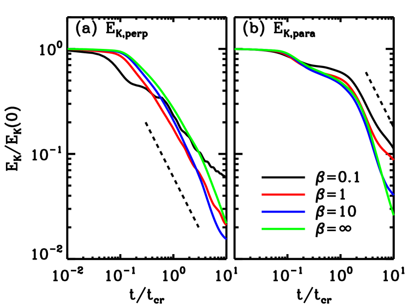
Figure 2: Time evolution of turbulent kinetic energy in the directions (a) perpendicular, $E_{\rm K,perp}/E_{\rm K,perp}(0)$, and (b) parallel, $E_{\rm K,para}/E_{\rm K,para}(0)$, to the initial magnetic field for Series C. Note that $E_{\rm K,perp}=E_{\rm K,x}+E_{\rm K,y}$ is two times greater than $E_{\rm K,para}=E_{\rm K,z}$ at the initial time. The dashed line in each panel denotes a reference line for a power-law form of $E_{\rm K}\propto t^{-1}$.

We separate the turbulent kinetic energy into perpendicular ($E_{\rm K,perp}=E_{\rm K,x}+E_{\rm K,y}$) and parallel ($E_{\rm K,para}=E_{\rm K,z}$) components to the magnetic field direction. Figure 2 plots (a) $E_{\rm K,perp}/E_{\rm K,perp}(0)$ and (b) $E_{\rm K,para}/E_{\rm K,para}(0)$ as a function of time for Series C. Note that $E_{\rm K,perp}$ is two times greater than $E_{\rm K,para}$ initially since the initial velocity field is isotropic in Series C. As shown in panel (b), the parallel component of the kinetic energy is hardly decaying until $t\sim 2t_{\rm cr}$. Since the surrounding WNM has a small density, the CNM expands nearly freely in the vertical direction with less dissipation. After this expansion, the parallel component decays as rapidly as a power-law of $t^{-1}$ irrespective of the field strengths.

However, the perpendicular component of kinetic energy decays similarly to that in Series A; a power-law decay with $E_{\rm K}\propto t^{-1}$ at an early stage and a shallower decay at later times. The strong field model (CS model; black) contains about an order of magnitude more energy at the end of the simulation compared to the CW and CH models, while the remaining energy is significantly dissipated already: at $t/t_{\rm cr}=10$, $E_{\rm K,perp}/E_{\rm K,perp}(0)=5.6\%$, $1.8\%$, $1.4\%$, and $1.6\%$ for the CS, CI, CW, and CH models, respectively.

The evolution of the perturbed magnetic energy also shows a significant difference between the model Series. In Series A, the fluid motions are assigned only in the perpendicular plane to the initial magnetic field. Thus, the perturbed magnetic energy over the whole evolutionary stage is dominated by the parallel component, $\delta B_{z}^{2}$, due to converging and diverging fluid motions. The generation of the perpendicular component, $\delta B_{x}^{2}+\delta B_{y}^{2}$, is limited, especially for the strong field case, where magnetic field lines are hardly bent. Only the AW model has comparable energy in each component at later times. However, in Series B and C, there are non-negligible fluid motions in the direction parallel to the magnetic fields, which generates the perpendicular component of the perturbed magnetic energy as well by stretching and shrinking the field lines. Despite having a different amount of energy stored in each component, the ratios of the total perturbed magnetic energy to the initial turbulent energy at the peak are nearly the same. After (1-3)$t_{\rm cr}$, when the fluid becomes really turbulent with proper scaling relations, $\delta E_{\rm B}$ decays rapidly in Series B and C as $\delta E_{\rm B}\propto t^{-2}$, similar to Ostriker et al. (2001). On the other hand, since the remaining kinetic energy is large enough to keep perturbing the magnetic field at later times, the decay rate of $\delta E_{\rm B}$ in Series A is reduced as well (the power-law exponent is approximately $-1$). The models with weaker field strength in Series B and C maintain their perturbed magnetic energy longer since the magnetic field can be deformed even with weaker fluid motions.

3.1.2 Effect of Boundary Conditions

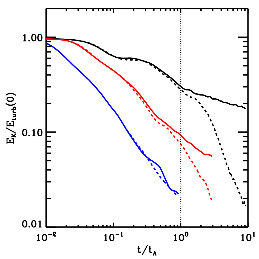
Figure 3: Evolution of turbulent kinetic energy, $E_{\rm K}/E_{\rm turb}(0)$, as a function of time in unit of the Alfvén wave crossing time, $t_{A}=t_{s}(\beta/2)^{1/2}$ where $t_{s}\sim 5t_{\rm cr}$, for the AS (black), AI (red), and AW (blue) models. The solid and dashed lines respectively stand for periodic and continuous BCs at the vertical boundaries. The vertical dotted line denotes $t=t_{A}$.

The models with periodic BCs at the vertical boundaries presented in Section 3.1.1 can be considered as a quasi-global case for CNM sheets that are periodically placed within a large H I cloud. Although there might be many CNM sheets connected with magnetic fields in a H I cloud, the periodic BCs are still an oversimplified assumption. We thus consider another extreme, a single isolated CNM sheet sandwiched by the WNM, by running models with continuous BCs. In this case, waves can escape outward freely. We only consider models in Series A with continuous BCs since Series B is not much affected by vertical boundaries, and Series C is inappropriate to run with continuous BCs due to the initial vertical expansion, which would induce significant mass loss with continuous BCs.

Figure 3 shows the time evolution of the normalized turbulent kinetic energies $E_{\rm K}/E_{\rm turb}(0)$ for the AS (black), AI (red), and AW (blue) models with periodic (solid) and continuous (dotted) BCs at the vertical boundaries, $z=\pm L_{z}/2$. Here, the time is normalized by the Alfvén wave crossing time $t_{A}$, which differs for each model. The kinetic energy evolution begins to differ at around $t=t_{A}$. After one Alfvén wave crossing time, the overall evolution is greatly affected by the BCs; the turbulent energy decays very rapidly with continuous BCs.

Since the initial velocity perturbations in Series A are assigned in the perpendicular plane to the initial magnetic field, Alfvén waves are excited initially and propagate toward the WNM along the field lines. They are not dissipative themselves and hardly produce compressible waves (slow and fast waves) since the mode coupling is in general very weak (e.g., Cho et al., 2002; Cho & Lazarian, 2003). It is evident in Figure 3 that travelling Alfvén waves that reenter to the CNM sheet after one Alfvén wave crossing time are responsible for the reduced decay rates observed in the AS and AI models. Even with a strong magnetic field, the decay rate of turbulence cannot be reduced for a single, isolated CNM sheet by storing energy in Alfvén waves, as has long been considered since Arons & Max (1975). Rather, it seems that maintaining and/or replenishing mechanisms for the Alfvén waves are necessary to obtain a reduced decay rate.

3.2 Turbulence Characteristics

In Section 3.1, we find not only consistent results with previous local isothermal simulations for early decay of turbulent kinetic energy, but also new results of decaying turbulence with reduced rates in the XY plane when the field is vertical and strong. Since weak field models are similar to hydrodynamic models and previous local simulations, here we put more emphasis on strong field models for a detailed analysis of turbulence characteristics. Note that the intermediate field models also show similar characteristics to the strong field models, but with less residual energy.

3.2.1 AS Model

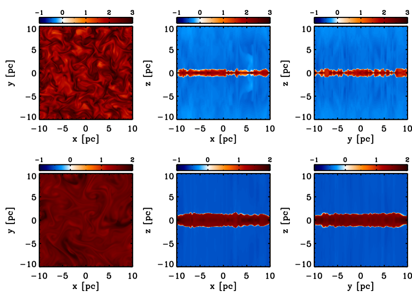
Figure 4: Number density slices in logarithmic color scales at $z=0$ (left), $y=0$ (middle), and $x=0$ (right) for the AS model at $t/t_{\rm cr}=1$ (top) and $10$ (bottom). Note that we adjust the color schemes in the color bars above each panel to associate a white color with the maximum number density of the WNM ($n=1\;{\rm cm}^{-3}$) for a clearer distinction between the WNM and CNM (plus unstable phase). Bluish and reddish colors denote the WNM and CNM (plus unstable phase), respectively.

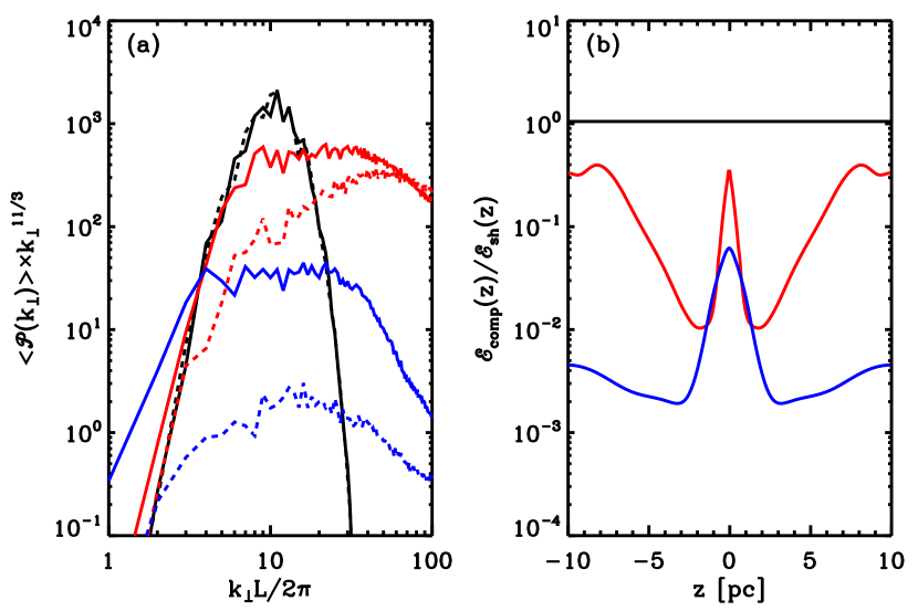
Figure 5: (a) Cylindrically-binned, vertically-integrated PS of the AS model at $t/t_{\rm cr}=0$ (black), $1$ (red), and $10$ (blue). The solid and dashed lines stand for the shearing and compressible components, respectively. See Eq.(13) and text for details. (b) Ratios between the compressible and shearing components of the specific energy integrated over $k_{\perp}$ as a function of $z$. See Eq.(14) and text for details.

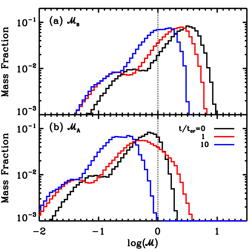
Figure 6: (a) Sonic and (b) Alfvén Mach number PDFs for the AS model. The vertical dotted line denotes a Mach number of unity.

In order to investigate the characteristics of the remaining turbulence at later times, we begin by analysing the AS model with periodic BCs since it has a significant amount of energy at later times compared to the others. Figure 4 shows number density snapshots for the AS model in the XY plane at $z=0$ (left), the $\hat{\mathbf{x}}$-$\hat{\mathbf{z}}$ plane at $y=0$ (XZ plane; middle), and the $\hat{\mathbf{y}}$-$\hat{\mathbf{z}}$ plane at $x=0$ (YZ plane; right) at $t/t_{\rm cr}=1$ (top) and $10$ (bottom). In the XY plane, it is clearly shown that there are strong shocks within the CNM sheet at an early stage due to compressible motions with supersonic velocity (top-left), while the remaining motions are less compressive but vortical (bottom-left). Note that the snapshots at $t/t_{\rm cr}=1$ may not reflect the saturated state of turbulence but illustrate a particular choice of our initial conditions, since the saturated state of turbulence would be achieved (2-3)$t_{\rm cr}$ after driving begins (e.g., Stone et al., 1998). Vertical motions are also induced due to a velocity difference at the contact discontinuity of the two phases, but they are negligible. The thickness of the CNM sheet is slightly increased (middle and right).

For a more quantitative analysis, we decompose the velocity fields into shearing (divergence-free) and compressible (curl-free) components by using a Helmholtz decomposition (e.g., Kowal & Lazarian 2010). As seen in the middle and right panels of Figure 4, the background density of the AS model is varying as a function of $z$, and induced vertical motions are negligible. A cylindrically-binned PS would thus give good characteristics at all evolutionary stages for the AS model. This analysis is advantageous to see how the PS varies along the vertical direction, while it is not suitable to address anisotropy of turbulence since it shows the $k_{z}=0$ mode only. We first take a 2D FFT in the XY plane for $v_{x}$ and $v_{y}$ at a given vertical position. The shearing and compressible components of the velocity PS can then be obtained as functions of $z$ and $k_{\perp}$ by

$$\mathcal{P}_{\rm sh}(k_{\perp};z)=|\mathbf{\hat{k}}_{R}\times\tilde{\mathbf{v}}(\mathbf{k}_{\perp};z)|^{2}\quad\textrm{and}\quad\mathcal{P}_{\rm comp}(k_{\perp};z)=|\mathbf{\hat{k}}_{R}\cdot\tilde{\mathbf{v}}(\mathbf{k}_{\perp};z)|^{2},$$ (12)

where $\tilde{\mathbf{v}}$ is the velocity field in the Fourier space, $\mathbf{k_{\perp}}=(k_{x},k_{y})$ is the wave vector in the perpendicular (XY) plane, and $k_{\perp}=(k_{x}^{2}+k_{y}^{2})^{1/2}$ is the cylindrically-binned wavenumber. Since our main interests focus on turbulence within the CNM, we calculate a mass-weighted, vertically-averaged PS for each component as

$$\left\langle{\mathcal{P}(k_{\perp})}\right\rangle=\frac{\int\overline{\rho}(z)\mathcal{P}(k_{\perp};z)dz}{\int\overline{\rho}(z)dz},$$ (13)

where $\overline{\rho}(z)=\int\rho dxdy/(L_{x}L_{y})$ is the horizontally-averaged density. We also calculate a specific energy for each component as a function of $z$:

$$\mathcal{E}(z)=\frac{1}{2}\int\mathcal{P}(k_{\perp};z)\pi k_{\perp}dk_{\perp}.$$ (14)

Figure 5 plots (a) $\left\langle{\mathcal{P}_{\rm sh}(k_{\perp})}\right\rangle\times k_{\perp}^{11/3}$ (solid) and $\left\langle{\mathcal{P}_{\rm comp}(k_{\perp})}\right\rangle$ (dashed) as a function of $k_{\perp}$ and (b) $\mathcal{E}_{\rm comp}(z)/\mathcal{E}_{\rm sh}(z)$ as a function of $z$ at $t/t_{\rm cr}=0$ (black), $1$ (red), and $10$ (blue) for the AS model. In order to show the slope and inertial range of the PS clearly, we multiply $k_{\perp}^{11/3}$ in panel (a) to the PS. Initially, the same amount of energy is assigned in the shearing and compressible components (see black line in Figure 5(b)). The compressible component keeps decaying rapidly due to strong shock dissipation, while the shearing component survives longer as seen in Figure 5(a) (see also left panels of Figure 4). As time goes by, the power diffuses to larger scales via the inverse cascade, and the shearing mode at larger scales starts growing and finally dominates, while at small scales both the compressible and shearing components keep decaying. The shearing component of the PS at $t/t_{\rm cr}=10$ (the final time of simulation) follows a power-law shape with an exponent of $-11/3$ in an inertial range of $4\leq k_{\perp}L/2\pi\leq 20$. The slope is consistent with the expected value in incompressible hydrodynamic and MHD turbulence (Kolmogorov, 1941; Goldreich & Sridhar, 1995), which is also known to be applicable to Alfvén modes (as well as slow modes) in compressible MHD turbulence (Cho & Lazarian, 2003). This slope is achieved and preserved after one crossing time, while the inertial range varies. The remaining turbulent energy within the CNM sheet at later times in the AS model is thus mostly in the form of incompressible motions and cascades from larger to smaller scales as in traditional incompressible turbulence. It is not everlasting as in purely thin-disk models with a potential field outside (Basu & Dapp, 2010).

It is evident that incompressible motions in the direction perpendicular to the CNM sheet survive longer and are responsible for the reduced decay rate. Initial velocity perturbations deform magnetic fields, and a part of the perturbed kinetic energy is stored in the form of magnetic energy. Since the Alfvén waves excited by motions in the direction perpendicular to the magnetic field cannot escape the simulation domain with periodic BCs, they reenter the CNM sheet and help to preserve shearing motions in the CNM sheet. After one Alfvén wave crossing time, the evolution of turbulent energy within the CNM sheet is affected by the reentering waves and shows a reduced decay rate (see Figure 3).

The mean energy ratios between the compressible and shearing components, $\int\mathcal{E}_{\rm comp}(z)dz/\int\mathcal{E}_{\rm sh}(z)dz$, are $16\%$ and $0.8\%$ at $t/t_{\rm cr}=1$ and $10$, respectively. However, within the CNM sheet (at around $z=0$), the energy in the compressible mode remains up to $35\%$ and $6\%$ of the shearing mode energy at $t/t_{\rm cr}=1$ and $10$, respectively. At the final snapshot, the energy ratio at the midplane is about an order of magnitude greater than at higher-$|z|$. Since the amplitude of incompressible motions is still supersonic within the CNM sheet (see Figure 6), the more compressible mode can be more easily generated than in the WNM. However, the generation of compressible modes by incompressible Alfvén waves is limited (Cho et al., 2002; Cho & Lazarian, 2003) so that the energy ratio is still very small (only a few percents) even within the CNM sheet.

Since our model is not isothermal, the probability distribution functions (PDFs) of sonic and Alfvén Mach numbers provide better understanding of the velocity dispersions of each gas phase. The Mach numbers for each gas parcel are defined by $\mathcal{M}_{s}\equiv v_{\rm 1D}/c_{s}$ and $\mathcal{M}_{A}\equiv v_{\rm 1D}/v_{A}$, where $v_{\rm 1D}\equiv[(v_{x}^{2}+v_{y}^{2})/2]^{1/2}$, $c_{s}\equiv(P/\rho)^{1/2}$, and $v_{A}\equiv B/(4\pi\rho)^{1/2}$. Note that we ignore the velocity in the vertical direction $v_{z}$, which is negligibly small compared to $v_{x}$ and $v_{y}$ at all times in the AS model. Figure 6 plots mass fractions of gas in the AS model for (a) sonic and (b) Alfvén Mach numbers to put more emphasis on the CNM. For $\beta=0.1$, initial mean Mach numbers for the CNM are $\mathcal{M}_{s}=\sigma_{\rm 1D,0}/c_{c}\sim 3.3$ and $\mathcal{M}_{A}=\sigma_{\rm 1D,0}/v_{A,c}\sim 0.75$. However, as seen in Figure 6(b), about $32\%$ of the CNM by mass is in the super-Alfvénic regime initially. Overall the PDFs gradually move toward smaller values as $v_{\rm 1D}$ decreases. In the high density tail of the $\mathcal{M}_{A}$-PDF, $\mathcal{M}_{A}$ is initially increased even though $v_{\rm 1D}$ keeps decreasing. This is due to an initial lowering of $v_{A}$ for the densest gas since there are not only horizontal motions but also vertical compression (see top panels of Figure 4), which enhances density but not magnetic field energy. At $t/t_{\rm cr}=10$, $66\%$ of the CNM by mass is still supersonic, but the entire gas is sub-Alfvénic.

3.2.2 BS and CS Models

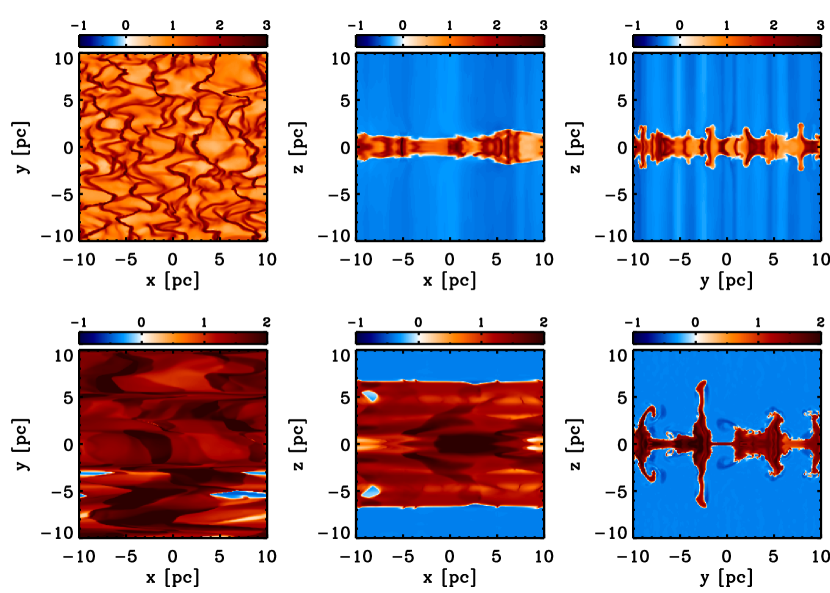
Figure 7: Same as Figure 4, but for the BS model. Note that middle panels are slices along $y=-2.9\;{\rm pc}$ (not $y=0\;{\rm pc}$) to show the structure of the sheet in the XZ plane.

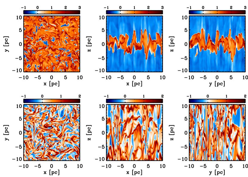
Figure 8: Same as Figure 4, but for the CS model.

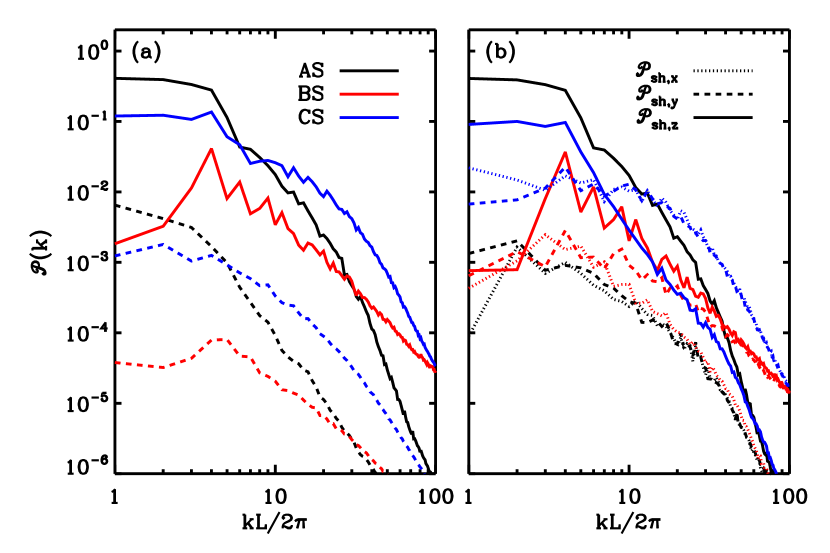
Figure 9: (a) Spherically-binned PS for the shearing (solid) and compressible (dashed) components for $\beta=0.1$ models at $t/t_{\rm cr}=10$. (b) Directionally-decomposed PS for the shearing components.

Figures 7 and 8 show number density slices in logarithmic color scales for the BS and CS models, respectively, as in Figure 4. In contrast to the AS model, the initial CNM sheet is not maintained, due to non-negligible vertical motions in both models. The structures in the BS and CS models are greatly different from one another.

Since the gas can flow more easily along the magnetic field lines, the initial motions in the XY plane for the BS model soon become anisotropic. The kinetic energies in the $\hat{\mathbf{y}}$- and $\hat{\mathbf{z}}$-directions become comparable after $t=t_{\rm cr}$, while the remaining energy, which keeps decaying rapidly (in contrast to the AS and CS models), is deposited to gas flows in the $\hat{\mathbf{x}}$-direction. At $t=t_{\rm cr}$, filaments in the CNM sheet align to the $\hat{\mathbf{y}}$-direction in the XY plane, perpendicular to the initial magnetic field (see top-left panel of Figure 7). Initially formed filaments keep moving, colliding, and merging along the $\hat{\mathbf{x}}$-direction. These overdense regions are soon smeared out along the $\hat{\mathbf{x}}$-direction but preserved in the $\hat{\mathbf{y}}$-direction. Thus, overdense regions then expand vertically and form vertical sheets in the XZ plane (see middle and right panels of Figure 7).

As we noted in the kinetic energy evolution of Series C (Figure 2), initial vertical turbulent motions induce an overall expansion of the CNM sheet due to (turbulent) pressure imbalance. It is clearly seen in the top panels of Figure 8. After about $t/t_{\rm cr}=2$, the CNM and WNM are mixed up completely and coexist at all vertical positions. The turbulent energy in the XY plane decays a bit longer than in the AS model, and incompressible motions at large scales eventually dominate. In the bottom panels of Figure 8, predominant vortical motions are evident in the XY plane as in Figure 4, while the vertically stretched CNM is shown in the XZ and YZ planes.

By comparing the AS and BS models, we see that the initial magnetic field direction results in drastic differences for turbulent energy and structural evolution. On the other hand, there are many similarities between the AS and CS models despite the substantial structural difference in the vertical slices. In order to characterize turbulence quantitatively, we again investigate the velocity PS using the Helmholtz decomposition. For the BS and CS models, the vertical motions at later times are not negligible, so that the plane-parallel PS analysis done in Section 3.2.1 is not suitable. It is better to use velocity fields in full three dimensions. We decompose the velocity fields in Fourier space in a similar manner but for a three-dimensional wave vector $\mathbf{k}=(k_{x},k_{y},k_{z})$ and spherically-binned wavenumber $k=(k_{x}^{2}+k_{y}^{2}+k_{z}^{2})^{1/2}$ (see Eq.(12)). There is no additional averaging needed for a spherically-binned PS. Note that the shearing component of the PS in three dimensions has three components, representing the power of incompressible motions perpendicular to the each axis, referred to as $\mathcal{P}_{\rm sh,x}$, $\mathcal{P}_{\rm sh,y}$, and $\mathcal{P}_{\rm sh,z}$.

Figure 9 plots the spherically-binned PS of the AS (black), BS (red), and CS (blue) models at $t/t_{\rm cr}=10$. In panel (a), the shearing (solid) and compressible (dashed) components are shown as in Figure 5(a). Note that for the AS model, $\mathcal{P}_{\rm sh}$ is almost identical to that in Figure 5(a), while $\mathcal{P}_{\rm comp}$ shows slightly smaller power at large scales (small $k_{\perp}$ and $k$). This is because the analysis does not give a mass-weighted velocity PS, but rather a volume-weighted PS that originates not from the CNM but from the WNM. There is a clear signature of the enhanced incompressible component at large scales for the CS model, while there is no such a feature in the BS model. The ratios of the compressible to incompressible components of the integrated specific energy, $\mathcal{E}_{\rm comp}/\mathcal{E}_{\rm sh}=\int\mathcal{P}_{\rm comp}(k)4\pi k^{2}dk/\int\mathcal{P}_{\rm sh}(k)4\pi k^{2}dk$, are about $1\%$ for all models, again implying that the compressible component is hardly generated by incompressible Alfvén waves.

In Figure 9(b), we plot the shearing component of the PS perpendicular to each wave vector. For the AS model, it is clearly seen that the shearing component perpendicular to the magnetic field, $\mathcal{P}_{\rm sh,z}$, is dominant at all scales, justifying our plane-parallel analysis in Section 3.2.1. For the CS model, $\mathcal{P}_{\rm sh,z}$ (blue solid) is remarkably similar to that in the AS model with slightly lower power despite a non-negligible $\mathcal{P}_{\rm sh,x}$ and $\mathcal{P}_{\rm sh,y}$ in the CS model. This again implies a Kolmogorov-like scaling $\mathcal{P}\propto k_{\perp}^{-11/3}$ as in Cho & Lazarian (2003). Most of energy is deposited into larger scales so that slowly decaying kinetic energy at later times is mainly due to the large-scale shearing component in the direction perpendicular to the magnetic field, as in the AS model.

The characteristics of turbulence in the BS model are quite different from those of the AS and CS models, as expected. The shearing component still dominates the compressible component, but there is no clear enhancement of large scale modes. For the shearing component, the perpendicular component ($\mathcal{P}_{\rm sh,x}$) has less energy than the parallel components, in stark contrast to the AS and CS models, whose energy is mainly dominated by the perpendicular component ($\mathcal{P}_{\rm sh,z}$).

4 Discussion

Based on numerous local isothermal simulations of decaying MHD turbulence during the last two decades, it has been widely accepted that compressible MHD turbulence in the ISM is decaying rapidly regardless of magnetic field strength. Due to inherent limitations of local modeling, however, the effects of global structures of magnetic fields and the diffuse multiphase ISM have not been explored. Idealized two-dimensional models of thin sheets with magnetic fields anchored in the interstellar space have shown self-sustained turbulence driven by the global MHD effect (magnetic-tension driven mode) in a flux-freezing limit (Basu & Dapp, 2010). In this paper, we extend their models to more realistic interstellar conditions, consisting of thin CNM sheets embedded in low density WNM (Heiles & Troland, 2003, 2005). By solving interstellar cooling and heating explicitly with a set of ideal MHD equations, we are able to investigate long-term evolution of turbulent energy decay and characteristics of the remaining energy in the diffuse multiphase ISM.

In contrast to the idealized models of Basu & Dapp (2010), who assumed instantaneous field redistribution toward a potential field outside thin sheets, the kinetic energy in our models cannot persist (see also Kudoh & Basu 2011). The initial evolution of the kinetic energy is rather similar to local models characterized by the decay times shorter than a flow crossing time and power-law shape decay of $E\propto t^{-1}$ (e.g., Mac Low et al. 1998; Stone et al. 1998). For our strong field model (AS model) with vertical magnetic fields and anisotropic turbulence (no initial vertical motions), we find a clear signature of reduced decay rate at later times, and the kinetic energy remains at $32\%$ and $18\%$ of the initial energy at $t/t_{\rm cr}=1$ and $10$, respectively. Similar results are found in the weaker field models, but less energy remains for weaker magnetic fields (Figure 1(a)). This dependence on the field strengths is also shown in Series C (with vertical fields and isotropic turbulence), while turbulent energy keeps decaying as a power-law of $E\propto t^{-1}$ in Series B (with horizontal fields and anisotropic turbulence) irrespective of magnetic field strengths (Figure 1(b) and (c)). In Ostriker et al. (1999), two-dimensional local models with horizontal magnetic fields have also reported reduced decay rates for strong magnetic fields, arising mainly from a lack of dissipation in the symmetric direction (see also Gammie 1996; Kudoh & Basu 2003). Although the initial velocity fields are two-dimensional in Series A and B, vertical motions emerge naturally since there is no artificial suppression of dissipation in the symmetric direction. The reduced decay rates shown in the AS and CS models are indeed due to the survival of incompressible motions in the direction perpendicular to the magnetic field (see Section 3.2).

We use the Helmholtz decomposition method to obtain incompressible and compressible components of the velocity PS, providing detailed characteristics of the remaining turbulence. At later times, almost all the energy in Series A and C is in the form of shearing motions perpendicular to the magnetic field (in the XY plane) at the largest scale (Figure 9). The remaining energy in the compressible component has only $1\%$ of the incompressible component at the end of simulation ($t/t_{\rm cr}=10$), while the CNM sheets contain more compressible energy than the WNM (Figure 5). Although a significant fraction of the CNM by mass is in supersonic regimes, incompressible Alfvén waves are hardly generating compressible motions, implying a weak coupling of MHD waves in the absence of driving (c.f., Cho et al. 2002; Cho & Lazarian 2003). The velocity PS for the AS and CS models at later times show power-law shapes $\mathcal{P}_{\rm sh}\propto k^{-11/3}$, close to that in classical incompressible turbulence (Kolmogorov, 1941; Goldreich & Sridhar, 1995). This is not surprising since Alfvén modes (and slow modes as well) follow a Kolmogorov-like spectrum (Cho et al., 2002; Cho & Lazarian, 2003), and these are the dominant modes in our simulations.

Based on our models, we find for the AS model (and also the CS model) a significant delay of turbulent decay and non-negligible remaining turbulent energy ($v_{\rm 1D}\sim 1\;{\rm km}\;{\rm s}^{-1}$), which may be associated with supersonic non-thermal linewidths within the CNM. This requires a sheet-like CNM distribution with strong magnetic fields threading perpendicular to the sheet, as well as periodic BCs in the vertical direction. For a typical thermal pressure of the diffuse ISM, $P_{0}/k_{\rm B}\sim 3-4\times 10^{3}\;{\rm cm}^{-3}\,{\rm K}$ in the Solar neighborhood (Jenkins & Tripp, 2001, 2011; Wolfire et al., 2003), a strong magnetic field assumed in the AS model ($\beta=0.1$) implies $B_{0}\sim 10-12\;\mu{\rm G}$ (see Eq.(9)). The observed average strength of the total magnetic field in spiral galaxies is about $10\;\mu{\rm G}$, while weaker fields ($\sim 5\;\mu{\rm G}$) are observed for radio-faint galaxies in the Local group, and star-forming galaxies show stronger field strengths of $20$-$30\;\mu{\rm G}$ (see Beck 2005 and references therein). The median value of the CNM ($10\;{\rm cm}^{-3}<n_{\rm H}<300\;{\rm cm}^{-3}$) in the Milky Way is about $6\;\mu{\rm G}$ (Heiles & Troland, 2005; Crutcher et al., 2010; Crutcher, 2012). Thus the typical magnetic field strengths in the ISM are generally expected to be in the strong-field regime with respect to the thermal pressure, as in the AS model.

A sheet-like CNM perpendicular to the local magnetic field is also expected to be common. One direct formation mechanism for CNM structure is condensation of the WNM due to supersonic colliding flows driven by e.g., supernova explosions. Recent simulations of supersonic colliding flows with magnetic fields by Heitsch et al. (2009) show that a thin CNM sheet perpendicular to the field can be formed when the WNM flows along a strong magnetic field, otherwise sheets are soon disrupted by the nonlinear thin shell instability (Vishniac, 1994; Heitsch et al., 2007). In numerical simulations of structure formation in the multiphase ISM solely by thermal instability, CNM filaments or sheets are usually formed along the direction perpendicular to the field lines since gas flows across the field are prevented, especially in strong field cases (e.g., Hennebelle & Pérault 2000; Inoue & Inutsuka 2012). When CNM clouds are formed by large-scale gravitational collapse within slightly supercritical gas, planar structures perpendicular to the magnetic field direction are also expected to form first. Subsequently, self-gravity overwhelms other forces, such as magnetic-tension, in order to cause isotropic collapse. In a high-resolution H I absorption line survey using the Arecibo radio telescope, Heiles & Troland (2003) have suggested “blobby sheets” to characterize the structure of CNM clouds rather than isotropic clouds (see also Gibson et al. 2000; Meyer et al. 2006), while the orientation of the magnetic fields is still uncertain (Heiles & Troland, 2005).

Such commonly observed CNM sheets imply that the CNM and WNM should be in total pressure equilibrium in direction perpendicular to the sheet, otherwise the sheet is dispersed easily as seen in Series C (see Figure 8). The total pressure equilibrium can be expressed as

$$P_{\rm th,w}+P_{\rm turb,w}+\delta P_{\rm mag,w}=P_{\rm th,c}+P_{\rm turb,c}+\delta P_{\rm mag,c},$$ (15)

where $P_{\rm th}=\rho c_{s}^{2}$, $P_{\rm turb}=\rho\sigma_{z}^{2}$, and $\delta P_{\rm mag}=\delta B^{2}/8\pi$ are the thermal, turbulent, and turbulent magnetic pressures, respectively. Subscripts ‘w’ and ‘c’ represent the WNM and CNM, respectively. Assuming that the density, temperature, vertical velocity dispersion, turbulent magnetic fields are constant within each gas phase, Eq.(15) results in a thermal pressure ratio between the two phases

$$\mathcal{R}_{p}\equiv\frac{P_{\rm th,w}}{P_{\rm th,c}}=\frac{1+\mathcal{M}_{c}^{2}+\beta_{c}^{-1}}{1+\mathcal{M}_{w}^{2}+\beta_{w}^{-1}}.$$ (16)

The left hand side of Eq.(16) can be constrained by thermal equilibrium. For given interstellar cooling and heating rates, there are maximum and minimum thermal pressures of the WNM and CNM, $P_{\rm max}$ and $P_{\rm min}$, respectively, and $P_{\rm max}\sim 3P_{\rm min}$ (Wolfire et al., 1995, 2003). Since the cooling time scale is generally short compared to the gas dynamical time scales, gas is expected to be in thermal equilibrium even in the case of vigorously turbulent disks (e.g., Piontek & Ostriker 2005; Kim et al. 2011). Thus, it is likely to have $\mathcal{R}_{p}<3$. More generally, the CNM can have higher thermal pressure due to self-gravity (e.g., Jenkins & Tripp 2011) so that it is more natural to have $\mathcal{R}_{p}\lower 2.15277pt\hbox{$\;\buildrel<\over{\sim}\;$}1$.

Non-thermal linewidths in the CNM and WNM are observed in the ranges of $\sim 2-7\;{\rm km}\;{\rm s}^{-1}$ and $\lower 2.15277pt\hbox{$\;\buildrel>\over{\sim}\;$}10\;{\rm km}\;{\rm s}^{-1}$, respectively, resulting in $\mathcal{M}_{c}>3$ and $\mathcal{M}_{w}\sim 1$-$2$ (Heiles & Troland, 2003; Kalberla & Kerp, 2009). If the magnetic field is uniform and perpendicular to the sheet, we can neglect a contribution from magnetic pressure. We then have the thermal pressure ratio $\mathcal{R}_{p}>5$ for $\mathcal{M}_{c}>3$ and $\mathcal{M}_{w}\sim 1$ from the observed velocity dispersions, which is inconsistent with the expectation from thermal equilibrium of the multiphase ISM. If the turbulence within CNM sheets is anisotropic so that the turbulent pressure in the parallel direction to the field is negligible as in Series A and B, $\mathcal{R}_{p}$ can be kept around unity with the observed Mach numbers of each medium. There are also other ways to explain this contradiction. If CNM sheets are confined mainly by the ram pressure of the WNM as in colliding flow simulations, an additional term appears in denominator of Eq.(16), reducing $\mathcal{R}_{p}$ if the Mach number of the colliding flow is similar to $\mathcal{M}_{c}$ (e.g., Heitsch et al. 2009). It is also possible to have isotropic turbulence in sheets if the turbulent magnetic pressure overwhelms other terms and $\beta_{c}\lower 2.15277pt\hbox{$\;\buildrel>\over{\sim}\;$}\beta_{w}$. Although the turbulent magnetic field can be as strong as the uniform field (Heiles & Troland, 2005; Han et al., 2006), anisotropic turbulence is still preferred since $\beta\sim 0.3$ is not enough to overwhelm turbulent terms.

As we have shown in Section 3.1.2, an isolated CNM sheet (modelled by continuous BCs) cannot maintain the turbulent energy for a longer time. Instead, the energy decays rapidly as in local simulations. The reduced decay rate found in the AS model is thus a consequence of the replenishment of Alfvén waves into the CNM sheet caused by the periodic BCs. In the real ISM, the CNM sheets would be neither placed periodically in the direction perpendicular to the magnetic field nor would they be isolated. Realistic global simulations that model larger magnetized, multiphase H I clouds containing a number of CNM sheets would be necessary to further investigate the reduced decay rate of turbulence found in the AS model.

In this paper, we focus on the long-term evolution of decaying turbulence under the influence of interstellar cooling and heating with global structures of magnetic fields. In reality, however, dynamical processes whose time scales are shorter than the decay time of turbulence should be taken into account to explore dynamical and structural evolution of the multiphase ISM. Using a driving scheme in Fourier space, several studies have explored characteristics of turbulence in the multiphase ISM, such as density and pressure PDFs, mass fractions, structure functions, and power spectra (e.g., Gazol et al. 2005; Gazol & Kim 2010, 2013; Seifried et al. 2011; Saury et al. 2013). More realistic situations have also been considered with driving sources of turbulence such as converging flows (e.g., Audit & Hennebelle 2005, 2010; Hennebelle & Audit 2007; Heitsch et al. 2005, 2009; Vázquez-Semadeni et al. 2007) and propagating shock waves (e.g., Koyama & Inutsuka 2000, 2002). Since only a few of them considered the effect of magnetic fields (e.g, Gazol et al. 2009; Heitsch et al. 2009; Hennebelle & Pérault 2000; Hennebelle & Inutsuka 2006), however, many MHD turbulence characteristics within the multiphase ISM remain unexplored. Especially, driven turbulence within CNM sheets with self-gravity can be investigated in our future work.

5 Summary

Using three-dimensional ideal MHD simulations with interstellar cooling and heating, we have shown that the long-term evolution of decaying turbulence in CNM sheets embedded in a WNM can be different from the usual results of local isothermal simulations. Both models share common characteristics of decaying turbulence described by power-law decay with short decay time at early evolutionary stages. For strong and perpendicular (to the sheet) magnetic fields however, turbulent kinetic energy decays slowly at later times and can survive longer until $10t_{\rm cr}$ in the form of incompressible motions in the plane of the sheet. A significant amount of energy, $\sim 20\%$ of the initial energy, remains in models with strong fields ($\beta=0.1$) and anisotropic velocity perturbations (no initial vertical motions; AS model). One more very important requirement for a longer-lived turbulence maintained by a strong magnetic field is a mechanism to compensate for the leaking of Alfvén waves (periodic BCs in our models). While idealized, such BCs may represent some aspects of the interaction of multiple CNM sheets within the observed neutral ISM (Heiles & Troland, 2005).

References

- Arons & Max (1975) Arons, J., & Max, C. E. 1975, ApJ, 196, L77
- Audit & Hennebelle (2005) Audit, E., & Hennebelle, P. 2005, A&A, 433, 1
- Audit & Hennebelle (2010) —. 2010, A&A, 511, A76
- Basu & Dapp (2010) Basu, S., & Dapp, W. B. 2010, ApJ, 716, 427
- Beck (2005) Beck, R. 2005, in Lecture Notes in Physics, Berlin Springer Verlag, Vol. 664, Cosmic Magnetic Fields, ed. R. Wielebinski & R. Beck, 41
- Cho & Lazarian (2003) Cho, J., & Lazarian, A. 2003, MNRAS, 345, 325
- Cho et al. (2002) Cho, J., Lazarian, A., & Vishniac, E. T. 2002, ApJ, 564, 291
- Cho & Vishniac (2000) Cho, J., & Vishniac, E. T. 2000, ApJ, 539, 273
- Crutcher (2012) Crutcher, R. M. 2012, ARA&A, 50, 29
- Crutcher et al. (2010) Crutcher, R. M., Wandelt, B., Heiles, C., Falgarone, E., & Troland, T. H. 2010, ApJ, 725, 466
- Elmegreen (1985) Elmegreen, B. G. 1985, ApJ, 299, 196
- Elmegreen & Scalo (2004) Elmegreen, B. G., & Scalo, J. 2004, ARA&A, 42, 211
- Evans & Hawley (1988) Evans, C. R., & Hawley, J. F. 1988, ApJ, 332, 659
- Field et al. (1969) Field, G. B., Goldsmith, D. W., & Habing, H. J. 1969, ApJ, 155, L149
- Gammie (1996) Gammie, C. F. 1996, ApJ, 462, 725
- Gammie & Ostriker (1996) Gammie, C. F., & Ostriker, E. C. 1996, ApJ, 466, 814
- Gazol & Kim (2010) Gazol, A., & Kim, J. 2010, ApJ, 723, 482
- Gazol & Kim (2013) —. 2013, ApJ, 765, 49
- Gazol et al. (2009) Gazol, A., Luis, L., & Kim, J. 2009, ApJ, 693, 656
- Gazol et al. (2005) Gazol, A., Vázquez-Semadeni, E., & Kim, J. 2005, ApJ, 630, 911
- Gibson et al. (2000) Gibson, S. J., Taylor, A. R., Higgs, L. A., & Dewdney, P. E. 2000, ApJ, 540, 851
- Goldreich & Sridhar (1995) Goldreich, P., & Sridhar, S. 1995, ApJ, 438, 763
- Han et al. (2006) Han, J. L., Manchester, R. N., Lyne, A. G., Qiao, G. J., & van Straten, W. 2006, ApJ, 642, 868
- Heiles & Troland (2003) Heiles, C., & Troland, T. H. 2003, ApJ, 586, 1067
- Heiles & Troland (2005) —. 2005, ApJ, 624, 773
- Heitsch et al. (2005) Heitsch, F., Burkert, A., Hartmann, L. W., Slyz, A. D., & Devriendt, J. E. G. 2005, ApJ, 633, L113
- Heitsch et al. (2007) Heitsch, F., Slyz, A. D., Devriendt, J. E. G., Hartmann, L. W., & Burkert, A. 2007, ApJ, 665, 445
- Heitsch et al. (2009) Heitsch, F., Stone, J. M., & Hartmann, L. W. 2009, ApJ, 695, 248
- Hennebelle & Audit (2007) Hennebelle, P., & Audit, E. 2007, A&A, 465, 431
- Hennebelle & Inutsuka (2006) Hennebelle, P., & Inutsuka, S.-i. 2006, ApJ, 647, 404
- Hennebelle & Pérault (2000) Hennebelle, P., & Pérault, M. 2000, A&A, 359, 1124
- Inoue & Inutsuka (2012) Inoue, T., & Inutsuka, S.-i. 2012, ApJ, 759, 35
- Jenkins & Tripp (2001) Jenkins, E. B., & Tripp, T. M. 2001, ApJS, 137, 297
- Jenkins & Tripp (2011) —. 2011, ApJ, 734, 65
- Kalberla & Kerp (2009) Kalberla, P. M. W., & Kerp, J. 2009, ARA&A, 47, 27
- Kim et al. (2008) Kim, C.-G., Kim, W.-T., & Ostriker, E. C. 2008, ApJ, 681, 1148
- Kim et al. (2011) —. 2011, ApJ, 743, 25
- Kolmogorov (1941) Kolmogorov, A. 1941, Akademiia Nauk SSSR Doklady, 30, 301
- Kowal & Lazarian (2010) Kowal, G., & Lazarian, A. 2010, ApJ, 720, 742
- Koyama & Inutsuka (2000) Koyama, H., & Inutsuka, S. 2000, ApJ, 532, 980
- Koyama & Inutsuka (2002) —. 2002, ApJ, 564, L97
- Kritsuk & Norman (2002) Kritsuk, A. G., & Norman, M. L. 2002, ApJ, 569, L127
- Kritsuk & Norman (2004) —. 2004, ApJ, 601, L55
- Kudoh & Basu (2003) Kudoh, T., & Basu, S. 2003, ApJ, 595, 842
- Kudoh & Basu (2006) —. 2006, ApJ, 642, 270
- Kudoh & Basu (2011) —. 2011, ApJ, 728, 123
- Larson (1981) Larson, R. B. 1981, MNRAS, 194, 809
- Lithwick & Goldreich (2001) Lithwick, Y., & Goldreich, P. 2001, ApJ, 562, 279
- Mac Low & Klessen (2004) Mac Low, M., & Klessen, R. S. 2004, Reviews of Modern Physics, 76, 125
- Mac Low et al. (1998) Mac Low, M., Klessen, R. S., Burkert, A., & Smith, M. D. 1998, Physical Review Letters, 80, 2754
- Maron & Goldreich (2001) Maron, J., & Goldreich, P. 2001, ApJ, 554, 1175
- McKee & Ostriker (2007) McKee, C. F., & Ostriker, E. C. 2007, ARA&A, 45, 565
- Meyer et al. (2006) Meyer, D. M., Lauroesch, J. T., Heiles, C., Peek, J. E. G., & Engelhorn, K. 2006, ApJ, 650, L67
- Ostriker et al. (1999) Ostriker, E. C., Gammie, C. F., & Stone, J. M. 1999, ApJ, 513, 259
- Ostriker et al. (2001) Ostriker, E. C., Stone, J. M., & Gammie, C. F. 2001, ApJ, 546, 980
- Padoan & Nordlund (1999) Padoan, P., & Nordlund, Å. 1999, ApJ, 526, 279
- Piontek & Ostriker (2004) Piontek, R. A., & Ostriker, E. C. 2004, ApJ, 601, 905
- Piontek & Ostriker (2005) —. 2005, ApJ, 629, 849
- Saury et al. (2013) Saury, E., Miville-Deschênes, M.-A., Hennebelle, P., Audit, E., & Schmidt, W. 2013, arXiv:1301.3446
- Seifried et al. (2011) Seifried, D., Schmidt, W., & Niemeyer, J. C. 2011, A&A, 526, A14
- Smith et al. (1993) Smith, M. R., Donnelly, R. J., Goldenfeld, N., & Vinen, W. F. 1993, Physical Review Letters, 71, 2583
- Stone & Gardiner (2009) Stone, J. M., & Gardiner, T. 2009, New A, 14, 139
- Stone et al. (2008) Stone, J. M., Gardiner, T. A., Teuben, P., Hawley, J. F., & Simon, J. B. 2008, ApJS, 178, 137
- Stone et al. (1998) Stone, J. M., Ostriker, E. C., & Gammie, C. F. 1998, ApJ, 508, L99
- Vázquez-Semadeni et al. (2007) Vázquez-Semadeni, E., Gómez, G. C., Jappsen, A. K., et al. 2007, ApJ, 657, 870
- Vestuto et al. (2003) Vestuto, J. G., Ostriker, E. C., & Stone, J. M. 2003, ApJ, 590, 858
- Vishniac (1994) Vishniac, E. T. 1994, ApJ, 428, 186
- Wolfire et al. (1995) Wolfire, M. G., Hollenbach, D., McKee, C. F., Tielens, A. G. G. M., & Bakes, E. L. O. 1995, ApJ, 443, 152
- Wolfire et al. (2003) Wolfire, M. G., McKee, C. F., Hollenbach, D., & Tielens, A. G. G. M. 2003, ApJ, 587, 278
- Zweibel & Josafatsson (1983) Zweibel, E. G., & Josafatsson, K. 1983, ApJ, 270, 511