Kinematics of massive star ejecta in the Milky Way
as traced by ²⁶Al

Abstract

Context. Massive stars form in groups and their winds and supernova explosions create superbubbles up to $\mathrm{kpc}$ in size. The fate of their ejecta is of vital importance for the dynamics of the interstellar medium, for chemical evolution models and the chemical enrichment of galactic halos and the intergalactic medium. However, ejecta kinematics and the characteristic scales in space and time are rather unexplored beyond $\sim 10\text{\,}\mathrm{ka}$.

Aims. Through measurement of radioactive $\@element[26]{\mathrm{Al}}$ with its decay time constant of $\sim{10}^{6}\text{\,}\mathrm{y}\mathrm{e}\mathrm{a}\mathrm{r}\mathrm{s}$, we aim to trace the kinematics of cumulative massive-star and supernova ejecta independent of the uncertain gas parameters over million-year time scales. Our goal is to identify the mixing time scale and the spatio-kinematics of such ejecta from the $\mathrm{pc}$ to $\mathrm{kpc}$ scale in our Milky Way.

Methods. We use the SPI spectrometer on INTEGRAL and its observations along the Galactic ridge to trace the detailed line shape systematics of the $1808.63\text{\,}\mathrm{keV}$ gamma-ray line from $\@element[26]{\mathrm{Al}}$ decay. We determine line centroids and compare these to Doppler shift expectations from large-scale systematic rotation around the Galaxy’s center, as observed in other Galactic objects.

Results. We measure the radial velocities of gas traced by $\@element[26]{\mathrm{Al}}$, averaged over the line of sight, as a function of Galactic longitude. We find substantially higher velocities than expected from Galactic rotation, the average bulk velocity being $\sim 200\text{\,}\mathrm{km}\text{\,}{\mathrm{s}}^{-1}$ larger than the Galactic-rotation prediction. The observed radial velocity spread implies a Doppler-broadening of the gamma-ray line that is consistent with our measurements of the overall line width. We can reproduce the observed characteristics with $\@element[26]{\mathrm{Al}}$ sources located along the inner spiral arms, when we add a global blow-out preference into the forward direction away from arms into the inter-arm region, such as expected when massive stars are offset towards the spiral-arm leading edge. With the known connection of superbubbles to the gaseous halo, this implies angular-momentum transfer in the disk-halo system and consequently also radial gas flows. The structure of the interstellar gas above the disk affects how ionizing radiation may escape and ionize intergalactic gas.

1 Introduction

Massive stars are important agents of the evolution of gas and stellar content in a galaxy, as they evolve rapidly within millions of years ($\mathrm{Ma}$) and are powerful sources of energy through their ionizing radiation, their winds, and the final supernova explosions (Zinnecker & Yorke, 2007). Mostly formed in groups (Lada & Lada, 2003), they create superbubbles up to $\mathrm{kpc}$ in size (Jaskot et al., 2011; Weaver et al., 1977), and drive large scale outflows (von Glasow et al., 2013). Ejecta transfer their kinetic energy in a complex way to the structured interstellar gas. The global picture of how the gas, metal and energy output of these massive stars in the form of stellar winds and supernova ejecta interacts with their surroundings is still unclear. Our knowledge of the transport of gas and energy is derived from measurements of observables of different types, each with biases and imperfections: Dense molecular gas seen in CO (Dame et al., 2001), atomic gas through H I (Kalberla & Haud, 2006), X-ray emission partly in interacting shells and from hot cavity interiors (Snowden et al., 1997), free-free emission from decomposition of radio emission (Bennett et al., 1996), and gamma-rays from decays of unstable isotopes tracing nucleosynthesis ejecta (Voss et al., 2009). The initial release of matter and energy is reflected in supernova remnants, which can be studied in a variety of wavelength regimes over up to several $10\,000\text{\,}\mathrm{y}\mathrm{e}\mathrm{a}\mathrm{r}\mathrm{s}$; but thereafter, radiative effects of the interstellar impacts from massive stars fade away. Only long-lived radio-isotopes then provide a new and different type of radiation, observable through a radioactive afterglow in characteristic gamma-rays over millions of years from $\@element[26]{\mathrm{Al}}$ ($\tau\sim${10}^{6}\text{\,}\mathrm{a}$$) and $\@element[60]{\mathrm{Fe}}$ ($\tau\sim$3.8\text{\times}{10}^{6}\text{\,}\mathrm{a}$$). Here we report on observations of $\@element[26]{\mathrm{Al}}$ through its characteristic gamma-ray line at an energy of $1808.63\text{\,}\mathrm{keV}$, which has been measured with the SPI telescope (Vedrenne et al., 2003) on the INTEGRAL satellite (Winkler et al., 2003).

Earlier analysis of such observations had provided hints of systematic Doppler shifts of the $\@element[26]{\mathrm{Al}}$ gamma-ray line with Galactic longitude, which were consistent with large-scale Galactic rotation (Diehl et al., 2006). This showed that $\@element[26]{\mathrm{Al}}$ is sampled throughout the Galaxy with such gamma-ray line observations, as gamma-rays penetrate even molecular clouds which may be assumed to surround some of the youngest source regions. Comparing $\@element[26]{\mathrm{Al}}$ emission with the spatial distribution of candidate sources, it has been confirmed that groups of massive stars are the most-plausible origins (Prantzos & Diehl, 1996). Among several tracers of $\@element[26]{\mathrm{Al}}$ sources, diffuse emission from ionized gas through free-free emission has been found most promising (Knödlseder et al., 1999), although diffuse dust emission or cosmic-ray interactions with interstellar gas as seen in continuum gamma-ray emission also provide a good correlation to $\@element[26]{\mathrm{Al}}$ emission. Such studies of correlations between the angular distribution of different observables are limited by the spatial resolution achieved in the $1808.63\text{\,}\mathrm{keV}$ line, which does not exceed 3 degrees in any existing measurement. For very nearby sources such as the Orion OB1 subgroups, COMPTEL observations had suggested that $\@element[26]{\mathrm{Al}}$ emission may be offset from its sources and rather arise from extended emission in a cavity blown by earlier activity of the massive-star association (Diehl et al., 2003). Such superbubbles may have an important role in transport of energy and ejecta from their sources back into interstellar-medium phases which may form stars again. A hint towards this also may be derived from indications that the $\@element[26]{\mathrm{Al}}$ emission scale height perpendicular to the Galactic plane of $\sim 130\text{\,}\mathrm{pc}$ appears to fall on the high side of scale heights which characterize the $\@element[26]{\mathrm{Al}}$ sources (e.g. molecular gas measured in CO has $\sim 50\text{\,}\mathrm{pc}$ scale height) (Wang et al., 2009).

With accumulating exposure, we now extend our study of $\@element[26]{\mathrm{Al}}$ throughout the Galaxy, to better trace and compare the kinematics of $\@element[26]{\mathrm{Al}}$ in the inner $4\text{\,}\mathrm{kpc}5\text{\,}\mathrm{kpc}$ of our Galaxy (Figs 7, 8). We present the methods we used to obtain these measurements and discuss the sources of uncertainty involved (Sect. 2). We then discuss our longitude-velocity measurements in relation to previous measurements of longitude-velocity dependence obtained using other observables, such as CO (Sect. 3). We find that our kinematic results support the notion that superbubbles are the structures which are most important in transport of energy and ejecta on the longer ($\mathrm{Ma}$) time scales, which are characteristic for recycling of matter and energy. Towards further interpretations, we then present a first-order spatio-kinematic model capable of explaining the differences between those and our $\@element[26]{\mathrm{Al}}$ data (Sect. 4).

2 Data and their Analysis

2.1 Mission and Data

The INTEGRAL space observatory (Winkler et al., 2003) carries the gamma-ray spectrometer instrument SPI as one of its two main instruments (Vedrenne et al., 2003; Roques et al., 2003). The SPI spectrometer features a camera consisting of 19 high-resolution Ge detectors, which measures celestial gamma-rays through coded-mask shadowgrams, above a large instrumental background. SPI data consist of energy-binned spectra for each of the 19 Ge detectors of the SPI telescope camera (Vedrenne et al., 2003), taken in typically $30\text{\,}\mathrm{min}$ exposures of a sky region. For our analysis, we used exposures across the plane of the Galaxy accumulated over more than $9\text{\,}\mathrm{y}\mathrm{e}\mathrm{a}\mathrm{r}\mathrm{s}$ of the INTEGRAL mission (Winkler et al., 2003, 2011).

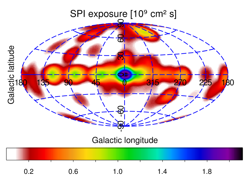
Figure 1: Exposure map of the sky with the SPI telescope on INTEGRAL, for the data used in this analysis (Feb 2003 to Feb 2012).

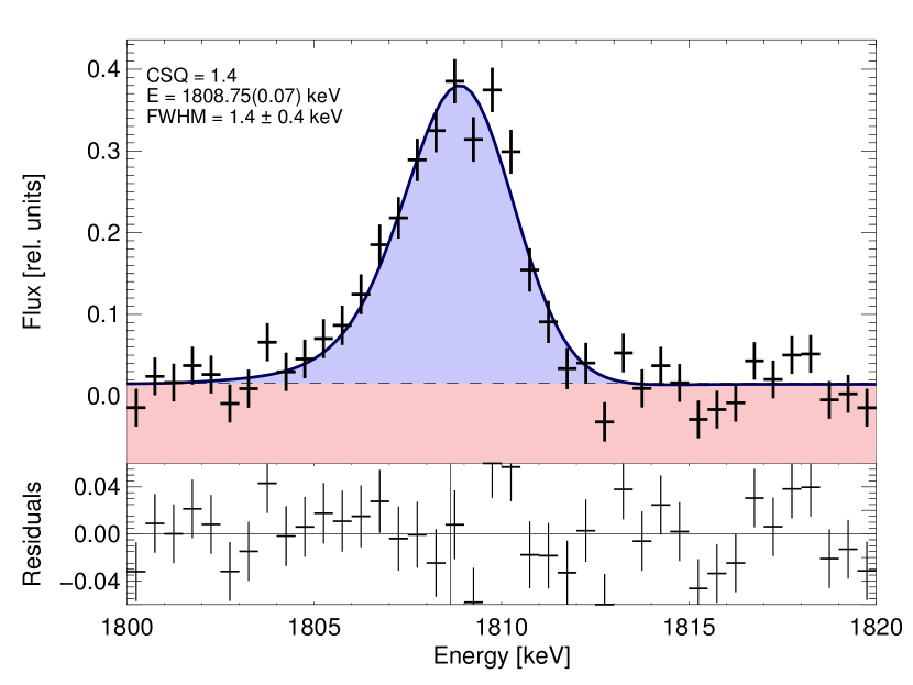
Figure 2: Spectrum around the gamma-ray line from $\@element[26]{\mathrm{Al}}$, as obtained for the entire inner Galactic plane ($\text{ROI}=$128\text{\times}12\text{\,}\mathrm{\SIUnitSymbolDegree}$$ at $l=$$$)

2.2 Generating spectra of celestial emission

Generally, in our spectroscopy analysis we fit the intensity scaling factor of a model of the $\@element[26]{\mathrm{Al}}$ sky intensity distribution plus a scaled model of the instrumental background to the set of spectra accumulated during multi-year observations from our 19 Ge detectors and instrument pointings. Our 9-year observations set includes $65\,302$ instrument pointings that add up to the exposure shown in Fig. 1. Data $d_{k}$ are modelled as a linear combination of the sky model components $M_{ij}$, to which the instrument response matrix $R_{jk}$ is applied, and the background components $B_{jk}$:

$$d_{k}=\sum_{j}R_{jk}\sum_{i=1}^{N_{\mathrm{I}}}\theta_{i}M_{ij}+\sum_{i=N_{\mathrm{I}}+1}^{N_{\mathrm{I}}+N_{\mathrm{B}}}\theta_{i}B_{jk}$$ (1)

i.e. the comparison is performed in data space, which consists of the counts per energy bin measured in each of SPI’s detectors for each single exposure of the complete observation.

By way of the $M_{ij}$ terms, we make use of prior knowledge in the form of a sky intensity distribution such as e.g. the measured $\@element[26]{\mathrm{Al}}$ intensity, or a plausible model such as an exponential disk. We use the $1.8\text{\,}\mathrm{MeV}$ sky map from the COMPTEL gamma-ray telescope (Schoenfelder et al., 1993) on the NASA CGRO mission (1991-2000) (Plüschke et al., 2001) as derived through maximum-entropy deconvolution (Strong, 1995). Our analysis also includes a model for the behaviour of the instrumental background, which is derived from separate analysis of the continuum intensity in energy bands adjacent to the $1808.63\text{\,}\mathrm{keV}$ line and instrumental background tracers in data of the entire INTEGRAL mission. The result of such background study on independent data is a prediction of counts per detector, energy bin, and spacecraft pointing, which is adjusted to the data together with the predicted contribution from the sky (i.e. the sky intensity model as folded into data space using the instrument imaging response function). We then repeat this for $0.5\text{\,}\mathrm{keV}$ wide energy intervals to obtain the sky intensity spectra for such an adopted sky distribution model. In Fig. 2 the spectrum is shown for the entire inner Galaxy, while in Fig. 7, different spectra are shown for spatially separated regions of the sky. The background and sky models and fitting method used in this step are identical to previous work (Wang et al., 2009) and summarised briefly below.

In order to improve in line Doppler shift sensitivity compared to previous SPI results (Diehl et al., 2006), we implemented a new approach for scanning the Galactic plane, employing sky models which are split into two independent components. The sky model we use (e.g. the $\@element[26]{\mathrm{Al}}$ observed with COMPTEL, Plüschke et al., 2001), is divided into two complementary parts: the inside of the spherical rectangle $l\in[l_{0}-\Delta l/2,\ l_{0}+\Delta l/2]$, $b\in[b_{0}-\Delta b/2,\ b_{0}+\Delta b/2]$ defines our region of interest (“ROI”), and its complement with respect to the full-sky map constitutes the second component of the model (Fig. 3). A full-sky model is required, because SPI observation data include events from within the entire telescope field of view of $\sim 30\mathrm{°}$ extent, although the intrinsic spatial resolution of SPI has been determined as $2.7\mathrm{°}$. The sky model thus represents the spatial detail of the fitted intensity within a longitude/latitude bin (ROI); the intensity is fitted to SPI data for the entire ROI; spatial details within ROI bins have little impact on the spectral-line results due to the low total $\@element[26]{\mathrm{Al}}$ signal per ROI. This was confirmed, using different plausible $\@element[26]{\mathrm{Al}}$ sky maps with different structural detail on the scale below $\sim$ few degrees.

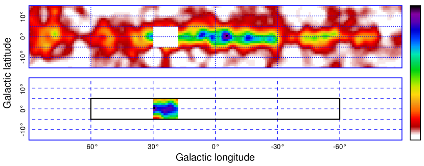
Figure 3: Two sky model components: The region of interest (“ROI”) $12\text{\times}10\text{\,}\mathrm{\SIUnitSymbolDegree}$ centred around $l=$$$ (bottom) and its complement (top), taken as subsets of the COMPTEL $1.8\text{\,}\mathrm{MeV}$ sky map. The rectangular outline shows the region covered by our scan along the Galactic plane.

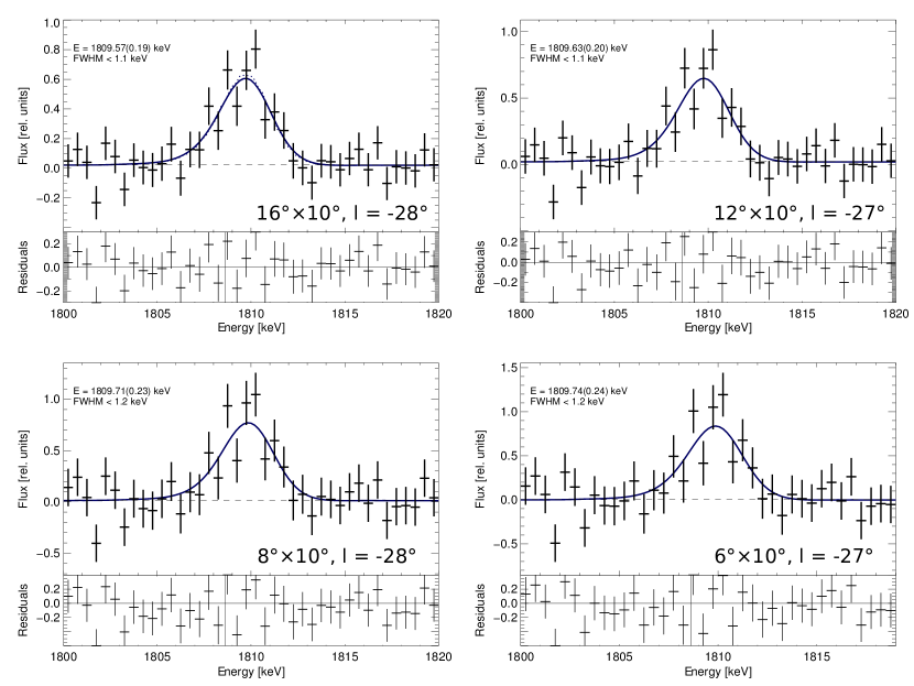
Figure 4: Spectra of the region around $l\sim{}$$-27\text{\,}\mathrm{\SIUnitSymbolDegree}-28\text{\,}\mathrm{\SIUnitSymbolDegree}$ for ROI latitude extents of $16\text{\,}\mathrm{\SIUnitSymbolDegree}12\text{\,}\mathrm{\SIUnitSymbolDegree}8\text{\,}\mathrm{\SIUnitSymbolDegree}6\text{\,}\mathrm{\SIUnitSymbolDegree}$

The intensities of these two components, together with a model of the instrumental background, are then fitted to the SPI data. Our background model reproduces the time variability of the background at short timescales ($<3\text{\,}\mathrm{d}\mathrm{a}\mathrm{y}\mathrm{s}$) with the rate of events saturating the germanium detectors, which has been found to be a sensitive measure of the instantaneous charged particle environment of the instrument. The long term background variation ($>3\text{\,}\mathrm{d}\mathrm{a}\mathrm{y}\mathrm{s}$) is extracted from the continuum intensity in energy intervals adjacent to the $1808.63\text{\,}\mathrm{keV}$ line.

Thus we obtain spectra in the energy range $1800\text{\,}\mathrm{keV}1820\text{\,}\mathrm{keV}$ around the $\@element[26]{\mathrm{Al}}$ line for the two complementary sky model components. We repeat this process, varying $l_{0}$ to scan the ROI along the Galactic plane, and obtain measurements of the $\@element[26]{\mathrm{Al}}$ line signal as a function of Galactic longitude. Fig 4 shows sample results for a particular such region-of-interest in the fourth quadrant of the Galaxy towards longitude $l\sim{}$$-27\text{\,}\mathrm{\SIUnitSymbolDegree}-28\text{\,}\mathrm{\SIUnitSymbolDegree}$ (the centre longitude is not identical because of the $4\text{\,}\mathrm{\SIUnitSymbolDegree}3\text{\,}\mathrm{\SIUnitSymbolDegree}2\text{\,}\mathrm{\SIUnitSymbolDegree}3\text{\,}\mathrm{\SIUnitSymbolDegree}$ rasters – one quarter or one half of the longitude extent – used for the different respective longitude extents).

The latitude range $\Delta b=$$$ in our analysis was chosen to cover the full expected scale height for both ejecta as well as gas streaming away from the plane of the Galaxy towards the halo even for nearby segments of the Galaxy. This is equivalent to $\pm 270\text{\,}\mathrm{pc}$ at $3\text{\,}\mathrm{kpc}$ distance; the CO disk scale height is $\sim 50\text{\,}\mathrm{pc}$ (Dame et al., 2001), a previous $\@element[26]{\mathrm{Al}}$ scale height estimate (Wang et al., 2009) finds a range $\sim 60\text{\,}\mathrm{pc}\sim 250\text{\,}\mathrm{pc}$. But foreground emission, which would predominantly be showing up at intermediate or higher latitudes, may lead to possible biases: The ROI, which corresponds to a pyramid in 3D-space, covers different distances from the Galactic plane, depending on the distance to the emitting region. Nearby sources, taking up a large solid angle on the sky across the plane would thus be sampled only partially, depending on the ROI latitude extent. The influence of the choice of ROI longitude and latitude extent on the model fit results is discussed in greater detail in Appendix A.

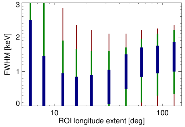
Figure 5: Limits on the width of the $\@element[26]{\mathrm{Al}}$ line emission from ROIs around the Galactic centre with an extent in latitude of $\pm 6\mathrm{°}$ and longitude extents ranging from $6\text{\,}\mathrm{\SIUnitSymbolDegree}128\text{\,}\mathrm{\SIUnitSymbolDegree}$. The error bars of decreasing thickness show the (Bayesian) highest posterior density credible regions corresponding to $68.268\,950\text{\,}\mathrm{\char 37\relax}95.449\,974\text{\,}\mathrm{\char 37\relax}99.730\,020\text{\,}\mathrm{\char 37\relax}$, corresponding to .

The spread of radial velocities over the longitude range covered implies an overall broadening of the line emission when considering the integrated emission coming from a large ROI on the sky. When we vary the extent of the extent of the ROI and with it the range of radial velocities being integrated over, and compare this to the measured line width, we can check the broadening effect of different samples of the sky and its varying kinematic properties. This is shown in Fig. 5, where the error bars show the variation of the measured line width’s confidence intervals with longitude extent. For small regions on the sky, only upper limits on the $\@element[26]{\mathrm{Al}}$ line width can be obtained. The upper limits become smaller with increasing region size as more signal is covered by the region-of-interest before increasing again for $\Delta l\la$$$ as the covered radial velocity range increases. For the large region along the entire inner Galaxy ($128\text{\times}12\text{\,}\mathrm{\SIUnitSymbolDegree}$, Fig. 2), we derive $1.4\pm 0.4\text{\,}\mathrm{keV}$ (FWHM) additional broadening, or $230\pm 70\text{\,}\mathrm{km}\text{\,}{\mathrm{s}}^{-1}$. This is consistent with the spread of radial velocities we measure spatially resolved along the inner Galaxy (Sect. 3.1). The root-mean-square of our radial velocity measurements (Fig. 8), weighted with the corresponding intensity measurements (Fig. 14) is $\approx 200\text{\,}\mathrm{km}\text{\,}{\mathrm{s}}^{-1}$. We thus conclude that observed line broadenings are consistent with systematic variation of line position along the plane of the Galaxy, attributed to large-scale rotation of gas within the Galaxy.

2.3 Characterizing celestial emission lines

In a second step, we fit these spectra of sky intensity values obtained per energy bin and per component by a model description based on the instrument’s spectral response. This yields the $\@element[26]{\mathrm{Al}}$ line parameters of total intensity, Doppler shift with respect to laboratory energy, and intrinsic width of the celestial $\@element[26]{\mathrm{Al}}$ emission, for the respective component of the sky. The spectral model we use in our line fitting consists of a linear continuum and a line at the position $a_{3}$, where the line is the convolution of the instrument spectral response $R$ and a Gaussian $G$ with the width $a_{4}$ ($E_{0}$ is the midpoint of the energy interval):

$$I(E)=a_{0}+a_{1}(E-E_{0})+a_{2}(R*G_{a_{4}})(E-a_{3})$$ (2)

Such detailed modelling of the instrument response is required, as the impact of cosmic radiation onto SPI detectors gradually deteriorates the charge collection properties of detectors, and leads to a degraded spectral response.

The degradation of Ge detectors from cosmic-ray irradiation and its restoration in annealings results in a time variable width and asymmetry of the spectral response. This variation of the spectral response dominates over all other spectral changes, and is found consistent across the SPI energy range. Figure 6 shows how the degradation – as measured by the width of a one-sided exponential tail on the low-energy side of the line response – varies for lines in four different energy regimes. The degradation increases in an approximately linear fashion with time and is reduced periodically by the annealing operations. These heat the detectors for a period of $\sim 2$ weeks to $\sim 100\text{\,}\mathrm{\SIUnitSymbolCelsius}$, restoring the original high spectral resolution. The annealing cycle of one roughly every 6 months (as needed) lead to a sawtooth-like variation of the spectral response during our data taking. Clearly, the absolute magnitude of degradation increases with energy, yet changes occur consistently for all instrumental lines, and are in the range of tenths of $\mathrm{keV}$. Spectroscopic analysis at high precision needs to account for these effects.

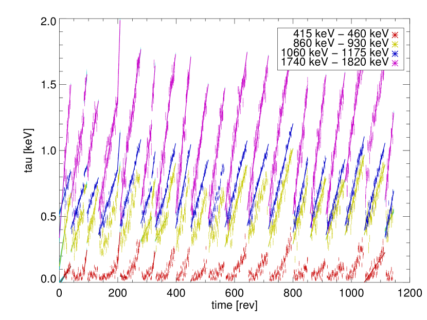
Figure 6: Degradation of the spectral response over mission time. With degradation, a one-sided tail at the low-energy side develops. The plot shows its extent versus time (one revolution = $3\text{\,}\mathrm{d}\mathrm{a}\mathrm{y}\mathrm{s}$).

We estimate the spectral-model parameters (continuum intensity and slope; line intensity, Doppler shift, and width) using the Metropolis-Hastings MCMC algorithm (Neal, 1993), which samples the parameter space statistically to generate detailed probability distributions for the model parameters. This approach allows us to determine accurate limits on the width of the emission line even though the differences between the measured line profiles and the instrumental line response are small. Figure 7 compares the observed Doppler shifts of the $\@element[26]{\mathrm{Al}}$ line to the spectral appearance of a nearby instrumental line for exactly the same data, i.e. all selected SPI pointings around the respective longitude ROI. It is evident that the energy calibration is stable, and the relative changes of the response are small (see Sect. 3.1 below and Fig. 6). The MCMC analysis also determines the Bayes factor (Gelman et al., 2003), i.e. the ratio of the marginal likelihoods of the model including a line and the alternative model that consists of continuum only. If the Bayes factor is larger than one, the model with a line is more probable than the one without, although the line detection may still be insignificant in terms of statistical acceptance criteria. Because of the large numbers involved, it is more convenient to state the Bayes factor on the logarithmic decibel ($\mathrm{dB}$) scale. The longitude-velocity graph (Fig. 8) shows the result of this process for $\Delta l=$$$, $\Delta b=$$$. For our $12\text{\times}10\text{\,}\mathrm{\SIUnitSymbolDegree}$ ROI, the Bayes factor reaches a maximum of $135\text{\,}\mathrm{dB}$, which corresponds to a detection significance of . For the sky distribution model from the $\@element[26]{\mathrm{Al}}$ emission as derived with COMPTEL, and evaluated over the region $|l|<$$$, $|b|<$$$, the Bayes factor and detection significance values are $2100\text{\,}\mathrm{dB}$ and , respectively. Therefore, for sky region sizes as we use here in our ROIs with $\sim 120\text{\,}\mathrm{s}\mathrm{q}\mathrm{u}\mathrm{a}\mathrm{r}\mathrm{e}\mathrm{d}\mathrm{e}\mathrm{g}\mathrm{r}\mathrm{e}\mathrm{e}\mathrm{s}$ or less, the line widths are not tightly constrained, and we give upper limits only; these are: $<1.9\text{\,}\mathrm{keV}$ (i.e. $<315\text{\,}\mathrm{km}\text{\,}{\mathrm{s}}^{-1}$; $95.4\text{\,}\mathrm{\char 37\relax}$, ), or $<2.75\text{\,}\mathrm{keV}$ ($<455\text{\,}\mathrm{km}\text{\,}{\mathrm{s}}^{-1}$; $99.7\text{\,}\mathrm{\char 37\relax}$, ). Only integrating the signal over a larger solid angle allows a more precise line width measurement (Fig. 2 and Sect. 3.1).

The basic instrument spectral response is obtained from the instrumental background line at $1764.494\text{\,}\mathrm{keV}$, which is due to the $\@element[214]{\mathrm{Bi}}$ $\beta$-decay inside SPI’s anticoincidence shield. This response is shown in Fig. 7 (right-hand set of spectra). Its shape is nearly Gaussian, it exhibits however an excess towards the low-energy side that is due to partial charge collection and which varies with the degradation state of the detectors between annealings (Roques et al., 2003), as described above.

For a given ROI position, we determine the spectral response from all exposures where SPI was pointed at a location within a field-of-view radius ($16\mathrm{°}$) around the ROI. We add the spectral responses of the active SPI detectors, we also adjust the absolute energy scale to compensate for the radial velocity due to the Earth’s orbital motion, further adjust the energy scale relative to the line centroid to extrapolate the widening of the instrument energy response with increasing photon energy. We sum these per-exposure spectra, subtract the linear continuum and normalize the result to obtain the SPI energy response for this ROI.

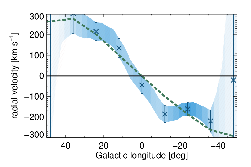
Figure 16: Longitude-velocity results using different methods of determining the spectral response (see Sect. 2.3). For comparison we show: Blue data points and blue shading in the background: measured instrumental background line; red hatched regions in the foreground: line shape model fitted to a set of instrumental background lines.

We also tested a different spectral response determination, which uses a parametrized analytic function (the convolution of a Gaussian with an exponential defined on $x\leq 0$) to describe the line shape, and extracts the line shape parameters from a set of eleven strong instrumental background lines with high time resolution ($3\text{\,}\mathrm{d}\mathrm{a}\mathrm{y}\mathrm{s}$) over the multi-year observation. The impact of the choice of the energy response model on the measured longitude-velocity dependence is negligible, as shown in Fig. 16: The RMS difference for the longitude range $$$\leq l\leq$$$ is $0.15\text{\,}\mathrm{keV}$ ($25\text{\,}\mathrm{km}\text{\,}{\mathrm{s}}^{-1}$), i.e. small by comparison. Appendix A discusses the systematic uncertainties due to the instrumental response modelling in greater detail.

3 Results

3.1 Longitude-velocity diagrams

With the parametrization of the sky along the plane of the Galaxy in bins of different Galactic longitude (at fixed latitude bin width), we obtain spectra near the $\@element[26]{\mathrm{Al}}$ line along the plane of the Galaxy (Fig. 7), as compared to a nearby instrumental background line. The line from decay of $\@element[26]{\mathrm{Al}}$ (laboratory energy $1808.63\text{\,}\mathrm{keV}$) is seen for different regions along the plane of the Galaxy (left), at galactic longitude, $l$, $-24\text{\,}\mathrm{\SIUnitSymbolDegree}24\text{\,}\mathrm{\SIUnitSymbolDegree}$, for a latitude range $\Delta b=\pm$$$ centred at $b=$$$. The shift of the line centroid with galactic longitude is apparent, in particular when compared to an instrumental line nearby (right; line at $1764.494\text{\,}\mathrm{keV}$, from activation of $\@element{\mathrm{Bi}}$ in SPI’s anticoincidence detector made of BGO scintillator; background-line data are selected from the same observations which contribute to the longitude bin shown on the left). The instrumental line at $1764.494\text{\,}\mathrm{keV}$ demonstrates a stable energy calibration for all observations, and in particular absence of a bias with Galactic longitude. The line shape of the instrumental line was used to represent the instrumental spectral response, and used to fit the data in the left-side graphs, thus determining the line position accurately even for weak signals. The systematic shift of the $\@element[26]{\mathrm{Al}}$ line with Galactic longitude can clearly be seen in this subset of spectra, which are selected from non-overlapping, independent sky regions.

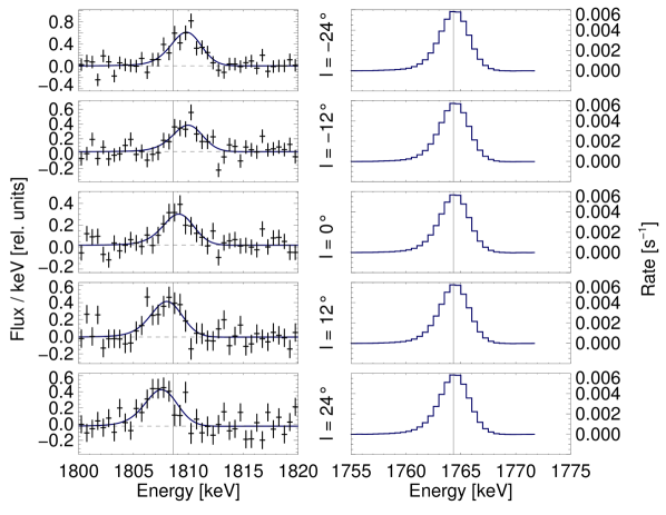
Figure 7: Trace of systematic Doppler shifts of the $\@element[26]{\mathrm{Al}}$ line along the inner Galaxy.

We convert the measured offsets in the centroids of the $\@element[26]{\mathrm{Al}}$ line from the expected $\@element[26]{\mathrm{Al}}$ decay at the laboratory value into the corresponding bulk Doppler velocity. This allows us to construct a longitude-velocity diagram from $\@element[26]{\mathrm{Al}}$ measurements. Figure 8 shows the result, as derived from the spectra shown in Fig. 7. This longitude-velocity result is assembled from the above analysis, which we repeated for the regions-of-interest (ROI) defined by rectangular bins in longitude (widths $6\text{\,}\mathrm{\SIUnitSymbolDegree}8\text{\,}\mathrm{\SIUnitSymbolDegree}12\text{\,}\mathrm{\SIUnitSymbolDegree}16\text{\,}\mathrm{\SIUnitSymbolDegree}$) and latitude (heights $4\text{\,}\mathrm{\SIUnitSymbolDegree}6\text{\,}\mathrm{\SIUnitSymbolDegree}8\text{\,}\mathrm{\SIUnitSymbolDegree}10\text{\,}\mathrm{\SIUnitSymbolDegree}$, Fig. 13). Increasing the ROI size trades spatial resolution against energy resolution. Our choice of a $12\text{\times}10\text{\,}\mathrm{\SIUnitSymbolDegree}$ ROI offers balanced statistical and systematic energy uncertainties (see Appendix A). By moving the ROI in Galactic longitude, we can trace velocities along the plane of the Galaxy. In the figure, we show data points (crosses with error bars showing one standard deviation) spaced $12\mathrm{°}$ apart, i.e. offset by integer multiples of the ROI width and therefore measuring non-overlapping ROIs. We also show (in blue shading) measurements obtained by a closer spaced $3\mathrm{°}$ longitude sampling which implies that neighbouring ROIs overlap by $3\text{/}4$. This oversampling leads to a stronger correlation between neighbouring measurements, but it shows more information than the data points. The blue shaded areas show a colour saturation proportional to the Bayes factor of the spectral model compared to continuum-only, i.e. they show the significance of the signal for each ROI position. The systematic blueshift in the 4^th and redshift in the 1^st Galactic quadrant are expected from large-scale Galactic rotation.

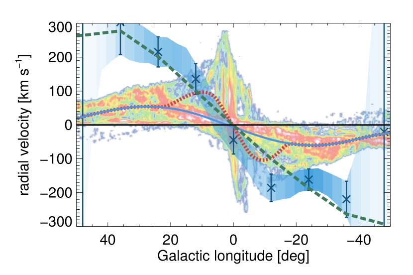
Figure 8: Longitude-velocity diagram comparing $\gamma$-ray-measured velocities (crosses, including error bars) with other objects in our Galaxy. $\@element[26]{\mathrm{Al}}$ line-centroid energies were fitted to determine velocities in longitude bins of $12\text{\,}\mathrm{\SIUnitSymbolDegree}$ and latitude ranges $\pm 5\mathrm{°}$. For comparison, different models are shown (blue solid, red dotted, and green dashed lines), as well as the velocity information from molecular gas as seen in CO (details see Sect. 4).

4 Discussion

Extraction of the spatio-kinematic characteristics of interstellar gas in the inner Galaxy remains a challenge, due to distance ambiguities, observational biases, and the model-dependence of velocity and distance derivations – in addition to the intrinsic differences in resolution of different observables. Our derived line centroids along the Galactic ridge at $l\in[$$,$$]$ (Sect. 3.1) represent the average radial velocities, subject to distance-dependent weighting, of $\@element[26]{\mathrm{Al}}$ in volume slices covering the whole inner Galactic plane. As shown in Fig. 8, we clearly find observed line-of-sight velocities (relative to the local standard of rest) between approximately $200\text{\,}\mathrm{km}\text{\,}{\mathrm{s}}^{-1}$ (redshifted) and $-200\text{\,}\mathrm{km}\text{\,}{\mathrm{s}}^{-1}$ (blueshifted). The excess velocities beyond those globally expected from Galactic rotation are $100\text{\,}\mathrm{km}\text{\,}{\mathrm{s}}^{-1}$ and higher at the velocity maxima, which are near longitudes $\pm$$$.

We believe the most likely explanation for our findings to be the preferential expansion of superbubbles towards the leading edges of spiral arms. This implies a net asymmetry of the million-year-scale bubble expansions that results in a blow-out of massive star ejecta into the low-density region ahead of and outward from the spiral arms. For the kinematic description of $\@element[26]{\mathrm{Al}}$ we must adopt a model for the large-scale spatial distribution and kinematic behaviour of $\@element[26]{\mathrm{Al}}$ as it decays. We now discuss different large-scale kinematic models, which should explain the signature with longitude of $\@element[26]{\mathrm{Al}}$ data points, and finally support our suggested interpretation.

4.1 Spatio-kinematic modelling of the ²⁶Al longitude-velocity signature

4.1.1 Galaxy models with different large-scale rotation components

In Fig. 8, we show in the continuous blue line what the signature from $\@element[26]{\mathrm{Al}}$ would be, if we assume that the density distribution of the $\@element[26]{\mathrm{Al}}$ in the disk and spiral arms of the Galaxy is proportional to large-scale distribution of the free electron density (Cordes & Lazio, 2002), and that the gas is on circular orbits with the velocity given by a Galactic rotation measurement compilation (Sofue et al., 2009). This line shows what our gamma-ray telescope would have measured in longitude-velocity space, while averaging over the same $12\mathrm{°}$ longitude range as used in our data analysis. This is, expectedly, similar to the ridge seen in CO, which is shown in Fig. 8 as colour scale overlay for comparison (from Dame et al., 2001). Clearly, in high-spatial-resolution CO data, additional Galactic features can be resolved, such as the peculiar motions in the nuclear disk close to the centre of the Galaxy. The kinematics of molecular gas displays dominant features along the Galactic ridge, beyond this peculiar motion in the central $\sim$ few $100\text{\,}\mathrm{pc}$ at rather high velocities. But our $\@element[26]{\mathrm{Al}}$ results do not follow these expectations along the Galactic ridge, hence clearly the hot, ejecta-carrying gas does not move as molecular gas does, on these larger scales. Apparently, $\@element[26]{\mathrm{Al}}$ carrying interstellar gas moves at systematically-higher velocities on a large scale than does the CO-traced molecular gas along the ridge of the Galaxy. For longitudes $|l|\ga$$$, its average velocity even exceeds the terminal velocity of CO, the highest radial velocity seen at a given longitude (Englmaier & Gerhard, 1999).

What about the influence of the inner bar in our Galaxy? The dotted red line shows what would be expected if $1\text{/}3$ of the $\@element[26]{\mathrm{Al}}$ was distributed along the Galaxy’s long bar, and $2\text{/}3$ of $\@element[26]{\mathrm{Al}}$ distributed throughout the disk and spiral arms as above. Here, the observed slope of the longitude-velocity signature of $\@element[26]{\mathrm{Al}}$ is reproduced in the inner part, but apparently $\@element[26]{\mathrm{Al}}$ kinematics still is characteristically different outside the regions of the Galaxy’s bar itself, and inner spiral arm regions are involved.

The dashed green line in Fig. 8 combines spiral-arm sources outside a radius $r_{0}$ at large-scale galactic rotation with a new leading-edge blow-out of $\sim 200\text{\,}\mathrm{km}\text{\,}{\mathrm{s}}^{-1}$, which we suggest is an essential part of explaining the $\@element[26]{\mathrm{Al}}$ kinematics. We describe this model and variants in the following subsections. Apparently, a bar-like distribution of sources could reproduce our data only for the inner longitude range, while a model based on two spiral arms extending from the tips of the bar, with large-scale rotation and a leading-edge blow-out at $200\text{\,}\mathrm{km}\text{\,}{\mathrm{s}}^{-1}$, provides a closer match to the data and explains the general longitude-velocity trace as observed in $\@element[26]{\mathrm{Al}}$ gamma-rays.

In the following subsections, we therefore provide more detail on such model variants.

4.1.2 Two-arm spiral models

A simple first-order model to better explain the kinematic properties of the observed $\@element[26]{\mathrm{Al}}$ emission is based on the following assumptions: The spatial distribution of $\@element[26]{\mathrm{Al}}$ in the Galaxy is along a two-arm spiral structure as derived from density wave theory (see below for a four-arm model):

$$\phi=\frac{1}{\tan(i)}\log\left(\frac{r}{r_{0}}\right)\ \text{for galactocentric radii}\ r>r_{0}$$ (3)

where $\phi$ and $i$ denote the azimuth and pitch angle, respectively, and galactocentric radius $r_{0}$ defines the inner end of the spiral arms, which also are assumed to constitute the outer ends of the Galactic bar. The bar itself does not contribute to the emission in this model, it only defines the points where the spiral arms begin. We assume $R_{0}=$8\text{\,}\mathrm{kpc}$$ for the distance of the Sun from the Galactic centre. From observations of stars and gas, the spiral-arm pitch angle has been constrained (Francis & Anderson, 2012) to $5.56\mathrm{°}$. The $\@element[26]{\mathrm{Al}}$ emission is assumed to originate from a $0.5\text{\,}\mathrm{kpc}$ thick layer around the above-defined spiral arms as emission zones (the model results below are not sensitive to reasonable variations of this number), and declines from inner to outer arm regions as a power law in azimuth angle, i.e. $\sim\phi^{a}$. For the intrinsic velocity of $\@element[26]{\mathrm{Al}}$ nuclei at their decay, we adopt an additional azimuthal motion (the blow-out velocity $v_{\mathrm{bo}}$), on top of the rotational velocity, which is adopted as $250\text{\,}\mathrm{km}\text{\,}{\mathrm{s}}^{-1}$ everywhere (Reid et al., 2009, and discussion in Dobbs & Burkert, 2012). Additionally we parametrize the bar angle $\alpha$, i.e. the angle between the line from the Galactic centre to the Sun and the line from the Galactic centre to the near end of the bar, as seen from the Galactic centre: it is taken to be $38\mathrm{°}$, towards the upper end of the range reported by different studies (Francis & Anderson, 2012; Green et al., 2011; Long et al., 2013; Wang et al., 2012; Martinez-Valpuesta & Gerhard, 2011). Smaller bar angles tend to decrease the fit quality and increase the blow out velocity by about $10\text{\,}\mathrm{\char 37\relax}$. Our assumption on the bar angle is consistent with recent measurements from star counts: Wegg & Gerhard (2013) find an angle of $27\pm 2\mathrm{°}$. There is the possibility that the outer bar is twisted (the so-called long bar, see Benjamin et al., 2005; Cabrera-Lavers et al., 2008), e.g. the bar could have leading ends (Martinez-Valpuesta & Gerhard, 2011). The spiral arm ends could be leading the bar even more. In fact, our bar angle is defined by the spiral arm ends and not major axis of the bar. Our model is vertically unresolved as our data are (latitude bin width $10\mathrm{°}$); for comparison, the nearest spiral arm at $\sim 3\text{\,}\mathrm{kpc}$ distance extends over $\sim 1\text{/}2$ of our latitude bin width for an assumed $\@element[26]{\mathrm{Al}}$ scale height of $130\text{\,}\mathrm{pc}$ (Wang et al., 2009).

When we perform a $\chi^{2}$ minimization of this model for our $\@element[26]{\mathrm{Al}}$ longitude-velocity data with free parameters $r_{0}$, $i$, $v_{\mathrm{bo}}$ and $\alpha$, we obtain results as shown in Table 1. This includes fitting or fits adopting $i$ as constant $i=$$$, and two different bar angles $\alpha$.

Table 1: Best-fit parameters for our two-armed spiral emission model with different assumptions about the input parameters. For the main paper, we have adopted the model with fixed $\alpha=$$$ and $i=$$$. The rightmost column shows reduced $\chi^{2}$ as a measure of fit quality. We also include our best-fit four-arm spiral in the bottom row.

Input Parameters		Fitted Parameters
Bar angle	Pitch angle	Bar radius	Pitch angle	$\@element[26]{\mathrm{Al}}$ drop-off	$\@element[26]{\mathrm{Al}}$ vel.	$\chi^{2}$
$\alpha$	$i$	$r_{0}\ [$\mathrm{kpc}$]$	$i$	$a$	$v_{\mathrm{bo}}\ [$\mathrm{km}\text{\,}{\mathrm{s}}^{-1}$]$
$38\mathrm{°}$		$4.4$	$7.7\mathrm{°}$	$0.35$	$220$ p m 60	$1.63$
$38\mathrm{°}$	$5.56\mathrm{°}$	$4.6$		$0.40$	$225$ p m 50	$1.79$
$20\mathrm{°}$	$5.56\mathrm{°}$	$4.9$		$0.65$	$240$ p m 60	$2.00$
$38\mathrm{°}$		$4.1$	$-0.19\mathrm{°}$ / $10.25\mathrm{°}$	$0.01$	$180$ p m 75	$1.01$

We show the relative contributions along each line of sight of the assumed source distribution for the preferred two-arm model (Fig. 9) in Fig. 10. Effectively, the foreground part of the source emission along each line of sight dominates the observed signal. Towards the far bar end, the velocity of the $\@element[26]{\mathrm{Al}}$ carrying gas turns out to be similar to the velocity of gas in the foreground arm. Moreover, the foreground arm dominates in brightness. Hence, the far end of the bar cannot be disentangled.

In summary, the blowout velocity depends only very weakly on changes to any of the parameters of the model. For the results of our paper we have adopted the fit for a fixed $\alpha=$$$ and $i=$$$, and blowout velocity $v_{\mathrm{bo}}=$225\pm 50\text{\,}\mathrm{km}\text{\,}{\mathrm{s}}^{-1}$$, because $\chi^{2}$ is only marginally worse, and for consistency with a recent study (Francis & Anderson, 2012). This model is shown in Fig. 9.

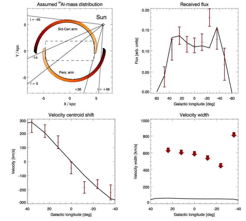
Figure 9: Properties of our preferred model used in the main text. The top left plot shows the adopted $\@element[26]{\mathrm{Al}}$-source distribution in the plane of the Milky Way as seen from above. Also indicated is the position of the Sun ($8\text{\,}\mathrm{kpc}$ from the Galactic centre), the location of the bar (dashed) and several longitudinal directions of interest. The colour indicates the $\@element[26]{\mathrm{Al}}$-density (yellow: highest, black: lowest). The other plots show quantities derived from this source distribution as a function of Galactic longitude as solid black lines (top right: received flux in arbitrary units, bottom left: velocity centroid shift, bottom right: velocity width). Overplotted are the observed data points with 1-standard-deviation-sized error bars, and 3-standard-deviation upper limits in the case of the velocity width. The flux excess at $l=$$$ may be due to foreground emission from the Sco-Cen association (Diehl et al., 2010) leaking from higher latitudes into our ROI bin. The observational limits on the velocity width are not constraining and compatible with expectations (see Sect. 2.2).

4.1.3 Four-arm spiral models

We also investigated four-arm spiral models for the Galaxy, with characteristics similar to the two-arm model. The best-fit four-arm model (Fig. 11) leads to a reduced $\chi^{2}$ of $0.93$, thus formally fits much better than the two-arm model. However, the improved fit quality is mainly due to a better, but still not fully satisfactory match of the flux at $l=$$$, which we believe to be related to foreground emission. We therefore prefer the best-fit two-arm model over the four-arm one, because it has fewer parameters. The inferred blow-out velocity depends weakly on this choice (compare Table 1).

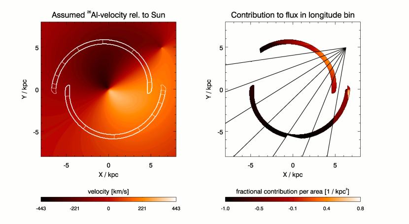
Figure 10: Left: Map of the local velocity relative to the Sun in our preferred model. The white contours indicate the $\@element[26]{\mathrm{Al}}$ mass distribution. Right: Relative flux contribution per surface area in the standard model, separate for each longitude bin. Several longitude bins are indicated by black lines.

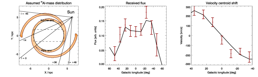
Figure 11: Similar to Fig. 9, but for the best-fit four-arm spiral.

4.2 Comparison to other studies

4.2.1 Spiral arm structure

Confidence levels for two respective pairs of our model parameters are shown in Fig. 12. Clearly, a pitch angle of $5.56\mathrm{°}$ is consistent with our data, within uncertainties. Our favoured Galactic-bar radius falls into the range of published values (Francis & Anderson, 2012; Martinez-Valpuesta & Gerhard, 2011).

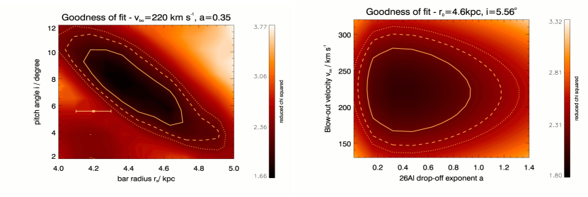
Figure 12: Reduced $\chi^{2}$ and confidence contours as a function of galactocentric bar radius and pitch angle for the Galactic spiral structure (left, the value from Francis & Anderson (2012). is also indicated, including 1-standard-deviation error bars) and as a function of the $\@element[26]{\mathrm{Al}}$-drop-off exponent and the blowout velocity (right). The $68\text{\,}\mathrm{\char 37\relax}90\text{\,}\mathrm{\char 37\relax}95\text{\,}\mathrm{\char 37\relax}$ confidence levels are shown by the solid, dashed and dotted lines. For the left plot, the overall best-fit values of $a=$0.35$$ and $v_{\mathrm{bo}}=$220\text{\,}\mathrm{km}\text{\,}{\mathrm{s}}^{-1}$$ have been kept fixed. For the right plot, the pitch angle from (Francis & Anderson, 2012) $(i=$$)$ and the best-fit bar radius for fixed $i=$$$, $r_{0}=$4.6\text{\,}\mathrm{kpc}$$, has been used (see also Martinez-Valpuesta & Gerhard (2011)). The blowout velocity depends only weakly on these parameters (compare Table 1).

4.2.2 Gas components in our and other galaxies

The blow-out velocity that we derive is inconsistent with velocity variations expected at spiral shocks in the context of simple density wave theory without explicit consideration of the interaction of massive star feedback with the underlying density structure: Our obtained velocities significantly exceed the ones found in molecular (Dame et al., 2001) and atomic gas (Kalberla & Dedes, 2008). Gas-kinematics models (Fux, 1999; Bissantz et al., 2003; Baba et al., 2010; Khoperskov et al., 2013) are in good agreement with these observations, but do also not produce velocities which come close to the ones we find. Shetty et al. (2007) extract the azimuthal velocity variations from CO data for the galaxy M51, which features very prominent spiral arms. Even for the stronger spiral arm in M51, the azimuthal velocity shear does not exceed $\approx 120\text{\,}\mathrm{km}\text{\,}{\mathrm{s}}^{-1}$. The massive stars are however observed downstream of the maximum of the CO intensity, wherefore only a small fraction of the velocity shear would appear as $\@element[26]{\mathrm{Al}}$-velocities in M51. Further, most of the velocity shear in M51 is due to the slowing down of the gas at the spiral shock, such that the azimuthal velocity drops significantly below the circular velocity. Our observations require however velocities of at least $130\text{\,}\mathrm{km}\text{\,}{\mathrm{s}}^{-1}$ (three standard deviations) above the circular velocity. The picture derived by detailed molecular gas observations for M51 (Egusa et al., 2011) would explain our data well: Molecular clouds enter the spiral shock from behind and merge there to larger clouds. This triggers the formation of massive stars downstream of the density maximum. Thus the massive star ejecta are impeded by the upstream density maximum and obtain a net velocity into the direction of rotation.

Our results imply that blow-out occurs from the star-forming regions of the spiral arms within the plane and plausibly also towards the halo. We expect star formation to occur as gas falls into the spiral-arm potential (Wada et al., 2011; Athanassoula, 1992). Observed young star clusters tend to be associated with spiral arms, particularly towards their inner ends and at the near (López-Corredoira et al., 1999) and far (Davies et al., 2012) ends of the Galaxy’s bar. Simulations (Athanassoula, 2012) and face-on images (Elmegreen, 2012) of barred spiral galaxies confirm this general picture. Inside the corotation radius, objects move faster than the large-scale patterns of the bar and of the spiral arms. Consequently, gas clouds which enter the pattern and form stars will create stellar groups that appear offset towards the leading edge of the pattern. For the Galactic bar, a corotation radius of $\sim 4\text{\,}\mathrm{kpc}$ has been found (Gerhard, 2011), though estimates increase to $5\text{\,}\mathrm{kpc}6\text{\,}\mathrm{kpc}$ if both a boxy bulge and bar are considered (Martinez-Valpuesta & Gerhard, 2011). A corotation of $\sim 8.4\text{\,}\mathrm{kpc}$ has been found for the spiral arms of our Galaxy (Lépine et al., 2011). For a pattern velocity difference of $\sim 50\text{\,}\mathrm{km}\text{\,}{\mathrm{s}}^{-1}$, an offset of $\sim 200\text{\,}\mathrm{pc}$ between superbubble-blowing massive stars and spiral-arm density maximum would be expected at the end of a typical massive-star lifetime of $\sim$ few ${10}^{6}\text{\,}\mathrm{y}\mathrm{e}\mathrm{a}\mathrm{r}\mathrm{s}$. The $\@element[26]{\mathrm{Al}}$ sources typically located in a density gradient on one side of the large-scale density enhancement in arms would trace non-isotropic superbubble growth around massive star groups, which otherwise cannot easily be seen in remains from parental molecular clouds (Louie et al., 2013). Although systematic velocity variation across spiral arms is expected from density wave theory and has been found in M51 (Shetty et al., 2007), such velocity differences across a spiral arm are only $\sim 100\text{\,}\mathrm{km}\text{\,}{\mathrm{s}}^{-1}$ or lower, and cannot explain our measurement (see Sect. 4.1). Simulations show that the initially isotropic ejecta from massive stars face and enhance the high-pressure region on one side, and a champagne-like outflow into the opposite direction occurs within a rather short time (Fierlinger et al., 2012; Baumgartner & Breitschwerdt, 2009). Our observations require that $\@element[26]{\mathrm{Al}}$-enriched superbubbles preferentially expand in the direction of galactic rotation relatively unimpeded, whereas they are blocked by denser gas in the opposite direction. This probably occurs along spiral arms and near the tip of the bar where the two prominent inner spiral arms curve towards the bar. Interestingly, velocities around $200\text{\,}\mathrm{km}\text{\,}{\mathrm{s}}^{-1}$ are close to the sound speed in the hot gas (${10}^{6}\text{\,}\mathrm{K}$). von Glasow et al. (2013) model the absorption systems seen at similar velocities against Lyman break galaxies as cooled-down shells from expanding superbubbles. In both cases, the velocity would be set by the sound speed of the hot phase the superbubbles are expanding into.

4.2.3 Hot gas in and above the Galactic plane

Similar velocities perpendicular to the Galactic plane are also consistent with the scale height of $\@element[26]{\mathrm{Al}}$ measured (Wang et al., 2009) as $130^{+120}_{-70}$ $\mathrm{pc}$: The characteristic scale height of parental molecular clouds is about $50\text{\,}\mathrm{pc}$ (Dame et al., 2001), while, for example, a velocity of $200\text{\,}\mathrm{km}\text{\,}{\mathrm{s}}^{-1}$ implies that a height of about $200\text{\,}\mathrm{pc}$ above the parental clouds is reached within the decay time of ${10}^{6}\text{\,}\mathrm{y}\mathrm{e}\mathrm{a}\mathrm{r}\mathrm{s}$. Such velocities cannot support a wind from the Galaxy into the intergalactic medium. Since $\@element[26]{\mathrm{Al}}$ traces superbubbles with ongoing input by massive stars, these should exhibit the highest velocities, whereas older bubbles that are not highlighted by $\@element[26]{\mathrm{Al}}$ will be less dynamic. Hot gas at higher latitudes above the Galactic disk is also seen in O vi absorption (Sembach et al., 2003). Such high ionization states appear in hot and relatively dense gas, as the superbubble wall interacts with ambient gas. O vi data reflect more closely the average hot gas in general, including the later stages of superbubble evolution: the observed O vi height is $2\text{\,}\mathrm{kpc}3\text{\,}\mathrm{kpc}$ (Sembach et al., 2003).

Within the Galactic disk, the velocities inferred from absorption also do not directly follow the molecular gas velocities, but are closer (Sembach et al., 2003) to them than to the higher velocities we infer for $\@element[26]{\mathrm{Al}}$. Therefore, asymmetries that we observe during the active superbubble phase apparently are dissipated, and the flow is more isotropic at later times.

5 Conclusions

Our measurements of the Doppler shifts of the $1808.63\text{\,}\mathrm{keV}$ line as a function of Galactic longitude show that the radial velocity of the interstellar gas containing $\@element[26]{\mathrm{Al}}$ in the inner Galaxy differs significantly from that of other components of the ISM such as those seen in CO or H I. We observe the same qualitative behaviour: there is almost no average radial motion in the direction toward the the Galactic centre, the magnitude of the radial velocity increases with the angular separation from the centre up to $|l|\sim$$$ and the sign of the radial velocity is positive (redshift) in the first and negative (blueshift) in the fourth Galactic quadrant. However, the absolute velocities of the $\@element[26]{\mathrm{Al}}$-carrying gas are much larger. Since the line emission happens over a large radial velocity range, the total emission from the inner Galaxy is Doppler-broadened. Our measurements of the line width of the $\@element[26]{\mathrm{Al}}$ emission are compatible with this implication. The variation of our measured radial velocity values with the extent of the region-of-interest we average over is comparable to the statistical uncertainties and the systematic uncertainties related to the time dependent variation of the instrument’s spectral response are small in comparison. Since the majority of $\@element[26]{\mathrm{Al}}$ is produced in massive stars, we conclude that our observations are probably due to large-scale asymmetric outflows from the regions where massive stars have formed recently.

The inner spiral arms, which are the plausible source regions producing most of the $\@element[26]{\mathrm{Al}}$, show blow-out of their massive-star ejecta preferentially into the direction of the leading edges. This increases $\@element[26]{\mathrm{Al}}$ velocities to $\sim 200\text{\,}\mathrm{km}\text{\,}{\mathrm{s}}^{-1}$ in addition to large-scale galactic rotation. Superbubbles are expected to form around massive star groups on the $\mathrm{Ma}$ time scale (Krause et al., 2013). In a wind-blown cavity or supernova remnant, initially freely-travelling ejecta would be decelerated within a time much shorter than a radioactive-decay lifetime. The $\@element[26]{\mathrm{Al}}$-rich ejecta accumulate behind the swept up ambient medium, expanding at a similar velocity. When estimating the line-of-sight averaged velocities of $\@element[26]{\mathrm{Al}}$ as it decays, we should distinguish between the velocity of the bubble expansion itself and the velocities of ejecta flows within a bubble. Bubbles from single stars are expected to reach sizes on the order of $10\text{\,}\mathrm{pc}$ with associated expansion velocities of order $10\text{\,}\mathrm{km}\text{\,}{\mathrm{s}}^{-1}$. Our inferred expansion velocity of $\sim 200\text{\,}\mathrm{km}\text{\,}{\mathrm{s}}^{-1}$ shows that the bubbles highlighted by $\@element[26]{\mathrm{Al}}$ have to be powered by many, hence clustered, massive stars. While we defer detailed consistency checks via cluster-population synthesis to future work, our measurement together with the fact that $\@element[26]{\mathrm{Al}}$ ejection is strongly correlated to the energy injection (Voss et al., 2009) suggests that massive star feedback in the inner few $\mathrm{kpc}$ of the Galaxy and its spiral arms is dominated by sizeable star clusters producing superbubbles, constituting a fundamental unit of large-scale stellar feedback. This does not imply expansion of the superbubble as an entity with such velocities, but rather provides a measurement from its interior reflecting its size and position with respect to the $\@element[26]{\mathrm{Al}}$ sources.

Our measurements reveal new aspects of large-scale gas kinematics in the Galaxy, derived from data originating in the hot and tenuous phase of the ISM that is otherwise hard to measure. Flow asymmetries require distinct structure within the spiral arms of the Galaxy: dense gas, which marks the spiral-arm potential, must be offset upstream from massive stars, and these must be located towards the spiral-arm leading edges, with ejecta blowing out into the inter-arm low density environment (and halo). Origins of spiral arms are debated (Wada et al., 2011), and massive star offsets from their gas density maxima remain controversial (Louie et al., 2013; Ferreras et al., 2012). The excess velocity of $\@element[26]{\mathrm{Al}}$-traced gas over stars and cold/dense gas (Fig. 8) thus constitutes a clear, though indirect, demonstration of the offsets between star-forming gas and young stars, which seemed plausible in density-wave theory and have also been found in molecular gas observations (Vogel et al., 1988) and images of galaxies (Elmegreen, 2012) (see also Sect. 4.1).

This one sided blow-out will impart a local braking torque on the cold gas as it rotates in the plane of the Galaxy. Once injected into the halo, hot gas will likely exchange its angular momentum with the ${10}^{6}\text{\,}\mathrm{K}$ corona (Gupta et al., 2012) over $\sim{10}^{8}\text{\,}\mathrm{a}$ before cooling and returning to the Galactic disk elsewhere (Marinacci et al., 2011). The total mass of $\@element[26]{\mathrm{Al}}$ in the Milky Way is measured (Diehl et al., 2006) to be $\sim 2\text{\,}\mathrm{M_{\sun}}$. This traces about ${10}^{6}\text{\,}\mathrm{M_{\sun}}$ of total massive-star ejecta, hence a hot gas flow of $\sim 1\text{\,}\mathrm{M_{\sun}}\text{\,}{\mathrm{a}}^{-1}$, ejected into the direction of Galactic rotation, with an excess velocity comparable to the Galactic rotation velocity itself. These $\@element[26]{\mathrm{Al}}$ data measure primarily a torque of a specific, and otherwise hard to observe, gas component, which also couples to the total of Galactic gas flows. The global recoil may slow down denser gas in its rotation in the Galaxy: Its global torque of $$1\text{\,}\mathrm{M_{\sun}}\text{\,}{\mathrm{a}}^{-1}$\cdot$4\text{\,}\mathrm{kpc}$\cdot$200\text{\,}\mathrm{km}\text{\,}{\mathrm{s}}^{-1}$\approx${10}^{6}\text{\,}\mathrm{M_{\sun}}\text{\,}{\mathrm{kpc}}^{2}\text{\,}{\mathrm{Ma}}^{-2}$$ can be compared to the total angular momentum of the Milky Way’s gas of roughly $${10}^{10}\text{\,}\mathrm{M_{\sun}}$\cdot$5\text{\,}\mathrm{kpc}$\cdot$250\text{\,}\mathrm{km}\text{\,}{\mathrm{s}}^{-1}$\approx${10}^{10}\text{\,}\mathrm{M_{\sun}}\text{\,}{\mathrm{kpc}}^{2}\text{\,}{\mathrm{Ma}}^{-1}$$. To estimate potential impacts, this blow-out could remove the entire angular momentum from the dense gas within $10\text{\,}\mathrm{Ga}$. This estimate assumes that the angular momentum would not return to the disk. More realistically, some angular momentum exchange with the gaseous halo will take place, and some fraction of the angular momentum will return to the disk when the ejecta fall back. Estimated radial inflow rates toward the inner Galaxy for other processes are (Crocker, 2012) $0.1\text{\,}\mathrm{M_{\sun}}\text{\,}{\mathrm{a}}^{-1}1\text{\,}\mathrm{M_{\sun}}\text{\,}{\mathrm{a}}^{-1}$ due to gravitational or $0.2\text{\,}\mathrm{M_{\sun}}\text{\,}{\mathrm{a}}^{-1}$ due to magnetic torque, and $0.2\text{\,}\mathrm{M_{\sun}}\text{\,}{\mathrm{a}}^{-1}$ by mass loss from the bulge stars. Radial gas diffusion is implied by one-sided superbubble blowout even if there was no global loss of angular momentum from the Galactic disk, because it would require substantial fine-tuning of the angular momentum-exchange between the off-streaming $\@element[26]{\mathrm{Al}}$-traced gas and the halo gas to get the $\@element[26]{\mathrm{Al}}$-traced gas back to its original position. One-sided superbubble blow-out may thus contribute both to linking general star formation on $\mathrm{kpc}$ scales to large-scale gas flows and to subsequent star formation in the inner regions of our Galaxy. Our measured characteristic ejecta velocity suggest that superbubbles are the dominant structure of the ISM around massive stars.

The UV luminosity associated with massive stars is important in ionizing gas at higher Galactic latitudes and towards the halo (Razoumov & Sommer-Larsen, 2006): It’s propagation and escape from the denser parts of the disk depends critically on the structure of the interstellar medium around its sources and the erosion of spiral-arm gas around massive stars. The morphology of surrounding interstellar gas determines the extent to which UV from massive stars may reach more distant gas, and contributes to the ionization state of the intergalactic medium. Blow-out from massive star regions in superbubbles is thus a fundamental aspect of large-scale stellar feedback in a star-forming galaxy such as our own. This effect must be accounted for in models (Veilleux et al., 2005) of galactic winds and galaxy evolution, which currently consider either single, non-interacting bubbles, or the galaxy as a whole with simplified structural assumptions at scales below $\sim$ $\mathrm{kpc}$ scales.

Appendix A Systematic uncertainties

We investigated the impact of choosing sky region bins of different sizes, e.g. smaller at the expense of a smaller signal, but aiming to obtain a better spatial resolution for our velocity information (spectra in Fig. 4 illustrate this specifically towards longitude $l\sim{}$$-27\text{\,}\mathrm{\SIUnitSymbolDegree}-28\text{\,}\mathrm{\SIUnitSymbolDegree}$, the brightest part of the 4^th Galactic quadrant). Figure 13 shows the dependence of the $\@element[26]{\mathrm{Al}}$ velocity results on the ROI extent in longitude (varying between $6\mathrm{°}$ and $16\mathrm{°}$), and in latitude (between $6\mathrm{°}$ and $10\mathrm{°}$). We can obtain higher spatial resolution, but only in regions of high intensity. In our longitude-velocity figures, we include the Bayes factor information for $B>1$ also for the data points where detections are insignificant, and the data point values therefore are not shown themselves in the figure. In order to maximize the $\@element[26]{\mathrm{Al}}$ signal for best determination of its line centroid position, we chose a latitude range of $\pm 5\mathrm{°}$ for our definite analysis.

The variation of intensity (per solid angle, averaged over the ROI) with latitude extent offers some indication that the intensity falloff with latitude is slower in the inner ($|l|<$$$) Galactic plane. Figure 14 shows these intensity variations for latitude extents of $6\text{\,}\mathrm{\SIUnitSymbolDegree}8\text{\,}\mathrm{\SIUnitSymbolDegree}10\text{\,}\mathrm{\SIUnitSymbolDegree}$ as well as the difference between $10\mathrm{°}$ and $6\mathrm{°}$ ROIs as “high latitude” (units are relative). We can see that the intensity distribution varies consistently for different latitude integration regions of $6\text{\,}\mathrm{\SIUnitSymbolDegree}10\text{\,}\mathrm{\SIUnitSymbolDegree}$, except for a possible additional component between longitudes $+5\mathrm{°}$ and $-12\mathrm{°}$. This component may arise from the Scorpius-Centaurus region (Diehl et al. 2010). This different behaviour in the inner Galaxy also is seen in the shape of the $\@element[26]{\mathrm{Al}}$ line: It appears that we see a superposition in the region $l\sim[$$,$$]$ (see Fig. 14) of a nearby (and more extended in latitude) component which is approximately at rest with respect to the observer, and the Doppler-shifted component from the Galactic plane. Therefore, the line shape is less well represented by a single Gaussian, and the uncertainties in centroid determination are larger in this inner region of the Galactic plane (see Fig. 13). (Additionally, in $l\sim[$$,$$]$ the line is less bright than at $|l|\sim[$$,$$]$, further increasing the line centroid’s uncertainty).

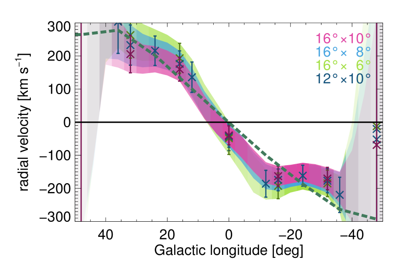
Figure 13: $\@element[26]{\mathrm{Al}}$ longitude-velocity results for different bin sizes in Galactic longitude (above) and latitude (below).

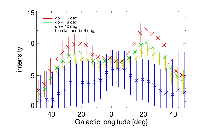
Figure 14: $\@element[26]{\mathrm{Al}}$ intensities along the inner Galaxy, for different bin sizes in Galactic latitude, and $16\mathrm{°}$ bins in longitude, offset in $4\mathrm{°}$ steps. The emission which can be attributed to higher latitudes, hence potential foreground sources, is indicated in the lowest (blue) data points, derived from the difference in intensities for the $6\mathrm{°}$ and $10\mathrm{°}$ bins.

Detailed tracking of the spectral response variation with degradations and annealings has been found necessary for determining the width of the $\@element[26]{\mathrm{Al}}$ line (as shown in Fig. 2). But the effect of the spectral response variation on the line position measurements for smaller emission regions is small: compare Fig. 2 to Fig. 7). For example, with an instrumental line width of $3\text{\,}\mathrm{keV}$ and a celestial line width of $1.4\text{\,}\mathrm{keV}$ (Fig. 2), the measured width is $\sqrt{($3\text{\,}\mathrm{keV}$)^{2}+($1.4\text{\,}\mathrm{keV}$)^{2}}\approx$3.31\text{\,}\mathrm{keV}$$, which is a $10\text{\,}\mathrm{\char 37\relax}$ excess above the instrumental width.

Figure 15: Offset in line centroids from the effect of time-variable degradation, if a line with fixed centroid would be represented by a Gaussian fit. Periods where the respective longitude range was observed are used, so that the impact on our longitude-velocity result can directly be seen.

We then investigated this variation for a correlation with the times of our observations along the plane of the Galaxy, possibly leading to a longitude-dependent bias. For this, we determine the maximum position shift in units of velocity, measured by when fitting an instrumental line to the data that were taken while pointing at the respective longitude intervals. As shown in Fig. 15, the bias which may result from this time-variable spectral response is small ($<10\text{\,}\mathrm{km}\text{\,}{\mathrm{s}}^{-1}$) compared to our reported line-shift values.

The observed velocity values for different latitude ranges are all consistent within the uncertainties.

We conclude that the systematic uncertainties in our longitude-velocity measurement are smaller than statistical uncertainties and do not alter the results reported, specifically the asymmetry of blow-out as discussed. Also our background method and spectral-response treatment does not have an impact on the results. Systematics are dominated by the selection of the ROI used, and may affect the detailed velocity value derived for a particular region along the Galactic plane by $\sim 50\text{\,}\mathrm{km}\text{\,}{\mathrm{s}}^{-1}$.