An Analytical Model of Packet Collisions
in IEEE 802.15.4 Wireless Networks

Abstract

Numerous studies have shown that concurrent transmissions can help to boost wireless network performance despite the possibility of packet collisions. However, while these works provide empirical evidence that concurrent transmissions may be received reliably, existing signal capture models only partially explain the root causes of this phenomenon. We present a comprehensive mathematical model for MSK-modulated signals that makes the reasons explicit and thus provides fundamental insights on the key parameters governing the successful reception of colliding transmissions. A major contribution is the closed-form derivation of the receiver bit decision variable for an arbitrary number of colliding signals and constellations of power ratios, time offsets, and carrier phase offsets. We systematically explore the factors for successful packet delivery under concurrent transmissions across the whole parameter space of the model. We confirm the capture threshold behavior observed in previous studies but also reveal new insights relevant to the design of optimal protocols: We identify capture zones depending not only on the signal power ratio but also on time and phase offsets.

0.8[0.5,0.5](0.5,0.94)  

This is the accepted version of the article (with additional figures), to appear in IEEE Transactions on Wireless Communications.
For the final version visit http://dx.doi.org/10.1109/TWC.2014.2349896 once it becomes available. © 2014 IEEE. Personal use of this material is permitted. Permission from IEEE must be obtained for all other uses, in any current or future media, including reprinting/republishing this material for advertising or promotional purposes, creating new collective works, for resale or redistribution to servers or lists, or reuse of any copyrighted component of this work in other works.

I Introduction

Conventional wireless communication systems consider packet collisions as problematic and try to avoid them by using techniques like carrier sense, channel reservations (virtual carrier sense, RTS/CTS handshakes), or arbitrated medium access (TDMA, polling). The intuition is that concurrent transmissions cause irreparable bit errors at the receiver and render packet transmissions undecodable. However, researchers have found that this notion is too conservative. If the power of the signal of interest exceeds the sum of interference from colliding packets by a certain threshold, packets can in general still be received successfully despite collisions at the receiver. This effect, referred to as the capture effect [1], has been explored extensively and validated in many independent practical studies on various communication systems such as IEEE 802.11 [2, 3, 4, 5] and IEEE 802.15.4 [6, 7, 8].

Over the past years, the view on packet collisions has therefore changed considerably. Since it is possible for some or even all packets in a collision to survive, there are opportunities to increase the overall channel utilization and to improve the network throughput by designing protocols that carefully select terminals for transmitting at the same time [9, 10]. The benefits and potential performance improvements of concurrent transmission are not just of theoretical interest but have been demonstrated practically and adopted in application areas such as any-cast [11, 12], neighbor counting [13], or rapid network flooding [14, 15, 16, 17, 18], especially in the context of wireless sensor networks (WSNs).

Although protocols that exploit concurrent transmissions have shown the potential to boost the overall performance of existing wireless communication systems, their success cannot be explained with capture threshold models based on the Signal to Interference and Noise Ratio (SINR) alone. Recent studies have shown that, while the relative signal powers of colliding packets indeed play an important role in the reception probability, other factors are also of major importance. For example, several experimental studies report that the relative timing between colliding packets has a significant influence on the reception probability [5, 19]. Others report that the coding [20] or packet content [11] may also greatly influence the reception performance in the presence of collisions. Further factors such as the carrier phase offset between a packet of interest and colliding packets also need to be considered [21].

In this paper, we strive to provide a comprehensive model accounting for all these factors, focusing on packet collisions in IEEE 802.15.4 based WSNs. Such a model will allow protocol designers to better understand the root causes of packet reception and exact conditions under which concurrent transmissions actually work, and thus to design optimal protocols based on these factors. While previous studies [3, 7, 22, 23, 24] also looked at factors that determine the success of concurrent packet reception, these works are either based on practical experiments and have therefore led to empirical models that cannot be generalized easily, or derived simplified models that do not account for all impact factors. This work advances the field by providing a unified analytical model accounting for the major factors identified above (see also II). Our model ($\rightarrow$ III) is based on a mathematical representation of the physical layer using continuous-time expressions of the IQ signals entering the receiver’s radio interface. This fundamental and comprehensive model allows to represent an arbitrary number of colliding packets as a linear superposition of the incoming signals.

A major contribution of this work is a closed-form analytical representation of the bit decision variable at an optimal receiver’s demodulator output based on these IQ signals ($\rightarrow$ IV). This result enables the deterministic computation of the bit demodulation decision and hence to compute the actual performance of concurrent transmissions for any colliding parameter constellations. Having a bit-level model of reception is not only beneficial for the comprehension of the collision process, it also contributes to application areas where a precise bit-level analysis is needed, such as partial packet reception [25], understanding bit error patterns in low-power wireless networks [26, 27], or signal manipulation attacks at the physical layer [21].

Using our model, we explore the parameter space of the reception of MSK-modulated colliding packets considering both uncoded and Direct Sequence Spread Spectrum (DSSS) based systems ($\rightarrow$ V), analyzing the influence of the parameters on the resulting packet reception ratio (PRR) for concurrent transmissions. While the analysis shows that our model agrees with experimental results in the literature, it also provides much more detailed insights into the performance characteristics of protocols that exploit collisions [14, 11, 15, 16, 17, 18]. In particular, we show that the good performance of these protocols should be attributed equally to coding (e.g., DSSS) and power capture. In addition, based on our analysis we identified parameter constellations where concurrent transmissions work reliably. We therefore propose a generalization of the traditional capture threshold model based on the power ratios towards a capture zone. Capture zones result from the model insight that reception success does not depend on the power ratio between interfering signals alone, but on the time and phase offsets of sender and receiver as well.

To show the validity and accuracy of our model, we implemented and experimented with an application that is strongly dependent on physical layer characteristics, the reception of unsynchronized signals. We performed this experiment with two widely used commercial IEEE 802.15.4 receiver implementations (TI CC2420 and Atmel AT86RF230) to demonstrate that our results are receiver-independent ($\rightarrow$ VI). The results validate our claim that our model accurately captures the behavior of realistic receivers in the face of concurrent transmissions. Finally, we discuss parameter settings for an optimal protocol design ($\rightarrow$ VII).

II Impact Factors

Different factors influence the probability of a successful reception under collisions. This section discusses the main factors that have been identified in the literature. Subsequently, we consider them jointly in our mathematical model to predict the outcome of concurrent transmissions.

Power ratio

The signal power is a crucial factor for successful reception in general, and it plays a major role in the reception under collisions as well. SINR-based models are widely used to model the packet reception in a shared medium, for example in the Physical Model [28] and its variants [29, 30]. The classical SINR model states that a stronger signal is received if its signal power $P_{s}$ exceeds the channel noise $P_{n}$ and the sum of interfering signal powers $\sum_{i}P_{i}$ by a given threshold, i.e.,

$$\frac{P_{s}}{P_{n}+\sum_{i}P_{i}}>\delta_{\mathrm{SINR}}.$$

This simple model is accurate for uncorrelated interfering signals such as additive white Gaussian noise (AWGN). However, when the interference is correlated (such as colliding packets), this model is not always accurate and further factors must be considered [3, 5, 19].

Signal timing

The relative timing of colliding packets greatly influences the reception process. This is because the receiver locks onto a packet during the synchronization phase at the start of the transmission. If a stronger signal arrives later, it captures the receiver and disturbs the first packet reception, and both packets in the collision are lost. Thus, in packet radios, power capture alone is not sufficient for successful reception, rather the receiver must be synchronized and locked onto the captured signal as well. Several research contributions analyze possible collision constellations and their effect on packet reception [5, 19], and propose a new receiver design that releases the lock when a stronger packet arrives, discards the first and receives the second packet, the so-called message-in-message (MIM) capture [5, 22]. Subsequent works apply these insights to improve network throughput. For example, Manweiler et al. [31] propose collision scheduling to ensure that MIM is leveraged, thus increasing spatial reuse.

Channel coding

A further factor that influences packet reception success is bit-level coding. For example, in DSSS systems a group of $b$ bits is encoded into a longer sequence of $B$ chips [32]. The benefit of this approach is that resilience to interference is increased because the chipping sequences can be cross-correlated at the receiver, which effectively filters out uncoded noise. However, DSSS systems require interfering signals to be uncorrelated, e.g., signals without coding or with orthogonal chipping sequences (as in CDMA), to achieve their theoretical coding gain. Another possibility is a sufficient time offset between interfering packets with the same coding; this phenomenon is known as delay capture [20]. As networking standards such as IEEE 802.11 and IEEE 802.15.4 generally use DSSS with identical codes for all participants, existing experimental works on collisions and capture observe the effects of DSSS implicitly.

Packet contents

Experimental results show that packets with identical payload and aligned starting times result in good reception performance and reduced latency in broadcast scenarios. For example, Dutta et al. [11] show that short packets can be received in such collisions with a PRR over 90 %, thus enabling the design of an efficient receiver-initiated link layer. Similarly, the latency of flooding protocols widely used in WSNs can be greatly reduced [15, 17]. In these works, experiments in IEEE 802.15.4 networks reveal that the tolerable time offset between concurrent messages is small (approx. 500 ns), which adds challenges to protocol design and implementation. These insights also show that capture and packet synchronization alone are not sufficient to explain the performance of these protocols, and bit-level modeling that also includes signal timing and content is necessary.

Carrier phase

Considering the reception of bits at the physical layer, knowledge of the carrier phase at the receiver is crucial for successful reception of phase modulated signals because the information is carried in the phase variations of the signal, such that these offsets should be minimized [32]. Typically this is achieved during the synchronization phase of packet reception, and thus existing capture models have omitted phase offsets. However, there are two reasons why this is not sufficient. First, in novel protocols exploiting packet collisions, the synchronization during the preamble is not always able to succeed. Second, there are other new applications of concurrent transmissions that try to abandon the synchronization procedure. For example, Pöpper et al. [21] investigate the possibility of manipulating individual message bits on the physical layer, and conclude that carrier phase offsets are the major hindrance to do so reliably.

III System Model

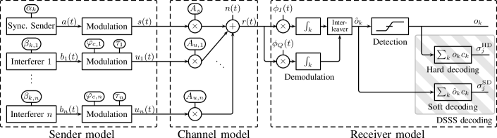
Figure 1: System model, its parameters are shown in ovals (information bits $\alpha_{k},\beta_{k}$, carrier phase offset $\varphi_{c}$, time offset $\tau$, signal amplitudes $A_{s},A_{u}$). We consider one synchronized sender and $n$ interferers on a collision channel that is the input to a receiver. Here, three channel coding schemes are considered, (i) uncoded, (ii) DSSS with hard decision decoding (HDD), and (iii) DSSS with soft decision decoding (SDD); resulting in different receiver paths.

In this section, we discuss the system model underlying our analysis, as shown in 1. It considers all factors from the previous section. From a bird’s eye view, the model consists of three components: (i) the sender model that modulates the physical layer signals of $n+1$ transmitters, one fully synchronized signal of interest (SoI) and $n$ interferers with possibly differing transmission starting times and payloads; (ii) the channel model with all senders sharing a single collision channel that outputs a scaled superposition of all signals (according to their corresponding power at the receiver), and (iii) the receiver model with three detection methods: uncoded, DSSS with hard decision decoding (HDD), and DSSS with soft decision decoding (SDD). In the following, we discuss each component in detail. The notation used is collected in I.

Symbol Definition $s(t)$ MSK signal by the synchronized sender as defined in (LABEL:MSKsig) $u_{i}(t)$ MSK signal by interferer $i$, with possible offsets $\tau_{i}$ and $\varphi_{c,i}$ ((LABEL:ui)) $r\left(t\right)$ Resulting superposition of signals at the receiver ((LABEL:r)) $2T$ Bit duration, e.g., $2T=$1\text{\,}\mathrm{\SIUnitSymbolMicro s}$$ in IEEE 802.15.4 $\omega_{c}=2\pi f_{c}$ Angular speed of the carrier wave with frequency $f_{c}$ $\omega_{p}=\frac{\pi}{2T}$ Angular speed of baseband pulses (periodic by $4T$) $\tau_{i}$ Time offset (positive shifts denote a starting delay) $\varphi_{c,i}$ Carrier phase offset in the passband of interferer $i$ $\varphi_{p,i}=\omega_{p}\tau_{i}$ Baseband pulse phase offset of interferer $i$, equivalent to time offset $A_{s,}A_{u_{i}}$ Signal amplitudes of $s\left(t\right)$, $u_{i}\left(t\right)$ at the receiver $\Pi\left(t\right)$ Unit pulse (step) function as defined in (LABEL:Pulse) $a_{I},a_{Q}\left(t\right)$; $b_{I,}b_{Q}\left(t\right)$ Information sequences consisting of unit pulses $\Pi(t)$ ((LABEL:aIpulse)) $\alpha_{k}^{I},\alpha_{k}^{Q}$; $\beta_{k}^{I},\beta_{k}^{Q}$ Information bit $k$ of the synchronized sender and interferers $\phi_{I},\phi_{Q}\left(t\right)$ Basis function of the MSK modulation to demodulate bits $\Lambda_{u}\left(k\right)$ Contribution of signal $u\left(t\right)$ to the bit decision in bit interval $k$ ((LABEL:Lambda)) $\hat{o}_{k}^{I}$ Decision variable of the detector for bit $k$ of $I$ component $o_{k}^{I}$ Detected bit of an uncoded transmission $\xi$ Input symbol at the sender $c_{\xi,k}$ Chipping sequence of symbol $\xi$ (see also III) $\sigma_{j}^{HD},\sigma_{j}^{SD}$ Detected symbol after DSSS decoding, the index $j$   compensates that each symbol consists of 16 IQ pairs (see (LABEL:DSSSCorr)) $k^{\prime}=k-\left\lfloor\tau/2T\right\rfloor$ Correction factor for the bits active in a decision interval $\underline{\tau}=\tau-2k^{\prime}T$ Relative shift in a bit of interest $k$ $k^{Q\prime}=k-\left\lfloor\left(\tau+T\right)/2T\right\rfloor$ Correction factor for Q bits during I detection $k^{I\prime}=k-\left\lfloor\left(\tau-T\right)/2T\right\rfloor$ Correction factor for I bits during Q detection $\underline{\tau^{Q}}=\tau+T-2k^{Q\prime}T$ Relative shift in a bit of interest $k$ for the leaking Q-phase $\underline{\tau^{I}}=\tau-T-2k^{I\prime}T$ Relative shift in a bit of interest $k$ for the leaking I-phase

Table I: Notation used in the derivations.

III-A Sender Model

In the first component, we modulate the physical signals of $n+1$ senders. We instantiate our model with the Minimum Shift Keying (MSK) modulation, a widely used digital modulation with desirable properties, and of special interest because of its use in the 2.4 GHz PHY of IEEE 802.15.4 [33, $\S$6.5], but we also discuss other modulation schemes including O-QPSK, QPSK, and BPSK. For the signal representations, we follow the notation of Proakis and Salehi [32, $\S$4.3].

III-A1 Synchronized sender

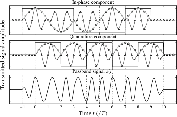
Figure 2: MSK modulation example. The modulated bit sequence is 1110010011 (quadrature-phase bits are shown in boldface); it is multiplexed to the IQ components (blue rectangular pulse trains), pulse-shaped with half-sines (red sinusoids with $\circ$ markers) and modulated on a carrier, resulting in the green waveform (with $\bigtriangleup$ markers). For the quadrature component, we observe an additional staggering of $T$ (MSK can be viewed as Offset-QPSK with half-sine pulse shaping). Both modulated IQ signals are added to result in the (real-valued) passband time signal in the bottom figure.

We assume that the receiver is fully synchronized to the SoI, i.e., the synchronization process has successfully acquired this signal and all interferers have relative offsets to it. The signal is then given by

$$s\left(t\right)=a_{I}\left(t\right)\cos\left(\frac{\pi t}{2T}\right)\cos\omega_{c}t+a_{Q}\left(t\right)\sin\left(\frac{\pi t}{2T}\right)\sin\omega_{c}t.$$ (5)

The signal consists of two components, the in- (I) and the quadrature-phase (Q) components. Modulated onto each component are the information signals (carrying the bits represented by $\alpha_{k}^{I},\alpha_{k}^{Q}\in\left\{\pm 1\right\}$) given by

$$a_{I}\left(t\right)= \sum_{k=-\infty}^{\infty}\alpha_{k}^{I}\Pi\left(\frac{t-2kT}{2T}\right)$$ (6)

$$a_{Q}\left(t\right)= \sum_{k=-\infty}^{\infty}\alpha_{k}^{Q}\Pi\left(\frac{t-\left(2k+1\right)T}{2T}\right),$$ (7)

which represents a train of unit pulses $\Pi$ with duration $2T$, the bit duration of the modulation (e.g., $2T=1$ $\mu$s in IEEE 802.15.4). The unit pulses are defined by

$$\Pi\left(t\right)=\begin{cases}0&\mbox{if }\left|t\right|>\frac{1}{2}\\ \frac{1}{2}&\mbox{if }\left|t\right|=\frac{1}{2}\\ 1&\mbox{if }\left|t\right|<\frac{1}{2}\end{cases}$$ (8)

The information signals are staggered, i.e., the Q-phase information signal is delayed by $T$ in $a_{Q}\left(t\right)$. These signals are then shaped with half-sine pulses of duration $2T$, and modulated onto a carrier with frequency $\omega_{c}/2\pi$ (e.g., 2.4–2.48 GHz in IEEE 802.15.4). In the following, we use the angular frequency of baseband pulses $\omega_{p}=\pi/2T$, such that the first cosine term in Eq. (5) may be represented by $\cos\omega_{p}t$. A graphical illustration of such an MSK-modulated signal is shown in 2.

III-A2 (Unsynchronized) interferers

In addition to the synchronized sender, we consider $n$ interferers transmitting concurrently, using the same modulation. These signals may not be synchronized to the receiver and each may carry its own payload. This introduces three additional parameters that influence the signal, the time offset $\tau_{i}$, the carrier phase offset $\varphi_{c,i}$, and the information bits $\beta_{k,i}$. With a positive $\tau_{i}$, an interfering signal arrives later at the receiver than the synchronized signal. The signal at the receiver for interferer $i$ is given by

$$u_{i}\left(t;\tau_{i},\varphi_{c,i}\right)= \,b_{I,i}\left(t-\tau_{i}\right)\cos\omega_{p}\left(t-\tau_{i}\right)\cos\left(\omega_{c}t+\varphi_{c,i}\right)$$

$$+b_{Q,i}\left(t-\tau_{i}\right)\sin\omega_{p}\left(t-\tau_{i}\right)\sin\left(\omega_{c}t+\varphi_{c,i}\right).$$ (9)

We assume that the phase offsets $\varphi_{c,i}$ are constant for the duration of a packet, i.e., there is no carrier frequency offset during a transmission. In our experiments in VI, we show that this assumption is reasonable because receiver implementations are compensating for possible drifts. For convenience, we express the pulse phase offset caused by $\tau_{i}$ as $\varphi_{p,i}=\omega_{p}\tau_{i}$.

III-A3 Other modulation schemes

While our results are derived for the MSK modulation, it is possible to adapt them to other variants of the phase shift keying (PSK) modulation. We briefly describe the differences to major variants and highlight how these affect the analysis. Further details on the relationship between PSK modulation schemes can be found in Proakis and Salehi [32] and Pasupathy [34].

Offset QPSK

O-QPSK with a half-sine pulse shape is identical to MSK [35] and the results therefore also apply for this modulation. If O-QPSK is used in combination with rectangular pulse shaping instead, the signal is then given by

$$s_{\mathrm{O-QPSK}}\left(t\right)=\frac{1}{\sqrt{2}}\left(a_{I}\left(t\right)\cos\omega_{c}t+a_{Q}\left(t\right)\sin\omega_{c}t\right).$$

The altered pulse shape leads to the omission of the factor $\cos\omega_{p}t$ present in Eq. (5), because the rectangular shaping is already included in the information signal $a\left(t\right)$. This leads to a simplification of our MSK results because pulse phase offsets $\varphi_{p}$ that are caused by the time offset $\tau$ are not present.

Quadrature PSK

Considering QPSK, the change from O-QPSK is the missing time shift $T$ in the quadrature phase. This leads to a different information signal for the Q phase,

$$a_{Q}^{\prime}\left(t\right)=\sum_{k=-\infty}^{\infty}\alpha_{k}^{Q}\Pi\left(\frac{t-2kT}{2T}\right).$$

When adapting our results to QPSK, this affects the indices $k$ of the colliding bits.

Binary PSK

This scheme considers only the in-phase components of QPSK, its signal is given by

$$s_{\mathrm{BPSK}}\left(t\right)=\frac{1}{\sqrt{2}}a_{I}\left(t\right)\cos\omega_{c}t.$$

This simplifies the derivations and results further, because there is no contribution from the Q phase signal in collisions.

III-B Channel Model

In our model, we use an additive collision channel. The relation for the output signal is

$$r\left(t\right)=A_{s}\,s\left(t\right)+\sum_{i=1}^{n}A_{u,i}\,u_{i}\left(t;\tau_{i},\varphi_{c,i}\right)+n\left(t\right).$$ (10)

Each signal is scaled by a positive, real-valued factor $A$, which contains both, possible signal amplifications by the sender and path loss effects that reduce the power at the receiver. In our evaluation, we use the Signal to Interference Ratio (SIR) at the receiver, given by $\mathrm{SIR}=A_{s}^{2}/\left(\sum_{i=1}^{n}A_{u,i}^{2}\right)$, to characterize the power relationship of the interfering signals. The contribution of all noise effects is accumulated in the linear noise term $n\left(t\right)$; possible instantiations are a noiseless channel or a white Gaussian noise channel.

III-C Receiver Model

In the final component of the model, we feed the signals’ superposition $r\left(t\right)$ into an optimal receiver to discern the detected bits. The signal is demodulated and fed into one of three detector implementations: one for uncoded bits, and two variants of DSSS decoding.

III-C1 Demodulation

Demodulation is performed for I and Q individually and the bits are then interleaved. We limit our discussion to the I component for brevity.

We use the matched filter function $\phi_{I}\left(t\right)=\left(2/T\right)\cos\omega_{p}t\cos\omega_{c}t$ and low-pass filtering for downconversion and demodulation, which is the optimal receiver for noiseless and Gaussian channels in the sense that it minimizes the bit error probability [32, §4.3]. The received signal $r\left(t\right)$ is multiplied by $\phi_{I}\left(t\right)$ and integrated for each bit period $k$ to form the decision variable

$$\hat{o}_{k}^{I}=\Lambda_{r}^{I}\left(k\right)=\int_{\left(2k-1\right)T}^{\left(2k+1\right)T}r\left(t\right)\phi_{I}\left(t\right)dt.$$ (11)

The resulting (real) value is called soft bit. Because the combination of the interferers in the received signal is linear, the individual contributions can be divided into integrals for each signal:

$$\hat{o}_{k}^{I}=\Lambda_{s}^{I}\left(k\right)+\sum_{i=1}^{n}\Lambda_{u_{i}}^{I}\left(k\right)+\Lambda_{n}^{I}\left(k\right).$$

In our analytical evaluation in the following section, we derive closed-form expressions for $\Lambda_{u_{i}}^{I}$ and $\Lambda_{u_{i}}^{Q}$ to analyze the receiver output after a signal collision.

We point out that this simplified model does not include receiver-side techniques such as Automatic Gain Control (AGC) or phase tracking; however, we conjecture that the reception performance is still comparable. In fact, as our experiments in VI show, this assumption is justified and the simplified model is able to predict the reception behavior of real-world receiver implementations with good accuracy. We leave the investigation on the effects of these advanced techniques to future work.

III-C2 Uncoded bit detection

The detection operation for uncoded transmissions is slicing, essentially a sign operation on the demodulation output, which results in binary output $o_{k}\in\left\{\pm 1\right\}$. Thus, a bit of the SoI is flipped if the contribution of the interferers changes the bit’s sign.

III-C3 DSSS decoding

For coded transmissions, the number of chips exceeds the bits in a symbol, i.e., even if several chips are flipped it is still possible to decode a symbol correctly. We consider $2^{b}$ symbols $\xi$ with chipping sequence $c_{\xi}$, each with a block length of $B$ bit (i.e., the number of chips). For example, we have $b=4$, $B=32$ in IEEE 802.15.4.

We differentiate two modes of operation for the DSSS decoder, namely hard decision decoding (HDD) and soft decision decoding (SDD) [32].

Hard decision decoding

In HDD, the decoder uses sliced (binary) values $o_{k}$ as its input, and then chooses the symbol with the highest bit-wise cross-correlation of all chipping sequences. In this way, HDD can be viewed as an additional step that takes a group of uncoded bits with $B$ elements (from the uncoded bit detection described above) to determine a symbol $\sigma_{j}^{\mathrm{HD}}$, i.e., a group of $b$ bits. For HDD, the decoder is given by

$$\sigma_{j}^{\mathrm{HD}}=\arg\max_{0\leq\xi<2^{b}}\left|\sum_{k=0}^{B-1}o_{jB+k}\>c_{\xi,k}\right|.$$ (12)

Soft decision decoding

In SDD, the real-valued, unquantized demodulator output $\hat{o}_{k}$ (soft bits) is used as decoder input directly, in contrast to the binary values $o_{k}$ used in HDD. This is beneficial because soft bits provide a measure of detection confidence and demodulation quality, and thus adds weighting to the bits used in the cross-correlation.

IV Mathematical Analysis

No offsets $\Lambda_{u}^{I}\left(k\right)=A_{u}\beta_{k}^{I}$ (1) Carrier phase offset $\varphi_{c}$ $\Lambda_{u}^{I}\left(k\right)=A_{u}\left(\cos\varphi_{c}\beta_{k}^{I}-\frac{1}{\pi}\sin\varphi_{c}\left(\beta_{k-1}^{Q}-\beta_{k}^{Q}\right)\right)$ (2) Time offset $\tau$ $\Lambda_{u}^{I}\left(k\right)=\frac{1}{2T}A_{u}\left(\cos\varphi_{p}\left(\underline{\tau}\beta_{k-1}^{I}+\left(2T-\underline{\tau}\right)\beta_{k}^{I}\right)-\frac{2T}{\pi}\sin\varphi_{p}\left(\beta_{k-1}^{I}-\beta_{k}^{I}\right)\right)$ (3) Carrier phase + time offset $\Lambda_{u}^{I}\left(k\right)=\frac{1}{2T}A_{u}\left\{\cos\varphi_{c}\left(\cos\varphi_{p}\left(\underline{\tau}\beta_{k-1}^{I}+\left(2T-\underline{\tau}\right)\beta_{k}^{I}\right)-\frac{2T}{\pi}\sin\varphi_{p}\left(\beta_{k-1}^{I}-\beta_{k}^{I}\right)\right)\right.$ (4) $\hphantom{\Lambda_{u}^{I}\left(k\right).=iA_{u}\,}\left.-\sin\varphi_{c}\left(\sin\varphi_{p}\left(\underline{\tau^{Q}}\beta_{k^{Q\prime}-1}^{Q}+\left(2T-\underline{\tau^{Q}}\right)\beta_{k^{Q\prime}}^{Q}\right)+\frac{2T}{\pi}\cos\varphi_{p}\left(\beta_{k^{Q\prime}-1}^{Q}-\beta_{k^{Q\prime}}^{Q}\right)\right)\right\}$

Table II: Analytical results: contributions of an interfering signal to the demodulator output $\Lambda_{u}^{I}$ for the $k$-th bit. The results present the relationship between in- and quadrature phase bits sent by an interferer ($\beta^{I}$ and $\beta^{Q}$) with time-adjusted bit indices $k^{\prime},k^{Q\prime}$; it also considers the effects of carrier phase offsets $\varphi_{c}$ and time offsets ($\varphi_{p}$ and $\tau$). The corresponding notation is introduced in Sections III and IV.

Based on the system model in 1, we analyze the contributions of each interfering signal to the overall demodulator output; the sum of these contributions is the decision variable of bit detection. We first present the general case considering all system parameters in 1. Subsequently, we illustrate its interpretation using selected parameter combinations.

Theorem 1.

For an interfering MSK signal $u\left(t\right)$ with offset parameters $\tau$ and $\varphi_{c}$, the contribution to the demodulation output $\Lambda_{u}^{I}\left(k\right)$ is given by Eq. (4) in II.

The proof of this theorem can be found in B. To provide a better understanding of the effects of the parameters, we focus on selected parameter constellations and discuss the resulting equations. Then we revisit 1 and discuss the combination of effects.

IV-1 Synchronized signal

In the simplest case both offsets, time and phase, are zero, i.e., the interfering signal is also fully synchronized to the receiver. The result is given in Eq. (1) in II. The signal’s contribution to the $k$-th bit is $\Lambda_{u}^{I}\left(k\right)=A_{u}\beta_{k}^{I}$. The bit decision of bit $k$, i.e., the sign of the equation, is governed by $\beta_{k}^{I}$. The magnitude of the contribution is controlled by the amplitude of the signal $A_{u}$, and thus stronger signals lead to a greater contribution to the decision variable $\hat{o}_{k}$. As an example, consider two signals $s\left(t\right)$ and $u\left(t\right)$ that are both fully synchronized to the receiver. The detector output of bit $k$ is then $A_{s}\alpha_{k}^{I}+A_{u}\beta_{k}^{I}$. If both senders transmit the same bit ($\alpha_{k}^{I}=\beta_{k}^{I}$), then the signals interfere constructively and push the decision variable further away from zero. If, on the other hand, the bits are different, then the decision variable has the sign of the stronger signal; this is the well-known power capture effect for a single bit.

Figure 3: Carrier phase offset $\varphi_{c}$: several bits influence the bit decision on bit $k$ in a collision between two signals. The carrier phase offsets lead to a leakage of the quadrature phase, and because the Q-bits are staggered, there is an additional shift of $T$ in the bit indices. The active bits in the decision interval are highlighted.

IV-2 Carrier phase offset

Next, we analyze the effect of carrier phase offsets when the signals are fully time-synchronized ($\tau=0$), as shown in 3. The result is given in Eq. (2). We observe two effects of the carrier phase offset. First, the bit contribution of $\beta_{k}^{I}$ is scaled by $\cos\varphi_{c}\leq 1$, which leads to reduced absolute values (and thus a smaller contribution to the decision variable) and potentially causes the bit $\beta_{k}^{I}$ to flip for $\varphi_{c}\in\left(\frac{\pi}{2},\frac{3\pi}{2}\right)$. Second, the quadrature phase starts to leak into the decision variable and thus two additional bits $\beta_{k-1}^{Q},\beta_{k}^{Q}$ influence the outcome. This contribution, however, is scaled by $\pi^{-1}\sin\varphi_{c}$, and only appears when the two Q bits are alternating during the integration interval. In essence, uncontrolled carrier phase offsets may lead to unpredictable bits in the detector output because of carrier phase offset induced bit flips.

Figure 4: Example of a time offset $\tau$ during detection: three bits influence the bit decision on the second bit in a collision between two signals. The active bits in the decision interval are highlighted (the synchronized sender’s bit $\alpha_{1}^{I}$ and interferer’s in-phase bits $\beta_{0}^{I}$ and $\beta_{1}^{I}$).

IV-3 Time offset

If the signals are phase-matched but shifted in time, the detector output is given by Eq. (3). We make three observations here. The bit index $k$ needs to be adjusted because bits may be time-shifted into the integration interval, see 4; the new index is given by $k^{\prime}=k-\left\lfloor\tau/2T\right\rfloor$, with $\left\lfloor\cdot\right\rfloor$ denoting the floor function. We call these active bits because they contribute to the bit decision. These bits overlap partially or fully, and their active time duration is $\underline{\tau}=\tau-2\left\lfloor\tau/2T\right\rfloor T$, the underscore signifies that its value is confined to the interval $\left[0;2T\right)$. However, these bits do not contribute to the decision directly but are scaled by $\cos\varphi_{p}$, which is caused by the half-sine pulse shaping of MSK. This scaling means that bit contributions are diminished and may be flipped by certain time offsets. Finally, a term scaled by $\pi^{-1}$ is introduced that is only present when bits are alternating. However, these bits are the same in-phase bits $\beta_{k-1}^{I},\beta_{k}^{I}$, the Q phase does not leak in this setting.

IV-4 Both offsets

Figure 5: Example of time and phase offsets combined: the decision on the second bit ($k=1$) is influenced by four bits in this example (the synchronized sender’s bit $\alpha_{1}^{I}$, the interferer’s in-phase bits $\beta_{0}^{I}$ and $\beta_{1}^{I}$ due to time shifts, and quadrature bit $\beta_{0}^{Q}$ from carrier phase offsets).

Finally, when both offsets are present as in 1, we can interpret the result as a combination of the above effects. A graphical illustration of the active bits is shown in 5. Due to the staggering of bits (the Q bits are delayed by $T$), the indices of leaking bits of the Q phase also need to be adjusted, the new index is $k^{Q\prime}=k-\left\lfloor\left(\tau+T\right)/2T\right\rfloor$, and the active time interval $\underline{\tau^{Q}}$ is derived similarly to above.

In summary, we observe that the contribution of the interfering signal is complex and that $\varphi_{c}$ and $\varphi_{p}$ can potentially flip the original bits $\beta_{k}^{I}$. This should be bad news for collision-aware protocols that use identical payload to achieve constructive interference (e.g., SCIF [17]): these bits can flip easily and then generate destructive interference. However, coding helps to alleviate these negative effects as we will see in the next section.

V Parameter Space Exploration

Equipped with the closed-form analytical model of the bit-wise receiver outputs, we systematically explore the parameter space of the reception of concurrent transmissions in detail.

V-A Methodology

Symbol $\xi$	Bits	Chipping sequence bits ($c_{\xi,0},\ldots,c_{\xi,31}$)
0	0000	1	1	0	1	1	0	0	1	1	1	0	0	0	0	1	1	0	1	0	1	0	0	1	0	0	0	1	0	1	1	1	0
1	0001	1	1	1	0	1	1	0	1	1	0	0	1	1	1	0	0	0	0	1	1	0	1	0	1	0	0	1	0	0	0	1	0
2	0010	0	0	1	0	1	1	1	0	1	1	0	1	1	0	0	1	1	1	0	0	0	0	1	1	0	1	0	1	0	0	1	0
3	0011	0	0	1	0	0	0	1	0	1	1	1	0	1	1	0	1	1	0	0	1	1	1	0	0	0	0	1	1	0	1	0	1
4	0100	0	1	0	1	0	0	1	0	0	0	1	0	1	1	1	0	1	1	0	1	1	0	0	1	1	1	0	0	0	0	1	1
5	0101	0	0	1	1	0	1	0	1	0	0	1	0	0	0	1	0	1	1	1	0	1	1	0	1	1	0	0	1	1	1	0	0
6	0110	1	1	0	0	0	0	1	1	0	1	0	1	0	0	1	0	0	0	1	0	1	1	1	0	1	1	0	1	1	0	0	1
7	0111	1	0	0	1	1	1	0	0	0	0	1	1	0	1	0	1	0	0	1	0	0	0	1	0	1	1	1	0	1	1	0	1
c8	1000	1	0	0	0	1	1	0	0	1	0	0	1	0	1	1	0	0	0	0	0	0	1	1	1	0	1	1	1	1	0	1	1
9	1001	1	0	1	1	1	0	0	0	1	1	0	0	1	0	0	1	0	1	1	0	0	0	0	0	0	1	1	1	0	1	1	1
10	1010	0	1	1	1	1	0	1	1	1	0	0	0	1	1	0	0	1	0	0	1	0	1	1	0	0	0	0	0	0	1	1	1
11	1011	0	1	1	1	0	1	1	1	1	0	1	1	1	0	0	0	1	1	0	0	1	0	0	1	0	1	1	0	0	0	0	0
12	1100	0	0	0	0	0	1	1	1	0	1	1	1	1	0	1	1	1	0	0	0	1	1	0	0	1	0	0	1	0	1	1	0
13	1101	0	1	1	0	0	0	0	0	0	1	1	1	0	1	1	1	1	0	1	1	1	0	0	0	1	1	0	0	1	0	0	1
14	1110	1	0	0	1	0	1	1	0	0	0	0	0	0	1	1	1	0	1	1	1	1	0	1	1	1	0	0	0	1	1	0	0
15	1111	1	1	0	0	1	0	0	1	0	1	1	0	0	0	0	0	0	1	1	1	0	1	1	1	1	0	1	1	1	0	0	0

Table III: Chipping sequences used in the 2.4 GHz PHY of IEEE 802.15.4.

In order to numerically study the transmission reception success under interference we perform so-called Monte Carlo simulations (see Jain [36]); that means we do time-static simulations of independent packet transmissions in which we randomly vary the analytical model’s parameters to investigate their influence on performance parameters such as packet reception ratio, bit and symbol error rate. Conceptually, the simulator is just a software version of the mathematical model (written in Python) applied to a whole packet; it is not meant to validate the model but to experiment with randomly chosen values for the model parameters and to provide more insights on the success probability of concurrent transmissions. The simulation code is available for download at http://disco.cs.uni-kl.de/content/collisions; there, the interested reader can also find an interactive visualization of the model.

For most experiments, the time offset between sender and interferer is fixed and is our primary factor in the numerical analysis, i.e., in the plots we show the reception performance depending on the time offset. The other parameters of the model are treated as secondary factors and are randomly varied. Generating 1,000 independent packet transmissions for each data point in the presented graphs thus represents the secondary factors’ average contribution to the reception success. We provide more details on the choices for the model’s parameters for sender and channel in the following.

V-A1 Sender model

For ease of presentation, we mainly consider the presence of one synchronized sender and one interferer; we denote these parties as $\mathcal{S}$ and $\mathcal{I}$ with signals $s\left(t\right)$ and $u\left(t\right)$, respectively. In V-B3, we consider the $n$ interferer case separately. We analyze the reception performance of groups of associated bits, or packets; in this case, a single bit error leads to a packet drop. The packet reception ratio (PRR) is the fraction of packets that arrive without errors divided by the total number of packets. We use packets with a length of 64 bit. We consider two categories of colliding packets, either with independent ($\mathcal{S}$ and $\mathcal{I}$ trying to exploit spatial reuse) or identical content ($\alpha_{k}=\beta_{k}$, as it is the case for collision-aware flooding protocols). The bits to send are chosen in the following manner: for uncoded transmissions, $\alpha_{k}$ is drawn bitwise i.i.d. from a Bernoulli distribution over $\left\{-1,1\right\}$, and either the same procedure is performed for $\beta_{k}$ (independent packets) or simply copied over from $\alpha_{k}$ (identical packets). For coded packets, we draw symbols i.i.d. uniform random from $\left\{0,\ldots,15\right\}$ and spread these symbols according to the chipping sequences defined by the IEEE 802.15.4 standard [33, $\S$6.5]. This means that 4 bit groups are first spread to 32 bit chipping sequences before they are transmitted in $\alpha_{k},\beta_{k}$. The chipping sequences are given in III. Note that for symbols 1–7, the chipping sequences are shifted versions of the symbol 0, while for the other half (symbols 8–15), the quadrature-phase bits are inverted.

In accordance to the literature [37], as the carrier phase offset is hard to control because of oscillators drifts and other phase changes during transmission, we draw $\varphi_{c}$ i.i.d. uniform randomly from $\left[0;2\pi\right)$ for each packet unless stated otherwise. On the other hand, we use the same time offset $\tau$ for all packets because experimental work shows that this timing can be precisely controlled. For example, Glossy [15] achieves a timing precision of 500 ns over 8 hops with 96 % probability, and Wang et al. [18] report a 95 % percentile time synchronization error of at most 250 ns. For our simulations, we used 1,000 packets for each value of $\tau$.

V-A2 Channel model

To concentrate on the impact of signal interference, we consider a noiseless channel. This is a well-accepted assumption when both signals are significantly above noise floor level [38, $\S$8]. We set $A_{s}=1$ and $A_{u}=\mathrm{SIR}^{-\frac{1}{2}}$.

V-B Reception of the Synchronized Signal of Interest

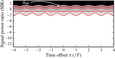
(a) Uncoded transmissions.

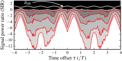
(b) DSSS with hard decision decoding.

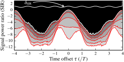
(c) DSSS with soft decision decoding.

Figure 6: The capture threshold for two colliding packets with independent payload, varying with the signals’ power ratio SIR and time offset ($\tau=0$ indicates that the signals overlap fully). For the uncoded case, the threshold $\delta_{\mathrm{SIR}}$ is nearly constant across all time offsets and represents the classical capture threshold (thus, for reference, it is drawn in all figures). For HDD, the threshold is nearly constant, but 1 dB lower. Additionally, there is a wide transitional region with non-zero PRRs. Finally, for SDD the threshold is very sensitive to signal timing, we observe a variation of 6–8 dB with periodical time shifts of $2T$.

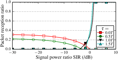
(a) Uncoded transmissions.

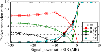
(b) DSSS with hard decision decoding (HDD).

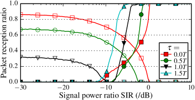
(c) DSSS with soft decision decoding (SDD).

Figure 7: Effect of signal to interference ratio SIR on the PRR for independent payload. Filled markers represent the reception of the synchronized sender’s packets, empty markers represent the reception of the interferer’s packets. (a) For uncoded transmissions and in the negative SIR regime, the reception of the interferer’s packets is poor (max. 30 % PRR) even with perfect time synchronization ($\tau=0$). The synchronized sender requires a positive SIR for a high PRR independent of the interferers timing, and the transitional region is narrow. (b) For HDD, the interferer’s packets have an increasing chance of reception, strongly depending on the timing. For the synchronized sender, the transitional region is widened. (c) This behavior is even more pronounced for the SDD case, with a PRR of the interferer of over 85 % and the SIR transitional zone has a width of 10 dB.

V-B1 Capture threshold under independent payload

In our first case study, we consider the transmission of independent payload. This situation occurs, e.g., when two uncoordinated senders detect a clear channel, transmit, and the packets collide at the receiver. Our metric of interest is the PRR of the SoI, i.e., we observe the probability to overcome the collision. The results for three classes of receivers are shown in 6 and 7.

Uncoded transmissions. From 6a, we observe that the capture threshold is a good model to describe the PRR of interfering, uncoded transmissions. If the SoI is stronger by a threshold $\delta_{\mathrm{SIR}}$ of 2 dB, all its packets are received. This behavior persists for all choices of $\tau$, i.e., packet reception is independent from the properties of the interfering signal (we only see a minor periodic effect). Below the threshold, there is a narrow transitional region with non-zero PRR. Under uncoded transmissions, our model is able to recover the classical capture threshold for MSK and is in accordance to experimental results in the literature [6, 8].

Hard decision decoding. When considering HDD (6b), we note that the threshold abstraction is still valid and the performance improvement of coding is only 1 dB (the coding gain is canceled when the same chipping sequences are used). In the transitional region, there is a wider parameter range that results in non-zero PRRs, e.g., when $\tau$ is close to integer values (and thus $\cos\varphi_{p}\approx 0$), we observe a better PRR for $\mathcal{S}$. These results show that coding with HDD yields only limited benefits if all senders use identical chipping sequences.

Soft decision decoding. Finally, for SDD we observe a strong dependence between PRR and time offset (6c). Only for positions without chipping sequence shifts ($\tau=0$, and because of the way IEEE 802.15.4 sequences are chosen, $\tau=4kT$, $k\in\mathbb{Z}$) the performance is comparable to the HDD case. For different time shifts, we can achieve a 6–8 dB coding gain despite the use of identical chipping sequences; especially for offsets $\tau=4kT+2T$, we can achieve a clear coding gain. The reason is that soft bits contain additional information on the detection confidence, which helps to improve the detection performance in the cross-correlation.

This insight suggests that two senders may benefit from coding even when using independent payloads, provided that they time their collisions precisely. This may help to increase the number of opportunities for concurrent transmissions, i.e., interfering nodes can be much closer to a receiver and still achieve the same PRR performance. In other words, a constant capture threshold is too conservative when collision timing can be precisely controlled, because the performance of SDD is very sensitive to time offsets.

V-B2 Capture threshold under identical payload

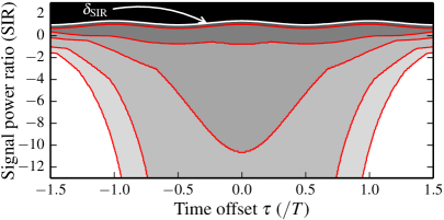
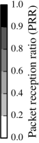
(a) Uncoded transmissions.

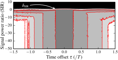
(b) DSSS with hard decision decoding.

(c) DSSS with soft decision decoding.

Figure 8: The capture threshold for colliding packets with identical content depending on the power ratio SIR and the time offset $\tau$. In all three figures, we show the threshold $\delta_{\mathrm{SIR}}$ for identical and uncoded payload as reference. (a) In the uncoded case, the PRR is non-zero in the transitional range, but packet loss is still likely with PRRs of 20–30 %. For coded transmissions, we observe a central area that enables high PRR values (up to 70 % in (b) and approximately 90 % in (c)).

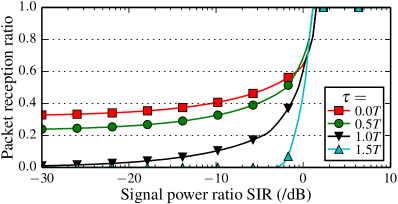
(a) Uncoded transmissions.

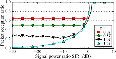
(b) DSSS with hard decision decoding (HDD).

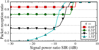
(c) DSSS with soft decision decoding (SDD).

Figure 9: Effect of signal to interference ratio SIR on the PRR for identical payload. Because both use the same payload, only filled markers are present in contrast to 7. (a) For the uncoded case, the PRR varies from approx. 30 % to 100 % and is highly dependent on the SIR. (b) For the HDD case, the PRR takes two values that are more stable across the SIR range: in the negative SIR regime the PRR is around 65 %, and 100 % in the positive SIR regime. (c) For the SDD case, the PRR for negative SIR increases to over 85 % with perfect time synchronization, independent of the SIR.

When considering the collisions of identical packets, we observe very different results (8 and 9): a good reception performance is possible despite even a negative SIR.

Uncoded transmissions. For uncoded transmissions, the PRR performance is shown in 8a. While in this case the threshold for a PRR of 100 % is still equal to the independent payload case, substantially more packets are received in the transitional region with time shifts less than $\pm 0.75T$. However, PRRs around 30 % are usually not sufficient to boost the performance of network protocols. The reason for this limited performance is the carrier phase offset $\varphi_{c}$: with negative SIR, the interfering signal dominates the bit decision at the receiver, and with larger offsets $\varphi_{c}\in\left(\frac{\pi}{2};\frac{3\pi}{2}\right)$, the term $\cos\varphi_{c}$ changes its sign and flips all subsequent bits. In this sense, the literature conjecture that constructive interference is the reason for the good performance of flooding protocols [17, 18] is only valid if the receiver is synchronized to the strongest signal and if the phase offset $\varphi_{c}$ can be neglected. However, because the collisions start during the preamble when using such protocols, successful synchronization cannot be ensured. Therefore, there must be another mechanism that recovers flipped bits.

Hard decision decoding. The reception performance of coded messages provides a hint in this direction (8b). We observe a corridor of $\tau$ values ($\tau=\pm 0.2T$ or 100 ns in IEEE 802.15.4) that has a PRR of 60–80 % in the center (note the larger SIR scale on the y-axis). When two signals with identical payload collide with a small time offset, a reception is still possible even if the interfering signal is far stronger. This suggests that the interfering signal is received instead of the SoI, and that coding helps to overcome bit flips of $\beta_{k}$ induced by the carrier phase. The explanation is a property of Eq. (12): even if all bits are flipped by $\cos\varphi_{c}$, the (absolute) correlation is still maximal for the correct chipping sequence. This shows that DSSS used in IEEE 802.15.4 is a key factor to make the collision-aware protocols work.

Soft decision decoding. The experimentally observed performance in the literature is even superior to 8b [11, 15, 17]. Taking SDD into account, this gap is closed (8c). There is a strong center region for $\tau\leq\pm 0.3T$, or 150 ns in 802.15.4, with a PRR of approximately 90 %. Now, this matches well with existing experimental results. This means that the reception performance is very good in this center region independent of the SIR, i.e., no power control is required and perfect time synchronization is unnecessary for successful reception.

V-B3 Effect of Several Interferers

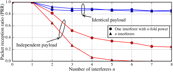
Figure 10: Reception ratio for SDD under one strong interferer or $n$ weaker interferers, but all with equal received power. For identical payload the difference is small, for independent payload several interferers are more destructive than one.

In this subsection, we consider the effect of one strong interferer compared to several interferers with the same power when combined, but evenly distributed across the interferers. We consider the following scenario: all interferers are time-synchronized ($\tau_{i}=0$), but each has an i.i.d. uniform random phase offset $\varphi_{c,i}$ (and independent payload bits $\beta_{k,i}$ if different content is assumed). The interference power varies with $\frac{n}{2}P_{\mathrm{SoI}}$ for a number of interferers $n\in\left\{1,\ldots,8\right\}$, with each interferer having a signal power at the receiver of $\frac{1}{2}P_{\mathrm{SoI}}$.

Under the classical capture threshold model both interference types share the same SIR and thus lead to the same PRR at the receiver. However, as we observe in 10, this is only the case for identical payload, for independent payload $n$ interferers prove to be more destructive despite having the same signal power. While experimental results by Ferrari et al. suggested this result [15, Fig. 12] for identical payload, the root cause is now explained by our model: a single interferer is more likely affected by high attenuation ($\cos\varphi_{c}\approx 0$) than $n$ independent interferers, resulting in a higher likelihood of destructive interference. However, in case of identical payload, even an effective interferer is still received correctly in 90 % of the cases. The observation for independent payload reveals another problem of SINR models: relying on the signal power ratio alone discards the crucial effects of each interferer’s offsets.

V-C Reception of Interfering Signals with Independent Payload

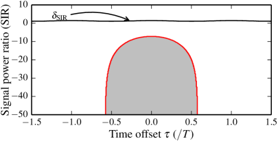
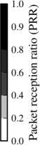
(a) Uncoded transmissions.

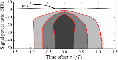
(b) DSSS with hard decision decoding (HDD).

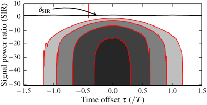
(c) DSSS with soft decision decoding (SDD).

Figure 11: Reception regions of an interfering signal with independent payload. For reference the reception threshold for a synchronized signal $\delta_{\mathrm{SIR}}$ (from 6a) is also shown. (a) In the uncoded case, the packet reception ratio in the central region is 20–30 % because phase and time offsets lead to bit flips in the detected packets. (b) For HDD, the PRR increases to 60–70 % because the coding helps to mitigate bit errors. (c) For SDD, the central region enables a PRR of 80–90 % of the interferer’s packets.

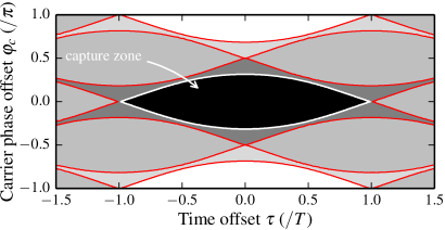
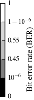
(a) Bit error rate for uncoded transmissions.

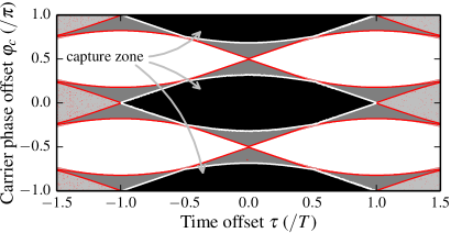
(b) Symbol error rate for DSSS/HDD.

(c) Symbol error rate for DSSS/SDD.

Figure 12: Relation between error rates and signal parameters, time offset $\tau$ and carrier phase offset $\varphi_{c}$ (with $\mathrm{SIR}=-40$ dB). An unsynchronized packet is successfully received if the parameter combinations fall inside the dark capture zones. (a) For uncoded transmissions, the error rate increases for phase offsets $\left|\varphi_{c}\right|>\frac{\pi}{4}$. (b) For coded transmissions and a HDD receiver, the shape of the capture zone is similar to the case in (a), but a second zone around $\varphi_{c}=\pi$ is present. (c) For coded transmission and SDD, the eye shape is widened, and an increasing number of parameter combinations result in error-free transmissions.

Our results explain why and when collision-aware protocols work even without power control: coding enables the reception of interfering signals despite carrier phase and time offsets. In this section, we revisit the case of independent payload but focus our interest now on the reception of the interfering signal, i.e., we treat the interfering signal $u\left(t\right)$ as the SoI and observe the reception of $\beta_{k}$ instead of $\alpha_{k}$. Related work by Pöpper et al. [21] shows that for uncoded systems the reception of interfering signals is indeterministic; in contrast, we show analytically and experimentally (VI) that real systems can receive unsynchronized, interfering packets reliably when using coded messages.

Uncoded transmissions. This case is shown in 11a. In this case, a reception is only successful if bits are not flipped by either $\varphi_{c}$ or $\varphi_{p}$, and we observe a PRR of 20–30 % in the center region ($\mathrm{SIR}<-10$ dB and $\left|\tau\right|<0.5T$) in our evaluation. The reason for the poor reception performance is visible in 12a; the acceptable parameter values of $\tau$ and $\varphi_{c}$ that lead to an error-free packet reception have tight constraints. The interfering signal must hit into a capture zone defined by the signal parameters, which permits the signal to have only small time and carrier phase offsets.

Hard decision decoding. In this setting, the PRR in the central area increases to approx. 60 % (11b). In 12b, we see the reason for the increase: while the general shape is the same, we see a second capture zone around $\varphi_{c}=\pm\pi$. There are two explanations for this. First, we use the same sliced bits from the uncoded case as input for DSSS correlation, which thus possess the same error characteristics. Second, because of the use of absolute correlation values in the correlation (Eq. (12)), the adverse effect of large phase offsets can be repaired. Specifically, this means that even if all bits are flipped, the correlation value is still maximal for the correct chipping sequence. This use of DSSS thus doubles the PRR of an interfering signal.

Soft decision decoding. Finally, in 11c, we see a central area below $\mathrm{SIR}=-23$ dB and a width of $0.25T$ that has a PRR for the interfering signal of approx. 90 %. This means that, if the power difference is large enough, a receiver can ignore a synchronized signal and recover the interfering one despite its offsets. 12c shows this in terms of the capture zone. The eye-shaped regions are much wider compared to the other receiver designs, and especially for the central region with minor deviations of $\tau$, the SER is negligible. Problems in the reception only occur for carrier phase offsets such that $\cos\varphi_{c}\approx 0$. These results show that interfering signals can indeed be received, which helps in collision-aware protocols or other intentional collisions, e.g., in message manipulation attacks on the physical layer. To validate this new result, we present an experimental study of such receptions with real receiver implementations next.

VI Experiments

In this section, we provide experimental evidence that our model accurately captures the behavior of existing receiver implementations. Since many results in the previous section comply with existing experimental results (see also VII), we focus our efforts on the reception of interfering signals because this topic is not well covered experimentally in the literature. We note that we also validated our analytical results with a simulation model based on the numerical integration of time-discrete signals, which confirmed the correctness of our model at the symbol and chip levels. The purpose of this section is to show that our simplifying assumptions, especially for the receiver model, are justified.

VI-A Experimental Setup

To perform this experiment, the requirements for the interferer differ from the scope of operation of Commercial Off-The-Shelf (COTS) devices. We need to (i) transmit arbitrary symbols on the physical layer, without restrictions like PHY headers, (ii) synchronize to ongoing transmissions with high accuracy, and (iii) schedule transmissions at a fine time granularity. To meet these requirements, we implemented a custom software-defined radio based experimental system.

VI-A1 Interferer implementation

To this end, we modified our USRP2-based experimental system RFReact [39] to recover the timing of the other signal and send arbitrary IEEE 802.15.4 symbols at controlled time offsets. Because of its implementation in the USRP2’s FPGA, the system is able to tune the start of transmission with a granularity of 10 ns and send arbitrary waveforms. A detailed description of the system can be found in a technical report [40].

VI-A2 Experimental methodology

In our experiments, we consider three parties in the network: a standard-compliant receiver (we monitor the behavior of two implementations to test for hardware dependencies, Atmel AT86RF230 and TI CC2420), a synchronized sender $\mathcal{S}$ (a COTS RZ Raven USB), and the interferer $\mathcal{I}$ described above. The procedure is as follows: $\mathcal{S}$ sends a packet with PHY headers, MAC header, and 8 byte payload. $\mathcal{I}$ time-synchronizes with this signal and schedules the transmission of 8 different bytes at the beginning of the payload of $\mathcal{S}$. The receiver first synchronizes on $\mathcal{S}$ and receives its header, but experiences a collision in the payload bits. We note that the receivers do not attempt to correct bit errors, retransmissions are used for error recovery during normal operation. Damaged packets are simply detected using the checksum at the end and discarded in case of failure. For the experiments we reconfigured the devices so that all packets are recorded, even if the checksums did not match.

We chose values of $\tau$ in $\left(-1.5T;1.5T\right)$ or $\pm 750$ ns in steps of $10$ ns; for each time offset $\tau$, we sent 1,000 packets and analyzed the payload detected by the receiver. We derived the value of $\tau$ empirically, i.e., we chose the point with maximum PRR in the center as $\tau=0$. We adjusted the transmit power of $\mathcal{I}$ to result in a SIR of $-40$ dB to be in the region of interest.

VI-B Experimental Results

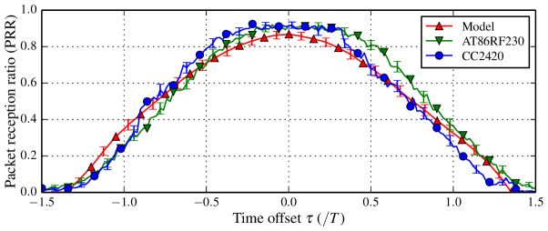
(a) Comparison of packet reception ratios.

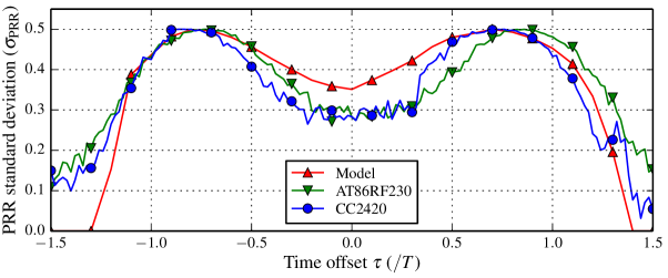
(b) Comparison of PRR standard deviations.

Figure 13: Experimental results for two receivers in terms of packet reception (PRR) performance and PRR standard deviation compared to our model. Both receivers display a behavior that is well-described by the model.

We analyze our measurements using two metrics, packet reception ratio and symbol error rate.

VI-B1 Packet reception ratio (PRR)

Based on the received packet data from the experiments, we derive the PRR as the number of packets with correct payload (of the interferer) divided by the total number of packets. In other words, we measure the empirical success probability for a message manipulation attack. The experimental results for the mean PRR of the two receivers are shown in 13a. We observe a good fit with the predictions of our model to both receivers, Atmel AT86RF230 and TI CC2420. In the central region, the receivers show a slightly better ability to receive the interfering signal than predicted by our analytical model. The reason is that our model makes the assumption that no frequency offset is present and that the receiver does not try to resynchronize with a stronger signal. However, receivers must be able to tolerate frequency offsets of up to 100 kHz [33, $\S$6.9.4] and thus track and possibly correct the phase during the packet reception process. Yet, as the results show, our assumptions still yield a good approximation of the real receiver behavior.

To further validate our model, we perform an analysis of the standard deviation of the measured PRR values (13b). In general, the second order statistics follow the non-trivial shape well. On closer inspection, we observe three regions in the graph. For $\left|\tau\right|<0.5$, our model slightly overestimates the standard deviation; the reason is that the PRR performance of the COTS receivers is better than our model, leading to less variance. For $0.5<\left|\tau\right|<1.1$, the curves are close to each other. Finally, in the zone with $\left|\tau\right|>1.1$, the model slightly underestimates the standard deviation, again because the real receivers perform better than the model predicts. Still, the model provides a good approximation of the behavior of widely used receivers for interfering signals under the assumption of random carrier phase offsets.

VI-B2 Symbol error rate (SER)

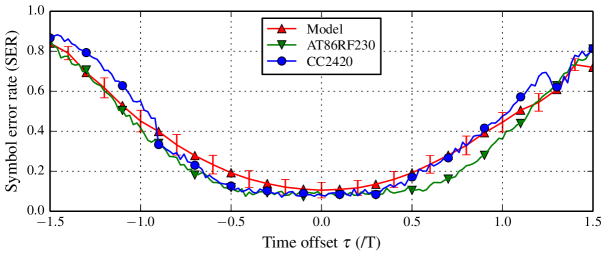
(a) Comparison of symbol error rates.

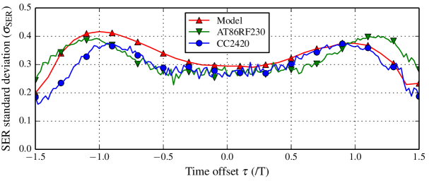
(b) Comparison of SER standard deviations.

Figure 14: Comparison of experimentally measured symbol error rates and standard deviations, and the SER values predicted by our model.

We derive the SER by summation of the number of symbol errors across the payload of all received packets for a given time offset $\tau$, and divide this sum by the total number of payload symbols. This metric gives better insights into the causes for packet errors, and provides another validation for the capture zone. In 14a, we observe that the fit is good for the symbol error rate as well, with a slightly better SER performance for the COTS receivers as expected. Considering the SER standard deviation (14b), we observe a similar behavior as in the PRR case, the predictions of the model and the measured results provide a good fit in both, curve shape and absolute values.

VII Guidelines for Optimal Parameter Settings

Here, we provide a summary of our main findings and highlight key conclusions for the design of protocols that leverage concurrent transmissions. In particular, we summarize how the notion of capture zones enables engineers and protocol designers to choose optimal parameter ranges for signal power ratio, time offset, and carrier phase offset to ensure a successful reception despite collisions.

VII-A Signal to Interference Ratio SIR

Our model confirms that when the SoI is above the SIR threshold $\delta_{\mathrm{SIR}}\approx 2$ dB, then a successful reception is guaranteed (the capture effect). This is consistent with existing results; for the CC2420 transceiver, Gezer et al. [6], Maheshwari et al. [7], Dutta et al. [11], and Son et al. [8] report an experimentally observed threshold of about 3 dB. Considering that their channels were not noise-free and that SINR measurements were collected by the radio transceivers themselves, rather than calibrated measurement equipment such that inaccuracies may arise, this is consistent with our results. If it can be ensured that the stronger signal arrives first and the synchronization process succeeds, the SIR-based capture threshold is a valid model for receiver behavior.

A different matter is the case when the SoI is located in the negative SIR regime, i.e., the interfering signal is stronger than the SoI. This situation occurs if an interferer is closer to the receiver or the synchronization process fails because of a collision during the preamble (which is the case, for example, for the collision-aware flooding protocols). Our model gives better insights in this situation and shows that a reception may still be possible no matter what SIR, given that the interfering signal parameters are in the capture zone as defined by the time offset $\tau$ and carrier phase offset $\varphi_{c}$. Valid settings for these parameters are discussed below.

VII-B Time Offset $\tau$

As a guideline derived from the capture zone, the time offset $\tau$ should be below $T/2$ for successful concurrent transmissions with identical content, which translates to $250$ ns for IEEE 802.15.4. Thus network flooding protocols, for example Glossy, should aim to keep the transmission start time error below this value to ensure a desired PRR above 75 %. If $\tau<200$ ns can be ensured, the achievable PRR is approximately 90 %. We note that this ensures worst-case performance (i.e., the SoI is always in the negative SIR regime). The actual performance may be higher in situations with positive SIR or successful synchronization.

VII-C Carrier Phase Offset $\varphi_{c}$

If the carrier frequency offset at the receiver can be precisely controlled by the senders, there are several options. Interferers can choose $\varphi_{c}\approx\pm\frac{\pi}{2}$ to minimize their effect on the SoI, reducing their influence to signal demodulation. On the other hand, interferers could aim for the capture zone (e.g., $\left|\varphi_{c}\right|<0.4\pi$ or $\left|\varphi_{c}\right|>0.6\pi$ for $\tau=0$ and SDD) to ensure that their signal is received without errors. There are, however, few approaches in the literature that aim to exploit this. The reason is that the carrier phase at another physical location is hard to predict except in static and free space scenarios because of fading and multipath effects. Pöpper et al. [21] show for uncoded QPSK that carrier phase offsets are the major hindrance for a (malicious) interferer to control the bit decisions. In contrast, the results based on our model suggest that such precise phase control is not necessary when DSSS is used, and that intentional message manipulations by deliberate interference are indeed a real threat [41].

VII-D Number of Concurrent Interferers

Our results in V-B3 explain why the number of interferers only has a small impact on reception performance for concurrent transmissions using identical payload. Ferrari et al. [15] observed this behavior in their experiments, achieving a stable PRR above 98 % for 2–10 concurrent transmissions. Maheshwari et al. [7] observed that the SIR threshold is not varying with an increasing number of interferers. On the other hand, Lu and Whitehouse [16] reported a decreasing PRR when the number of interferers is increased. However, the Flash Flooding protocol relies on capture, such that increased time offsets may also influence the results. Some related work claims that a greater number of concurrent transmitters cause problems (Wang et al. [17], Doddavenkatappa et al. [14]) because “the probability of the maximum time displacement across different transmitters exceeding the required threshold for constructive interference” may increase. Our model shows that these protocol-related issues should be addressed with more precise timing synchronization across the network. For independent payload, we show that 2–3 interferers are sufficient to reduce the PRR significantly. This confirms the effect reported by Gezer et al. [6] that the PRR decreases with an increasing number of interferers.

VIII Conclusion

In this article, we presented the first comprehensive analytical model for concurrent transmissions over a wireless channel. As shown in an extensive parameter space exploration, the model recovers insights from experimental results found in the literature and going beyond that, explains the root causes for successful concurrent transmissions exploited in a new generation of sensor network protocols that intentionally generate collisions to increase network throughput or to reduce latency. Our results reveal that power capture alone is not sufficient to explain the performance of such protocols. Rather, coding is an essential factor in the success of these protocols because it crucially widens the capture zone of acceptable signal offsets, increasing the probability of successful reception. Finally, our experimental study of packet reception under collisions shows a good fit and reinforces the validity of our model; as a further contribution, we demonstrated the feasibility of message manipulation attacks over the air experimentally.

Appendix A Integrating Rectangle Pulses

Figure 15: Examples of active bits in the integration interval for the $I$-bit $k$. For $\tau=0$, the only active bit in the integration interval is $\beta_{0}^{I}$. When the signal starts half a bit-length too early ($\tau=-T$), there are two bits $\beta_{0}^{I}$ and $\beta_{1}^{I}$ that contribute equally to the bit decision, both are active for a duration of $T$. In the general case of a time offset $\tau$, there are two active bits with indices $\beta_{k^{\prime}-1}^{I}$ and $\beta_{k^{\prime}}^{I}$, with an active time duration of $\underline{\tau}$ and $2T-\underline{\tau}$, respectively.

A central equation for deriving the influence of individual bits on the demodulator output is the integration of the superposition of time shifted unit pulses $\Pi\left(t\right)$ (defined in (LABEL:Pulse)). This is especially important because of signal time offsets $\tau$ that shift the pulses relative to the integration interval. Situations that arise are shown in 15.

To this end, we first derive the general result to the integration over one bit interval $k$ for arbitrary, integrable functions $f\left(t\right)$. We consider two variants, the integration of in-phase bits, and the special case of integrating quadrature-phase bits in the bounds of $I$-bits (which happens when $Q$-bits leak into the $I$-phase), i.e.,

$$S_{k}^{I}\left(f\right) =\int_{\left(2k-1\right)T}^{\left(2k+1\right)T}b_{I}\left(t-\tau\right)f\left(t\right)dt$$

$$S_{k}^{Q}\left(f\right) =\int_{\left(2k-1\right)T}^{\left(2k+1\right)T}b_{Q}\left(t-\tau\right)f\left(t\right)dt.$$

Our approach is to split each equation into two parts where the unit pulse is the constant 1 function to simplify the equations. Since only one pulse is active at any point in time, such splitting is possible.

A-A Integrating Bit Pulses During the $I$ Integration Interval

A-A1 Integration of $I$-bits

To perform the integration, we first derive the two indices that have active pulses during the integration interval. The shift introduced by $\tau$ lead to the two new bits with indices $k^{\prime}=k-\left\lfloor\frac{\tau}{2T}\right\rfloor$ and $k^{\prime}-1$. The remaining time offset inside the selected bits is $\underline{\tau}=\tau-2k_{\tau}T$, i.e., each of the two bits is active for the time interval $\underline{\tau}$ and $2T-\underline{\tau}$, respectively. Because of this definition, the values of $\underline{\tau}$ are restricted to the interval $\left(0,2T\right)$—negative values would activate previous bits, which is prevented by the floor operation.

For the in-phase component, we derive

$$S_{k}^{I}\left(f\right)$$

$$=\int_{\left(2k-1\right)T}^{\left(2k+1\right)T}b_{I}\left(t-\tau\right)f\left(t\right)dt$$

$$=\int_{\left(2k-1\right)T}^{\left(2k+1\right)T}b_{I}\left(t-2k_{\tau}T-\underline{\tau}\right)f\left(t\right)dt$$

$$=\int_{\left(2k-1\right)T}^{\left(2k+1\right)T}\sum_{k=-\infty}^{\infty}\beta_{k}^{I}\Pi\left(\frac{t-\underline{\tau}-\left(k+k_{\tau}\right)2T}{2T}\right)f\left(t\right)dt$$

$$=\int_{\left(2k-1\right)T}^{\left(2k+1\right)T}\left(\beta_{k-1}^{I}\Pi\left(\frac{t-\underline{\tau}-\left(k-1\right)2T}{2T}\right)+\beta_{k}^{I}\Pi\left(\frac{t-\underline{\tau}-2kT}{2T}\right)\right)f\left(t\right)dt$$

$$=\beta_{k-1}^{I}\int_{\left(2k-1\right)T}^{\left(2k+1\right)T}\Pi\left(\frac{t-\underline{\tau}-\left(k-1\right)2T}{2T}\right)f\left(t\right)dt+\beta_{k}^{I}\int_{\left(2k-1\right)T}^{\left(2k+1\right)T}\Pi\left(\frac{t-\underline{\tau}-2kT}{2T}\right)f\left(t\right)dt$$

$$=\beta_{k-1}^{I}\int_{\left(2k-1\right)T}^{\left(2k-1\right)T+\underline{\tau}}\Pi\left(\frac{t-\underline{\tau}-\left(k-1\right)2T}{2T}\right)f\left(t\right)dt+\beta_{k}^{I}\int_{\left(2k-1\right)T+\underline{\tau}}^{\left(2k+1\right)T}\Pi\left(\frac{t-\underline{\tau}-2kT}{2T}\right)f\left(t\right)dt$$

$$=\beta_{k-1}^{I}\int_{\left(2k-1\right)T}^{\left(2k-1\right)T+\underline{\tau}}f\left(t\right)dt+\beta_{k}^{I}\int_{\left(2k-1\right)T+\underline{\tau}}^{\left(2k+1\right)T}f\left(t\right)dt$$

$$=\beta_{k-1}^{I}\left[F\left(t\right)\vphantom{\prod}\right]_{2kT-T}^{2kT-T+\underline{\tau}}+\beta_{k}^{I}\left[F\left(t\right)\vphantom{\prod}\right]_{2kT-T+\underline{\tau}}^{2kT+T}$$

If the function to integrate is the constant 1 function ($f\left(t\right)=1$), then we derive

$$S_{k}^{I}\left(1\right) =\underline{\tau}\beta_{k-1}^{I}+\left(2T-\underline{\tau}\right)\beta_{k}^{I}$$ (13)

A-A2 Integration of $Q$-bits

When $Q$ bits leak into the in-phase, we have the consider the additional shift of $T$ due to the staggering of bits in the MSK modulation. We provide the derivation of this special case here. First, we substitute the timing offset $\tau$ with $\tau^{Q}=\tau+T$ to accommodate of the staggering. Second, the bit indices must be re-adjusted because of the shift; the new index is denoted by $k^{Q\prime}=k-\left\lfloor\left(\tau+T\right)/2T\right\rfloor$. For the case of the constant 1 function, we derive then

$$S_{k}^{Q}\left(1\right) =\underline{\tau^{Q}}\beta_{k^{Q\prime}-1}^{Q}+\left(2T-\underline{\tau^{Q}}\right)\beta_{k^{Q\prime}}^{Q}.$$ (14)

A-B Deriving Special Cases: $S_{k}^{I}\left(\cos 2\omega_{p}t\right)$ and $S_{k}^{Q}\left(\cos 2\omega_{p}t\right)$

A-B1 Integration of $I$-bits

We derive the result of bit pulse integration for this special case.

$$S_{k}^{I}\left(\cos 2\omega_{p}t\right)$$

$$=\int_{\left(2k-1\right)T}^{\left(2k+1\right)T}b_{I}\left(t-\tau\right)\cos 2\omega_{p}t\>dt$$

$$=\beta_{k-1}^{I}\left[\frac{1}{2\omega_{p}}\sin 2\omega_{p}t\vphantom{\prod}\right]_{\left(2k-1\right)T}^{\left(2k-1\right)T+\underline{\tau}}+\beta_{k}^{I}\left[\frac{1}{2\omega_{p}}\sin 2\omega_{p}t\vphantom{\prod}\right]_{\left(2k-1\right)T+\underline{\tau}}^{\left(2k+1\right)T}$$

$$=\frac{\beta_{k-1}^{I}}{2\omega_{p}}\left[\sin 2\omega_{p}t\vphantom{\prod}\right]_{\left(2k-1\right)T}^{\left(2k-1\right)T+\underline{\tau}}+\frac{\beta_{k}^{I}}{2\omega_{p}}\left[\sin 2\omega_{p}t\vphantom{\prod}\right]_{\left(2k-1\right)T+\underline{\tau}}^{\left(2k+1\right)T}$$

Performing the integration results in (we denote $\omega_{p}\underline{\tau}=\underline{\varphi_{p}}$):

$$=\frac{\beta_{k-1}^{I}}{2\omega_{p}}\left[\sin\left(\left(2k-1\right)\pi+2\underline{\varphi_{p}}\right)-\sin\left(\left(2k-1\right)\pi\right)\right]$$

$$\hphantom{=}+\frac{\beta_{k}^{I}}{2\omega_{p}}\left[\sin\left(\left(2k+1\right)\pi\right)-\sin\left(\left(2k-1\right)\pi+2\underline{\varphi_{p}}\right)\right]$$

$$=\frac{\beta_{k-1}^{I}}{2\omega_{p}}\left[\sin\left(-\pi+2\underline{\varphi_{p}}\right)-\sin\left(-\pi\right)\right]+\frac{\beta_{k}^{I}}{2\omega_{p}}\left(\sin\pi+\sin 2\underline{\varphi_{p}}\right)$$

$$=-\frac{\beta_{k-1}^{I}}{2\omega_{p}}\sin 2\underline{\varphi_{p}}+\frac{\beta_{k}^{I}}{2\omega_{p}}\sin 2\underline{\varphi_{p}}$$

$$=\sin 2\underline{\varphi_{p}}\left(-\frac{\beta_{k-1}^{I}}{2\omega_{p}}+\frac{\beta_{k}^{I}}{2\omega_{p}}\right)$$

$$=-\frac{1}{2\omega_{p}}\sin 2\varphi_{p}\left(\beta_{k-1}^{I}-\beta_{k}^{I}\right)$$

The overall result is

$$S_{k}^{I}\left(\cos 2\omega_{p}t\right) =-\frac{1}{2\omega_{p}}\sin 2\varphi_{p}\left(\beta_{k-1}^{I}-\beta_{k}^{I}\right)$$ (15)

A-B2 Integration of $Q$-bits

In this case, the use of $\tau^{Q}$ leads to a different phase shift $\varphi_{p}^{Q}=\omega_{p}\left(\tau+T\right)=\omega_{p}\tau+\frac{\pi T}{2T}=\varphi_{p}+\frac{\pi}{2}$ that leads to changes in the integration. Using the following two simplifications the derivation can be performed analogously to the previous subsection.

$$\sin 2\underline{\varphi_{p}^{Q}} =\sin 2\omega_{p}\underline{\tau^{Q}}=\sin\left(2\frac{\pi}{2T}\left(\tau^{Q}-2k_{\tau}^{Q}T\right)\right)=\sin\left(\frac{\tau^{Q}\pi}{T}-2k_{\tau}^{Q}\pi\right)=\sin 2\varphi_{p}^{Q}$$

$$\sin 2\varphi_{p}^{Q} =\sin\left(2\varphi_{p}+\pi\right)=-\sin 2\varphi_{p}$$

The overall result is

$$S_{k}^{Q}\left(\cos 2\omega_{p}t\right) =\frac{1}{2\omega_{p}}\sin 2\varphi_{p}\left(\beta_{k^{Q\prime}-1}^{Q}-\beta_{k^{Q\prime}}^{Q}\right)$$ (16)

A-C Deriving Special Cases: $S_{k}^{I}\left(\sin 2\omega_{p}t\right)$ and $S_{k}^{Q}\left(\sin 2\omega_{p}t\right)$

A-C1 Integration of $I$-bits

We derive the result of bit pulse integration for this special case.

$$S_{k}^{I}\left(\sin 2\omega_{p}t\right)$$

$$=\int_{\left(2k-1\right)T}^{\left(2k+1\right)T}b_{I}\left(t-\tau\right)\sin 2\omega_{p}t\>dt$$

$$=\beta_{k-1}^{I}\left[-\frac{1}{2\omega_{p}}\cos 2\omega_{p}t\vphantom{\prod}\right]_{\left(2k-1\right)T}^{\left(2k-1\right)T+\underline{\tau}}+\beta_{k}^{I}\left[-\frac{1}{2\omega_{p}}\cos 2\omega_{p}t\vphantom{\prod}\right]_{\left(2k-1\right)T+\underline{\tau}}^{\left(2k+1\right)T}$$

$$=-\frac{\beta_{k-1}^{I}}{2\omega_{p}}\left[\cos 2\omega_{p}t\vphantom{\prod}\right]_{\left(2k-1\right)T}^{\left(2k-1\right)T+\underline{\tau}}-\frac{\beta_{k}^{I}}{2\omega_{p}}\left[\cos 2\omega_{p}t\vphantom{\prod}\right]_{\left(2k-1\right)T+\underline{\tau}}^{\left(2k+1\right)T}$$

Performing the integration results in (we denote $\omega_{p}\underline{\tau}=\underline{\varphi_{p}}$):

$$=-\frac{\beta_{k-1}^{I}}{2\omega_{p}}\left[\cos\left(\left(2k-1\right)\pi+2\underline{\varphi_{p}}\right)-\cos\left(\left(2k-1\right)\pi\right)\right]$$

$$\hphantom{=}-\frac{\beta_{k}^{I}}{2\omega_{p}}\left[\cos\left(\left(2k+1\right)\pi\right)-\cos\left(\left(2k-1\right)\pi+2\underline{\varphi_{p}}\right)\right]$$

$$=-\frac{\beta_{k-1}^{I}}{2\omega_{p}}\left(\cos\left(-\pi+2\underline{\varphi_{p}}\right)-\cos\left(-\pi\right)\right)-\frac{\beta_{k}^{I}}{2\omega_{p}}\left(\cos\pi-\cos\left(-\pi+2\underline{\varphi_{p}}\right)\right)$$

$$=-\frac{\beta_{k-1}^{I}}{2\omega_{p}}\left(1-\cos 2\underline{\varphi_{p}}\right)+\frac{\beta_{k}^{I}}{2\omega_{p}}\left(1-\cos 2\underline{\varphi_{p}}\right)$$

$$=-\frac{1}{2\omega_{p}}\left(1-\cos 2\underline{\varphi_{p}}\right)\left(\beta_{k-1}^{I}-\beta_{k}^{I}\right)$$

$$=-\frac{1}{2\omega_{p}}\left(1-\cos 2\varphi_{p}\right)\left(\beta_{k-1}^{I}-\beta_{k}^{I}\right)$$

The overall result is

$$S_{k}^{I}\left(\sin 2\omega_{p}t\right) =-\frac{1}{2\omega_{p}}\left(1-\cos 2\varphi_{p}\right)\left(\beta_{k-1}^{I}-\beta_{k}^{I}\right)$$ (17)

A-C2 Integration of $Q$-bits

This case can be performed analogously to A-B, with the following two simplifications:

$$\cos 2\underline{\varphi_{p}^{Q}} =\cos 2\omega_{p}\underline{\tau^{Q}}=\cos\left(2\frac{\pi}{2T}\left(\tau^{Q}-2k_{\tau}^{Q}T\right)\right)=\cos\left(\frac{\tau^{Q}\pi}{T}-2k_{\tau}^{Q}\pi\right)=\cos 2\varphi_{p}^{Q}$$

$$\cos 2\varphi_{p}^{Q} =\cos\left(2\varphi_{p}+\pi\right)=-\cos 2\varphi_{p}$$

The overall result is

$$S_{k}^{Q}\left(\sin 2\omega_{p}\left(t\right)\right) =-\frac{1}{2\omega_{p}}\left(1+\cos 2\varphi_{p}\right)\left(\beta_{k^{Q\prime}-1}^{Q}-\beta_{k^{Q\prime}}^{Q}\right)$$ (18)

Appendix B Demodulator Output for Signals with Both Offsets $\tau,\varphi_{c}$

With the tools presented in A, we can now proceed to prove 1.

Theorem 1.

For an interfering MSK signal $u\left(t\right)$ with parameters $\tau$ and $\varphi_{c}$, the contribution to the demodulation output $\Lambda_{u}^{I}\left(k\right)$ is given by

$$\Lambda_{u}^{I}\left(k\right) =\frac{1}{4}A_{u}\left\{\cos\varphi_{c}\left[\cos\varphi_{p}\left(\underline{\tau}\beta_{k-1}^{I}+\left(2T-\underline{\tau}\right)\beta_{k}^{I}\right)-\frac{2T}{\pi}\sin\varphi_{p}\left(\beta_{k-1}^{I}-\beta_{k}^{I}\right)\right]\right.$$

$$\hphantom{=\frac{1}{4}A_{u}}\left.-\sin\varphi_{c}\left[\sin\varphi_{p}\left(\underline{\tau^{Q}}\beta_{k^{Q\prime}-1}^{Q}+\left(2T-\underline{\tau^{Q}}\right)\beta_{k^{Q\prime}}^{Q}\right)+\frac{2T}{\pi}\cos\varphi_{p}\left(\beta_{k^{Q\prime}-1}^{Q}-\beta_{k^{Q\prime}}^{Q}\right)\right]\right\}.$$

Proof:

We first derive the resulting signal after demodulation ((LABEL:Lambda)).

$$u\left(t\right)\phi_{I}\left(t\right)$$

$$=A_{u}\left[b_{I}\left(t-\tau\right)\cos\left(\omega_{p}t-\varphi_{p}\right)\cos\left(\omega_{c}t+\varphi_{c}\right)\right.$$

$$\hphantom{=A_{u}}\left.+b_{Q}\left(t-\tau\right)\sin\left(\omega_{p}t-\varphi_{p}\right)\sin\left(\omega_{c}t+\varphi_{c}\right)\right]\left[\cos\omega_{p}t\cos\omega_{c}t\right]$$

$$=A_{u}\left[\left(b_{I}\left(t-\tau\right)\cos\left(\omega_{p}t-\varphi_{p}\right)\cos\omega_{p}t\cos\left(\omega_{c}t+\varphi_{c}\right)\cos\omega_{c}t\right)\right.$$

$$\hphantom{=A_{u}}\left.+\left(b_{Q}\left(t-\tau\right)\sin\left(\omega_{p}t-\varphi_{p}\right)\cos\omega_{p}t\sin\left(\omega_{c}t+\varphi_{c}\right)\cos\omega_{c}t\right)\right]$$

$$=\frac{A_{u}}{4}\left[\left(b_{I}\left(t-\tau\right)\left(\cos\varphi_{p}+\cos\left(2\omega_{p}t-\varphi_{p}\right)\right)\left(\cos\varphi_{c}+\cos\left(2\omega_{c}t+\varphi_{c}\right)\right)\right)\right.$$

$$\hphantom{=\frac{A_{u}}{4}}\left.+\left(b_{Q}\left(t-\tau\right)\left(\sin\left(-\varphi_{p}\right)+\sin\left(2\omega_{p}t-\varphi_{p}\right)\right)\left(\sin\varphi_{c}+\sin\left(2\omega_{c}t+\varphi_{c}\right)\right)\right)\right]$$

$$\overset{\star}{=}\frac{A_{u}}{4}\left[\left(b_{I}\left(t-\tau\right)\cos\varphi_{c}\left(\cos\varphi_{p}+\cos\left(2\omega_{p}t-\varphi_{p}\right)\right)\right)\right.$$

$$\hphantom{=\frac{A_{u}}{4}}\left.+\left(b_{Q}\left(t-\tau\right)\sin\varphi_{c}\left(\sin\left(2\omega_{p}t-\varphi_{p}\right)-\sin\varphi_{p}\right)\right)\right]$$

$$=\frac{A_{u}}{4}\left[\left(b_{I}\left(t-\tau\right)\cos\varphi_{c}\left(\cos\varphi_{p}+\cos 2\omega_{p}t\cos\varphi_{p}+\sin 2\varphi_{p}t\sin\varphi_{p}\right)\right)\right.$$

$$\hphantom{=\frac{A_{u}}{4}}\left.+\left(b_{Q}\left(t-\tau\right)\sin\varphi_{c}\left(-\sin\varphi_{p}+\sin 2\omega_{p}t\cos\varphi_{p}-\cos 2\omega_{p}t\sin\varphi_{p}\right)\right)\right]$$

The bit decision is performed by integration over the bit interval $k$.

$$\int_{\left(2k-1\right)T}^{\left(2k+1\right)T}u\left(t\right)\phi_{I}\left(t\right)dt$$

$$=\frac{A_{u}}{4}\left[\cos\varphi_{c}\int_{\left(2k-1\right)T}^{\left(2k+1\right)T}b_{I}\left(t-\tau\right)\left(\cos\varphi_{p}+\cos 2\omega_{p}t\cos\varphi_{p}+\sin 2\varphi_{p}t\sin\varphi_{p}\right)dt\right.$$

$$\hphantom{=\frac{A_{u}}{4}}\left.+\sin\varphi_{c}\int_{\left(2k-1\right)T}^{\left(2k+1\right)T}b_{Q}\left(t-\tau\right)\left(-\sin\varphi_{p}+\sin 2\omega_{p}t\cos\varphi_{p}-\cos 2\omega_{p}t\sin\varphi_{p}\right)dt\right]$$

$$=\frac{A_{u}}{4}\left[\cos\varphi_{c}\mathcal{X}_{1}+\sin\varphi_{c}\mathcal{X}_{2}\right]$$

We derive the results for both terms $\mathcal{X}_{1}$ and $\mathcal{X}_{2}$ individually in the following two sections.

Putting the two results in (LABEL:X1) and (LABEL:X2) together, the overall result is

$$\int_{\left(2k-1\right)T}^{\left(2k+1\right)T}u\left(t\right)\phi_{I}\left(t\right)dt$$

$$=\frac{A_{u}}{4}\left\{\cos\varphi_{c}\left[\cos\varphi_{p}\left(\underline{\tau}\beta_{k-1}^{I}+\left(2T-\underline{\tau}\right)\beta_{k}^{I}\right)-\frac{2T}{\pi}\sin\varphi_{p}\left(\beta_{k-1}^{I}-\beta_{k}^{I}\right)\right]\right.$$

$$\hphantom{=\frac{A_{u}}{4}}\left.-\sin\varphi_{c}\left[\sin\varphi_{p}\left(\underline{\tau^{Q}}\beta_{k^{Q\prime}-1}^{Q}+\left(2T-\underline{\tau^{Q}}\right)\beta_{k^{Q\prime}}^{Q}\right)+\frac{2T}{\pi}\cos\varphi_{p}\left(\beta_{k^{Q\prime}-1}^{Q}-\beta_{k^{Q\prime}}^{Q}\right)\right]\right\}$$

∎

B-A Integrating the Term $\mathcal{X}_{1}$

$$\int_{\left(2k-1\right)T}^{\left(2k+1\right)T}b_{I}\left(t-\tau\right)\left(\cos\varphi_{p}+\cos 2\omega_{p}t\cos\varphi_{p}+\sin 2\varphi_{p}t\sin\varphi_{p}\right)dt$$

$$=\cos\varphi_{p}\int_{\left(2k-1\right)T}^{\left(2k+1\right)T}b_{I}\left(t-\tau\right)dt+\cos\varphi_{p}\int_{\left(2k-1\right)T}^{\left(2k+1\right)T}b_{I}\left(t-\tau\right)\cos 2\omega_{p}t\>dt$$

$$\hphantom{=}+\sin\varphi_{p}\int_{\left(2k-1\right)T}^{\left(2k+1\right)T}b_{I}\left(t-\tau\right)\sin 2\omega_{p}t\>dt$$

$$=\cos\varphi_{p}S_{k}^{I}\left(1\right)+\cos\varphi_{p}S_{k}^{I}\left(\cos 2\omega_{p}t\right)+\sin\varphi_{p}S_{k}^{I}\left(\sin 2\omega_{p}t\right)$$

By using the results in A ((LABEL:Rect1-I,RectCos-I,RectSin-I)), we can reformulate this equation to

$$=\cos\varphi_{p}\left(\underline{\tau}\beta_{k-1}^{I}+\left(2T-\underline{\tau}\right)\beta_{k}^{I}\right)$$

$$\hphantom{=}-\frac{\beta_{k-1}^{I}}{2\omega_{p}}\left(\cos\varphi_{p}\sin 2\varphi_{p}+\sin\varphi_{p}\left(1-\cos 2\varphi_{p}\right)\right)+\frac{\beta_{k}^{I}}{2\omega_{p}}\left(\cos\varphi_{p}\sin 2\varphi_{p}+\sin\varphi_{p}\left(1-\cos 2\varphi_{p}\right)\right)$$

Simplifying this equation yields the desired result.

$$=\cos\varphi_{p}\left(\underline{\tau}\beta_{k-1}^{I}+\left(2T-\underline{\tau}\right)\beta_{k}^{I}\right)-\left(\frac{\beta_{k-1}^{I}-\beta_{k}^{I}}{2\omega_{p}}\right)\left(\sin 2\varphi_{p}\cos\varphi_{p}-\cos 2\varphi_{p}\sin\varphi_{p}+\sin\varphi_{p}\right)$$

$$=\cos\varphi_{p}\left(\underline{\tau}\beta_{k-1}^{I}+\left(2T-\underline{\tau}\right)\beta_{k}^{I}\right)-\frac{\sin\varphi_{p}}{\omega_{p}}\left(\beta_{k-1}^{I}-\beta_{k}^{I}\right)$$

$$=\cos\varphi_{p}\left(\underline{\tau}\beta_{k-1}^{I}+\left(2T-\underline{\tau}\right)\beta_{k}^{I}\right)-\frac{2T}{\pi}\sin\varphi_{p}\left(\beta_{k-1}^{I}-\beta_{k}^{I}\right)$$

In the second step in the previous derivation, we used the following simplification:

$$\sin 2\varphi_{p}\cos\varphi_{p}-\cos 2\varphi_{p}\sin\varphi_{p}+\sin\varphi_{p}$$

$$=2\cos^{2}\varphi_{p}\sin\varphi_{p}-\left(2\cos^{2}\varphi_{p}-1\right)\sin\varphi_{p}+\sin\varphi_{p}$$

$$=\left(2\cos^{2}\varphi_{p}-2\cos^{2}\varphi_{p}+1+1\right)\sin\varphi_{p}$$

$$=2\sin\varphi_{p}$$

Overall, the result is

$$\mathcal{X}_{1} =\cos\varphi_{p}\left(\underline{\tau}\beta_{k-1}^{I}+\left(2T-\underline{\tau}\right)\beta_{k}^{I}\right)-\frac{2T}{\pi}\sin\varphi_{p}\left(\beta_{k-1}^{I}-\beta_{k}^{I}\right)$$ (19)

B-B Integrating the Term $\mathcal{X}_{2}$

We will now derive the second integral. We must use the rules for $Q$ pulse integration with $I$ intervals (A-A2).

$$\int_{\left(2k-1\right)T}^{\left(2k+1\right)T}b_{Q}\left(t-\tau\right)\left(-\sin\varphi_{p}-\cos 2\omega_{p}t\sin\varphi_{p}+\sin 2\omega_{p}t\cos\varphi_{p}\right)dt$$

$$=-\left[\int_{\left(2k-1\right)T}^{\left(2k+1\right)T}b_{Q}\left(t-\tau\right)\sin\varphi_{p}dt+\int_{\left(2k-1\right)T}^{\left(2k+1\right)T}b_{Q}\left(t-\tau\right)\cos 2\omega_{p}t\sin\varphi_{p}dt\right.$$

$$\hphantom{=-}\left.-\int_{\left(2k-1\right)T}^{\left(2k+1\right)T}b_{Q}\left(t-\tau\right)\sin 2\omega_{p}t\cos\varphi_{p}dt\right]$$

$$=-\left[\sin\varphi_{p}S_{k}^{Q}\left(1\right)+\sin\varphi_{p}S_{k}^{Q}\left(\cos 2\omega_{p}t\right)-\cos\varphi_{p}S_{k}^{Q}\left(\sin 2\omega_{p}t\right)\right]$$

By using the results in A ((LABEL:Rect1-Q,RectCos-Q,RectSin-Q)), we can reformulate this equation to

$$=-\sin\varphi_{p}\left(\underline{\tau^{Q}}\beta_{k^{Q\prime}-1}^{Q}+\left(2T-\underline{\tau^{Q}}\right)\beta_{k^{Q\prime}}^{Q}\right)$$

$$\hphantom{=}-\frac{1}{2\omega_{p}}\left(\sin\varphi_{p}\sin 2\varphi_{p}+\cos\varphi_{p}\left(1+\cos 2\varphi_{p}\right)\right)\left(\beta_{k^{Q\prime}-1}^{Q}-\beta_{k^{Q\prime}}^{Q}\right)$$

$$=-\sin\varphi_{p}\left(\underline{\tau^{Q}}\beta_{k^{Q\prime}-1}^{Q}+\left(2T-\underline{\tau^{Q}}\right)\beta_{k^{Q\prime}}^{Q}\right)$$

$$\hphantom{=}-\frac{1}{2\omega_{p}}\left(\sin 2\varphi_{p}\sin\varphi_{p}+\cos 2\varphi_{p}\cos\varphi_{p}+\cos\varphi_{p}\right)\left(\beta_{k^{Q\prime}-1}^{Q}-\beta_{k^{Q\prime}}^{Q}\right)$$

$$=-\left[\sin\varphi_{p}\left(\underline{\tau^{Q}}\beta_{k^{Q\prime}-1}^{Q}+\left(2T-\underline{\tau^{Q}}\right)\beta_{k^{Q\prime}}^{Q}\right)+\frac{2T}{\pi}\cos\varphi_{p}\left(\beta_{k^{Q\prime}-1}^{Q}-\beta_{k^{Q\prime}}^{Q}\right)\right]$$

In the last step, we used the following simplification

$$\sin 2\varphi_{p}\sin\varphi_{p}+\cos\varphi_{p}+\cos 2\varphi_{p}\cos\varphi_{p}$$

$$=2\sin^{2}\varphi_{p}\cos\varphi_{p}+\cos\varphi_{p}+\left(1-2\sin^{2}\varphi_{p}\right)\cos\varphi_{p}$$

$$=\left(2\sin^{2}\varphi_{p}+1+1-2\sin^{2}\varphi_{p}\right)\cos\varphi_{p}$$

$$=2\cos\varphi_{p}$$

Overall, the result is

$$\mathcal{X}_{2} =-\left[\sin\varphi_{p}\left(\underline{\tau^{Q}}\beta_{k^{Q\prime}-1}^{Q}+\left(2T-\underline{\tau^{Q}}\right)\beta_{k^{Q\prime}}^{Q}\right)+\frac{2T}{\pi}\cos\varphi_{p}\left(\beta_{k^{Q\prime}-1}^{Q}-\beta_{k^{Q\prime}}^{Q}\right)\right]$$ (20)

References

- [1] K. Leentvaar and J. Flint, “The capture effect in FM receivers,” IEEE Trans. Commun., vol. 24, pp. 531–539, May 1976.
- [2] J. Foo and D. Huang, “Multiuser diversity with capture for wireless networks: Protocol and performance analysis,” IEEE J. Sel. Areas Commun., vol. 26, pp. 1386–1396, Oct. 2008.
- [3] R. Gummadi, D. Wetherall, B. Greenstein, and S. Seshan, “Understanding and mitigating the impact of RF interference on 802.11 networks,” in Proc. ACM SIGCOMM ’07, pp. 385–396, Sept. 2007.
- [4] A. Kochut, A. Vasan, A. Shankar, and A. Agrawala, “Sniffing out the correct physical layer capture model in 802.11b,” in Proc. IEEE ICNP ’04, pp. 252–261, Oct. 2004.
- [5] J. Lee, W. Kim, S.-J. Lee, D. Jo, J. Ryu, T. Kwon, and Y. Choi, “An experimental study on the capture effect in 802.11a networks,” in Proc. ACM WinTECH ’07, pp. 19–26, Sept. 2007.
- [6] C. Gezer, C. Buratti, and R. Verdone, “Capture effect in IEEE 802.15.4 networks: Modelling and experimentation,” in Proc. IEEE ISWPC ’10, pp. 204–209, May 2010.
- [7] R. Maheshwari, S. Jain, and S. R. Das, “A measurement study of interference modeling and scheduling in low-power wireless networks,” in Proc. ACM SenSys ’08, pp. 141–154, Nov. 2008.
- [8] D. Son, B. Krishnamachari, and J. Heidemann, “Experimental study of concurrent transmission in wireless sensor networks,” in Proc. ACM SenSys ’06, pp. 237–250, Nov. 2006.
- [9] M. Sha, G. Xing, G. Zhou, S. Liu, and X. Wang, “C-MAC: Model-driven concurrent medium access control for wireless sensor networks,” in Proc. IEEE INFOCOM ’09, pp. 1845–1853, Apr. 2009.
- [10] M. Vutukuru, K. Jamieson, and H. Balakrishnan, “Harnessing exposed terminals in wireless networks,” in Proc. USENIX NSDI ’08, pp. 59–72, Apr. 2008.
- [11] P. Dutta, S. Dawson-Haggerty, Y. Chen, C.-J. M. Liang, and A. Terzis, “Design and evaluation of a versatile and efficient receiver-initiated link layer for low-power wireless,” in Proc. ACM SenSys ’10, pp. 1–14, ACM, Nov. 2010.
- [12] P. Dutta, R. Musaloiu-E., I. Stoica, and A. Terzis, “Wireless ACK collisions not considered harmful,” in Proc. ACM SIGCOMM HotNets-VII, pp. 4:1–6, Oct. 2008.
- [13] D. Wu, C. Dong, S. Tang, H. Dai, and G. Chen, “Fast and fine-grained counting and identification via constructive interference in WSNs,” in Proc. IEEE/ACM IPSN ’14, pp. 191–202, Apr. 2014.
- [14] M. Doddavenkatappa, M. C. Chan, and B. Leong, “Splash: Fast data dissemination with constructive interference in wireless sensor networks,” in Proc. USENIX NSDI ’13, pp. 269–282, Apr. 2013.
- [15] F. Ferrari, M. Zimmerling, L. Thiele, and O. Saukh, “Efficient network flooding and time synchronization with Glossy,” in Proc. IPSN ’11, pp. 73–84, Apr. 2011.
- [16] J. Lu and K. Whitehouse, “Flash Flooding: Exploiting the capture effect for rapid flooding in wireless sensor networks,” in Proc. IEEE INFOCOM ’09, pp. 2491–2499, Apr. 2009.
- [17] Y. Wang, Y. He, X. Mao, Y. Liu, and X. Li, “Exploiting constructive interference for scalable flooding in wireless networks,” IEEE/ACM Trans. Netw., vol. 21, pp. 1880–1889, Dec. 2013.
- [18] Y. Wang, Y. Liu, Y. He, X.-Y. Li, and D. Cheng, “Disco: Improving packet delivery via deliberate synchronized contructive interference,” IEEE Trans. Parallel Distrib. Syst., 2014. To appear.
- [19] N. Santhapuri, S. Nelakuditi, and R. R. Choudhury, “On spatial reuse and capture in ad hoc networks,” in Proc. IEEE WCNC ’08, pp. 1628–1633, Apr. 2008.
- [20] D. Davis and S. Gronemeyer, “Performance of slotted ALOHA random access with delay capture and randomized time of arrival,” IEEE Trans. Commun., vol. 28, pp. 703–710, May 1980.
- [21] C. Pöpper, N. O. Tippenhauer, B. Danev, and S. Čapkun, “Investigation of signal and message manipulations on the wireless channel,” in Computer Security – ESORICS 2011, no. 6879 in LNCS, pp. 40–59, Springer, Sept. 2011.
- [22] K. Whitehouse, A. Woo, F. Jiang, J. Polastre, and D. Culler, “Exploiting the capture effect for collision detection and recovery,” in Proc. IEEE EmNetS-II, pp. 45–52, May 2005.
- [23] D. Yuan and M. Hollick, “Let’s talk together: Understanding concurrent transmissions in wireless sensor networks,” in Proc. IEEE LCN ’13, pp. 219–227, Oct. 2013.
- [24] M. Zimmerling, F. Ferrari, L. Mottola, and L. Thiele, “On modeling low-power wireless protocols based on synchronous packet transmissions,” in Proc. IEEE MASCOTS ’13, pp. 546–555, Aug. 2013.
- [25] K. Jamieson and H. Balakrishnan, “PPR: Partial packet recovery for wireless networks,” in Proc. ACM SIGCOMM ’07, pp. 409–420, Sept. 2007.
- [26] F. Schmidt, M. Ceriotti, and K. Wehrle, “Bit error distribution and mutation patterns of corrupted packets in low-power wireless networks,” in Proc. ACM WiNTECH ’13, pp. 49–56, Sept. 2013.
- [27] K. Wu, H. Tan, H.-L. Ngan, Y. Liu, and L. M. Ni, “Chip error pattern analysis in IEEE 802.15.4,” IEEE Trans. Mob. Comput., vol. 11, pp. 543–552, Apr. 2012.
- [28] P. Gupta and P. R. Kumar, “The capacity of wireless networks,” IEEE Trans. Inf. T., vol. 46, pp. 388–404, May 2000.
- [29] P. Cardieri, “Modeling interference in wireless ad hoc networks,” IEEE Commun. Surveys Tutorials, vol. 12, pp. 551–572, Sept. 2010.
- [30] A. Iyer, C. Rosenberg, and A. Karnik, “What is the right model for wireless channel interference?,” IEEE Trans. Wireless Commun., vol. 8, pp. 2662–2671, June 2009.
- [31] J. Manweiler, N. Santhapuri, S. Sen, R. R. Choudhury, S. Nelakuditi, and K. Munagala, “Order matters: Transmission reordering in wireless networks,” IEEE/ACM Trans. Netw., vol. 20, pp. 353–366, Apr. 2012.
- [32] J. Proakis and M. Salehi, Digital Communications. New York, NY: McGraw-Hill, 5th ed., Nov. 2007.
- [33] “IEEE Standard 802 Part 15.4: Wireless medium access control and physical layer specifications for low-rate WPANs, Sept. 2006..”
- [34] S. Pasupathy, “Minimum shift keying: A spectrally efficient modulation,” IEEE Comm. Mag., vol. 17, pp. 14–22, July 1979.
- [35] T. Schmid, “GNU Radio 802.15.4 en- and decoding,” Tech. Rep. TR-UCLA-NESL-200609-06, UCLA NESL, 2005.
- [36] R. K. Jain, The Art of Computer Systems Performance Analysis: Techniques for Experimental Design, Measurement, Simulation, and Modeling. Hoboken, NJ: John Wiley & Sons, Apr. 1991.
- [37] T. S. Rappaport, Wireless Communications: Principles and Practice. Upper Saddle River, NJ: Prentice-Hall, 2nd ed., Apr. 1996.
- [38] R. A. Poisel, Modern Communications Jamming: Principles and Techniques. Boston, MA: Artech House Publishers, Nov. 2003.
- [39] M. Wilhelm, I. Martinovic, J. B. Schmitt, and V. Lenders, “WiSec ’11 demo: RFReact—a real-time capable and channel-aware jamming platform,” SIGMOBILE Mobile Comp. Commun. Rev., vol. 15, pp. 41–42, Nov. 2011.
- [40] M. Wilhelm, I. Martinovic, J. B. Schmitt, and V. Lenders, “Air dominance in sensor networks: Guarding sensor motes using selective interference,” Tech. Rep. arXiv:1305.4038, TU Kaiserslautern, Germany, May 2013.
- [41] M. Wilhelm, J. B. Schmitt, and V. Lenders, “Practical message manipulation attacks in IEEE 802.15.4 wireless networks,” in Workshop Proc. MMB ’12, pp. 29–31, Mar. 2012.