Unifying neutron stars: getting to GUNS

Abstract

The variety of the observational appearance of young isolated neutron stars must find an explanation in the framework of some unifying approach. Nowadays it is believed that such scenario must include magnetic field decay, the possibility of magnetic field emergence on a time scale $\lesssim 10^{4}$–$10^{5}$ yrs, significant contribution of non-dipolar fields, and appropriate initial parameter distributions. We present our results on the initial spin period distribution, and suggest that inconsistences between distributions derived by different methods for samples with different average ages can uncover field decay or/and emerging field. We describe a new method to probe the magnetic field decay in normal pulsars. The method is a modified pulsar current approach, where we study pulsar flow along the line of increasing characteristic age for constant field. Our calculations, performed with this method, can be fitted with an exponential decay for ages in the range $8\times 10^{4}$–$3.5\times 10^{5}$ yrs with a time scale $\sim 5\times 10^{5}$ yrs. We discuss several issues related to the unifying scenario. At first, we note that the dichotomy, among local thermally emitting neutron stars, between normal pulsars and the Magnificent Seven remains unexplained. Then we discuss the role of high-mass X-ray binaries in the unification of neutron star evolution. We note, that such systems allow to check evolutionary effects on a time scale longer than what can be probed with normal pulsars alone. We conclude with a brief discussion of importance of discovering old neutron stars accreting from the interstellar medium.

1 Introduction

Two things awe us most, initial properties of neutron stars in the starry sky above us and magnetic field evolution within them.

Neutron stars (NSs) appear in great variety, even restricting to isolated relatively young objects (age $\lesssim 1$ Myr): radio pulsars (PSRs), anomalous X-ray pulsars (AXPs) and soft gamma-ray repeaters (SGRs), the Magnificent Seven (M7), central compact objects in supernova remnants (CCOs in SNRs), rotating radio transients (RRATs), etc. (see recent reviews by [Harding 2013, Mereghetti 2013]). These sources are observed at all wavelengths. Their periods cover a range more than four orders of magnitude wide, and their dipole magnetic fields span more than six orders of magnitude. Some are observed due to their bursting activity, some others due to their persistent emission, which can be thermal or/and non-thermal. In addition, transitions between different types of activity, or combinations of different features are observed.

A question arises: “Why the good God had opened up so many choices and made life so strange and diverse?” (John Cheever, “Clementina”). In other words, why NSs are observed in so different flavors ? Can we explain all these objects in the framework of one coherent picture without “epicycles” ?

There is a hope that we are on the way towards what was called by [Kaspi (2010)] the Grand Unification of neutron stars (GUNS hereafter). The idea is to find a combination of initial distributions and evolutionary laws that allows to unite all known types of sources in one general picture, to explain all of them in one framework. This must also include transitions between different types of activity and appearance of hybrid behavior (which can be called “centaurus behavior”, — for example, PSR and magnetar at the same time, — similar to centaurs objects in the Solar system, which typically behave with characteristics of both asteroids and comets).

In the first place, this approach must include non-trivial magnetic field evolution which allows transitions between different types of objects (or/and different types of activity). In the framework of magnetic field decay a few first steps towards GUNS have been made in [Popov et al. 2010]. After inclusion of an emerging magnetic field, — a concept which became popular in last two years,— further advances have been made by [Pons, Viganò, Geppert (2012)]. More recently, a unified model was presented by [Viganò et al. (2013)]. Still, several phenomena lack natural explanation in the framework of GUNS.

2 Initial spin periods

Initial distributions of NS parameters are by themselves important elements of GUNS. However, these distributions cannot be obtained from observations directly. Typically, they are derived using various assumptions, which in turn can be related to GUNS (for example, the assumption of constant magnetic field conradicts GUNS). So, comparing distributions determined by different methods (and, probably, for different sets of sources) we can check the assumptions made, and obtain additional information about elements of the general picture. In this section we are going to illustrate this issue by discussing initial spin period distributions.

2.1 Neutron stars in supernova remnants

To get an estimate of the initial spin period, $p_{0}$, it is necessary to know how a NS is spinning down and to know its age. As for the age there are several ways to have a good guess. Leaving aside historical SN, which are few, the best way is to find a NS in a SNR. for which it is much easier to get an age estimate. There are tens of proposed associations NS+SNR. For several well-studied cases initial spin periods have been derived in [(Migliazzo et al. 2002)].

In [Popov & Turolla (2012a)] we collected data from the literature about 30 NS+SNR associations. For more than 20 of them it was possible to obtain reasonable estimates of $p_{0}$ under the assumption of magneto-dipole spin down with constant magnetic field (braking index $n=3$):

$$p_{0}=p\sqrt{1-t/\tau},$$ (1)

where $p$ is the current period, $t$ is the true age (the SNR age in our case), and $\tau$ is the spin-down (or characteristic) age. Results are shown in Fig. 1.

Figure 1: Initial spin periods vs. magnetic field (derived from spin-down according to the magneto-dipole formula). For some sources a range of $p_{0}$ is indicated. In several cases just upper limits are given. Crosses mark the objects for which SNR ages have just upper limits compatible with spin-down ages of PSRs. From Popov & Turolla (2012a).

The low number of objects with well-determined $p_{0}$ does not allow us to produce a trustable distribution. Still, we can do the opposite thing: to check popular analytical distributions against our data. Such comparison demonstrates that very narrow or very wide (for example, flat, or flat in log-scale) distributions do not fit. On the other hand, often used gaussians with typical values of $\langle p_{0}\rangle\sim 0.1$ s and $\sigma_{\mathrm{p_{0}}}\sim 0.1$ s fit well.

2.2 Kinematic ages and initial spin periods

The association with a SNR with known age is not the only possibility to have an independent estimate of a NS age. [Noutsos et al. (2013)] used kinematic ages of NSs to derive initial spin periods (also under the standard braking index assumption, $n=3$). Having $>50$ kinematic age estimates these authors obtained $p_{0}$ for $>30$ PSRs. Results appear to be not in full correspondence with those by [Popov & Turolla (2012a)]. The distribution of $p_{0}$ obtained by [Noutsos et al. (2013)] appears to be bimodal. In addition to a gaussian-like “standard” part at low ($\lesssim$ few hundred milliseconds) periods there is a “tail” or a second mode at $p_{0}\sim 1$ s. How one can explain the difference between distributions obtained by [Popov & Turolla (2012a)] and [Noutsos et al. (2013)]? Here we focus on one possibility (see Discussion for another possibility).

Figure 2: Solid line shows the initial spin period distribution used in our population synthesis. The histogram corresponds to the reconstructed initial spin period distribution. A “tail” at large periods appear due to magnetic field decay, which was not included into the reconstruction assumptions. Only objects with $10^{5}<t<10^{7}$ yrs are used for $p_{0}$ reconstruction. From Igoshev & Popov (2012).

The key point is related to the fact that the sample from [Popov & Turolla (2012a)] is nearly two orders of magnitude younger than the sample from [Noutsos et al. (2013)]. Both reconstructions assume that there is no effective field evolution. For the younger sample this assumption seems to be reasonable, since it contains no highly magnetized sources. However, for the sample analyzed by [Noutsos et al. (2013)] such a conservative hypothesis is not so obvious: even for standard magnetic fields $\sim 10^{12}$ – $10^{13}$ G field evolution can be influential on a time scale $\sim$ several Myrs.

If the effective magnetic field decayed significantly, the current spin-down rate is lower than in the past, and the spin-down age (for the same true age and initial parameters) is longer than in the case of constant field. So, eq.(1) produces an overestimated initial spin period. Appearance of such effect can be easily demonstrated with a population synthesis calculation [(Igoshev & Popov 2013)]. It is necessary to specify some smooth initial period distribution, include magnetic field decay in the model, and run the code to produce a population of “artificially observed” radio pulsars. Then, using eq.(1) we reconstruct the initial spin period distribution and compare it with the one used in calculation. The difference is mainly due to the magnetic field decay.

Results of this approach are shown in Fig. 2. The solid line gives the actual initial spin period distribution used in the population synthesis. The histogram corresponds to the reconstructed initial distribution. Clearly, a “tail” appears in the reconstructed distribution due to field decay, which was not accounted for in the reconstruction.

3 Field decay: a new approach and results

Analysis of two initial spin period distributions reconstructed with two different methods gives some arguments in favour of magnetic field decay in normal radio pulsars on a time scale $\sim$ a few million years. Can we do better using large statistics? Yes, but we need a new method of analysis.

Figure 3: Magnetic field decay derived from analysis of 50 samples generated by our population synthesis code with constant magnetic field. The solid line shows the average of all 50 samples, and the dashed lines correspond to the variance. Some systematics (false decay) is visible, this effect will be discussed elsewhere (Igoshev et al., in preparation).

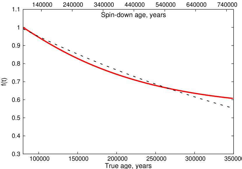
Figure 4: Magnetic field decay derived from the analysis of the sample of normal PSRs from the ATNF catalogue. The solid line corresponds to the reconstructed decay function, and the dashed line is an exponential fit. On the bottom horizontal axis we show the true (statistical) age, while the spin-down age is indicated on the top horizontal. The reconstructed law of the field evolution is corrected for the systematic error (see the text).

The original method was proposed by [Vivekanand & Narayan (1981)] and developed in [Narayan & Ostriker (1990)]. A recent discussion can be found in [(Vranešević & Melrose 2011)]. The basic idea is the following. Normally, the spin-down age of PSRs, $\tau$, increases (we do not consider young sources, for which magnetic field emergence can be important, see [Bernal et al. 2013, Popov & Turolla 2012b] and references therein). This happen due to spin-down and effective magnetic field evolution. If there is no evolution of effective magnetic fields then the number of pulsars with spin-down age less than some $\tau_{1}$ should be the same as the number of pulsars with true age less then $\tau_{1}-\overline{\tau}_{0}$, where $\overline{\tau}_{0}$ is the average initial spin-down age for the ensemble under study. This statement should be valid for any $\tau_{1}\gg\overline{\tau}_{0}$. The true age can be statistically estimated, and so we have a function $t$ vs. $\tau$. When this estimate is done, we can check if the assumption of constant field is valid.

We reconstruct the function $t$ vs. $\tau$ for spin-down ages $\sim 10^{5}$ – $10^{6}$ yrs and use it to estimate the rate of field decay in the framework of magneto-dipole spin-down with evolving field. To derive $t$ – $\tau$ from the observational data we make some assumptions. At first, we use the range of spin-down ages in which selection effects are not very important (this assumption is checked by comparison of cumulative distance distributions for sources of different ages; this assumption is mainly related to the upper limit of the range). Then we assume that PSRs have some maximum spin-down age at birth (i.e., initial positions of PSRs in the $p$-$\dot{p}$ diagram are confined in some limited region), it determines the lower limit of the range of spin-down ages used in our approach. Finally, we assume that the birthrate of PSRs is constant. The latter assumption allows us to introduce a “statistical age”, $t_{\mathrm{stat}}=N(\tau)/NSBR$, where $N(\tau)$ is the number of PSRs with spin-down ages below a given value, and $NSBR$ is an internal parameter of the model which corresponds to the birth rate of NSs used for our estimates of field decay. We use $t_{\mathrm{stat}}$ as an estimate of the true age of a PSR. So, the subscript is dropped in the following.

The determination of $NSBR$ is related to the maximum spin-down age at birth, $\tau_{0}$. We assume that for this value $t_{\mathrm{stat}}$ and $\tau$ are equal, so $NSBR=N(\tau_{0})/\tau_{0}$. This value is different from the actual total birth rate of NSs.

After we are able to reconstruct from observations (or using data from a synthetic model) the dependence $t$-$\tau$, we use it to derive the function, $f(t)$, which describes the field decay. It is assumed that the field is only diminishing:

$$B(t)=B_{0}f(t).$$ (2)

In Fig.3 we show results in which as input data we used population synthesis calculations with constant magnetic field. There is some systematic error, and there is some variance due to limited statistics, however, the method successfully reconstructs the field behaviour. The systematic error was studied in details using population synthesis modeling where the law of magnetic field evolution is known. We are able to correct our results to reduce this systematics.

Then we apply our method to real data from Parkes and Swinburne surveys. Results are given in Fig.4. Our calculations demonstrate that the field is decaying for the spin-down age range $8\times 10^{4}$–$10^{6}$ yrs (corresponding to the true age range $8\times 10^{4}$–$3.5\times 10^{5}$ yrs). The decay function can be fitted with an exponential with time scale $4.6\times 10^{5}$ yrs (Igoshev et al., in preparation). The rate of decay is compatible with the Hall time scale in normal pulsars.

4 Discussion

In this section we present several GUNS-related issues, which provide links with other types of sources, not discussed above. Still, all of them a related to the evolution with changing magnetic field.

4.1 “One second” problem

Here we present and discuss new unpublished results, related to the unified description of the NS population in the framework of decaying magnetic field.

When one is developing such general approach as GUNS, it is very important to use as many ways to compare calculations with observations as possible. Confronting modeled data with additional observed parameters can bring new questions, new problems, and in this subsection we are going to discuss one.

In ([Popov et al. 2010]) the authors were able to explain numbers of observed sources of different kind (PSRs, magnetars, M7) using one framework. Some assumptions used in these calculations are now independently verified. Unique initial spin period distribution for different NSs is supported with the data on NSs in SNRs (Sec. 2). The existence of moderate field decay in normal pulsars is confirmed (Sec. 3). On the other hand, field is not decaying much on the time scale $1-10$ Myrs (Sec. 4.2). However, more detailed comparison with the data shows, that, probably, further improvements in the model are necessary.

Speaking about close-by cooling NSs (M7 and PSRs) observed by ROSAT we can look at their current distribution in the $p$-$\dot{p}$ diagram. Observed sources are divided into two well-separated groups: standard field PSRs with $p\lesssim 0.3$ s and M7 with larger $\dot{p}$ and with $p\gtrsim 3$ s. Calculations provided quite a different picture. In Fig.5 we present preliminary results for the data set similar to that used in ([Popov et al. 2010]), and confront them with the observational data. The synthetic distribution is smooth. Sources with $p\sim 1$ s are predicted, but are not observed.

Several explanations can be proposed. The first is obvious: we have very low observational statistics. Still, the fact that sources in different peaks belong to different subpopulation of NSs is against it. The second explanation is related to unmodeled (and unknown) selection effects. Indeed, the underlying distribution can be smooth (as predicted by the model), but in observations we see two separated groups. However, preliminary analysis of possible effects does not allow us to fit the data (Popov, in prep.). Finally, it is possible that the model needs modifications (for example, cooling of NSs with low and standard magnetic fields can be finetuned to make contribution of such sources larger). At the moment, we think that this option is the most probable, and new calculations are in progress.

Joint description of the magneto-rotational and cooling evolution of NSs of all types in one population synthesis model would be the final step for GUNS. But it seems that several important issues are not clear, yet.

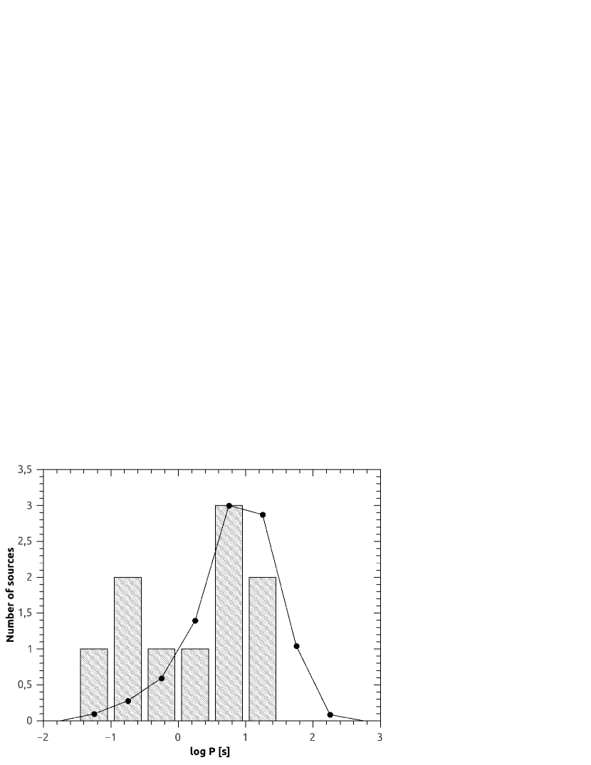
Figure 5: Spin period distribution for close-by cooling NSs. The histogram corresponds to the observed sources. Two maxima (PSRs and M7) are clearly visible. The solid line with symbols shows the results of calculations (Popov, in preparation).

4.2 High-mass X-ray binaries and NS evolution

GUNS cannot be limited to isolated NSs alone. Binaries inevitably have to be included. This can be tackled from two sides. First, some types of binaries are excellent test beds for NS evolution. Second, if we have at least some general ideas about GUNS, then we can use them to explain properties of peculiar sources in binaries. In this subsection we give examples for both approaches.

Magnetic field evolution is normally tested using data on PSRs and magnetars. This means that for highly magnetized NSs we cannot confront predictions vs. observations on a time scale larger than few tens or hundreds thousand years. High-mass X-ray binaries (HMXBs) give an opportunity to solve this problem. NSs in these systems have ages $\gtrsim$1–10 Myrs. Since accretion normally is due to stellar wind, the accretion rate is not very high and duration of the accretion stage is not very long, so the field is not much influenced by it. Determination of magnetic fields is possible in rare cases directly via cyclotron line observation. But mostly fields can be estimated using known spin periods and their variations.

Several methods of magnetic field estimation in X-ray pulsars were applied by [Chashkina & Popov (2012)]. Among them the authors used a new model of quasi-spherical accretion by [Shakura et al. (2012)]. Application of this model allowed to demonstrate that magnetic field distribution in HMXBs is compatible with predictions of the scenario by the Alicante group (see, for example, [Aguilera et al. 2008]). For standard-value fields the distribution of NSs in HMXBs is similar to that of PSRs, i.e. no additional significant decay happens during lifetime of HMXBs. We think that HMXBs can be fruitfully used for further comparison of the GUNS prediction with observational data.

Now, we briefly illustrate how standard ingredients of GUNS can be used to explain properties of peculiar sources in binary systems. We do this by looking at SXP1062 — a recently discovered X-ray binary in the SMC.

The unique feature of SXP1062 is its association with a SNR. This provides an estimate for the age of the NS in this system, $\sim(2$–$4)\times 10^{4}$ yrs ([Haberl et al. 2012, Hénault-Brunet et al. 2012]). If we assume that the source is close to spin equilibrium (new observations support it, [Sturm et al. 2013]), then the present day field is $\sim 10^{13}$ G. With such short age it is difficult to come to the stage of accretion and spin-down the NS to 1062 s period. There are two possibilities. The first, proposed by [Haberl et al. 2012], is related to long initial spin period: $p_{0}\sim 1$s. The second, proposed by [Popov & Turolla (2012c)], is related to the magnetic field decay. If the latter possibility is realized, then SXP1062 is an evolved magnetar in a HMXB system — the first example of such a source.

4.3 Buried and resurrected

A scenario for GUNS includes the possibility that magnetic field can be initially buried by intensive fall-back accretion, and then the field emerges on a timescale $\lesssim 10^{4}$–$10^{5}$ yrs ([Muslimov & Page, Ho 2011]). In this subsection we briefly discuss several cases in which this process can be important.

The bestiary of NSs is continuously enriched with new monsters. A NS in the SNR Kes 79 was proposed to be a buried magnetar ([Shabaltas & Lai 2012]). If this is the case, we have to find a place for this object in the GUNS. Moreover, similar sources can give a clue to the formation mechanisms of magnetars ([Popov 2013]).

The spin period of this source is 0.105 s. The period derivative is small, so the present inferred dipole field is low. However, large pulse fraction points to large crustal field ([Shabaltas & Lai 2012]). If the field was rapidly buried during the first minutes or hours after the NS formation (as the standard scenario predicts), then the present day spin period is very close to the initial one. The value 0.105 s is in contradiction with the standard mechanism of field generation in magnetars ([Duncun & Thompson 1992]). Two possibilities can be discussed. Either, in Kes79 we have a true magnetar, and so the dynamo mechanism is not valid. Or, the object in Kes 79 is somehow different from normal magnetars (maybe, belonging to low-field magnetars, see [Turolla & Esposito 2013]), the dipole magnetic field of which are not too large at birth). Discovery of a similar object, but with a millisecond period, would be a proof for the standard Duncan-Thompson scenario.

CCOs with low-fields (the so-called anti-magnetars) are believed to be objects with buried magnetic fields. Do we have other evidence in favour of buried and emerging field? In our opinion, two observations can be made to support this picture ([Popov & Turolla 2012b]).

The first is related to close-by cooling NSs. As it was noted already, there are two sub-populations among these sources: PSRs and M7. Detailed modeling also shows that there is no necessity to add more sources of different nature. However, in SNRs we see that a significant fraction of sources belong to CCOs. If so, we expect to see matured CCOs around us as thermal X-ray sources. Their absence provides an indirect argument in favour of the hypothesis that such objects “disappear” on a time scale $\lesssim 10^{5}$ yrs due to field emergence. I.e., probably there are matured CCOs in the solar vicinity observed as soft sources, but we do not recognize them.

For the second we have return to HMXBs. Again, if anti-magnetars form a significant fraction of young NSs, then we expect to find them in HMXBs, unless something happens. There are no confirmed NSs with low magnetic fields in HMXBs. This also can be considered as an indirect argument in favour of emerging magnetic field.

Finally, the difference between initial spin period distributions derived by [Popov & Turolla (2012a)] and [Noutsos et al. (2013)] can also be explained by emerging magnetic field. NSs from the “tail” in [Noutsos et al. (2013)] could be absent in the younger sample by [Popov & Turolla (2012a)]. Simply, sources visible in the older population in the “tail” could be “hidden” by fall-back in their early ages.

4.4 Alignment

Often when we discuss magnetic fields of NSs (especially, in the context of magneto-rotational evolution) we mean effective field, which includes also the angle between spin and dipole axis. Evolution of this angle towards the position of smaller energy losses can mimic magnetic field decay. Probably, this is one of the most elusive (luckily, also one of the least important) ingredient of GUNS.

Potentially, HMXBs can be used to measure the angle and to put limit on its evolution (as they can be used to test field evolution on the time scale $\gtrsim 1$ – $10$ Myrs). A preliminary analysis ([Karino 2007]) shows that angles are not close to 0 or 90 degrees in sources with average ages about few Myrs, which, in our opinion, excludes significant evolution of the angle on shorter (pulsar life time) time scales. Additionally, in the early version of a compilative Be/X-ray binaries catalogue ([Popov & Raguzova 2004]) we look for correlation of pulse fraction with other parameters of the sources. Nothing was found, and potentially this argues against significant angle evolution towards one of limiting positions. Future theoretical studies which include detailed models for pulse shape are necessary.

4.5 Isolated accretors

A major step in understanding of NSs will be taken when really old isolated objects are discovered. Probably, the unique possibility to do it is to find isolated accreting NSs. This will allow us to test models on a time scale $\sim$ few Gyrs.

Accreting isolated NSs have been discussed since early 70s. Some hopes to detect them were related to ROSAT (see a review in [Treves et al. 2000]). Then it was shown that in a standard (at that moment) evolutionary scenario NSs mostly do not reach the stage of accretion from the interstellar medium ([Popov et al. 2000]). However, modern scenario makes predictions slightly more optimistic.

[Boldin & Popov (2010)] used analytical approximations to the evolutionary scenario from ([Aguilera et al. 2008]) to model NS evolution on a long time scale. It was shown that NSs with initially large magnetic fields are able to reach the stage of accretion. Funny thing about it is the following. Despite optimistic predictions in early 90s, no accreting isolated NSs were discovered. Instead, unpredicted cooling NSs (M7) were found. But exactly these sources in future may become isolated accretors, and if there are accreting isolated NSs around us most probably they were M7-like when they were young!

Discovery of old (accreting) isolated NSs is very important for GUNS. This is a task for future surveys in soft X-rays, for example for eROSITA onboard Spectrum-X-Gamma, which can also contribute to young NSs studies.

5 Conclusions

During the last several years the zoo of young isolated NSs started to look not so unexplainably motley. Some evolutionary links between different types of sources are established, and more are coming with the help of the concept of emerging magnetic field. Different approaches to model and interpret data can help to probe various assumptions, as it probably happened with the initial spin period distribution. Diverse methods to confront model predictions with observations are necessary, because evolutionary scenarios now have too many ingredients and free parameters. Inclusion of HMXBs in these considerations can be fruitful in many respects, especially probing magnetic field and spin-dipole angle evolution. Discoveries of isolated NSs beyond magnetar, radio pulsar, and residual thermal emission stages is very much welcomed.