Van der Waals Coefficients for the Alkali-metal Atoms in the Material Mediums

Abstract

The damping coefficients for the alkali atoms are determined very accurately by taking into account the optical properties of the atoms and three distinct types of trapping materials such as Au (metal), Si (semi-conductor) and vitreous SiO₂ (dielectric). Dynamic dipole polarizabilities are calculated precisely for the alkali atoms that reproduce the damping coefficients in the perfect conducting medium within 0.2% accuracy. Upon the consideration of the available optical data of the above wall materials, the damping coefficients are found to be substantially different than those of the ideal conductor. We also evaluated dispersion coefficients for the alkali dimers and compared them with the previously reported values. These coefficients are fitted into a ready-to-use functional form to aid the experimentalists the interaction potentials only with the knowledge of distances.

Accurate information on the long-range interactions such as dispersion (van der Waals) and retarded (Casimir-Polder) potentials between two atoms and between an atom and surface of the trapping material are necessary for the investigation of the underlying physics of atomic collisions especially in the ultracold atomic experiments lifshitzbook ; casimir1 ; london ; israel . Presence of atom-surface interactions lead to a shift in the oscillation frequency of the trap which alters the trapping frequency as well as magic wavelengths for state-insensitive trapping of the trapped condensate. Moreover, this effect has also gained interest in generating novel atom optical devices known as the “atom chips”. In addition, the knowledge of dispersion coefficients is required in experiments of photo-association, fluorescence spectroscopy, determination of scattering lengths, analysis of feshbach resonances, determination of stability of Bose-Einstein condensates (BECs), probing extra dimensions to accommodate Newtonian gravity in quantum mechanics etc. roberts ; amiot ; leo ; harber ; leanhardt ; lin .

There have been many experimental evidences of an attractive force between neutral atoms and between neutral atoms with trapping surfaces but their precise determinations are relatively difficult. In the past two decades, several groups have evaluated dispersion coefficients $C_{3}$ defining interaction between an atom and a wall using various approaches derevianko1 ; derevianko4 ; jiang without rigorous estimate of uncertainties. More importantly, they are evaluated for a perfect conducting wall which are quite different from an actual trapping wall. Since these coefficients depend on the dielectric constants of the materials of the wall, therefore it is worth determining them precisely for trapping materials with varying dielectric constants (for good conducting, semi conducting, and dielectric mediums) as has been attempted in lach1 ; caride . Casimir and Polder casimir1 had estimated that at intermediately large separations the retardation effects of the virtual photons passing between the atom and its image weakens the attractive atom-wall force and the force scales with a different power law (given in details below). In this paper, we carefully examine these retardation or damping effects which have not been extensively studied earlier. We also parameterized our damping coefficients into a readily usable form to be used in experiments.

The atom-surface interaction potential resulting from the fluctuating dipole moment of an atom interacting with its image in the surface is formulated by lifshitzbook ; lach1

$$U^{a}(R)=-\frac{\alpha_{fs}^{3}}{2\pi}\int_{0}^{\infty}d\omega\omega^{3}\alpha(\iota\omega)\int_{1}^{\infty}d\xi e^{-2\alpha_{fs}\xi\omega R}H(\xi,\epsilon(\iota\omega)),$$ (1)

where $\alpha_{fs}$ is the fine structure constant, $\epsilon(\omega)$ is the frequency dependent dielectric constant of the solid, $R$ is the distance between the atom and the surface and $\alpha(\iota\omega)$ is the ground state dynamic polarizability with imaginary argument. The function $H(\xi,\epsilon(\iota\omega))$ is given by

$$H(\xi,\epsilon)=(1-2\xi^{2})\frac{\sqrt{\xi^{2}+\epsilon-1}-\epsilon\xi}{\sqrt{\xi^{2}+\epsilon-1}+\epsilon\xi}+\frac{\sqrt{\xi^{2}+\epsilon-1}-\xi}{\sqrt{\xi^{2}+\epsilon-1}+\xi}$$

with the Matsubara frequencies denoted by $\xi$.

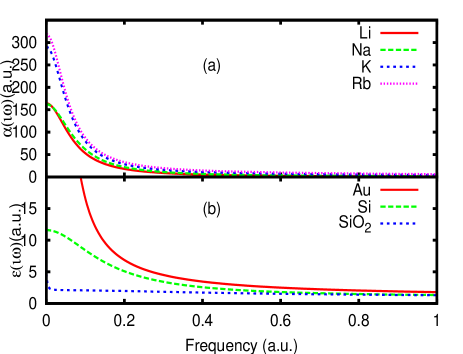
Figure 1: Dynamic polarizabilities of the Li, Na, K and Rb atoms and dielectric permittivity of the Au, Si and SiO₂ surfaces along the imaginary axis as functions of frequencies.

In asymptotic regimes, the Matsubara integration is dominated by its first term and the potential can be approximated to $U^{a}(R)=-\frac{C_{3T}}{R^{3}}$ with $C_{3T}=\frac{\alpha(0)}{4}(\epsilon(0)-1)/(\epsilon(0)+1)$. The potential form can be described more accurately at the retardation distances as $U^{a}(R)=-\frac{C_{4}}{R^{4}}$ and at the non-retarded region as $U^{a}(R)=-\frac{C_{3}}{R^{3}}$ casimir1 . To express the potential in the intermediate region, these approximations are usually modified either to $U^{a}(R)=-\frac{C_{4}}{(R+\lambdabar)R^{3}}$ or to $U^{a}(R)=-\frac{C_{3}}{R^{3}}f_{3}(R)$ where $\lambdabar$ and $f_{3}(R)$ are respectively known as the reduced wavelength and damping function. It would be interesting to testify the validity of both the approximations by evaluating $C_{3}$, $C_{4}$ and $f_{3}(R)$ coefficients together for different atoms in conducting, semi-conducting and dielectric materials. Since the knowledge of magnetic permeability of the material is required to evaluate $C_{4}$ coefficients, hence we determine only the $C_{3}$ and $f_{3}(R)$ coefficients. With the knowledge of $C_{3}$ and $f_{3}$ values, the atom-surface interaction potentials can be easily reproduced and they can be generalized to other surfaces.

Table 1: Calculated $C_{3}$ coefficients along with their uncertainties for the alkali-metal atoms and their comparison with other reported values. Classification of various contributions are in accordance with derevianko1 ^a, derevianko4 ^b and kharchenko ^c.

	Li	Na	K	Rb
Perfect Conductor
Core	0.074	0.332	0.989	1.513
Valence	1.387	1.566	2.115	2.254
Core-Valence	$\sim 0$	$\sim 0$	$-0.016$	$-0.028$
Tail	0.055	0.005	0.003	0.003
Total	1.516(2)	1.904(2)	3.090(4)	3.742(5)
Others	1.5178 a	1.8858b	2.860b	3.362b
		1.889c
Metal: Au
Core	0.010	0.051	0.263	0.419
Valence	1.160	1.285	1.804	1.927
Core-Valence	$\sim 0$	$\sim 0$	-0.005	-0.010
Tail	0.029	0.002	0.001	0.002
Total	1.199(2)	1.338(1)	2.062(4)	2.338(4)
Others lach1	1.210	1.356	2.058	2.79
Semi-conductor: Si
Core	0.006	0.033	0.184	0.299
Valence	0.993	1.099	1.543	1.649
Core-Valence	$\sim 0$	$\sim 0$	-0.004	-0.008
Tail	0.023	0.002	0.001	0.001
Total	1.022(2)	1.134(1)	1.724(3)	1.942(4)
Dielectric: SiO2
Core	0.004	0.022	0.116	0.184
Valence	0.468	0.519	0.726	0.775
Core-Valence	$\sim 0$	$\sim 0$	-0.002	-0.004
Tail	0.012	0.001	0.001	0.001
Total	0.4844(8)	0.5424(5)	0.839(1)	0.956(2)

In general, the $C_{3}$ coefficient is given by

$$C_{3}\approx\frac{1}{4\pi}\int_{0}^{\infty}d\omega\alpha(\iota\omega)\frac{\epsilon(\iota\omega)-1}{\epsilon(\iota\omega)+1}.$$ (2)

For a perfect conductor $\epsilon\rightarrow\infty$, $\frac{\epsilon(\iota\omega)-1}{\epsilon(\iota\omega)+1}\rightarrow 1$ and for other materials with their refractive indices $n=\sqrt{\epsilon}$ varying between 1 and 2, $\frac{\epsilon(\iota\omega)-1}{\epsilon(\iota\omega)+1}\approx\frac{\epsilon(0)-1}{\epsilon(0)+1}$ is nearly a constant and can be approximated to 0.77. For more preciseness, it is necessary to consider the actual frequency dependencies of $\epsilon$s in the materials. In the present work, three distinct materials such as Au, Si and SiO₂ belonging to conducting, semi-conducting and dielectric objects respectively, are taken into account to find out $f_{3}(R)$ functions and compared against a perfect conducting wall for which case we express kharchenko

$$f_{3}(R) = \frac{1}{4\pi C_{3}}\int_{0}^{\infty}d\omega\alpha(\iota\omega)e^{-2\alpha_{fs}\omega R}Q(\alpha_{fs}\omega R),$$ (3)

with $Q(x)=2x^{2}+2x+1$. To find out $f_{3}(R)$ for the other surfaces, we evaluate $U^{a}(R)$ by substituting their $\epsilon(\iota\omega)$ values in Eq. (1).

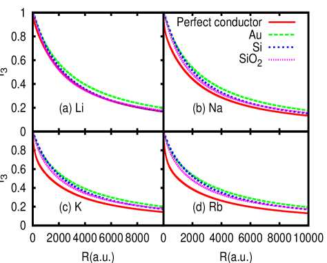
Figure 2: The retardation coefficient $f_{3}$(R) (dimensionless) for Li, Na, K and Rb as a function of atom-wall distance R.

Similarly, the leading term in the long-range interaction between two atoms denoted by $a$ and $b$ is approximated by $U^{ab}(R)=-\frac{C_{6}^{ab}}{R^{6}}$, where the $C_{6}^{ab}$ is known as the van der Waals coefficient and $R$ is the distance between two atoms. If retardation effects are included then it is modified to $U^{ab}(R)=-\frac{C_{6}^{ab}}{R^{6}}f_{6}^{ab}(R)$. The dispersion coefficient $C_{6}^{ab}$ and the damping coefficient $f_{6}^{ab}(R)$ between the atoms can be estimated using the expressions kharchenko

$$C_{6}^{ab} = \frac{3}{\pi}\int_{0}^{\infty}d\omega\alpha^{a}(\iota\omega)\alpha^{b}(\iota\omega),\ \ \ \ \text{and}$$

$$f_{6}^{ab} = \frac{1}{\pi C_{6}^{ab}}\int_{0}^{\infty}d\omega\alpha^{a}(\iota\omega)\alpha^{b}(\iota\omega)e^{-2\alpha_{fs}\omega R}P(\alpha_{fs}\omega R),$$

where $P(x)=x^{4}+2x^{3}+5x^{2}+6x+3$.

Table 2: Fitting parameters $a$ and $b$ for $f_{3}$ coefficients with a perfectly conducting wall, Au, Si, and SiO₂ surfaces.

	Li	Na	K	Rb
Perfect Conductor
a	0.9843	1.0802	1.1845	1.2598
b	0.0676	0.0866	0.0808	0.0907
Metal: Au
a	0.9775	0.9846	1.0248	1.0437
b	0.0675	0.0614	0.0532	0.0558
Semi-conductor: Si
a	0.9436	0.9436	0.9749	0.9869
b	0.0638	0.0718	0.0622	0.0647
Dielectric: SiO2
a	0.9754	0.9789	1.0238	1.0423
b	0.0650	0.0746	0.0649	0.0685

Using our previously reported E1 matrix elements arora-sahoo1 ; arora-sahoo2 and experimental energies, we plot the dynamic polarizabilities of the ground states in Fig. 1 of the considered alkali atoms. The static polarizabilities corresponding to $\omega=0$ come out to be 164.1(7), 162.3(2), 289.7(6) and 318.5(8), as given in arora-sahoo1 ; arora-sahoo2 , against the experimental values 164.2(11) li-exp , 162.4(2) na-exp , 290.58(1.42) k-exp and 318.79(1.42) k-exp in atomic unit (a.u.) for Li, Na, K and Rb atoms respectively. It clearly indicates the preciseness of our estimated results. The main reason for achieving such high accuracies in the estimated static polarizabilities is due to the use of E1 matrix elements extracted from the precise lifetime measurements of few excited states and by fitting our E1 results obtained from the relativistic coupled-cluster calculation at the singles, doubles and partial triples excitation level (CCSD(T) method) to the measurements of the static polarizabilities of the excited states.

Table 3: $C_{6}$ coefficients with fitting parameters for the alkali dimers. Contributions from the valence, core and valence-core polarizabilities alone are labeled as $C_{6}^{v}$, $C_{6}^{c}$ and $C_{6}^{vc}$, respectively and $C_{6}^{ct}$ corresponds to contributions from the remaining cross terms. References: ^aderevianko5 , ^bmarinescu , ^cmitroy1 , ^dsahooli , ^erussier , ^fpashov , ^gchin .

Dimer	$C_{6}^{v}$	$C_{6}^{c}$	$C_{6}^{vc}$	$C_{6}^{ct}$	$C_{6}$(Total   )	Others	Exp	a	b
Li-Li	1351	0.07	$\sim$ 0	39	1390(4)	1389(2)a,1388b,1394.6c ,1473d		0.8592	0.0230
Li-Na	1428	0.32	$\sim$ 0	37	1465(3)	1467(2)a		0.8592	0.0245
Li-K	2201	1.27	$\sim$ 0	119	2321(6)	2322(5)a		0.8640	0.0217
Li-Rb	2368	1.94	$\sim$ 0	179	2550(6)	2545(7)a		0.8666	0.0262
Na-Na	1515	1.51	$\sim$ 0	33	1550(3)	1556(4)a, 1472b,1561c		0.8591	0.0262
Na-K	2316	6.24	$\sim$ 0	118	2441(5)	2447(6)a	2519e	0.8555	0.0231
Na-Rb	2490	9.60	$\sim$ 0	184	2684(6)	2683(7)a		0.8686	0.0232
K-K	3604	29.89	0.01	261	3895(15)	3897(15)a, 3813b,3905c	3921f	0.8738	0.0207
K-Rb	3880	46.91	0.02	465	4384(12)	4274(13)a		0.8738	0.0207
Rb-Rb	4178	73.96	0.4	465	4717(19)	4691(23)a, 4426b,4635c	4698g	0.8779	0.0207

Substituting the dynamic polarizabilities in Eq. (2), we evaluate the $C_{3}$ coefficients for a perfect conductor (to compare with previous studies), for a real metal Au, for a semi conductor object Si and for a dielectric substance of glassy structure SiO₂. These values are given in Table 1 with break down from various individual contributions and estimated uncertainties are quoted in the parentheses after ignoring errors from the used experimental data. To achieve the claimed accuracy in our results it was necessary to use the complete tabulated data for the refraction indices of Au, Si, and SiO₂ to calculate their dielectric permittivities at all the imaginary frequencies palik . We evaluate the imaginary parts of the dielectric constants using the relation $\rm{Im}\left(\epsilon(\omega)\right)=2n(\omega)\kappa(\omega)$, where n and $\kappa$ are the real and imaginary parts of the refractive index of a material. The available data for Si and SiO₂ are sufficiently extended to lower frequencies. However, they are extended to the lower frequencies for Au with the help of the Drude dielectric function caride

$$\epsilon(\omega)=1-\frac{\omega_{p}^{2}}{\omega(\omega+\iota\gamma)},$$ (4)

with relaxation frequency $\gamma=0.035$ eV and plasma frequency $\omega_{p}=9.02$ eV. The corresponding real values at imaginary frequencies are obtained by using the Kramers-Kronig formula

$$\rm{Re}(\epsilon(\iota\omega))=1+\frac{2}{\pi}\int_{0}^{\infty}d\omega^{\prime}\frac{\omega^{\prime}\rm{Im}(\epsilon(\omega^{\prime}))}{\omega^{2}+{\omega^{\prime}}^{2}}.$$ (5)

In bottom part of Fig. 1, the $\epsilon(\iota\omega)$ values as a function of imaginary frequency are plotted for Au, Si, and SiO₂. The behavior of $\epsilon(\iota\omega)$ for various materials is obtained as expected and they match well with the graphical representations given by Caride and co-workers caride .

As shown in Table 1, $C_{3}$ coefficients increase with the increase in atomic mass. First we present our results for the $C_{3}$ coefficients for the interaction of these atoms with a perfectly conducting wall. The dominant contribution to the $C_{3}$ coefficients is from the valence part of the polarizability. We also observed that the core contribution to the $C_{3}$ coefficients increases with the increasing number of electrons in the atom which is in agreement with the prediction made in Ref. derevianko4 . Our results are also in good agreement with the results reported by Kharchenko et al. kharchenko for Na. Therefore, our results obtained for other materials seem to be reliable enough. We noticed that the $C_{3}$ coefficients for a perfect conductor were approximately 1.5, 2, and 3.5 times larger than the $C_{3}$ coefficients for Au, Si, and SiO₂ respectively. The decrease in the coefficient values for the considered mediums can be attributed to the fact that in case of dielectric material the theory is modified for non-unity reflection and for different origin of the transmitted waves from the surface. In addition to this, for Si and SiO₂ there are additional interactions due to charge dangling bonds specially at shorter separations. The recent estimations with Au medium carried out by Lach et al. lach1 are in agreement with our results since the polarizability database they have used is taken from Ref. derevianko4 . These calculations seem to be sensitive on the choice of grids used for the numerical integration. An exponential grid yield the results more accurately and it is insensitive to choice of the size of the grid in contrast to a linear grid. In fact with the use of a linear grid having a spacing $0.1$, we observed a 3-5% fall in $C_{3}$ coefficients for the considered atoms. The reason being that most of the contributions to the evaluation of these coefficients come from the lower frequencies which yield inaccuracy in the results for large grid size.

Fig. 2 shows a comparison of the $f_{3}(\text{R})$ values obtained for Li, Na, K, and Rb atoms as a function of atom-wall separation distance R for the four different materials studied in this work. As seen in the figure, the retardation coefficients are the smallest for an ideal metal. At very short separation distances the results for a perfectly conducting material differs from the results of Au, Si, and SiO₂ by less than 4%. As the atom-surface distance increases, the deviations of $f_{3}$ results for various materials from the results of an ideal metal are considerable and vary as 18%, 15% and 6% for Li; 33%, 14% and 18% for Na; 40%, 13% and 26% for K; and 50%, 13% and 33% for Rb in Au, Si, and SiO₂ surfaces respectively. The deviation of results between an ideal metal and other dielectric surfaces is smallest for the Li atom and increases appreciably for the Rb atom. We use the functional form to describe accurately the atom-wall interaction potential at the separate distance R as

$$f_{3}(R)=\frac{1}{a+b(\alpha_{fs}R)}.$$ (6)

By extrapolating data from the above figure, we list the extracted $a$ and $b$ values for the considered atoms in all the materials in Table 2.

In Table 3, we present our calculated results for the $C_{6}$ coefficients for the alkali dimers. In columns II, III and IV, we give individual contributions from the valence, core and valence-core polarizabilities to $C_{6}$ evaluation and column V represents contributions from the cross terms which are found to be crucial for obtaining accurate results. As can be seen from Table 1, the trends are almost similar to $C_{3}$ evaluation. A comparison of our $C_{6}$ values with other recent calculations and available experimental results is also presented in the same table. Using the similar fitting procedure as for $f_{3}$, we obtained fitting parameters $a$ and $b$ for $f_{6}$ from Fig. 3 which are quoted in the last two columns of the above table.

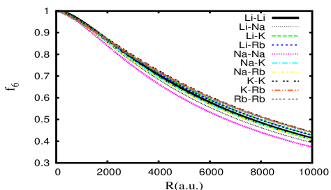
Figure 3: The retardation coefficient $f_{6}$(R) (dimensionless) for the alkali dimers as a function of atom-atom distance R.

To summarize, we have investigated the dispersion and damping coefficients for the atom-wall and atom-atom interactions for the Li, Na, K, and Rb atoms and their dimers in this work. The interaction potentials of the alkali atoms are studied with Au, Si, and SiO₂ surfaces and found to be very different than a perfect conductor. It is also shown that the interaction of the atoms in these surfaces is considerably distinct from each other. A readily usable functional form of the retardation coefficients for the interaction between two alkali atoms and alkali atom with the above mediums is provided. Our fit explains more than 99% of total variation in data about average. The results are compared with the other theoretical and experimental values.

The work of B.A. is supported by the CSIR, India (Grant no. 3649/NS-EMRII). We thank Dr. G. Klimchitskaya and Dr. G. Lach for some useful discussions. B.A. also thanks Mr. S. Sokhal for his help in some calculations. Computations were carried out using 3TFLOP HPC Cluster at Physical Research Laboratory, Ahmedabad.

References

- (1) E. M. Lifshitz and L. P Pitaevskii, Statistical Physics, Pergamon Press, Oxford, London (1980).
- (2) H. B. G. Casimir and D. Polder, Phys. Rev. 73, 4 (1948).
- (3) F. London, Z. Physik 63, 245 (1930).
- (4) J. Israelachvili, Intermolecular and Surface Forces, Academic Press, San Diego (1992).
- (5) J. L. Roberts et al., Phys. Rev, Lett. 81, 5109 (1998).
- (6) C. Amiot and J. Verges, J. Chem. Phys. 112, 7068 (2000).
- (7) P. J. Leo, C. J. Williams and P. S. Julienne, Phys. Rev. Lett. 85, 2721 (2000).
- (8) D. M. Harber et al., J. Low Temp. Phys. 133, 229 (2003).
- (9) A. E. Leanhardt et al., Phys. Rev. Lett. 90, 100404 (2003).
- (10) Y. Lin et al., Phys. Rev. Lett. 92, 050404 (2004).
- (11) A. Derevianko, W. R. Johnson and S. Fritzsche, Phys. Rev. A 57, 2629 (1998).
- (12) A. Derevianko et al., Phys. Rev. Lett. 82, 3589 (1999).
- (13) J. Jiang, Y. Cheng and J. Mitroy, J. Phys. B 46, 125004 (2013).
- (14) G. Lach, M. Dekieviet and U. D. Jentschura, Int. J. Mod. Phys. A 25, 2337 (2010).
- (15) A. O. Caride et al., Phys. Rev. A 71, 042901 (2005).
- (16) P. Kharchenko, J. F. Babb and A. Dalgarno, Phys. Rev. A 55, 3566 (1997).
- (17) B. Arora and B. K. Sahoo, Phys. Rev. A 86, 033416 (2012).
- (18) B. K. Sahoo and B. Arora, Phys. Rev. A 87, 023402 (2013).
- (19) A. Miffre et al., Eur. Phys. J. D 38, 353 (2006).
- (20) C. R. Ekstrom et al., Phys. Rev. A 51, 3883 (1995).
- (21) W. F. Holmgren et al., Phys. Rev. A 81, 053607 (2010).
- (22) E. D. Palik, Handbook of Optical Constants of Solids, Academic Press, San Diego (1985).
- (23) A. Derevianko, J. F. Babb and A. Dalgarno, Phys. Rev. A 83, 052704 (2001).
- (24) M. Marinescu, H. R. Sadeghpour and A. Dalgarno, Phys. Rev. A 49, 982 (1994).
- (25) J. Mitroy and M. W. J. Bromley, Phys. Rev. A 68, 052714 (2003).
- (26) L. W. Wansbeek et al., Phys. Rev. A 78, 012515 (2008); Erratum: Phys. Rev. A 82, 029901 (2010)
- (27) I. Russier-Antoine et al., J. Phys. B 33, 2753 (2000).
- (28) A. Pashov et al., Eur. Phys. J. D 46, 241 (2008).
- (29) C. Chin et al., Phys. Rev. A 70, 032701 (2004).