Optimal sparse volatility matrix estimation for high-dimensional Itô processes with measurement errors

Abstract

Stochastic processes are often used to model complex scientific problems in fields ranging from biology and finance to engineering and physical science. This paper investigates rate-optimal estimation of the volatility matrix of a high-dimensional Itô process observed with measurement errors at discrete time points. The minimax rate of convergence is established for estimating sparse volatility matrices. By combining the multi-scale and threshold approaches we construct a volatility matrix estimator to achieve the optimal convergence rate. The minimax lower bound is derived by considering a subclass of Itô processes for which the minimax lower bound is obtained through a novel equivalent model of covariance matrix estimation for independent but nonidentically distributed observations and through a delicate construction of the least favorable parameters. In addition, a simulation study was conducted to test the finite sample performance of the optimal estimator, and the simulation results were found to support the established asymptotic theory.

, and t1Supported in part by NSF Grants DMS-10-5635 and DMS-12-65203. t2Supported in part by NSF Career Award DMS-0645676 and NSF FRG Grant DMS-08-54975.

1 Introduction

Modern scientific studies in fields ranging from biology and finance to engineering and physical science often need to model complex dynamic systems where it is essential to incorporate internally or externally originating random fluctuations in the systems [Aït-Sahalia, Mykland and Zhang (2005), Mueschke and Andrews (2006) and Whitmore (1995)]. Continuous-time diffusion processes, or more generally, Itô processes, are frequently employed to model such complex dynamic systems. Data collected in the studies are treated as the processes observed at discrete time points with possible noise contamination. For example, the prices of financial assets are usually modeled by Itô processes, and the price data observed at high-frequencies are contaminated by market microstructure noise. In this paper we investigate estimation of the volatilities of the Itô processes based on noisy data.

Several volatility estimation methods have been developed in the past several years. For estimating a univariate integrated volatility, popular estimators include two-scale realized volatility [Zhang, Mykland and Aït-Sahalia (2005)], multi-scale realized volatility [Zhang (2006) and Fan and Wang (2007)], realized kernel volatility [Barndorff-Nielsen et al. (2008)] and pre-averaging based realized volatility [Jacod et al. (2009)]. For estimating a bivariate integrated co-volatility, common methods are the previous-tick approach [Zhang (2011)], the refresh-time scheme and realized kernel volatility [Barndorff-Nielsen et al. (2011)], the generalized synchronization scheme [Aït-Sahalia, Fan and Xiu (2010)] and the pre-averaging approach [Christensen, Kinnebrock and Podolskij (2010)]. Optimal volatility and co-volatility estimation has been investigated in the parametric or nonparametric setting [Aït-Sahalia, Mykland and Zhang (2005), Bibinger and Reiß (2011), Gloter and Jacod (2001a, 2001b), Reiß (2011) and Xiu (2010)]. These works are for estimating scalar volatilities or volatility matrices of small size. Wang and Zou (2010) and Tao et al. (2011) studied the problem of estimating a large sparse volatility matrix based on noisy high-frequency financial data. Fan, Li and Yu (2012) employed a large volatility matrix estimator based on high-frequency data for portfolio allocation. The large volatility matrix estimation is a high-dimensional extension of the univariate case. It can be also considered as a generalization of large covariance matrix estimation for i.i.d. data to volatility matrix estimation for dependent data with measurement errors. Despite recent progress on volatility matrix estimation, there has been remarkably little fundamental theoretical study on optimal estimation of large volatility matrices. Consistent estimation of large matrices based on high-dimensional data usually requires some sparsity, and the sparsity may naturally result from appropriate formulation of some low-dimensional structures in the high-dimensional data. For example, in large volatility matrix estimation with high-frequency financial data sparsity means that a relatively small number of market factors play a dominate role in driving volatility movements and capturing the market risk. In this paper we establish the optimal rate of convergence for large volatility matrix estimation under various matrix norms over a wide range of classes of sparse volatility matrices. We expect that our work will stimulate further theoretical and methodological research as well as more application orientated study on large volatility matrix estimation.

Specifically we consider the problem of estimating the sparse integrated volatility matrix for a $p$-dimensional Itô process observed with additive noises at $n$ equally spaced discrete time points. The minimax upper bound is obtained by constructing a new procedure through a combination of the multi-scale and threshold approaches and by studying its risk properties. We first construct a multi-scale volatility matrix estimator and show that its elements obey subGaussian tails with a convergence rate $n^{-1/4}$. Then we threshold the constructed estimator to obtain a threshold volatility matrix estimator and derive its convergence rate. The upper bound depends on $n$ and $p$ through $n^{-1/4}\sqrt{\log p}$.

A key step in obtaining the optimal rate of convergence is the derivation of the minimax lower bound for the high-dimensional Itô process with measurement errors. We succeed in establishing the risk lower bound in three steps. First we select a particular subclass of Itô processes with a zero drift and a constant volatility matrix so that the volatility matrix estimation problem becomes a covariance matrix estimation problem where the observed data are dependent and have measurement errors; second, take a special transformation of the observations to convert the problem into a new covariance matrix estimation problem where the observed data have no measurement errors and are independent but not identically distributed, with covariance matrices equal to the constant volatility matrix plus an identity matrix multiplying by a shrinking factor depending on the sample size $n$; third, adopt the minimax lower bound technique developed in Cai and Zhou (2012) for sparse covariance matrix estimation based on i.i.d. data to establish a minimax lower bound for independent but nonidentically distributed observations. The minimax lower bound matches the upper bound obtained by the new procedure up to a constant factor, and thus the upper bound is rate-optimal.

The volatility matrix estimation is closely related to large covariance matrix estimation which received lots of attentions recently in the literature. While the covariance matrix plays a key role in statistical analysis, its classic estimation procedures, like the sample covariance matrix estimator, may behave very poorly when the matrix size is comparable to or exceeds the sample size. To overcome the curse of dimensionality, various regularization techniques have been developed for estimation of large covariance matrices in recent years. Wu and Pourahmadi (2003) explored nonparametric estimation of large covariance matrices by local stationarity. Ledoit and Wolf (2004) proposed to boost diagonal elements and downgrade off-diagonal elements of the sample covariance matrix estimator. Huang et al. (2006) used a penalized likelihood method to estimate large covariance matrices. Yuan and Lin (2007) considered large covariance matrix estimation in a Gaussian graph model. Bickel and Levina (2008a, 2008b) developed regularization methods by banding or thresholding the sample covariance matrix estimator when the matrix size is comparable to the sample size. El Karoui (2008) employed a graph model approach to characterize sparsity and investigated consistent estimation of large covariance matrices. Fan, Fan and Lv (2008) utilized factor models for estimating large covariance matrices. Johnstone and Lu (2009) studied consistent estimation of leading principal components in principal component analysis. Lam and Fan (2009) established sparsistency and convergence rates for large covariance matrix estimation. Cai, Zhang and Zhou (2010) and Cai and Zhou (2012) studied minimax estimation of covariance matrices when both sample size and matrix size are allowed to go to infinity and derived optimal convergence rates for estimating decaying or sparse covariance matrices.

The rest of the paper proceeds as follows. Section 2 presents the model and the data and constructs volatility matrix estimators. Section 3 establishes the asymptotic theory under sparsity for the constructed matrix estimators as both sample size and matrix size go to infinity. Section 4 derives the minimax lower bound for estimating a large sparse volatility matrix and shows that the threshold volatility matrix estimator asymptotically achieves the minimax lower bound. Thus combining results in Sections 3 and 4 together, we establish the optimality for large sparse volatility matrix estimation. Section 5 features a simulation study to illustrate the finite sample performances of the volatility matrix estimators. To facilitate the reading we relegate all proofs to Section 6 and two Appendix sections, where we first provide the main proofs of the theorems in Section 6 and then collect additional technical proofs in the two appendices.

2 Volatility matrix estimation

2.1 The model set-up

Suppose that $\mathbf{X}(t)=(X_{1}(t),\ldots,X_{p}(t))^{T}$ is an Itô process following the model

$$d\mathbf{X}(t)=\bolds{\mu}_{t}\,dt+\bolds{\sigma}_{t}^{T}\,d\mathbf{B}_{t},\qquad t\in[0,1],$$ (1)

where stochastic processes $\mathbf{X}(t)$, $\mathbf{B}_{t}$, $\bolds{\mu}_{t}$ and $\bolds{\sigma}_{t}$ are defined on a filtered probability space $(\Omega,{\mathcal{F}},\{{\mathcal{F}}_{t},t\in[0,1]\},P)$ with filtration ${\mathcal{F}}_{t}$ satisfying the usual conditions, $\mathbf{B}_{t}$ is a $p$-dimensional standard Brownian motion with respect to ${\mathcal{F}}_{t}$, $\bolds{\mu}_{t}$ is a $p$-dimensional drift vector, $\bolds{\sigma}_{t}$ is a $p$ by $p$ matrix, and $\bolds{\mu}_{t}$ and $\bolds{\sigma}_{t}$ are assumed to be predictable processes with respect to ${\mathcal{F}}_{t}$.

We assume that the continuous-time process $\mathbf{X}(t)$ is observed with measurement errors only at equally spaced discrete time points; that is, the observed discrete data $Y_{i}(t_{\ell})$ obey

$$Y_{i}(t_{\ell})=X_{i}(t_{\ell})+\varepsilon_{i}(t_{\ell}),\qquad i=1,\ldots,p,t_{\ell}=\ell/n,\ell=1,\ldots,n,$$ (2)

where $\varepsilon_{i}(t_{\ell})$ are noises with mean zero.

Let $\bolds{\gamma}(t)=\bolds{\sigma}_{t}^{T}\bolds{\sigma}_{t}$ be the volatility matrix of $\mathbf{X}(t)$. We are interested in estimating the following integrated volatility matrix of $\mathbf{X}(t)$,

$$\bolds{\Gamma}=(\Gamma_{ij})_{1\leq i,j\leq p}=\int_{0}^{1}\bolds{\gamma}(t)\,dt=\int_{0}^{1}\bolds{\sigma}_{t}^{T}\bolds{\sigma}_{t}\,dt$$

based on noisy discrete data $Y_{i}(t_{\ell})$, $i=1,\ldots,p$, $\ell=1,\ldots,n$.

2.2 Estimator

Let $K$ be an integer and $\lfloor n/K\rfloor$ be the largest integer $\leq n/K$. We divide $n$ time points $t_{1},\ldots,t_{n}$ into $K$ nonoverlap groups $\bolds{\tau}^{k}=\{t_{\ell},\ell=k,K+k,2K+k,\ldots\}$, $k=1,\ldots,K$. Denote by $|\bolds{\tau}^{k}|$ the number of time points in $\bolds{\tau}^{k}$. Obviously, the value of $|\bolds{\tau}^{k}|$ is either $\lfloor n/K\rfloor$ or $\lfloor n/K\rfloor+1$. For $k=1,\ldots,K$, we write the $r$th time point in $\bolds{\tau}^{k}$ as $\tau_{r}^{k}=t_{(r-1)K+k}$, $r=1,\ldots,|\bolds{\tau}^{k}|$. With each $\bolds{\tau}^{k}$, we define the volatility matrix estimator

$$\tilde{\Gamma}_{ij}\bigl{(}\bolds{\tau}^{k}\bigr{)} = \sum_{r=2}^{|\bolds{\tau}^{k}|}\bigl{[}Y_{i}\bigl{(}\tau_{r}^{k}\bigr{)}-Y_{i}\bigl{(}\tau_{r-1}^{k}\bigr{)}\bigr{]}\bigl{[}Y_{j}\bigl{(}\tau_{r}^{k}\bigr{)}-Y_{j}\bigl{(}\tau_{r-1}^{k}\bigr{)}\bigr{]},$$

$$\tilde{\bolds{\Gamma}}\bigl{(}\bolds{\tau}^{k}\bigr{)} = \bigl{(}\tilde{\Gamma}_{ij}\bigl{(}\bolds{\tau}^{k}\bigr{)}\bigr{)}_{1\leq i,j\leq p}.$$

Here in (2.2), to account for noises in data $Y_{i}(t_{\ell})$, we use $\bolds{\tau}^{k}$ to subsample the data and define $\tilde{\bolds{\Gamma}}(\bolds{\tau}^{k})$. To reduce the noise effect we average $K$ volatility matrix estimators $\tilde{\bolds{\Gamma}}(\bolds{\tau}^{k})$ to define one-scale volatility matrix estimator

$$\tilde{\Gamma}_{ij}^{K}=\frac{1}{K}\sum_{k=1}^{K}\tilde{\Gamma}_{ij}\bigl{(}\bolds{\tau}^{k}\bigr{)},\qquad\tilde{\bolds{\Gamma}}{}^{K}=\bigl{(}\tilde{\Gamma}_{ij}^{K}\bigr{)}=\frac{1}{K}\sum_{k=1}^{K}\tilde{\bolds{\Gamma}}\bigl{(}\bolds{\tau}^{k}\bigr{)}.$$ (4)

Let $N=[cn^{1/2}]$ for some positive constant $c$, and $K_{m}=m+N$, $m=1,\ldots,N$. We use each $K_{m}$ to define a one-scale volatility matrix estimator $\tilde{\bolds{\Gamma}}{}^{K_{m}}$ and then combine them together to form a multi-scale volatility matrix estimator

$$\tilde{\bolds{\Gamma}}=\sum_{m=1}^{N}a_{m}\tilde{\bolds{\Gamma}}{}^{K_{m}}+\zeta\bigl{(}\tilde{\bolds{\Gamma}}{}^{K_{1}}-\tilde{\bolds{\Gamma}}{}^{K_{N}}\bigr{)},$$ (5)

where

$$\zeta=\frac{K_{1}K_{N}}{n(N-1)},\qquad a_{m}=\frac{12K_{m}(m-N/2-1/2)}{N(N^{2}-1)},$$ (6)

which satisfy

$$\sum_{m=1}^{N}a_{m}=1,\qquad\sum_{m=1}^{N}\frac{a_{m}}{K_{m}}=0,\qquad\sum_{m=1}^{N}|a_{m}|=9/2+o(1).$$

The one-scale matrix estimator in (4) was studied in Wang and Zou (2010), and the multi-scale scheme (5)–(6) in the univariate case was investigated in Zhang (2006).

We threshold $\tilde{\bolds{\Gamma}}$ to obtain our final volatility matrix estimator

$$\widehat{\bolds}{\Gamma}=\bigl{(}\tilde{\Gamma}_{ij}1\bigl{(}|\tilde{\Gamma}_{ij}|\geq\varpi\bigr{)}\bigr{)},$$ (7)

where $\varpi$ is a threshold value to be specified in Theorem 2.

In the estimation construction we use only time scales corresponding to $K_{m}$ of order $\sqrt{n}$ to form increments and averages. In Section 3 we will demonstrate that the data at these scales contain essential information for estimating $\bolds{\Gamma}$ and show that $\widehat{\bolds{\Gamma}}$ is asymptotically an optimal estimator of $\bolds{\Gamma}$.

3 Asymptotic theoryfor volatility matrix estimators

First we fix notation for our asymptotic analysis. Let ${\mathbf{x}}=(x_{1},\ldots,x_{p})^{T}$ be a $p$-dimensional vector and $\mathbf{A}=(A_{ij})$ be a $p$ by $p$ matrix, and define their $\ell_{d}$ norms

$$\|{\mathbf{x}}\|_{d}=\Biggl{(}\sum_{i=1}^{p}|x_{i}|^{d}\Biggr{)}^{1/d},\qquad\|\mathbf{A}\|_{d}=\sup\bigl{\{}\|\mathbf{A}{\mathbf{x}}\|_{d},\|{\mathbf{x}}\|_{d}=1\bigr{\}},\qquad 1\leq d\leq\infty.$$

For the case of matrix, the $\ell_{2}$ norm is called the matrix spectral norm. $\|\mathbf{A}\|_{2}$ is equal to the square root of the largest eigenvalue of $\mathbf{A}\mathbf{A}^{T}$,

$$\|\mathbf{A}\|_{1}=\max_{1\leq j\leq p}\sum_{i=1}^{p}|A_{ij}|,\qquad\|\mathbf{A}\|_{\infty}=\max_{1\leq i\leq p}\sum_{j=1}^{p}|A_{ij}|$$ (8)

and

$$\|\mathbf{A}\|_{2}^{2}\leq\|\mathbf{A}\|_{1}\|\mathbf{A}\|_{\infty}.$$ (9)

For symmetric $\mathbf{A}$, (8)–(9) imply that $\|\mathbf{A}\|_{2}\leq\|\mathbf{A}\|_{1}=\|\mathbf{A}\|_{\infty}$, and $\|\mathbf{A}\|_{2}$ is equal to the largest absolute eigenvalue of $\mathbf{A}$.

Second we state some technical conditions for the asymptotic analysis. [A3.]

Assume $n^{\beta/2}\leq p\leq\exp(\beta_{0}\sqrt{n})$ for some constants $\beta>1$ and $\beta_{0}>0$, and that $\varepsilon_{i}(t_{\ell})$ and $\mathbf{X}(t)$ in models (1)–(2) are independent. Suppose that $(\varepsilon_{1}(t_{\ell}),\ldots,\varepsilon_{p}(t_{\ell}))$, $\ell=1,\ldots,n$, is a strictly stationary $M$-dependent multivariate time series with mean zero and $\operatorname{Var}[\varepsilon_{i}(t_{\ell})]=\eta_{i}\leq\kappa^{2}$, where $M$ is a fixed integer, and $\kappa$ is a finite positive constant. Assume further that $\varepsilon_{i}(t_{\ell})$ are subGaussian in the sense that there exist constants $\tau_{0}>0$ and $c_{0}>0$ such that for all $x>0$ and ${\mathbf{u}}=(u_{1},\ldots,u_{n})^{T}$ with $\|{\mathbf{u}}\|_{2}=1$,

$$P\bigl{(}\bigl{|}\bigl{(}\varepsilon_{i}(t_{1}),\ldots,\varepsilon_{i}(t_{n})\bigr{)}{\mathbf{u}}\bigr{|}>x\bigr{)}\leq c_{0}e^{-x^{2}/(2\tau_{0})},\qquad i=1,\ldots,p.$$ (10)

Assume that there exist positive constants $c_{1}$ and $c_{2}$ such that

$$\max_{1\leq i\leq p}\max_{0\leq t\leq 1}\bigl{|}\mu_{i}(t)\bigr{|}\leq c_{1},\qquad\max_{1\leq i\leq p}\max_{0\leq t\leq 1}\gamma_{ii}(t)\leq c_{2}.$$

Further we assume with probability one for $t\in[0,1]$,

$$\gamma_{ii}(t)>0,i=1,\ldots,p,\qquad\gamma_{ii}(t)+\gamma_{jj}(t)\pm 2\gamma_{ij}(t)>0,$$

$$\eqntext{i\neq j,i,j=1,\ldots,p.}$$ (11)

Assume that $\bolds{\Gamma}$ is sparse in the sense that

$$\sum_{j=1}^{p}|\Gamma_{ij}|^{q}\leq\Psi\pi_{n}(p),\qquad i=1,\ldots,p,$$ (12)

where $\Psi$ is a positive random variable with finite second moment, $0\leq q<1$, and $\pi_{n}(p)$ is a deterministic function with slow growth in $p$ such as $\log p$.

Condition A1 allows noises to have cross sectional correlations as well as cross temporal correlations. In particular we may have any contemporaneous correlations between $\varepsilon_{i}(t_{\ell})$ and $\varepsilon_{j}(t_{\ell})$ as well as lagged serial auto-correlations for individual noise $\varepsilon_{i}(\cdot)$ and lagged serial cross-correlations between $\varepsilon_{i}(\cdot)$ and $\varepsilon_{j}(\cdot)$ with lags up to $M$. As in covariance matrix estimation, the subGaussianity (10) is essentially required to obtain an optimal convergence rate depending on $p$ through $\sqrt{\log p}$. It is obvious that independent normal noises satisfy these assumptions. The constraint $p\geq n^{\beta/2}$ is needed to obtain a high-dimensional minimax lower bound; otherwise the problem will be similar to usual asymptotics with large $n$ but fixed $p$; $p\leq\exp(\beta_{0}\sqrt{n})$ is to ensure the existence of a consistent estimator of $\bolds{\Gamma}$. Condition A2 is to impose proper assumptions on the drift and volatility of the Itô process so that we can obtain subGaussian tails for the quadratic forms of $X_{i}(t_{\ell})$, which together with the subGaussianity (10) are used to derive subGaussian tails for the elements of the volatility matrix estimator $\tilde{\bolds{\Gamma}}$. Condition A3 is a common sparsity assumption required for consistently estimating large matrices [Bickel and Levina (2008b), Cai and Zhou (2012), and Johnstone and Lu (2009)].

The following two theorems establish asymptotic theory for the estimators $\tilde{\bolds{\Gamma}}$ and $\widehat{\bolds}{\Gamma}$ defined by (5) and (7), respectively.

Theorem 1

Under models (1)–(2) and conditions A1–A2, the estimator $\tilde{\bolds{\Gamma}}$ in (5) satisfies that for $1\leq i,j\leq p$ and positive $x$ in a neighbor of $0$,

$$\mathbb{P}\bigl{(}|\tilde{\Gamma}_{ij}-\Gamma_{ij}|\geq x\bigr{)}\leq\varsigma_{1}\exp\bigl{\{}\log n-\sqrt{n}x^{2}/\varsigma_{0}\bigr{\}},$$ (13)

where $\varsigma_{0}$ and $\varsigma_{1}$ are positive constants free of $n$ and $p$.

Remark 1.

Theorem 1 establishes subGaussian tails for the elements of the matrix estimator $\tilde{\bolds{\Gamma}}$. It is known that, when univariate or bivariate continuous Itô processes are observed with measurement errors at $n$ discrete time points, the optimal convergence rates for estimating a univariate integrated volatility or a bivariate integrated co-volatility are $n^{-1/4}$ [Gloter and Jacod (2001a, 2001b), Reiß (2011), and Xiu (2010)]. The $\sqrt{n}x^{2}$ factor in the exponent of the tail probability bound on the right-hand side of (13) indicates a $n^{-1/4}$ convergence rate for $\tilde{\Gamma}_{ij}-\Gamma_{ij}$, which matches the optimal convergence rate for the univariate integrated volatility estimation. This is in contrast to sub-optimal convergence rate results in the literature where a $n^{-1/6}$ convergence rate was obtained; see, for example, Fan, Li and Yu (2012), Wang and Zou (2010), Zhang, Mykland and Aït-Sahalia (2005), and Zheng and Li (2011).

Theorem 2

For the threshold estimator $\widehat{\bolds}{\Gamma}$ in (7) we choose threshold $\varpi=\hbar n^{-1/4}\sqrt{\log(np)}$ with any fixed constant $\hbar\geq 5\sqrt{\varsigma_{0}}$, where $\varsigma_{0}$ is the constant in the exponent of the tail probability bound on the right-hand side of (13). Denote by $\mathcal{P}_{q}(\pi_{n}(p))$ the set of distributions of $Y_{i}(t_{\ell})$, $i=1,\ldots,p$, $\ell=1,\ldots,n$, from models (1)–(2) satisfying conditions A1–A3. Then as $n,p\rightarrow\infty$,

$$\sup_{\mathcal{P}_{q}(\pi_{n}(p))}\mathbb{E}\|\widehat{\bolds}{\Gamma}-\bolds{\Gamma}\|_{2}^{2} \leq \sup_{\mathcal{P}_{q}(\pi_{n}(p))}\mathbb{E}\|\widehat{\bolds}{\Gamma}-\bolds{\Gamma}\|_{1}^{2}$$

$$\leq C^{*}\bigl{[}\pi_{n}(p)\bigl{(}n^{-1/4}\sqrt{\log p}\bigr{)}^{1-q}\bigr{]}^{2},$$

where $C^{*}$ is a constant free of $n$ and $p$.

Remark 2.

For sparse covariance matrix estimation, Cai and Zhou (2012) has shown that the threshold estimator in Bickel and Levina (2008b) is rate-optimal, and the optimal convergence rate depends on $n$ and $p$ through $n^{-1/2}\times\sqrt{\log p}$. The convergence rate obtained in Theorem 2 depends on the sample size $n$ and the matrix size $p$ through $n^{-1/4}\sqrt{\log p}$. Note that $n^{-1/4}$ is the optimal convergence rate for estimating a univariate integrated volatility or a bivariate integrated co-volatility based on noisy data. Since our estimation problem is a generalization of covariance matrix estimation for i.i.d. data to volatility matrix estimation for an Itô process with measurement errors on one hand and a high-dimensional extension of univariate volatility estimation on the other hand, it is interesting to see that the convergence rate in Theorem 2 is a natural blend of convergence rates in the two cases. Also as Theorem 2 implies that the maximum of the eigenvalue differences between $\widehat{\Gamma}$ and $\Gamma$ is bounded by $\sqrt{C^{*}}\pi_{n}(p)(n^{-1/4}\sqrt{\log p})^{1-q}$. Thus if the eigenvalues of $\bolds{\Gamma}$ all exceed $\sqrt{C^{*}}\pi_{n}(p)(n^{-1/4}\sqrt{\log p})^{1-q}$, asymptotically the eigenvalues of $\widehat{\Gamma}$ are positive, and $\widehat{\Gamma}$ is a positive definite matrix. In particular, if $\pi_{n}(p)(n^{-1/4}\sqrt{\log p})^{1-q}$ goes to zero as $n$ and $p$ go to infinity, and $\bolds{\Gamma}$ is positive definite and well conditioned, then $\widehat{\Gamma}$ is asymptotically positive definite and well conditioned. In Section 4 we will establish the minimax lower bound for estimating $\bolds{\Gamma}$ and show that the convergence rate in Theorem 2 is optimal.

4 Optimal convergence rate

This section establishes the minimax lower bound for estimating $\bolds{\Gamma}$ under models (1)–(2) and shows that asymptotically $\widehat{\bolds{\Gamma}}$ achieves the lower bound and thus is optimal. We state the minimax lower bound for estimating $\bolds{\Gamma}$ with $\mathcal{P}_{q}(\pi_{n}(p))$ under the matrix spectral norm as follows.

Theorem 3

For models (1)–(2) satisfying conditions A1–A3, if for some constant $\aleph>0$,

$$\pi_{n}(p)\leq\aleph n^{(1-q)/4}/(\log p)^{(3-q)/2},$$ (15)

the minimax risk for estimating $\bolds{\Gamma}$ with $\mathcal{P}_{q}(\pi_{n}(p))$ satisfies that as $n,p\rightarrow\infty$,

$$\inf_{\check{\bolds{\Gamma}}}\sup_{\mathcal{P}_{q}(\pi_{n}(p))}\mathbb{E}\|\check{\bolds{\Gamma}}-\bolds{\Gamma}\|_{2}^{2}\geq C_{*}\bigl{[}\pi_{n}(p)\bigl{(}n^{-1/4}\sqrt{\log p}\bigr{)}^{1-q}\bigr{]}^{2},$$ (16)

where $C_{*}$ is a positive constant free of $n$ and $p$, and the infimum is taken over all estimators $\check{\bolds{\Gamma}}$ based on the data $Y_{i}(t_{\ell})$, $i=1,\ldots,p$, $\ell=1,\ldots,n$, from models (1)–(2).

Remark 3.

Note that the lower bound convergence rate in Theorem 3 matches the convergence rate of the estimator $\widehat{\bolds}{\Gamma}$ obtained in Theorem 2. Combining Theorems 2 and 3 together we conclude that the optimal convergence rate is $\pi_{n}(p)(n^{-1/4}\sqrt{\log p})^{1-q}$, and the estimator $\widehat{\bolds}{\Gamma}$ in (7) achieves the optimal convergence rate. Moreover, such optimal estimation results hold for any matrix $\ell_{d}$ norm with $1\leq d\leq\infty$. Indeed, it can be shown that under the conditions of Theorems 2 and 3, we have that as $n$ and $p$ go to infinity,

$$\frac{C_{*}}{4}\bigl{[}\pi_{n}(p)\bigl{(}n^{-1/4}\sqrt{\log p}\bigr{)}^{1-q}\bigr{]}^{2}$$

$$\qquad\leq\inf_{\check{\bolds{\Gamma}}}\sup_{\mathcal{P}_{q}(\pi_{n}(p))}\mathbb{E}\|\check{\bolds{\Gamma}}-\bolds{\Gamma}\|_{d}^{2}\leq\sup_{\mathcal{P}_{q}(\pi_{n}(p))}\mathbb{E}\|\widehat{\bolds}{\Gamma}-\bolds{\Gamma}\|_{d}^{2}$$ (17)

$$\qquad\leq C^{*}\bigl{[}\pi_{n}(p)\bigl{(}n^{-1/4}\sqrt{\log p}\bigr{)}^{1-q}\bigr{]}^{2},$$

where $C^{*}$ and $C_{*}$ are constants in Theorems 2 and 3, respectively, $\widehat{\bolds}{\Gamma}$ is the threshold estimator given by (7) with the threshold value specified in Theorem 2 and the infimum is taken over all estimators $\check{\bolds{\Gamma}}$ based on the data $Y_{i}(t_{\ell})$, $i=1,\ldots,p$, $\ell=1,\ldots,n$, from models (1)–(2).

Remark 4.

Condition (15) is a technical condition that we need to establish the minimax lower bound. It is compatible with conditions A1 and A3 regarding the constraint on $n$ and $p$ as well as the slow growth of $\pi_{n}(p)$ in the sparsity condition (12).

Models (1)–(2) are complicated nonparametric models, and the observations from the models are dependent and have subGaussian measurement errors. To derive the minimax lower bound for models (1)–(2), we find a special subclass of the models to attain the minimax lower bound of the models. Such an approach is often referred to as the method of hardest subproblem. Since generally a minimax problem has lower bound no larger than any of its subproblems, the mentioned special subclass corresponds to the hardest subproblem and is referred to as the least favorable submodel. We will show in Sections 4.1 and 4.2 that the least favorable submodel for models (1)–(2) can be taken as i.i.d. Gaussian measurement errors $\varepsilon_{i}(t_{\ell})$ and process $\mathbf{X}(t)$ with zero drift and constant volatilities. To establish the minimax lower bound for the least favorable submodel, luckily we are able to find a nice trick in Section 4.1 that transforms the minimax lower bound problem for the least favorable submodel into a new covariance matrix estimation problem with independent but nonidentically distributed observations. Cai and Zhou (2012) have developed an approach combining both Le Cam’s method and Assouad’s lemma, which are two popular methods to establish minimax lower bounds, to derive the minimax lower bound for estimating a large sparse covariance matrix based on i.i.d. observations. We adopt the approach in Cai and Zhou (2012) to derive the minimax lower bound for the new covariance matrix estimation problem with independent but nonidentically distributed observations, which is stated in Theorem 4 of Section 4.2. The derived minimax lower bound in Theorem 4 corresponds to the least favorable submodel and thus is the minimax lower bound for models (1)–(2). Therefore, we prove Theorem 3.

4.1 Model transformation

We take a subclass of models (1)–(2) as follows. For the Itô processes $\mathbf{X}(t)$ we let $\bolds{\mu}_{t}=0$ and $\bolds{\sigma}_{t}$ be a constant matrix $\bolds{\sigma}$; for the noises we let $\varepsilon_{i}(t_{\ell})$, $i=1,\ldots,p$, $\ell=1,\ldots,n$, be i.i.d. random variables with $N(0,\kappa^{2})$ distribution, where $\kappa>0$ is specified in condition A1. Then $\bolds{\Gamma}=(\Gamma_{ij})=\bolds{\sigma}^{T}\bolds{\sigma}$, and the sparsity condition (12) becomes

$$\sum_{j=1}^{p}|\Gamma_{ij}|^{q}\leq c_{3}\pi_{n}(p),$$ (18)

where $c_{3}=E(\Psi)$ and $\Psi$ is given by (12).

Let $\mathbf{Y}_{l}=(Y_{1}(t_{l}),\ldots,Y_{p}(t_{l}))^{T}$, and $\bolds{\varepsilon}_{l}=(\varepsilon_{1}(t_{l}),\ldots,\varepsilon_{p}(t_{l}))^{T}$. Then models (1)–(2) become

$$\mathbf{Y}_{l}=\bolds{\sigma}\mathbf{B}_{t_{l}}+\bolds{\varepsilon}_{l},\qquad l=1,\ldots,n,t_{l}=l/n$$ (19)

and $\bolds{\varepsilon}_{l}\sim N(0,\kappa^{2}I_{p})$. As $\mathbf{Y}_{l}$ are dependent, we take differences in (19) and obtain

$$\mathbf{Y}_{l}-\mathbf{Y}_{l-1}=\bolds{\sigma}(\mathbf{B}_{t_{l}}-\mathbf{B}_{t_{l-1}})+\bolds{\varepsilon}_{l}-\bolds{\varepsilon}_{l-1},\qquad l=1,\ldots,n,$$ (20)

here $\mathbf{Y}_{0}=\bolds{\varepsilon}_{0}\sim N(0,\kappa^{2}\mathbf{I}_{p})$. For matrix $(\bolds{\varepsilon}_{l}-\bolds{\varepsilon}_{l-1},1\leq l\leq n)=(\varepsilon_{i}(t_{l})-\varepsilon_{i}(t_{l-1}),\allowbreak 1\leq i\leq p,1\leq l\leq n)$, its elements are independent at different rows but correlated at the same rows. At the $i$th row, elements $\varepsilon_{i}(t_{l})-\varepsilon_{i}(t_{l-1})$, $l=1,\ldots,n$, have covariance matrix $\kappa^{2}\bolds{\Upsilon}$, where $\bolds{\Upsilon}$ is a $n\times n$ tridiagonal matrix with $2$ along diagonal entries, $-1$ next to diagonal entries and $0$ elsewhere. $\bolds{\Upsilon}$ is a Toeplitz matrix [Wilkinson (1988)] that can be diagonalized as follows:

$$\bolds{\Upsilon}=\mathbf{Q}\bolds{\Phi}\mathbf{Q}^{T},\qquad\bolds{\Phi}=\operatorname{diag}(\varphi_{1},\ldots,\varphi_{n}),$$ (21)

where $\varphi_{l}$ are eigenvalues with expressions

$$\varphi_{l}=4\sin^{2}\biggl{[}\frac{\pi l}{2(n+1)}\biggr{]},\qquad l=1,\ldots,n,$$ (22)

and $\mathbf{Q}$ is an orthogonal matrix formed by the eigenvectors of $\bolds{\Upsilon}$. Using (21) we transform the $i$th row of the matrix $(\bolds{\varepsilon}_{l}-\bolds{\varepsilon}_{l-1},1\leq l\leq n)$ by $\mathbf{Q}$, and obtain

$$\operatorname{Var}\bigl{[}\bigl{(}\varepsilon_{i}(t_{1})-\varepsilon_{i}(t_{0}),\ldots,\varepsilon_{i}(t_{n})-\varepsilon_{i}(t_{n-1})\bigr{)}\mathbf{Q}\bigr{]}=\kappa^{2}\mathbf{Q}^{T}\bolds{\Upsilon}\mathbf{Q}=\kappa^{2}\bolds{\Phi}.$$

For $i=1,\ldots,p$, let

$$(e_{i1},\ldots,e_{in}) = \bigl{(}\sqrt{n}\bigl{[}\varepsilon_{i}(t_{1})-\varepsilon_{i}(t_{0})\bigr{]},\ldots,\sqrt{n}\bigl{[}\varepsilon_{i}(t_{n})-\varepsilon_{i}(t_{n-1})\bigr{]}\bigr{)}\mathbf{Q},$$

$$(u_{i1},\ldots,u_{in}) = \bigl{(}\sqrt{n}\bigl{[}Y_{i}(t_{1})-Y_{i}(t_{0})\bigr{]},\ldots,\sqrt{n}\bigl{[}Y_{i}(t_{n})-Y_{i}(t_{n-1})\bigr{]}\bigr{)}\mathbf{Q},$$

$$(v_{i1},\ldots,v_{in}) = \bigl{(}\sqrt{n}\bigl{[}B_{i}(t_{1})-B_{i}(t_{0})\bigr{]},\ldots,\sqrt{n}\bigl{[}B_{i}(t_{n})-B_{i}(t_{n-1})\bigr{]}\bigr{)}\mathbf{Q}.$$

Then as $\mathbf{Q}$ diagonalizes $\bolds{\Upsilon}$, $e_{il}$ are independent, with $e_{il}\sim N(0,n\kappa^{2}\varphi_{l})$; because $B_{i}(t_{l})-B_{i}(t_{l-1})$ are i.i.d. normal random variables with mean zero and variance $1/n$, and $\mathbf{Q}$ is orthogonal, $v_{il}$ are i.i.d. standard normal random variables.

Put (20) in a matrix form and right multiply by $\sqrt{n}\mathbf{Q}$ on both sides to obtain

$$(u_{il})=\bolds{\sigma}(v_{il})+(e_{il}).$$

Denote by $\mathbf{U}_{l}$, $\mathbf{V}_{l}$ and $\mathbf{e}_{l}$ the column vectors of the matrices $(u_{il})$, $(v_{il})$ and $(e_{il})$, respectively. Then the above matrix equation is equivalent to

$$\mathbf{U}_{l}=\bolds{\sigma}\mathbf{V}_{l}+\mathbf{e}_{l},\qquad l=1,\ldots,n,$$ (23)

where $\mathbf{e}_{l}\sim N(0,\kappa^{2}n\varphi_{l}\mathbf{I}_{p})$ and $\mathbf{V}_{l}\sim N(0,\mathbf{I}_{p})$.

From (23) we have that the data transformed random vectors $\mathbf{U}_{1},\ldots,\mathbf{U}_{n}$ are independent with $\mathbf{U}_{l}\sim N(0,\bolds{\Gamma}+(a_{l}-1)\mathbf{I}_{p})$, where $a_{l}=1+\kappa^{2}n\varphi_{l}$ with $0<\kappa<\infty$.

4.2 Lower bound

We convert the minimax lower bound problem stated in Theorem 3 into a much simpler problem of estimating $\bolds{\Gamma}$ based on the observations $\mathbf{U}_{1},\ldots,\mathbf{U}_{n}$ from model (23), where $\bolds{\Gamma}$ are constant matrices satisfying (18) and $\|\bolds{\Gamma}\|_{2}\leq\tau$ for some constant $\tau>0$. We denote the new minimax estimation problem by $\mathcal{Q}_{q}(\pi_{n}(p))$, and the theorem below derives its minimax lower bound.

Theorem 4

Assume $p\geq n^{\beta/2}$ for some $\beta>1$. If $\pi_{n}(p)$ obeys (15), the minimax risk for estimating matrix $\bolds{\Gamma}$ with $\mathcal{Q}_{q}(\pi_{n}(p))$ satisfies that as $n,p\rightarrow\infty$,

$$\inf_{\check{\bolds{\Gamma}}}\sup_{\mathcal{Q}_{q}(\pi_{n}(p))}\mathbb{E}\|\check{\bolds{\Gamma}}-\bolds{\Gamma}\|_{2}^{2}\geq C_{*}\bigl{[}\pi_{n}(p)\bigl{(}n^{-1/4}\sqrt{\log p}\bigr{)}^{1-q}\bigr{]}^{2},$$ (24)

where $C_{*}$ is a positive constant free of $n$ and $p$, and the infimum is taken over all estimators $\check{\bolds{\Gamma}}$ based on the observations $\mathbf{U}_{1},\ldots,\mathbf{U}_{n}$ from model (23).

Remark 5.

As we discussed in Remarks 1 and 2 in Section 3, due to noise contamination, the optimal convergence rate depends on sample size through $n^{-1/4}$, instead of $n^{-1/2}$ for covariance matrix estimation. For the univariate case, discrete sine transform was used to construct a realized volatility estimator [Aït-Sahalia, Mykland and Zhang (2005) and Curci and Corsi (2012)] and reveal some intrinsic insight into how the $n^{-1/4}$ convergence rate is obtained [Munk and Schmidt-Hieber (2010)]. The similar insight for the high-dimensional case can be seen from the transformation in Section 4.1, which converts model (20) with noisy data into model (23) where the independent random vector $\mathbf{U}_{l}$ follows a multivariate normal distribution with mean zero and covariance matrix $\bolds{\Gamma}+\kappa^{2}n\varphi_{l}\mathbf{I}_{p}$, $l=1,\ldots,n$. The transformation via orthogonal matrix $\mathbf{Q}$, which diagonalizes Toeplitz matrix $\bolds{\Upsilon}$ and is equal to $(\sin(\ell r\pi/(n+1)),1\leq\ell,r\leq n)$ normalized by $\sqrt{2/(n+1)}$ [see Salkuyeh (2006)], corresponds to a discrete sine transform, with (23) in frequency domain and $\mathbf{U}_{l}\sim N(0,\bolds{\Gamma}+\kappa^{2}n\varphi_{l}\mathbf{I}_{p})$ corresponding to the discrete sine transform of the data at frequency $l\pi/(n+1)$. By comparing the order of $n\varphi_{l}$, we derive that only at those frequencies with $l$ up to $\sqrt{n}$, the transformed data $\mathbf{U}_{l}$ are informative for estimating $\bolds{\Gamma}$, and we use these $[\sqrt{n}]$ number of $\mathbf{U}_{l}$ to estimate $\bolds{\Gamma}$ and obtain $(\sqrt{n})^{-1/2}=n^{-1/4}$ convergence rate. In fact, we have seen the phenomenon in Section 2.1 where the $N$ scales used in the construction of $\tilde{\Gamma}$ in (5) correspond to $K_{m}$, with both $N$ and $K_{m}$ of order $\sqrt{n}$.

5 A simulation study

A simulation study was conducted to compare the finite sample performances of the MSRVM estimator in (5) and the threshold MSRVM estimator in (7) with those of the ARVM estimator and the threshold ARVM estimator introduced in Wang and Zou (2010). We generated $\mathbf{X}(t)=(X_{1}(t),\ldots,X_{p}(t))^{T}$ at discrete time points $t_{\ell}=\ell/n$, $\ell=1,\ldots,n$, from model (1) with $\bolds{\mu}_{t}=0$ by the Euler scheme, where univariate standard Brownian motions were stimulated by the normalized partial sums of independent standard normal random variables, $\bolds{\sigma}_{t_{\ell}}$ was taken to be a Cholesky decomposition of

$$\bolds{\gamma}(t_{\ell})=\bigl{(}\gamma_{ij}(t_{\ell})\bigr{)},\qquad\gamma_{ij}(t_{\ell})=\sqrt{\gamma_{ii}(t_{\ell})\gamma_{jj}(t_{\ell})}\varrho^{|i-j|},$$

$\varrho$ was independently generated from a uniform distribution on $[0.47,0.53]$, $(\gamma_{ii}(t_{1}),\ldots,\gamma_{ii}(t_{n}))$, $i=1,\ldots,p$, were independently drawn from a geometric Ornstein–Uhlenbeck process satisfying $d\log\gamma_{ii}(t)=6[0.5-\log\gamma_{ii}(t)]\,dt+dW_{i}(t)$ and $W_{i}(t)$ are independent one-dimensional standard Brownian motions that are independent of $\mathbf{B}_{t}$ in model (1). We computed $\bolds{\Gamma}$ by the average of $\bolds{\gamma}(t_{1}),\ldots,\bolds{\gamma}(t_{n})$. We simulated noises $\varepsilon_{i}(t_{\ell})$ independently from a normal distribution with mean 0 and standard deviation $\theta\sqrt{\Gamma_{ii}}$, $i=1,\ldots,p$, where $\theta$ is the relative noise level ranging from $0$ to $0.7$. Finally data $Y_{i}(t_{\ell})$ were obtained by adding the simulated $\varepsilon_{i}(t_{\ell})$ to the generated $X_{i}(t_{\ell})$ according to model (2). Using the simulated data $Y_{i}(t_{\ell})$ we computed the MSRVM estimator and the threshold MSRVM estimator as well as the ARVM estimator and the threshold ARVM estimator. In the simulation study we took $n=200$ and $p=100$. We repeated the whole simulation procedure $200$ times. For a given matrix estimator $\check{\bolds{\Gamma}}$, a relative matrix spectral norm error $\|\check{\bolds{\Gamma}}-\bolds{\Gamma}\|_{2}/\|\bolds{\Gamma}\|_{2}$ was used to measure its performance. We evaluated the mean relative matrix spectral norm error (MRE) by the average of the relative matrix spectral norm errors over the $200$ repetitions. As in Wang and Zou (2010) we selected tuning parameters like threshold of the estimators by minimizing the respective MREs.

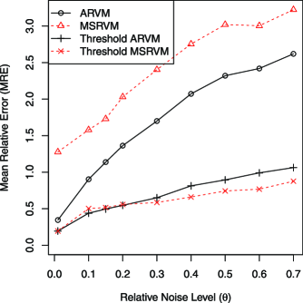
Figure 1: The MRE plots of the four estimators for $n=200$ and $p=100$.

Figure 1 is the plots of MRE versus relative noise level $\theta$ for the MSRVM, ARVM, threshold MSRVM and threshold ARVM estimators. The basic findings are that while the MREs of the threshold MSRVM and threshold ARVM estimators are comparable at low relative noise levels, the threshold MSRVM estimator has smaller MRE than the threshold ARVM estimator at high relative noise levels; regardless of relative noise levels, the threshold MSRVM and threshold ARVM estimators have significantly smaller MREs than the MSRVM and ARVM estimators. The simulation results support the theoretical conclusions that the threshold procedure is needed for constructing consistent estimators of $\bolds{\Gamma}$, and the threshold MSRVM estimator is asymptotically optimal, while the threshold ARVM estimator is suboptimal.

We point out that it is important to have a data-driven choice of tuning parameters for volatility matrix estimator defined in (7). This is largely an open issue. We briefly describe an approach for developing a data-dependent selection of the tuning parameters as follows. For data $\{Y_{i}(t_{\ell}),i=1,\ldots,p,\break\ell=1,\ldots,n\}$ observed from models (1)–(2), we may divide the whole data time interval into $L$ subintervals $I_{1},\ldots,I_{L}$, and partition data $Y_{i}(t_{\ell})$ into $L$ subsamples $\{Y_{i}(t_{\ell}),i=1,\ldots,p,t_{\ell}\in I_{k}\}$, $k=1,\ldots,L$, over the $L$ corresponding time periods. To estimate integrated volatility $\int_{I_{k}}\bolds{\gamma}(t)\,dt/|I_{k}|$ over the $k$th period, according to the procedure described in Section 2.2, we use the $k$th subsample to construct volatility matrix estimator, which is denoted by $\widehat{\Gamma}_{k}(N,\varpi)$ to emphasize its dependence on $N$ and $\varpi$, where $|I_{k}|$ denotes the length of $I_{k}$, $\varpi$ is a threshold value and $N$ is an integer that specifies scales used in the volatility matrix estimator given by (7). We predict one period ahead volatility matrix estimator $\widehat{\Gamma}_{k+1}(N,\varpi)$ by current period volatility matrix estimator $\widehat{\Gamma}_{k}(N,\varpi)$ and compute the predication error. We minimize the sum of the spectral norms of the predication errors to select $N$ and $\varpi$. For example, we often have high-frequency financial data over many days, and it is natural to use data in each day to estimate the integrated volatility matrix over the corresponding day. We predict one day ahead daily volatility matrix estimator by current daily volatility matrix estimator and compute the predication error. The tuning parameters are then selected by minimizing the sum of the spectral norms of the prediction errors.

6 Proofs

Denote by $C$’s generic constants whose values are free of $n$ and $p$ and may change from appearance to appearance. Let $u\vee v$ and $u\wedge v$ be the maximum and minimum of $u$ and $v$, respectively. For two sequences $u_{n,p}$ and $v_{n,p}$ we write $u_{n,p}\asymp v_{n,p}$ if there exist positive constants $C_{1}$ and $C_{2}$ free of $n$ and $p$ such that $C_{1}\leq u_{n,p}/v_{n,p}\leq C_{2}$. Without loss of generality we take $N=[n^{1/2}]$ in the construction of $\tilde{\bolds{\Gamma}}$ given by (5) in Section 2.2.

6.1 Proofs of Theorems 1 and 2

Let

$$\mathbf{Y}_{r}^{k_{m}} = \bigl{(}Y_{1}\bigl{(}\tau_{r}^{k_{m}}\bigr{)},\ldots,Y_{p}\bigl{(}\tau_{r}^{k_{m}}\bigr{)}\bigr{)}^{T},$$

$$\mathbf{X}_{r}^{k_{m}} = \bigl{(}X_{1}\bigl{(}\tau_{r}^{k_{m}}\bigr{)},\ldots,X_{p}\bigl{(}\tau_{r}^{k_{m}}\bigr{)}\bigr{)}^{T},$$

$$\bolds{\varepsilon}_{r}^{k_{m}} = \bigl{(}\varepsilon_{1}\bigl{(}\tau_{r}^{k_{m}}\bigr{)},\ldots,\varepsilon_{p}\bigl{(}\tau_{r}^{k_{m}}\bigr{)}\bigr{)}^{T},$$

which are random vectors corresponding to the data, the Itô process and the noises at the time point $\tau_{r}^{k_{m}}$, $r=1,\ldots,|\bolds{\tau}^{k_{m}}|$, $k_{m}=1,\ldots,K_{m}$, and $m=1,\ldots,N$. Note that we choose index $k_{m}$ to specify that the analyses are associated with the study of $\bolds{\Gamma}^{K_{m}}$ here and below. We decompose $\tilde{\bolds{\Gamma}}{}^{K_{m}}$ defined in (4) as follows:

$$\tilde{\bolds{\Gamma}}{}^{K_{m}} = \frac{1}{K_{m}}\sum_{k_{m}=1}^{K_{m}}\sum_{r=2}^{|\bolds{\tau}^{k_{m}}|}\bigl{(}\mathbf{Y}_{r}^{k_{m}}-\mathbf{Y}_{r-1}^{k_{m}}\bigr{)}\bigl{(}\mathbf{Y}_{r}^{k_{m}}-\mathbf{Y}_{r-1}^{k_{m}}\bigr{)}^{T}$$

$$= \frac{1}{K_{m}}\sum_{k_{m}=1}^{K_{m}}\sum_{r=2}^{|\bolds{\tau}^{k_{m}}|}\bigl{(}\mathbf{X}_{r}^{k_{m}}-\mathbf{X}_{r-1}^{k_{m}}+\bolds{\varepsilon}_{r}^{k_{m}}-\bolds{\varepsilon}_{r-1}^{k_{m}}\bigr{)}$$

$$\hskip 59.0pt{}\times\bigl{(}\mathbf{X}_{r}^{k_{m}}-\mathbf{X}_{r-1}^{k_{m}}+\bolds{\varepsilon}_{r}^{k_{m}}-\bolds{\varepsilon}_{r-1}^{k_{m}}\bigr{)}^{T}$$

$$= \frac{1}{K_{m}}\sum_{k_{m}=1}^{K_{m}}\sum_{r=2}^{|\bolds{\tau}^{k_{m}}|}\bigl{\{}\bigl{(}\mathbf{X}_{r}^{k_{m}}-\mathbf{X}_{r-1}^{k_{m}}\bigr{)}\bigl{(}\mathbf{X}_{r}^{k_{m}}-\mathbf{X}_{r-1}^{k_{m}}\bigr{)}^{T}$$

$$\hskip 66.0pt{}+\bigl{(}\bolds{\varepsilon}_{r}^{k_{m}}-\bolds{\varepsilon}_{r-1}^{k_{m}}\bigr{)}\bigl{(}\bolds{\varepsilon}_{r}^{k_{m}}-\bolds{\varepsilon}_{r-1}^{k_{m}}\bigr{)}^{T}$$

$$\hskip 66.0pt{}+\bigl{(}\mathbf{X}_{r}^{k_{m}}-\mathbf{X}_{r-1}^{k_{m}}\bigr{)}\bigl{(}\bolds{\varepsilon}_{r}^{k_{m}}-\bolds{\varepsilon}_{r-1}^{k_{m}}\bigr{)}^{T}$$

$$\hskip 66.0pt{}+\bigl{(}\bolds{\varepsilon}_{r}^{k_{m}}-\bolds{\varepsilon}_{r-1}^{k_{m}}\bigr{)}\bigl{(}\mathbf{X}_{r}^{k_{m}}-\mathbf{X}_{r-1}^{k_{m}}\bigr{)}^{T}\bigr{\}}$$

$$\equiv \mathbf{V}^{K_{m}}+\mathbf{G}^{K_{m}}(1)+\mathbf{G}^{K_{m}}(2)+\mathbf{G}^{K_{m}}(3),$$

and thus from (5) we obtain the corresponding decomposition for $\tilde{\bolds{\Gamma}}$,

$$\tilde{\bolds{\Gamma}} = \sum_{m=1}^{N}a_{m}\mathbf{V}^{K_{m}}+\zeta\bigl{(}\mathbf{V}^{K_{1}}-\mathbf{V}^{K_{N}}\bigr{)}$$

$${}+\sum_{r=1}^{3}\Biggl{[}\sum_{m=1}^{N}a_{m}\mathbf{G}^{K_{m}}(r)+\zeta\bigl{(}\mathbf{G}^{K_{1}}(r)-\mathbf{G}^{K_{N}}(r)\bigr{)}\Biggr{]}$$

$$\equiv \mathbf{V}+\mathbf{G}(1)+\mathbf{G}(2)+\mathbf{G}(3),$$

where the $\mathbf{V}^{k_{m}}$ and $\mathbf{V}$ terms are associated with the process $\mathbf{X}(t)$ only, the $\mathbf{G}^{K_{m}}(1)$ and $\mathbf{G}(1)$ terms are related to the noises $\varepsilon_{i}(t_{\ell})$ only and the terms denoted by $\mathbf{G}^{K_{m}}(2)$, $\mathbf{G}^{K_{m}}(3)$, $\mathbf{G}(2)$ and $\mathbf{G}(3)$ depend on both $\mathbf{X}(t)$ and $\varepsilon_{i}(t_{\ell})$.

Now we may heuristically explain the basic ideas for proving Theorems 1 and 2 as follows. With the expression (6.1) we prove the tail probability result for $\tilde{\bolds{\Gamma}}$ in Theorem 1 by establishing tail probabilities for these $\mathbf{V}$ and $\mathbf{G}$ terms in the following three propositions whose proofs will be given in Appendix I.

Proposition 5

Under the assumptions of Theorem 1, we have for $1\leq i,j\leq p$ and positive $d$ in a neighbor of $0$,

$$P\bigl{(}|V_{ij}-\Gamma_{ij}|\geq d\bigr{)}\leq C_{1}n\exp\bigl{\{}-\sqrt{n}d^{2}/C_{2}\bigr{\}}.$$

Proposition 6

Under the assumptions of Theorem 1, we have for $1\leq i,j\leq p$ and positive $d$ in a neighbor of $0$,

$$P\bigl{(}\bigl{|}G_{ij}(2)\bigr{|}\geq d\bigr{)} \leq C_{1}n\exp\bigl{\{}-\sqrt{n}d^{2}/C_{2}\bigr{\}},$$

$$P\bigl{(}\bigl{|}G_{ij}(3)\bigr{|}\geq d\bigr{)} \leq C_{1}n\exp\bigl{\{}-\sqrt{n}d^{2}/C_{2}\bigr{\}}.$$

Proposition 7

Under the assumptions of Theorem 1, we have for $1\leq i,j\leq p$ and positive $d$ in a neighbor of $0$,

$$P\bigl{(}\bigl{|}G_{ij}(1)\bigr{|}\geq d\bigr{)}\leq C_{1}\sqrt{n}\exp\bigl{\{}-\sqrt{n}d^{2}/C_{2}\bigr{\}}.$$

Because $V_{ij}$ are quadratic forms in the process $\mathbf{X}(t_{\ell})$ only, we derive their tail probability in Proposition 5 from the boundedness of the drift and volatility in condition A2; as $G_{ij}(1)$ are quadratic forms in the noises $\varepsilon_{i}(t_{\ell})$ only, we establish the tail probability of $G_{ij}(1)$ in Proposition 7 from the subGaussianity of $\varepsilon_{i}(t_{\ell})$ imposed by condition A1; $G_{ij}(2)$ and $G_{ij}(3)$ are bilinear forms in $\mathbf{X}(t_{\ell})$ and $\varepsilon_{i}(t_{\ell})$, thus we obtain the tail probabilities for $G_{ij}(2)$ and $G_{ij}(3)$ in Proposition 6 from the subGaussian tails of $\varepsilon_{i}(t_{\ell})$ and $V_{ij}$ as well as the independence between $\varepsilon_{i}(t_{\ell})$ and $\mathbf{X}(t)$ given by condition A1. Since $\widehat{\bolds{\Gamma}}$ is the matrix estimator obtained by thresholding $\tilde{\bolds{\Gamma}}$, we use the tail probability result in Theorem 1 and the sparsity of $\bolds{\Gamma}$ to analyze $\widehat{\bolds{\Gamma}}-\bolds{\Gamma}$ and control its matrix norm for proving Theorem 2.

Proof of Theorem 1 From (6.1) we have

$$P\bigl{(}|\tilde{\Gamma}_{ij}-\Gamma_{ij}|\geq x\bigr{)}\leq P\bigl{(}|V_{ij}-\Gamma_{ij}|\geq x/4\bigr{)}+\sum_{r=1}^{3}P\bigl{(}\bigl{|}G_{ij}(r)\bigr{|}\geq x/4\bigr{)},$$

and thus the theorem is a consequence of Propositions 5–7.

Proof of Theorem 2 Define

$$A_{ij} = \bigl{\{}|\widehat{\Gamma}_{ij}-\Gamma_{ij}|\leq 2\min\bigl{\{}|\Gamma_{ij}|,\varpi\bigr{\}}\bigr{\}},\qquad D_{ij}=(\widehat{\Gamma}_{ij}-\Gamma_{ij})1\bigl{(}A_{ij}^{c}\bigr{)},$$

$$\mathbf{D} = (D_{ij})_{1\leq i,j\leq p}.$$

As the matrix norm of a symmetric matrix is bounded by its $\ell_{1}$-norm, then

$$E\|\widehat{\bolds}{\Gamma}-\bolds{\Gamma}\|_{2}^{2}\leq E\|\widehat{\bolds}{\Gamma}-\bolds{\Gamma}\|_{1}^{2}\leq 2E\|\widehat{\bolds}{\Gamma}-\bolds{\Gamma}-\mathbf{D}\|_{1}^{2}+2E\|\mathbf{D}\|_{1}^{2}.$$ (27)

We can bound $E\|\widehat{\bolds}{\Gamma}-\bolds{\Gamma}-\mathbf{D}\|^{2}_{1}$ as follows:

$$E\|\widehat{\bolds}{\Gamma}-\bolds{\Gamma}-\mathbf{D}\|_{1}^{2}$$

$$\qquad=E\Biggl{[}\max_{1\leq j\leq p}\sum_{i=1}^{p}|\widehat{\Gamma}_{ij}-\Gamma_{ij}|1\bigl{(}|\widehat{\Gamma}_{ij}-\Gamma_{ij}|\leq 2\min\bigl{\{}|\Gamma_{ij}|,\varpi\bigr{\}}\bigr{)}\Biggr{]}^{2}$$

$$\qquad\leq E\Biggl{[}\max_{1\leq j\leq p}\sum_{i=1}^{p}2|\Gamma_{ij}|1\bigl{(}|\Gamma_{ij}|<\varpi\bigr{)}\Biggr{]}^{2}$$

$$\qquad\quad{}+E\Biggl{[}\max_{1\leq j\leq p}\sum_{i=1}^{p}2\varpi 1\bigl{(}|\Gamma_{ij}|\geq\varpi\bigr{)}\Biggr{]}^{2}$$

$$\qquad\leq 8E\bigl{[}\Psi^{2}\bigr{]}\pi_{n}^{2}(p)\varpi^{2(1-q)}\leq C\pi_{n}^{2}(p)\bigl{(}n^{-1/4}\sqrt{\log p}\bigr{)}^{2-2q},$$

where the second inequality is due to the fact that the sparsity of $\bolds{\Gamma}$ implies

$$\max_{1\leq j\leq p}\sum_{i=1}^{p}1\bigl{(}|\Gamma_{ij}|\geq\varpi\bigr{)} \leq \Psi\pi_{n}(p)\varpi^{-q},$$

$$\max_{1\leq j\leq p}\sum_{i=1}^{p}|\Gamma_{ij}|1\bigl{(}|\Gamma_{ij}|<\varpi\bigr{)} \leq \Psi\pi_{n}(p)\varpi^{1-q},$$

which are the respective bounds on the number of those entries on each row with absolute values larger than or equal to $\varpi$ and the sum of those absolute entries on each row with magnitudes less than $\varpi$; see Lemma 1 in Wang and Zou (2010). The rest of the proof is to show that $E\|\mathbf{D}\|_{1}^{2}=O(n^{-2})$, a negligible term. Indeed, the threshold rule indicates that $\widehat{\Gamma}_{ij}=0$ if $|\tilde{\Gamma}_{ij}|<\varpi$ and $\widehat{\Gamma}_{ij}=\tilde{\Gamma}_{ij}$ if $|\tilde{\Gamma}_{ij}|\geq\varpi$, thus

$$E\|\mathbf{D}\|_{1}^{2} \leq p\sum_{i,j=1}^{p}E\bigl{[}|\Gamma_{ij}|^{2}1\bigl{(}|\Gamma_{ij}|>2\min\bigl{\{}|\Gamma_{ij}|,\varpi\bigr{\}}\bigr{)}1(\widehat{\Gamma}_{ij}=0)\bigr{]}$$

$${}+p\sum_{i,j}^{p}E\bigl{[}|\tilde{\Gamma}_{ij}-\Gamma_{ij}|^{2}1\bigl{(}|\tilde{\Gamma}_{ij}-\Gamma_{ij}|>2\min\bigl{\{}|\Gamma_{ij}|,\varpi\bigr{\}}\bigr{)}1(\widehat{\Gamma}_{ij}=\tilde{\Gamma}_{ij})\bigr{]}$$

$$\equiv I_{1}+I_{2}.$$

For term $I_{1}$, we have

$$I_{1} \leq p\sum_{i,j=1}^{p}E\bigl{[}|\Gamma_{ij}|^{2}1\bigl{(}|\tilde{\Gamma}_{ij}-\Gamma_{ij}|>\varpi\bigr{)}\bigr{]}\leq Cp\sum_{i,j=1}^{p}P\bigl{(}|\tilde{\Gamma}_{ij}-\Gamma_{ij}|>\varpi\bigr{)}$$

$$\leq Cp^{3}\exp\bigl{\{}\log n-\sqrt{n}\varpi^{2}/\varsigma_{0}\bigr{\}}\leq Cn^{-2},$$

where the third inequality is from Theorem 1, and the last inequality is due to $\varpi=\hbar n^{-1/4}\sqrt{\log(np)}$ with $\hbar^{2}/\varsigma_{0}>4$.

On the other hand, we can bound term $I_{2}$ as follows:

$$I_{2} \leq p\sum_{i,j=1}^{p}E\bigl{[}|\tilde{\Gamma}_{ij}-\Gamma_{ij}|^{2}1\bigl{(}|\tilde{\Gamma}_{ij}-\Gamma_{ij}|>\varpi\bigr{)}\bigr{]}$$

$${}+p\sum_{i,j=1}^{p}E\bigl{[}|\tilde{\Gamma}_{ij}-\Gamma_{ij}|^{2}1\bigl{(}|\Gamma_{ij}|<\varpi/2,|\tilde{\Gamma}_{ij}|\geq\varpi\bigr{)}\bigr{]}$$

$$\leq 2p\sum_{i,j=1}^{p}E\bigl{[}|\tilde{\Gamma}_{ij}-\Gamma_{ij}|^{2}1\bigl{(}|\tilde{\Gamma}_{ij}-\Gamma_{ij}|>\varpi/2\bigr{)}\bigr{]}$$

$$\leq 2p\sum_{i,j=1}^{p}\bigl{\{}E\bigl{[}|\tilde{\Gamma}_{ij}-\Gamma_{ij}|^{4}\bigr{]}P\bigl{(}|\tilde{\Gamma}_{ij}-\Gamma_{ij}|>\varpi/2\bigr{)}\bigr{\}}^{1/2}$$

$$\leq Cp^{3}\exp\bigl{\{}\log n/2-\sqrt{n}\varpi^{2}/(8\varsigma_{0})\bigr{\}}\leq Cn^{-2},$$

where the third inequality is due to Hölder’s inequality, the fourth inequality is from Theorem 1 and

$$\max_{1\leq i,j\leq p}E\bigl{[}|\tilde{\Gamma}_{ij}-\Gamma_{ij}|^{4}\bigr{]}\leq C$$ (28)

and the last inequality is due to the fact that $\varpi=\hbar n^{-1/4}\sqrt{\log(np)}$ with $\hbar^{2}/(8\varsigma_{0})>3$.

To complete the proof we need to show (28). As in Zhang, Mykland and Aït-Sahalia (2005), we adjust $\tilde{\bolds{\Gamma}}{}^{K_{m}}$ to account for the noise variances. Let

$$\tilde{\bolds{\eta}}=\operatorname{diag}(\tilde{\eta}_{1},\ldots,\tilde{\eta}_{p}),\qquad\tilde{\eta}_{i}=\frac{1}{2n}\sum_{\ell=2}^{n}\bigl{[}Y_{i}(t_{\ell})-Y_{i}(t_{\ell-1})\bigr{]}^{2},$$ (29)

and define

$$\tilde{\bolds{\Gamma}}{}^{*K_{m}}=\tilde{\bolds{\Gamma}}{}^{K_{m}}-2\frac{n-K_{m}+1}{K_{m}}\tilde{\bolds{\eta}},$$ (30)

which are the average realized volatility matrix (ARVM) estimators where the convergence rates for any finite moments of $\tilde{\Gamma}{}^{*K_{m}}_{ij}-\Gamma_{ij}$ are derived in Wang and Zou [(2010), Theorem 1]. Applying Theorem 1 of Wang and Zou (2010) to the fourth moment of $\tilde{\Gamma}{}^{*K_{m}}_{ij}-\Gamma_{ij}$, we have for $1\leq i,j\leq p$ and $1\leq m\leq N$,

$$E\bigl{(}\bigl{|}\tilde{\Gamma}{}^{*K_{m}}_{ij}-\Gamma_{ij}\bigr{|}^{4}\bigr{)}$$

(31)

$$\qquad\leq C\bigl{[}\bigl{(}K_{m}n^{-1/2}\bigr{)}^{-4}+K_{m}^{-2}+(n/K_{m})^{-2}+K_{m}^{-4}+n^{-2}\bigr{]}\leq C.$$

From (5), (6) and (30) together with simple algebraic manipulations we can express $\tilde{\bolds{\Gamma}}$ by $\tilde{\bolds{\Gamma}}{}^{*K_{m}}$ as follows:

$$\tilde{\bolds{\Gamma}}=\sum_{m=1}^{N}a_{m}\tilde{\bolds{\Gamma}}{}^{*K_{m}}+\zeta\bigl{(}\tilde{\bolds{\Gamma}}{}^{*K_{1}}-\tilde{\bolds{\Gamma}}{}^{*K_{N}}\bigr{)},$$

and thus

$$\tilde{\bolds{\Gamma}}-\bolds{\Gamma}=\sum_{m=1}^{N}a_{m}\bigl{(}\tilde{\bolds{\Gamma}}{}^{*K_{m}}-\bolds{\Gamma}\bigr{)}+\zeta\bigl{[}\bigl{(}\tilde{\bolds{\Gamma}}{}^{*K_{1}}-\bolds{\Gamma}\bigr{)}-\bigl{(}\tilde{\bolds{\Gamma}}{}^{*K_{N}}-\bolds{\Gamma}\bigr{)}\bigr{]}.$$ (32)

Combining (6.1) and (32) and using (6) we conclude for $1\leq i,j\leq p$,

$$E\bigl{[}|\tilde{\Gamma}_{ij}-\Gamma_{ij}|^{4}\bigr{]}$$

$$\qquad\leq(N+2)^{3}\Biggl{[}\sum_{m=1}^{N}a_{m}^{4}E\bigl{(}\bigl{|}\tilde{\Gamma}{}^{*K_{m}}_{ij}-\Gamma_{ij}\bigr{|}^{4}\bigr{)}$$

$$\hskip 75.0pt\qquad{}+\zeta^{4}E\bigl{(}\bigl{|}\tilde{\bolds{\Gamma}}{}^{*K_{1}}-\Gamma_{ij}\bigr{|}^{4}+\bigl{|}\tilde{\bolds{\Gamma}}{}^{*K_{N}}-\Gamma_{ij}\bigr{|}^{4}\bigr{)}\Biggr{]}$$

$$\qquad\leq C.$$

6.2 Proofs of Theorems 3 and 4

Section 4.1 shows that Theorem 3 is a consequence of Theorem 4. The proof of Theorem 4 is similar to but much more involved than the proof of Theorem 2 in Cai and Zhou (2012) which considered only i.i.d. observations. It contains four major steps. In the first step we construct in detail a finite subset $\mathcal{F}_{\ast}$ of the parameter space $\mathcal{G}_{q}(\pi_{n}(p))$ in the minimax problem $\mathcal{Q}_{q}(\pi_{n}(p))$ such that the difficulty of estimation over $\mathcal{F}_{\ast}$ is essentially the same as that of estimation over $\mathcal{G}_{q}(\pi_{n}(p))$, where $\mathcal{G}_{q}(\pi_{n}(p))$ is the class of constant matrices $\bolds{\Gamma}$ satisfying (18) and $\|\bolds{\Gamma}\|_{2}\leq\tau$ for constant $\tau>0$. The second step applies the lower bound argument in Cai and Zhou [(2012), Lemma 3] to the carefully constructed parameter set $\mathcal{F}_{\ast}$. In the third step we calculate the factor $\alpha$ defined in (6.2) below and the total variation affinity between two average of products of $n$ independent but nonidentically distributed multivariate normals. The final step combines together the results in steps 2 and 3 to obtain the minimax lower bound.

Step 1: Construct parameter set ${\mathcal{F}}_{*}$. Set $r=\lceil p/2\rceil$, where $\lceil x\rceil$ denotes the smallest integer greater than or equal to $x$, and let $B$ be the collection of all row vectors $b=(v_{j})_{1\leq j\leq p}$ such that $v_{j}=0$ for $1\leq j\leq p-r$ and $v_{j}=0$ or $1$ for $p-r+1\leq j\leq p$ under the constraint $\|b\|_{0}=k$ (to be specified later). Each element $\lambda=(b_{1},\ldots,b_{r})\in B^{r}$ is treated as an $r\times p$ matrix with the $i$th row of $\lambda$ equal to $b_{i}$. Let $\Delta=\{0,1\}^{r}$. Define $\Lambda\subset B^{r}$ to be the set of all elements in $B^{r}$ such that each column sum is less than or equal to $2k$. For each $b\in B$ and each $1\leq m\leq r$, define a $p\times p$ symmetric matrix $A_{m}(b)$ by making the $m$th row of $A_{m}(b)$ equal to $b$, $m$th column equal to $b^{T}$ and the rest of the entries $0$. Then each component $\lambda_{i}$ of $\lambda=(\lambda_{1},\ldots,\lambda_{r})\in\Lambda$ can be uniquely associated with a $p\times p$ matrix $A_{i}(\lambda_{i})$. Define $\Theta=\Delta\otimes\Lambda$, and let $\epsilon_{n,p}\in\mathbb{R}$ be fixed (the exact value of $\epsilon_{n,p}$ will be chosen later). For each $\theta=(\gamma,\lambda)\in\Theta$ with $\gamma=(\gamma_{1},\ldots,\gamma_{r})\in\Delta$ and $\lambda=(\lambda_{1},\ldots,\lambda_{r})\in\Lambda$, we associate $\theta=(\gamma_{1},\ldots,\gamma_{r},\lambda_{1},\ldots,\lambda_{r})$ with a volatility matrix $\bolds{\Gamma}(\theta)$ by

$$\bolds{\Gamma}(\theta)=\mathbf{I}_{p}+\epsilon_{n,p}\sum_{m=1}^{r}\gamma_{m}A_{m}(\lambda_{m}).$$ (33)

For simplicity we assume that $\tau>1$ in the definition of the parameter space $\mathcal{G}_{q}(\pi_{n}(p))$ for the minimax problem $\mathcal{Q}_{q}(\pi_{n}(p))$; otherwise we replace $\mathbf{I}_{p}$ in (33) by $C\mathbf{I}_{p}$ with a small constant $C>0$. Finally we define $\mathcal{F}_{\ast}$ to be a collection of covariance matrices as

$$\mathcal{F}_{\ast}=\Biggl{\{}\bolds{\Gamma}(\theta)\dvtx\bolds{\Gamma}(\theta)=\mathbf{I}_{p}+\epsilon_{n,p}\sum_{m=1}^{r}\gamma_{m}A_{m}(\lambda_{m}),\theta=(\gamma,\lambda)\in\Theta\Biggr{\}}.$$ (34)

Note that each matrix $\bolds{\Gamma}\in\mathcal{F}_{\ast}$ has value $1$ along the main diagonal and contains an $r\times r$ submatrix, say, $A$, at the upper right corner, $A^{T}$ at the lower left corner and $0$ elsewhere; each row of the submatrix $A$ is either identically $0$ (if the corresponding $\gamma$ value is $0$) or has exactly $k$ nonzero elements with value $\epsilon_{n,p}$.

Now we specify the values of $\epsilon_{n,p}$ and $k$:

$$\epsilon_{n,p}=\upsilon\biggl{(}\frac{\log p}{\sqrt{n}}\biggr{)}^{1/2},\qquad k=\biggl{\lceil}\frac{1}{2}\pi_{n}(p)\epsilon_{n,p}^{-q}\biggr{\rceil}-1,$$ (35)

where $\upsilon$ is a fixed small constant that we require

$$0<\upsilon<\biggl{[}\min\biggl{\{}\frac{1}{3},\tau-1\biggr{\}}\frac{1}{\aleph}\biggr{]}^{{1}/{(1-q)}}$$ (36)

and

$$0<\upsilon^{2}<\frac{\beta-1}{27c_{\kappa}\beta},$$ (37)

where $c_{\kappa}=(2\kappa)^{-1}$ satisfies

$$\sum_{l=1}^{n}a_{l}^{-2}\leq c_{\kappa}\sqrt{n},$$ (38)

since

$$\sum_{l=1}^{n}a_{l}^{-2} \leq \int_{0}^{n}\biggl{[}1+4\kappa^{2}n\sin^{2}\biggl{(}\frac{\pi x}{2(n+1)}\biggr{)}\biggr{]}^{-2}\,dx\leq\frac{n+1}{\pi\kappa\sqrt{n}}\int_{0}^{\infty}\bigl{[}1+v^{2}\bigr{]}^{-2}\,dv$$

$$= \frac{\sqrt{n}+1/\sqrt{n}}{4\kappa}.$$

Note that $\epsilon_{n,p}$ and $k$ satisfy $\max_{j\leq p}\sum_{i\neq j}|\Gamma_{ij}|^{q}\leq 2k\epsilon_{n,p}^{q}\leq\pi_{n}(p)$,

$$2k\epsilon_{n,p}\leq\pi_{n}(p)\epsilon_{n,p}^{1-q}\leq\aleph\upsilon^{1-q}<\min\bigl{\{}\tfrac{1}{3},\tau-1\bigr{\}},$$ (39)

and consequently every $\bolds{\Gamma}(\theta)$ is diagonally dominant and positive definite, and $\|\bolds{\Gamma}(\theta)\|_{2}\leq\|\bolds{\Gamma}(\theta)\|_{1}\leq 2k\epsilon_{n,p}+1<\tau$. Thus we have $\mathcal{F}_{\ast}\subset\mathcal{G}_{q}(\pi_{n}(p))$.

Step 2: Apply the general lower bound argument. Let $\mathbf{U}_{l}$ be independent with

$$\mathbf{U}_{l}\sim N\bigl{(}0,\bolds{\Gamma}(\theta)+(a_{l}-1)\mathbf{I}_{p}\bigr{)},$$

where $l=1,\ldots,n$, $\theta\in\Theta$, and we denote the joint distribution by $P_{\theta}$. Applying Lemma 3 in Cai and Zhou (2012) to the parameter space $\Theta$, we have

$$\inf_{\check{\bolds{\Gamma}}}\max_{\theta\in\Theta}\mathbb{E}_{\theta}\bigl{\|}\check{\bolds{\Gamma}}-\bolds{\Gamma}(\theta)\bigr{\|}_{2}^{2}\geq\alpha\cdot\frac{r}{8}\cdot\min_{1\leq i\leq r}\|\bar{\mathbb{P}}_{i,0}\wedge\bar{\mathbb{P}}_{i,1}\|,$$ (40)

where we use $\|\mathbb{P}\|$ to denote the total variation of $\mathbb{P}$,

$$\alpha \equiv \min_{\{(\theta,\theta^{\prime})\dvtx H(\gamma(\theta),\gamma(\theta^{\prime}))\geq 1\}}\frac{\|\bolds{\Gamma}(\theta)-\bolds{\Gamma}(\theta^{\prime})\|_{2}^{2}}{H(\gamma(\theta),\gamma(\theta^{\prime}))},$$

$$H\bigl{(}\gamma(\theta),\gamma\bigl{(}\theta^{\prime}\bigr{)}\bigr{)} = \sum_{i=1}^{r}\bigl{|}\gamma_{i}(\theta)-\gamma_{i}\bigl{(}\theta^{\prime}\bigr{)}\bigr{|}$$

and

$$\bar{\mathbb{P}}_{i,a}=\frac{1}{2^{r-1}D_{\Lambda}}\sum_{\theta\in\Theta}\mathbb{P}_{\theta}\cdot\bigl{\{}\theta\dvtx\gamma_{i}(\theta)=a\bigr{\}},$$ (42)

where $a\in\{0,1\}$ and $D_{\Lambda}=\mathrm{Card}\{\Lambda\}$.

Step 3: Bound the affinity and per comparison loss. We need to bound the two factors $\alpha$ and $\min_{i}\|\bar{\mathbb{P}}_{i,0}\wedge\bar{\mathbb{P}}_{i,1}\|$ in (40). A lower bound for $\alpha$ is given by the following proposition whose proof is the same as that of Lemma 5 in Cai and Zhou (2012).

Proposition 8

For $\alpha$ defined in equation (6.2) we have

$$\alpha\geq\frac{(k\epsilon_{n,p})^{2}}{p}.$$

A lower bound for $\min_{i}\|\bar{\mathbb{P}}_{i,0}\wedge\bar{\mathbb{P}}_{i,1}\|$ is provided by the proposition below. Since its proof is long and very much involved, the proof details are collected in Appendix II.

Proposition 9

Let $\mathbf{U}_{l}$ be independent with $\mathbf{U}_{l}\sim N(0,\bolds{\Gamma}(\theta)+(a_{l}-1)\mathbf{I}_{p})$, $l=1,\ldots,n$, with $\theta\in\Theta$ and denote the joint distribution by $\mathbb{P}_{\theta}$. For $a\in\{0,1\}$ and $1\leq i\leq r$, define $\bar{\mathbb{P}}_{i,a}$ as in (42). Then there exists a constant $C_{1}>0$ such that

$$\min_{1\leq i\leq r}\|\bar{\mathbb{P}}_{i,0}\wedge\bar{\mathbb{P}}_{i,1}\|\geq C_{1}$$

uniformly over $\Theta$.

Step 4: Obtain the minimax lower bound. We obtain the minimax lower bound for estimating $\bolds{\Gamma}$ over $\mathcal{G}_{q}(\pi_{n}(p))$ by combining together (40) and the bounds in Propositions 8 and 9,

$$\inf_{\check{\bolds{\Gamma}}}\sup_{\mathcal{G}_{q}(\pi_{n}(p))}\mathbb{E}\|\check{\bolds{\Gamma}}-\bolds{\Gamma}\|_{2}^{2} \geq \inf_{\check{\bolds{\Gamma}}}\max_{\bolds{\Gamma}(\theta)\in\mathcal{F}_{\ast}}\mathbb{E}_{\theta}\bigl{\|}\check{\bolds{\Gamma}}-\bolds{\Gamma}(\theta)\bigr{\|}_{2}^{2}\geq\frac{(k\epsilon_{n,p})^{2}}{p}\cdot\frac{r}{8}\cdot C_{1}$$

$$\geq \frac{C_{1}}{16}(k\epsilon_{n,p})^{2}=C_{2}\pi^{2}_{n}(p)\bigl{(}n^{-1/4}\sqrt{\log p}\bigr{)}^{2-2q}$$

for some constant $C_{2}>0$.

6.3 Proof of (3) for optimal convergence rate under general matrix norm

The Riesz–Thorin interpolation theorem [Thorin (1948)] implies for $1\leq d_{1}\leq d\leq d_{2}\leq\infty$,

$$\|\mathbf{A}\|_{d}\leq\max\bigl{\{}\|\mathbf{A}\|_{d_{1}},\|\mathbf{A}\|_{d_{2}}\bigr{\}}.$$ (43)

Set $d_{1}=1$ and $d_{2}=\infty$, then (43 ) yields $\|\mathbf{A}\|_{d}\leq\max\{\|\mathbf{A}\|_{1},\|\mathbf{A}\|_{\infty}\}$ for $1\leq d\leq\infty$. When $\mathbf{A}$ is symmetric, (8) shows that $\|\mathbf{A}\|_{1}=\|\mathbf{A}\|_{\infty}$. Then immediately we have $\|\mathbf{A}\|_{d}\leq\|\mathbf{A}\|_{1}$, which means that for a symmetric matrix estimator, an upper bound under the matrix $\ell_{1}$ norm is also an upper bound under the general matrix $\ell_{d}$ norm. Thus, as $\widehat{\bolds}{\Gamma}$ is symmetric, Theorem 2 indicates that for $1\leq d\leq\infty$,

$$\sup_{\mathcal{P}_{q}(\pi_{n}(p))}\mathbb{E}\|\widehat{\bolds}{\Gamma}-\bolds{\Gamma}\|_{d}^{2}\leq C^{*}\bigl{[}\pi_{n}(p)\bigl{(}n^{-1/4}\sqrt{\log p}\bigr{)}^{1-q}\bigr{]}^{2}.$$

Now consider the lower bound under the general matrix $\ell_{d}$ norm for $1\leq d\leq\infty$. We will show

$$\inf_{\check{\bolds{\Gamma}}_{s}}\sup_{\mathcal{P}_{q}(\pi_{n}(p))}\mathbb{E}\|\check{\bolds{\Gamma}}_{s}-\bolds{\Gamma}\|_{d}^{2} \geq \inf_{\check{\bolds{\Gamma}}}\sup_{\mathcal{P}_{q}(\pi_{n}(p))}\mathbb{E}\|\check{\bolds{\Gamma}}-\bolds{\Gamma}\|_{d}^{2}$$

$$\geq \frac{1}{4}\inf_{\check{\bolds{\Gamma}}_{s}}\sup_{\mathcal{P}_{q}(\pi_{n}(p))}\mathbb{E}\|\check{\bolds{\Gamma}}_{s}-\bolds{\Gamma}\|_{d}^{2},$$

where $\check{\bolds{\Gamma}}$ denotes any matrix estimators of $\bolds{\Gamma}$, and $\check{\bolds{\Gamma}}_{s}$ any symmetric matrix estimators of $\bolds{\Gamma}$. (6.3) indicates that it is enough to consider estimators of symmetric matrices.

For symmetric $\mathbf{A}$, (9) shows that $\|\mathbf{A}\|_{2}\leq\|\mathbf{A}\|_{1}=\|\mathbf{A}\|_{\infty}$. For $d\in(1,\infty)$, $1/d+(d-1)/d=1$, by duality we have $\|\mathbf{A}\|_{d}=\|\mathbf{A}\|_{{d}/{(d-1)}}$. Also since $2$ is always between $d$ and $d/(d-1)$, applying (43) we obtain that $\|\mathbf{A}\|_{2}\leq\max\{\|\mathbf{A}\|_{d},\|\mathbf{A}\|_{{d}/{(d-1)}}\}=\|\mathbf{A}\|_{d}$. This means that within the class of symmetric matrix estimators, a lower bound under the matrix $\ell_{2}$ norm is also a lower bound under the general matrix $\ell_{d}$ norm. Thus (6.3) and Theorem 3 together imply that for $1\leq d\leq\infty$,

$$\inf_{\check{\bolds{\Gamma}}}\sup_{\mathcal{P}_{q}(\pi_{n}(p))}\mathbb{E}\|\check{\bolds{\Gamma}}-\bolds{\Gamma}\|_{d}^{2}\geq\frac{C_{*}}{4}\bigl{[}\pi_{n}(p)\bigl{(}n^{-1/4}\sqrt{\log p}\bigr{)}^{1-q}\bigr{]}^{2}.$$

To complete the proof we need to prove (6.3). The first inequality of (6.3) is obvious. For a given matrix estimator $\check{\bolds{\Gamma}}$ we project it onto the parameter space of the minimax problem $\mathcal{P}_{q}(\pi_{n}(p))$ by minimizing the matrix $\ell_{d}$ norm of $\check{\bolds{\Gamma}}-\bolds{\Gamma}_{*}$ over all $\bolds{\Gamma}_{*}$ in the parameter space. Denote its projection by $\check{\bolds{\Gamma}}_{p}$. Since the parameter space consists of symmetric matrices, $\check{\bolds{\Gamma}}_{p}$ is symmetric. Hence

$$\inf_{\check{\bolds{\Gamma}}_{s}}\sup_{\mathcal{P}_{q}(\pi_{n}(p))}\mathbb{E}\|\check{\bolds{\Gamma}}_{s}-\bolds{\Gamma}\|_{d}^{2}$$

$$\qquad\leq\sup_{\mathcal{P}_{q}(\pi_{n}(p))}\mathbb{E}\|\check{\bolds{\Gamma}}_{p}-\bolds{\Gamma}\|_{d}^{2}$$

$$\qquad\leq 2\sup_{\mathcal{P}_{q}(\pi_{n}(p))}\bigl{[}\mathbb{E}\|\check{\bolds{\Gamma}}_{p}-\check{\bolds{\Gamma}}\|_{d}^{2}+\mathbb{E}\|\check{\bolds{\Gamma}}-\bolds{\Gamma}\|_{d}^{2}\bigr{]}$$

$$\qquad\leq 2\sup_{\mathcal{P}_{q}(\pi_{n}(p))}\bigl{[}\mathbb{E}\|\bolds{\Gamma}-\check{\bolds{\Gamma}}\|_{d}^{2}+\mathbb{E}\|\check{\bolds{\Gamma}}-\bolds{\Gamma}\|_{d}^{2}\bigr{]}$$

$$\qquad\leq 4\sup_{\mathcal{P}_{q}(\pi_{n}(p))}\mathbb{E}\|\check{\bolds{\Gamma}}-\bolds{\Gamma}\|_{d}^{2},$$

where the second inequality is from the triangle inequality and the third one follows from the definition of $\check{\bolds{\Gamma}}_{p}$. Since the above inequality holds for every $\check{\bolds{\Gamma}}$, we have

$$\inf_{\check{\bolds{\Gamma}}_{s}}\sup_{\mathcal{P}_{q}(\pi_{n}(p))}\mathbb{E}\|\check{\bolds{\Gamma}}_{s}-\bolds{\Gamma}\|_{d}^{2}$$

$$\qquad\leq 4\inf_{\check{\bolds{\Gamma}}}\sup_{\mathcal{P}_{q}(\pi_{n}(p))}\mathbb{E}\|\check{\bolds{\Gamma}}-\bolds{\Gamma}\|_{d}^{2},$$

which is equivalent to the second inequality of (6.3).

Appendix I Proofs of Propositions 5–7

I.1 Proof of Proposition 5

From the expression of $V_{ij}$ in terms of $V^{K_{m}}_{ij}$ given by (6.1), we have

$$P\bigl{(}|V_{ij}-\Gamma_{ij}|\geq d\bigr{)}$$

$$\qquad\leq P\Biggl{(}\sum_{m=1}^{N}|a_{m}|\bigl{|}V^{K_{m}}_{ij}-\Gamma_{ij}\bigr{|}+\zeta\bigl{(}\bigl{|}V^{K_{1}}_{ij}-\Gamma_{ij}\bigr{|}+\bigl{|}V^{K_{N}}_{ij}-\Gamma_{ij}\bigr{|}\bigr{)}\geq d\Biggr{)}$$

$$\qquad\leq P\Biggl{(}\sum_{m=1}^{N}|a_{m}|\bigl{|}V^{K_{m}}_{ij}-\Gamma_{ij}\bigr{|}\geq d/2\Biggr{)}$$

(45)

$$\qquad\quad{}+P\bigl{(}\zeta\bigl{|}V^{K_{1}}_{ij}-\Gamma_{ij}\bigr{|}+\zeta\bigl{|}V^{K_{N}}_{ij}-\Gamma_{ij}\bigr{|}\geq d/2\bigr{)}$$

$$\qquad\leq\sum_{m=1}^{N}P\bigl{(}\bigl{|}V^{K_{m}}_{ij}-\Gamma_{ij}\bigr{|}\geq d/(2A)\bigr{)}+P\bigl{(}\zeta\bigl{|}V^{K_{1}}_{ij}-\Gamma_{ij}\bigr{|}\geq d/4\bigr{)}$$

$$\qquad\quad{}+P\bigl{(}\zeta\bigl{|}V^{K_{N}}_{ij}-\Gamma_{ij}\bigr{|}\geq d/4\bigr{)},$$

where $A=\sum_{m=1}^{N}|a_{m}|=9/2+o(1)$.

The definition of $V_{ij}^{K_{m}}$ in (6.1) shows

$$V_{ij}^{K_{m}} = \frac{1}{K_{m}}\sum_{k_{m}=1}^{K_{m}}\sum_{r=2}^{|\bolds{\tau}^{k_{m}}|}\bigl{\{}X_{i}\bigl{(}\tau_{r}^{k_{m}}\bigr{)}-X_{i}\bigl{(}\tau_{r-1}^{k_{m}}\bigr{)}\bigr{\}}\bigl{\{}X_{j}\bigl{(}\tau_{r}^{k_{m}}\bigr{)}-X_{j}\bigl{(}\tau_{r-1}^{k_{m}}\bigr{)}\bigr{\}}$$

$$\equiv \frac{1}{K_{m}}\sum_{k_{m}=1}^{K_{m}}[X_{i},X_{j}]^{(k_{m})}$$

and

$$V_{ij}^{K_{m}}-\Gamma_{ij}=\frac{1}{K_{m}}\sum_{k_{m}=1}^{K_{m}}\biggl{[}[X_{i},X_{j}]^{(k_{m})}-\int_{0}^{1}\gamma_{ij}(s)\,ds\biggr{]}.$$

With the above expression for $V^{K_{m}}_{ij}-\Gamma_{ij}$ we obtain that for $d_{1}>0$ and $1\leq m\leq N$,

$$P\bigl{(}\bigl{|}V^{K_{m}}_{ij}-\Gamma_{ij}\bigr{|}\geq d_{1}\bigr{)} \leq P\Biggl{(}\frac{1}{K_{m}}\sum_{k_{m}=1}^{K_{m}}\biggl{|}[X_{i},X_{j}]^{(k_{m})}-\int_{0}^{1}\gamma_{ij}(s)\,ds\biggr{|}\geq d_{1}\Biggr{)}$$

$$\leq \sum_{k_{m}=1}^{K_{m}}P\biggl{(}\biggl{|}[X_{i},X_{j}]^{(k_{m})}-\int_{0}^{1}\gamma_{ij}(s)\,ds\biggr{|}\geq d_{1}\biggr{)}$$

$$\leq C_{1}K_{m}\exp\biggl{\{}-\frac{n}{K_{m}}\frac{d_{1}^{2}}{C_{2}}\biggr{\}}\leq C_{3}\sqrt{n}\exp\bigl{\{}-\sqrt{n}d_{1}^{2}/C_{4}\bigr{\}},$$

where the third inequality is from Lemma 10 below and the last inequality is due to the fact that $\sqrt{n}\leq K_{m}\leq 2\sqrt{n}$ and the maximum distance between consecutive grids in $\tau^{k_{m}}$ is bounded by $K_{m}/n\leq 2/\sqrt{n}$.

Substituting (I.1) into (I.1) we immediately prove Proposition 5 as follows:

$$P\bigl{(}|V_{ij}-\Gamma_{ij}|\geq d\bigr{)} \leq C_{3}N\sqrt{n}\exp\bigl{\{}-\sqrt{n}d^{2}/\bigl{(}4A^{2}C_{4}\bigr{)}\bigr{\}}$$

$${}+2C_{3}\sqrt{n}\exp\bigl{\{}-\sqrt{n}d^{2}/\bigl{(}16\zeta^{2}C_{4}\bigr{)}\bigr{\}}$$

$$\leq C_{5}n\exp\bigl{\{}-\sqrt{n}d^{2}/C_{6}\bigr{\}}.$$

Lemma 10

Under model (1) and condition A2, for any sequence $0=\nu_{0}\leq\nu_{1}<\nu_{2}<\cdots<\nu_{m}\leq\nu_{m+1}=1$ satisfying $\max_{1\leq r\leq m+1}|\nu_{r}-\nu_{r-1}|\leq C/m$, we have for $1\leq i,j\leq p$ and small $d>0$,

$$P\Biggl{(}\Biggl{|}\sum_{r=2}^{m}\bigl{(}X_{i}(\nu_{r})-X_{i}(\nu_{r-1})\bigr{)}\bigl{(}X_{j}(\nu_{r})-X_{j}(\nu_{r-1})\bigr{)}-\int_{0}^{1}\gamma_{ij}(s)\,ds\Biggr{|}\geq d\Biggr{)}$$

$$\qquad\leq C_{1}\exp\bigl{(}-md^{2}/C_{2}\bigr{)}.$$

Let $X_{i}^{*}(t)=X_{i}(t)-\int_{0}^{t}\mu_{is}\,ds$ and $\mathbf{X}^{*}(t)=(X_{1}^{*}(t),\ldots,X^{*}_{p}(t))^{T}$. Then $\mathbf{X}^{*}(t)$ is a stochastic integral with respect to $\mathbf{B}_{t}$ and has the same quadratic variation as $\mathbf{X}(t)$. Let $\mathbf{B}_{t}=(B_{1}(t),\ldots,B_{p}(t))^{T}$. With $\bolds{\sigma}_{t}=(\sigma_{ij}(t))$ and $\bolds{\gamma}(t)=(\gamma_{ij}(t))=\bolds{\sigma}_{t}^{T}\bolds{\sigma}_{t}$ we have

$$X_{i}^{*}(t)=\int_{0}^{t}\sum_{\ell=1}^{p}\sigma_{\ell i}(s)\,dB_{\ell}(s),\qquad i=1,\ldots,p,$$

with quadratic variation $\langle X^{*}_{i},X^{*}_{i}\rangle_{t}=\int_{0}^{t}\gamma_{ii}(s)\,ds$. Also $X_{i}^{*}\pm X_{j}^{*}$ have quadratic variations

$$\bigl{\langle}X^{*}_{i}\pm X^{*}_{j},X^{*}_{i}\pm X^{*}_{j}\bigr{\rangle}_{t}=\int_{0}^{1}\bigl{[}\gamma_{ii}(s)+\gamma_{jj}(s)\pm 2\gamma_{ij}(s)\bigr{]}\,ds.$$

Define

$$B^{*}_{i}(t)=\int_{0}^{t}\gamma_{ii}^{-1/2}(s)\sum_{\ell=1}^{p}\sigma_{\ell i}(s)\,dB_{\ell}(s).$$

Then

$$X_{i}^{*}(t)=\int_{0}^{t}\gamma_{ii}^{1/2}(s)\,dB^{*}_{i}(s),$$

$B^{*}_{i}$ is a continuous-time martingale and has quadratic variation

$$\bigl{\langle}B^{*}_{i},B^{*}_{i}\bigr{\rangle}_{t}=\int_{0}^{t}\gamma_{ii}^{-1}(s)\sum_{\ell=1}^{p}\sigma^{2}_{\ell i}(s)\,ds=\int_{0}^{t}\gamma_{ii}^{-1}(s)\gamma_{ii}(s)\,ds=t,$$

and hence Lévy’s martingale characterization of Brownian motion shows that $B^{*}_{i}$ is a one-dimensional Brownian motion; see Karatzas and Shreve [(1991), Theorem 3.16]. We can apply Lemma 3 in Fan, Li and Yu (2012) to each $X_{i}^{*}$ and obtain for $1\leq i\leq p$,

$$P\Biggl{(}\Biggl{|}\sum_{r=2}^{m}\bigl{[}X^{*}_{i}(\nu_{r})-X^{*}_{i}(\nu_{r-1})\bigr{]}^{2}-\int_{\nu_{1}}^{\nu_{m}}\gamma_{ii}(s)\,ds\Biggr{|}\geq d\Biggr{)}$$

(47)

$$\qquad\leq 4\exp\bigl{\{}-md^{2}/C_{0}\bigr{\}}.$$

Similarly for $X_{i}^{*}\pm X_{j}^{*}$, we define

$$B^{\pm}_{ij}(s)=\int_{0}^{t}\bigl{[}\gamma_{ii}(s)+\gamma_{jj}(s)\pm 2\gamma_{ij}(s)\bigr{]}^{-1/2}\sum_{\ell=1}^{p}\bigl{[}\sigma_{\ell i}(s)\pm\sigma_{\ell j}(s)\bigr{]}\,dB_{\ell}(s).$$

Then

$$X_{i}^{*}(t)\pm X_{j}^{*}(t)=\int_{0}^{t}\bigl{[}\gamma_{ii}(s)+\gamma_{jj}(s)\pm 2\gamma_{ij}(s)\bigr{]}^{1/2}\,dB^{\pm}_{ij}(s),$$

$B^{\pm}_{ij}$ are continuous-time martingales with quadratic variations

$$\bigl{\langle}B^{\pm}_{ij},B^{\pm}_{ij}\bigr{\rangle}_{t} = \int_{0}^{t}\bigl{[}\gamma_{ii}(s)+\gamma_{jj}(s)\pm 2\gamma_{ij}(s)\bigr{]}^{-1}$$

$$\quad{}\times\sum_{\ell=1}^{p}\bigl{[}\sigma^{2}_{\ell i}(s)+\sigma^{2}_{\ell j}(s)\pm 2\sigma_{\ell i}(s)\sigma_{\ell j}(s)\bigr{]}\,ds$$

$$= \int_{0}^{t}\bigl{[}\gamma_{ii}(s)+\gamma_{jj}(s)\pm 2\gamma_{ij}(s)\bigr{]}^{-1}\bigl{[}\gamma_{ii}(s)+\gamma_{jj}(s)\pm 2\gamma_{ij}(s)\bigr{]}\,ds=t,$$

and hence Lévy’s martingale characterization of Brownian motion implies that $B^{\pm}_{ij}$ are one-dimensional Brownian motions. We can apply Lemma 3 in Fan, Li and Yu (2012) to each of $X_{i}^{*}+X_{j}^{*}$ and $X_{i}^{*}-X_{j}^{*}$ and obtain for $1\leq i,j\leq p$,

$$P\Biggl{(}\Biggl{|}\sum_{r=2}^{m}\bigl{(}\bigl{[}X^{*}_{i}(\nu_{r})-X^{*}_{i}(\nu_{r-1})\bigr{]}\pm\bigl{[}X^{*}_{j}(\nu_{r})-X^{*}_{j}(\nu_{r-1})\bigr{]}\bigr{)}^{2}$$

$$\hskip 84.0pt{}-\int_{\nu_{1}}^{\nu_{m}}\bigl{[}\gamma_{ii}(s)+\gamma_{jj}(s)\pm 2\gamma_{ij}(s)\bigr{]}\,ds\Biggr{|}\geq d\Biggr{)}$$ (48)

$$\qquad\leq 4\exp\bigl{\{}-md^{2}/C_{0}\bigr{\}}.$$

Note that

$$4\gamma_{ij}(s)=\bigl{[}\gamma_{ii}(s)+\gamma_{jj}(s)+2\gamma_{ij}(s)\bigr{]}-\bigl{[}\gamma_{ii}(s)+\gamma_{jj}(s)-2\gamma_{ij}(s)\bigr{]},$$

$$4\sum_{r=2}^{m}\bigl{(}X^{*}_{i}(\nu_{r})-X^{*}_{i}(\nu_{r-1})\bigr{)}\bigl{(}X^{*}_{j}(\nu_{r})-X^{*}_{j}(\nu_{r-1})\bigr{)}$$

$$\qquad=\sum_{r=2}^{m}\bigl{\{}\bigl{[}X^{*}_{i}(\nu_{r})-X^{*}_{i}(\nu_{r-1})\bigr{]}+\bigl{[}X^{*}_{j}(\nu_{r})-X^{*}_{j}(\nu_{r-1})\bigr{]}\bigr{\}}^{2}$$

$$\qquad\quad{}-\sum_{r=2}^{m}\bigl{\{}\bigl{[}X^{*}_{i}(\nu_{r})-X^{*}_{i}(\nu_{r-1})\bigr{]}-\bigl{[}X^{*}_{j}(\nu_{r})-X^{*}_{j}(\nu_{r-1})\bigr{]}\bigr{\}}^{2},$$

and thus

$$4\Biggl{|}\sum_{r=2}^{m}\bigl{(}X^{*}_{i}(\nu_{r})-X^{*}_{i}(\nu_{r-1})\bigr{)}\bigl{(}X^{*}_{j}(\nu_{r})-X^{*}_{j}(\nu_{r-1})\bigr{)}-\int_{\nu_{1}}^{\nu_{m}}\gamma_{ij}(s)\,ds\Biggr{|}$$

$$\qquad\leq\Biggl{|}\sum_{r=2}^{m}\bigl{\{}\bigl{[}X^{*}_{i}(\nu_{r})-X^{*}_{i}(\nu_{r-1})\bigr{]}+\bigl{[}X^{*}_{j}(\nu_{r})-X^{*}_{j}(\nu_{r-1})\bigr{]}\bigr{\}}^{2}$$

$$\hskip 69.0pt\qquad\quad{}-\int_{\nu_{1}}^{\nu_{m}}\bigl{[}\gamma_{ii}(s)+\gamma_{jj}(s)+2\gamma_{ij}(s)\bigr{]}\,ds\Biggr{|}$$

$$\qquad\quad{}+\Biggl{|}\sum_{r=2}^{m}\bigl{\{}\bigl{[}X^{*}_{i}(\nu_{r})-X^{*}_{i}(\nu_{r-1})\bigr{]}-\bigl{[}X^{*}_{j}(\nu_{r})-X^{*}_{j}(\nu_{r-1})\bigr{]}\bigr{\}}^{2}$$

$$\hskip 81.0pt\qquad\quad{}-\int_{\nu_{1}}^{\nu_{m}}\bigl{[}\gamma_{ii}(s)+\gamma_{jj}(s)-2\gamma_{ij}(s)\bigr{]}\,ds\Biggr{|}.$$

Combining (I.1) and above inequality we conclude

$$P\Biggl{(}\Biggl{|}\sum_{r=2}^{m}\bigl{(}X^{*}_{i}(\nu_{r})-X^{*}_{i}(\nu_{r-1})\bigr{)}\bigl{(}X^{*}_{j}(\nu_{r})-X^{*}_{j}(\nu_{r-1})\bigr{)}-\int_{\nu_{1}}^{\nu_{m}}\gamma_{ij}(s)\,ds\Biggr{|}\geq d\Biggr{)}$$

(49)

$$\qquad\leq 8\exp\bigl{\{}-m(d/8)^{2}/C_{0}\bigr{\}}=8\exp\bigl{\{}-md^{2}/(64C_{0})\bigr{\}}.$$

On the other hand,

$$\sum_{r=2}^{m}\bigl{(}X_{i}(\nu_{r})-X_{i}(\nu_{r-1})\bigr{)}\bigl{(}X_{j}(\nu_{r})-X_{j}(\nu_{r-1})\bigr{)}$$

$$\qquad=\sum_{r=2}^{m}\biggl{\{}\bigl{[}X^{*}_{i}(\nu_{r})-X^{*}_{i}(\nu_{r-1})\bigr{]}+\int_{\nu_{r-1}}^{\nu_{r}}\mu_{is}\,ds\biggr{\}}$$

$$\hskip 47.0pt{}\times\biggl{\{}\bigl{[}X^{*}_{j}(\nu_{r})-X^{*}_{j}(\nu_{r-1})\bigr{]}+\int_{\nu_{r-1}}^{\nu_{r}}\mu_{js}\,ds\biggr{\}}$$

$$\qquad=\sum_{r=2}^{m}\bigl{(}X^{*}_{i}(\nu_{r})-X^{*}_{i}(\nu_{r-1})\bigr{)}\bigl{(}X^{*}_{j}(\nu_{r})-X^{*}_{j}(\nu_{r-1})\bigr{)}$$ (50)

$$\qquad\quad{}+\sum_{r=2}^{m}\int_{\nu_{r-1}}^{\nu_{r}}\mu_{is}\,ds\int_{\nu_{r-1}}^{\nu_{r}}\mu_{js}\,ds$$

$$\qquad\quad{}+\sum_{r=2}^{m}\bigl{[}X^{*}_{i}(\nu_{r})-X^{*}_{i}(\nu_{r-1})\bigr{]}\int_{\nu_{r-1}}^{\nu_{r}}\mu_{js}\,ds$$

$$\qquad\quad{}+\sum_{r=2}^{m}\bigl{[}X^{*}_{j}(\nu_{r})-X^{*}_{j}(\nu_{r-1})\bigr{]}\int_{\nu_{r-1}}^{\nu_{r}}\mu_{is}\,ds.$$

From condition A2 we have that $\mu_{i}$ and $\mu_{j}$ are bounded by $c_{1}$, and thus

$$\Biggl{|}\sum_{r=2}^{m}\int_{\nu_{r-1}}^{\nu_{r}}\mu_{is}\,ds\int_{\nu_{r-1}}^{\nu_{r}}\mu_{js}\,ds\Biggr{|}\leq\frac{c^{2}_{1}}{m}.$$ (51)

Applications of Hölder’s inequality lead to

$$\Biggl{|}\sum_{r=2}^{m}\bigl{[}X^{*}_{i}(\nu_{r})-X^{*}_{i}(\nu_{r-1})\bigr{]}\int_{\nu_{r-1}}^{\nu_{r}}\mu_{js}\,ds\Biggr{|}^{2}$$

$$\qquad\leq\sum_{r=2}^{m}\bigl{[}X^{*}_{i}(\nu_{r})-X^{*}_{i}(\nu_{r-1})\bigr{]}^{2}\sum_{r=2}^{m}\biggl{|}\int_{\nu_{r-1}}^{\nu_{r}}\mu_{js}\,ds\biggr{|}^{2}$$ (52)

$$\qquad\leq\frac{c^{2}_{1}}{m}\sum_{r=2}^{m}\bigl{[}X^{*}_{i}(\nu_{r})-X^{*}_{i}(\nu_{r-1})\bigr{]}^{2},$$

$$\Biggl{|}\sum_{r=2}^{m}\bigl{[}X^{*}_{j}(\nu_{r})-X^{*}_{j}(\nu_{r-1})\bigr{]}\int_{\nu_{r-1}}^{\nu_{r}}\mu_{is}\,ds\Biggr{|}^{2}$$

(53)

$$\qquad\leq\frac{c^{2}_{1}}{m}\sum_{r=2}^{m}\bigl{[}X^{*}_{j}(\nu_{r})-X^{*}_{j}(\nu_{r-1})\bigr{]}^{2}.$$

From (I.1) we have

$$P\Biggl{(}\Biggl{|}\sum_{r=2}^{m}\bigl{(}X_{i}(\nu_{r})-X_{i}(\nu_{r-1})\bigr{)}\bigl{(}X_{j}(\nu_{r})-X_{j}(\nu_{r-1})\bigr{)}-\int_{\nu_{1}}^{\nu_{m}}\gamma_{ij}(s)\,ds\Biggr{|}\geq d\Biggr{)}$$

$$\qquad\leq P\Biggl{(}\Biggl{|}\sum_{r=2}^{m}\bigl{(}X^{*}_{i}(\nu_{r})-X^{*}_{i}(\nu_{r-1})\bigr{)}\bigl{(}X^{*}_{j}(\nu_{r})-X^{*}_{j}(\nu_{r-1})\bigr{)}$$

$$\hskip 158.0pt\qquad{}-\int_{\nu_{1}}^{\nu_{m}}\gamma_{ij}(s)\,ds\Biggr{|}\geq d/4\Biggr{)}$$

$$\qquad\quad{}+P\Biggl{(}\Biggl{|}\sum_{r=2}^{m}\int_{\nu_{r-1}}^{\nu_{r}}\mu_{is}\,ds\int_{\nu_{r-1}}^{\nu_{r}}\mu_{js}\,ds\Biggr{|}\geq d/4\Biggr{)}$$

$$\qquad\quad{}+P\Biggl{(}\Biggl{|}\sum_{r=2}^{m}\bigl{[}X^{*}_{i}(\nu_{r})-X^{*}_{i}(\nu_{r-1})\bigr{]}\int_{\nu_{r-1}}^{\nu_{r}}\mu_{js}\,ds\Biggr{|}\geq d/4\Biggr{)}$$ (54)

$$\qquad\quad{}+P\Biggl{(}\Biggl{|}\sum_{r=2}^{m}\bigl{[}X^{*}_{j}(\nu_{r})-X^{*}_{j}(\nu_{r-1})\bigr{]}\int_{\nu_{r-1}}^{\nu_{r}}\mu_{is}\,ds\Biggr{|}\geq d/4\Biggr{)}$$

$$\qquad\leq 8\exp\bigl{\{}-m(d/4)^{2}/(64C_{0})\bigr{\}}+1\biggl{(}\frac{c^{2}_{1}}{m}\geq d/4\biggr{)}$$

$$\qquad\quad{}+P\Biggl{(}\sum_{r=2}^{m}\bigl{[}X^{*}_{i}(\nu_{r})-X^{*}_{i}(\nu_{r-1})\bigr{]}^{2}\geq md^{2}/\bigl{(}16c_{1}^{2}\bigr{)}\Biggr{)}$$

$$\qquad\quad{}+P\Biggl{(}\sum_{r=2}^{m}\bigl{[}X^{*}_{i}(\nu_{r})-X^{*}_{i}(\nu_{r-1})\bigr{]}^{2}\geq md^{2}/\bigl{(}16c_{1}^{2}\bigr{)}\Biggr{)},$$

where the last inequality is due to the bounds obtained from (I.1) and (51)–(I.1) for the four respective probability terms. We handle the last two terms on the right-hand side of (I.1) as follows. If $md^{2}/(16c_{1}^{2})-c_{2}>0$ [or equivalently $d>4c_{1}(c_{2}/m)^{1/2}$], using condition A2 (which implies $\gamma_{ii}\leq c_{2}$ and $\gamma_{jj}\leq c_{2}$) and (I.1), we get

$$P\Biggl{(}\sum_{r=2}^{m}\bigl{[}X^{*}_{i}(\nu_{r})-X^{*}_{i}(\nu_{r-1})\bigr{]}^{2}\geq md^{2}/\bigl{(}16c_{1}^{2}\bigr{)}\Biggr{)}$$

$$\qquad\quad{}+P\Biggl{(}\sum_{r=2}^{m}\bigl{[}X^{*}_{j}(\nu_{r})-X^{*}_{j}(\nu_{r-1})\bigr{]}^{2}\geq md^{2}/\bigl{(}16c_{1}^{2}\bigr{)}\Biggr{)}$$

$$\qquad\leq P\Biggl{(}\sum_{r=2}^{m}\bigl{[}X^{*}_{i}(\nu_{r})-X^{*}_{i}(\nu_{r-1})\bigr{]}^{2}-\int_{\nu_{1}}^{\nu_{m}}\gamma_{ii}(s)\,ds\geq md^{2}/\bigl{(}16c_{1}^{2}\bigr{)}-c_{2}\Biggr{)}$$ (55)

$$\qquad\quad{}+P\Biggl{(}\sum_{r=2}^{m}\bigl{[}X^{*}_{j}(\nu_{r})-X^{*}_{j}(\nu_{r-1})\bigr{]}^{2}-\int_{\nu_{1}}^{\nu_{m}}\gamma_{jj}(s)\,ds\geq md^{2}/\bigl{(}16c_{1}^{2}\bigr{)}-c_{2}\Biggr{)}$$

$$\qquad\leq P\Biggl{(}\Biggl{|}\sum_{r=2}^{m}\bigl{[}X^{*}_{i}(\nu_{r})-X^{*}_{i}(\nu_{r-1})\bigr{]}^{2}-\int_{\nu_{1}}^{\nu_{m}}\gamma_{ii}(s)\,ds\Biggr{|}\geq md^{2}/\bigl{(}16c_{1}^{2}\bigr{)}-c_{2}\Biggr{)}$$

$$\qquad\quad{}+P\Biggl{(}\Biggl{|}\sum_{r=2}^{m}\bigl{[}X^{*}_{j}(\nu_{r})-X^{*}_{j}(\nu_{r-1})\bigr{]}^{2}-\int_{\nu_{1}}^{\nu_{m}}\gamma_{jj}(s)\,ds\Biggr{|}\geq md^{2}/\bigl{(}16c_{1}^{2}\bigr{)}-c_{2}\Biggr{)}$$

$$\qquad\leq 8\exp\bigl{\{}-m\bigl{[}md^{2}/\bigl{(}16c_{1}^{2}\bigr{)}-c_{2}\bigr{]}^{2}/C_{0}\bigr{\}},$$

which is bounded by $8\exp\{-md^{2}/C_{0}\}$, if $m[md^{2}/(16c_{1}^{2})-c_{2}]^{2}>md^{2}$, which is true provided that

$$d>\frac{8c_{1}^{2}}{m}+\frac{4c_{1}}{m}\bigl{(}4c_{1}^{2}+mc_{2}\bigr{)}^{1/2}.$$ (56)

Putting together (I.1) and the probability bound from (I.1)–(56), we conclude that if

$$d>\max\biggl{\{}\frac{4c_{1}^{2}}{m},\frac{4c_{1}c_{2}^{1/2}}{m^{1/2}},\frac{8c_{1}^{2}}{m}+\frac{4c_{1}}{m}\bigl{(}4c_{1}^{2}+mc_{2}\bigr{)}^{1/2}\biggr{\}}$$

$$\hphantom{d}=\frac{8c_{1}^{2}}{m}+\frac{4c_{1}}{m}\bigl{(}4c_{1}^{2}+mc_{2}\bigr{)}^{1/2},$$

$$P\Biggl{(}\Biggl{|}\sum_{r=2}^{m}\bigl{(}X_{i}(\nu_{r})-X_{i}(\nu_{r-1})\bigr{)}\bigl{(}X_{j}(\nu_{r})-X_{j}(\nu_{r-1})\bigr{)}$$

$$\hskip 145.0pt{}-\int_{\nu_{1}}^{\nu_{m}}\gamma_{ij}(s)\,ds\Biggr{|}\geq d\Biggr{)}$$

(57)

$$\qquad\leq 8\exp\bigl{\{}-md^{2}/(1024C_{0})\bigr{\}}+8\exp\bigl{\{}-md^{2}/C_{0}\bigr{\}}$$

$$\qquad\leq 16\exp\bigl{\{}-md^{2}/(1024C_{0})\bigr{\}}.$$

From condition A2 we have $|\gamma_{ij}|\leq(\gamma_{ii}\gamma_{jj})^{1/2}\leq c_{2}$ and

$$\biggl{|}\int_{\nu_{1}}^{\nu_{m}}\gamma_{ij}(s)\,ds-\int_{0}^{1}\gamma_{ij}(s)\,ds\biggr{|}$$

$$\qquad\leq c_{2}(\nu_{1}+1-\nu_{m})\leq 2c_{2}/m.$$

Then (I.1) and above inequality imply that if

$$d>\max\biggl{\{}\frac{4c_{2}}{m},\frac{8c_{1}^{2}}{m}+\frac{4c_{1}}{m}\bigl{(}4c_{1}^{2}+mc_{2}\bigr{)}^{1/2}\biggr{\}},$$ (58)

$$P\Biggl{(}\Biggl{|}\sum_{r=2}^{m}\bigl{(}X_{i}(\nu_{r})-X_{i}(\nu_{r-1})\bigr{)}\bigl{(}X_{j}(\nu_{r})-X_{j}(\nu_{r-1})\bigr{)}-\int_{0}^{1}\gamma_{ij}(s)\,ds\Biggr{|}\geq d\Biggr{)}$$

$$\qquad\leq P\Biggl{(}\Biggl{|}\sum_{r=2}^{m}\bigl{(}X_{i}(\nu_{r})-X_{i}(\nu_{r-1})\bigr{)}\bigl{(}X_{j}(\nu_{r})-X_{j}(\nu_{r-1})\bigr{)}$$

$$\hskip 155.0pt\qquad{}-\int_{\nu_{1}}^{\nu_{m}}\gamma_{ij}(s)\,ds\Biggr{|}\geq d/2\Biggr{)}$$

$$\qquad\leq 16\exp\bigl{\{}-m(d/2)^{2}/(1024C_{0})\bigr{\}}=16\exp\bigl{\{}-md^{2}/(4096C_{0})\bigr{\}}.$$

This proves the lemma with $C_{1}=16$ and $C_{2}=4096C_{0}$ for $d$ satisfies (58).

If (58) is not satisfied, we have

$$d\leq\max\biggl{\{}\frac{4c_{2}}{m},\frac{8c_{1}^{2}}{m}+\frac{4c_{1}}{m}\bigl{(}4c_{1}^{2}+mc_{2}\bigr{)}^{1/2}\biggr{\}}\leq\frac{8c_{1}^{2}+4c_{2}+4c_{1}c_{2}^{1/2}}{m^{1/2}}\equiv\frac{C}{m^{1/2}}.$$

Then the tail probability bound in the lemma obeys

$$C_{1}\exp\bigl{\{}-md^{2}/C_{2}\bigr{\}}\geq C_{1}\exp\bigl{\{}-C^{2}/C_{2}\bigr{\}},$$

and we easily show the probability inequality in the lemma by choosing $C_{1}=C_{1}^{\prime}$ and $C_{2}=C_{2}^{\prime}$, where $C_{1}^{\prime}$ and $C_{2}^{\prime}$ satisfy $C_{1}^{\prime}\exp\{-C^{2}/C_{2}^{\prime}\}\geq 1$.

Finally taking $C_{1}=\max(16,C_{1}^{\prime})$ and $C_{2}=\max(4096C_{0},C_{2}^{\prime})$ we establish the tail probability, regardless whether $d$ satisfies (58) or not, and complete the proof.

I.2 Proof of Proposition 6

As the proofs for $G_{ij}(2)$ and $G_{ij}(3)$ are similar, we give arguments only for $G_{ij}(2)$. Lemma 11 below establishes the tail probability for $G^{K_{m}}_{ij}(2)$. Using the expression of $G_{ij}(2)$ in terms of $G^{K_{m}}_{ij}(2)$ given by (6.1) and applying Lemma 11, we obtain

$$P\bigl{(}\bigl{|}G_{ij}(2)\bigr{|}\geq d\bigr{)}$$

$$\qquad\leq\sum_{m=1}^{N}P\bigl{(}\bigl{|}G^{K_{m}}_{ij}(2)\bigr{|}\geq d/(2A)\bigr{)}+P\bigl{(}\zeta\bigl{|}G^{K_{1}}_{ij}(2)\bigr{|}\geq d/4\bigr{)}$$

$$\qquad\quad{}+P\bigl{(}\zeta\bigl{|}G^{K_{N}}_{ij}(2)\bigr{|}\geq d/4\bigr{)}$$

$$\qquad\leq C_{1}N\sqrt{n}\exp\bigl{\{}-\sqrt{n}d^{2}/\bigl{(}4A^{2}C_{2}\bigr{)}\bigr{\}}+2C_{1}\sqrt{n}\exp\bigl{\{}-\sqrt{n}d^{2}/\bigl{(}16\zeta^{2}C_{2}\bigr{)}\bigr{\}}$$

$$\qquad\leq C_{3}n\exp\bigl{\{}-\sqrt{n}d^{2}/C_{4}\bigr{\}},$$

where $A=\sum_{m=1}^{N}|a_{m}|=9/2+o(1)$.

Lemma 11

Under the assumptions of Theorem 1, we have for $1\leq i,j\leq p$ and $1\leq m\leq N$,

$$P\bigl{(}\bigl{|}G^{K_{m}}_{ij}(2)\bigr{|}\geq d\bigr{)}\leq C_{1}\sqrt{n}\exp\bigl{\{}-\sqrt{n}d^{2}/C_{2}\bigr{\}}.$$

Simple algebraic manipulations show

$$G_{ij}^{K_{m}}(2) = \frac{1}{K_{m}}\sum_{k_{m}=1}^{K_{m}}\sum_{r=2}^{|\bolds{\tau}^{k_{m}}|}\bigl{[}X_{i}\bigl{(}\tau_{r}^{k_{m}}\bigr{)}-X_{i}\bigl{(}\tau_{r-1}^{k_{m}}\bigr{)}\bigr{]}\bigl{[}\varepsilon_{j}\bigl{(}\tau_{r}^{k_{m}}\bigr{)}-\varepsilon_{j}\bigl{(}\tau_{r-1}^{k_{m}}\bigr{)}\bigr{]}$$

$$= \frac{1}{K_{m}}\sum_{k_{m}=1}^{K_{m}}\sum_{r=2}^{|\bolds{\tau}^{k_{m}}|}\bigl{[}X_{i}\bigl{(}\tau_{r}^{k_{m}}\bigr{)}-X_{i}\bigl{(}\tau_{r-1}^{k_{m}}\bigr{)}\bigr{]}\varepsilon_{j}\bigl{(}\tau_{r}^{k_{m}}\bigr{)}$$

$${}-\frac{1}{K_{m}}\sum_{k_{m}=1}^{K_{m}}\sum_{r=2}^{|\bolds{\tau}^{k_{m}}|}\bigl{[}X_{i}\bigl{(}\tau_{r}^{k_{m}}\bigr{)}-X_{i}\bigl{(}\tau_{r-1}^{k_{m}}\bigr{)}\bigr{]}\varepsilon_{j}\bigl{(}\tau_{r-1}^{k_{m}}\bigr{)}$$

$$\equiv R_{5}^{K_{m}}-R_{6}^{K_{m}}.$$

The lemma is proved if we establish tail probabilities for both $R_{5}^{K_{m}}$ and $R_{6}^{K_{m}}$. Due to similarity, we give the arguments only for $R_{5}^{K_{m}}$. Since $\mathbf{X}_{t}$ and $\varepsilon_{i}(t_{\ell})$ are independent, conditional on the whole path of $\mathbf{X}_{t}$, $R_{5}^{K_{m}}$ is the weighted sum of $\varepsilon_{j}(\cdot)$. Hence,

$$P\bigl{(}\bigl{|}R_{5}^{K_{m}}\bigr{|}\geq d\bigr{)}$$

$$\qquad=E\bigl{[}P\bigl{(}\bigl{|}R_{5}^{K_{m}}\bigr{|}\geq d|\mathbf{X}_{t},t\in[0,1]\bigr{)}\bigr{]}$$

$$\qquad=E\Biggl{[}P\Biggl{(}\Biggl{|}\sum_{k_{m}=1}^{K_{m}}\sum_{r=2}^{|\bolds{\tau}^{k_{m}}|}\bigl{[}X_{i}\bigl{(}\tau_{r}^{k_{m}}\bigr{)}-X_{i}\bigl{(}\tau_{r-1}^{k_{m}}\bigr{)}\bigr{]}\varepsilon_{j}\bigl{(}\tau_{r}^{k_{m}}\bigr{)}\Biggr{|}\geq dK_{m}|\mathbf{X}_{t},t\in[0,1]\Biggr{)}\Biggr{]}$$

(59)

$$\qquad\leq E\biggl{[}c_{0}\exp\biggl{\{}-\frac{d^{2}K_{m}}{2\tau_{0}V_{ii}^{K_{m}}\eta_{j}}\biggr{\}}\biggr{]}$$

$$\qquad=E\biggl{[}c_{0}\exp\biggl{\{}-\frac{d^{2}K_{m}}{2\tau_{0}V_{ii}^{K_{m}}\eta_{j}}\biggr{\}}1(\Omega_{0})\biggr{]}+E\biggl{[}c_{0}\exp\biggl{\{}-\frac{d^{2}K_{m}}{2\tau_{0}V_{ii}^{K_{m}}\eta_{j}}\biggr{\}}1\bigl{(}\Omega^{c}_{0}\bigr{)}\biggr{]}$$

$$\qquad\equiv R_{5,1}^{K_{m}}+R_{5,2}^{K_{m}},$$

where the inequality is due to the subGaussianity of $\varepsilon_{j}(\cdot)$ defined in (10), $\eta_{j}$ is the variance of $\varepsilon_{j}(\cdot)$, $V_{ii}^{K_{m}}$ is given by (6.1) with an expression

$$V_{ii}^{K_{m}} = \frac{1}{K_{m}}\sum_{k_{m}=1}^{K_{m}}[X_{i},X_{i}]^{k_{m}}=\frac{1}{K_{m}}\sum_{k_{m}=1}^{K_{m}}\sum_{r=2}^{|\bolds{\tau}^{k_{m}}|}\bigl{[}X_{i}\bigl{(}\tau_{r}^{k_{m}}\bigr{)}-X_{i}\bigl{(}\tau_{r-1}^{k_{m}}\bigr{)}\bigr{]}^{2}$$

and

$$\Omega_{0}=\bigl{\{}\bigl{|}V_{ii}^{K_{m}}-\Gamma_{ii}\bigr{|}\geq d\bigr{\}}.$$

From the definition of $\Omega_{0}$ and conditions A1–A2, we have $\eta_{j}\leq\kappa^{2}$, $\Gamma_{ii}\leq c_{2}$ and $V_{ii}^{K_{m}}\leq\Gamma_{ii}+d\leq c_{2}+d$ on $\Omega_{0}^{c}$. Thus for small $d$ we have

$$R_{5,2}^{K_{m}} = E\biggl{[}c_{0}\exp\biggl{\{}-\frac{K_{m}d^{2}}{2\tau_{0}V_{ii}^{K_{m}}\eta_{j}}\biggr{\}}1\bigl{(}\Omega^{c}_{0}\bigr{)}\biggr{]}$$

$$\leq C_{1}\exp\bigl{\{}-K_{m}d^{2}/C_{2}\bigr{\}}\leq C_{1}\exp\bigl{\{}-\sqrt{n}d^{2}/C_{2}\bigr{\}}.$$

On the other hand, from (I.1) (in the proof of Proposition 5) we have

$$P(\Omega_{0})\leq C_{3}\sqrt{n}\exp\bigl{\{}-\sqrt{n}d^{2}/C_{4}\bigr{\}},$$

and thus

$$R_{5,1}^{K_{m}} = E\biggl{[}c_{0}\exp\biggl{\{}-\frac{d^{2}K_{m}}{2\tau_{0}V_{ii}^{K_{m}}\eta_{j}}\biggr{\}}1(\Omega_{0})\biggr{]}\leq c_{0}P(\Omega_{0})$$

$$\leq c_{0}C_{3}\sqrt{n}\exp\bigl{\{}-\sqrt{n}d^{2}/C_{4}\bigr{\}}.$$

Finally substituting (I.2) and (I.2) into (I.2) we obtain

$$P\bigl{(}\bigl{|}R_{5}^{K_{m}}\bigr{|}\geq d\bigr{)} \leq C_{1}\exp\bigl{\{}-\sqrt{n}d^{2}/C_{2}\bigr{\}}+c_{0}C_{3}\sqrt{n}\exp\bigl{\{}-\sqrt{n}d^{2}/C_{4}\bigr{\}}$$

$$\leq C_{5}\sqrt{n}\exp\bigl{\{}-\sqrt{n}d^{2}/C_{6}\bigr{\}}.$$

I.3 Proof of Proposition 7

Denote by $\rho_{ij}(0)$ the correlation between $\varepsilon_{i}(t_{1})$ and $\varepsilon_{j}(t_{1})$. From the expression of $G_{ij}(1)$ in terms of $G^{K_{m}}_{ij}(1)$ given by (6.1) we obtain that $P(|G_{ij}(1)|\geq d)$ is bounded by

$$P\Biggl{(}\Biggl{|}\sum_{m=1}^{N}a_{m}G_{ij}^{K_{m}}(1)+2\sqrt{\eta_{i}\eta_{j}}\rho_{ij}(0)\Biggr{|}\geq d/2\Biggr{)}$$

$$\quad{}+P\bigl{(}\bigl{|}\zeta\bigl{(}G_{ij}^{K_{1}}(1)-G_{ij}^{K_{N}}(1)\bigr{)}-2\sqrt{\eta_{i}\eta_{j}}\rho_{ij}(0)\bigr{|}\geq d/2\bigr{)}$$

$$\qquad\leq C_{1}\sqrt{n}\exp\bigl{\{}-\sqrt{n}d^{2}/(4C_{2})\bigr{\}}+C_{3}\exp\bigl{\{}-nd^{2}/(4C_{4})\bigr{\}}$$

$$\qquad\leq C_{5}\sqrt{n}\exp\bigl{\{}-\sqrt{n}d^{2}/C_{6}\bigr{\}},$$

where the first inequality is from Lemmas 12 and 13 below.

Lemma 12

Under the assumptions of Theorem 1, we have for $1\leq i,j\leq p$,

$$P\Biggl{(}\Biggl{|}\sum_{m=1}^{N}a_{m}G_{ij}^{K_{m}}(1)+2\sqrt{\eta_{i}\eta_{j}}\rho_{ij}(0)\Biggr{|}\geq d\Biggr{)}\leq C_{1}\sqrt{n}\exp\bigl{\{}-\sqrt{n}d^{2}/C_{2}\bigr{\}}.$$

From the definition of $\mathbf{G}^{K_{m}}=(G_{ij}^{K_{m}}(1))$ in (6.1), we have

$$G_{ij}^{K_{m}}(1) = \frac{1}{K_{m}}\sum_{k_{m}=1}^{K_{m}}\sum_{r=2}^{|\bolds{\tau}^{k_{m}}|}\bigl{[}\varepsilon_{i}\bigl{(}\tau_{r}^{k_{m}}\bigr{)}-\varepsilon_{i}\bigl{(}\tau_{r-1}^{k_{m}}\bigr{)}\bigr{]}\bigl{[}\varepsilon_{j}\bigl{(}\tau_{r}^{k_{m}}\bigr{)}-\varepsilon_{j}\bigl{(}\tau_{r-1}^{k_{m}}\bigr{)}\bigr{]}$$

$$= \frac{1}{K_{m}}\sum_{k_{m}=1}^{K_{m}}\sum_{r=2}^{|\bolds{\tau}^{k_{m}}|}\bigl{[}\varepsilon_{i}\bigl{(}\tau_{r}^{k_{m}}\bigr{)}\varepsilon_{j}\bigl{(}\tau_{r}^{k_{m}}\bigr{)}-\varepsilon_{i}\bigl{(}\tau_{r}^{k_{m}}\bigr{)}\varepsilon_{j}\bigl{(}\tau_{r-1}^{k_{m}}\bigr{)}-\varepsilon_{i}\bigl{(}\tau_{r-1}^{k_{m}}\bigr{)}\varepsilon_{j}\bigl{(}\tau_{r}^{k_{m}}\bigr{)}$$

$$\hskip 210.0pt{}+\varepsilon_{i}\bigl{(}\tau_{r-1}^{k_{m}}\bigr{)}\varepsilon_{j}\bigl{(}\tau_{r-1}^{k_{m}}\bigr{)}\bigr{]}$$

$$= \frac{2}{K_{m}}\sum_{r=1}^{n}\varepsilon_{i}(t_{r})\varepsilon_{j}(t_{r})-\frac{1}{K_{m}}\sum_{r=1}^{K_{m}}\varepsilon_{i}(t_{r})\varepsilon_{j}(t_{r})-\frac{1}{K_{m}}\sum_{r=n-K_{m}+1}^{n}\varepsilon_{i}(t_{r})\varepsilon_{j}(t_{r})$$

$${}-\frac{1}{K_{m}}\sum_{r=K_{m}+1}^{n}\varepsilon_{i}(t_{r})\varepsilon_{j}(t_{r-K_{m}})-\frac{1}{K_{m}}\sum_{r=K_{m}+1}^{n}\varepsilon_{i}(t_{r-K_{m}})\varepsilon_{j}(t_{r})$$

$$\equiv I_{0}^{K_{m}}-I_{1}^{K_{m}}-I_{2}^{K_{m}}-I_{3}^{K_{m}}-I_{4}^{K_{m}}$$

and

$$\qquad\sum_{m=1}^{N}a_{m}G_{ij}^{K_{m}}(1)=\sum_{m=1}^{N}a_{m}I_{0}^{K_{m}}-\sum_{i=1}^{4}\sum_{m=1}^{N}a_{m}I_{i}^{K_{m}}\equiv I_{0}-I_{1}-I_{2}-I_{3}-I_{4}.$$ (62)

Note that $\sum_{m=1}^{N}a_{m}/K_{m}=0$, and

$$I_{0}=\sum_{m=1}^{N}a_{m}I_{0}^{K_{m}}=\sum_{m=1}^{N}\frac{a_{m}}{K_{m}}\sum_{r=1}^{n}\varepsilon_{i}(t_{r})\varepsilon_{j}(t_{r})=0.$$

Hence,

$$P\Biggl{(}\Biggl{|}\sum_{m=1}^{N}a_{m}G_{ij}^{K_{m}}(1)+2\sqrt{\eta_{i}\eta_{j}}\rho_{ij}(0)\Biggr{|}\geq d\Biggr{)}$$

(63)

$$\qquad\leq\sum_{i=1}^{2}P\bigl{(}\bigl{|}I_{i}-\sqrt{\eta_{i}\eta_{j}}\rho_{ij}(0)\bigr{|}\geq d/4\bigr{)}+\sum_{i=3}^{4}P\bigl{(}|I_{i}|\geq d/4\bigr{)}.$$

To prove the lemma we need to derive the four tail probabilities on the right-hand side of (I.3). Below we will establish the tail probabilities for $I_{1},I_{2},I_{3}$ and $I_{4}$ by using large deviation results for the case of $m$-dependent random variables in Saulis and Statulevičius (1991). Because of similarity, we give arguments only for the tail probabilities of $I_{1}$ and $I_{3}$.

First for $I_{1}$, from the definition of $a_{m}$ in (6) we have

$$I_{1}-\sqrt{\eta_{i}\eta_{j}}\rho_{ij}(0) = \sum_{m=1}^{N}a_{m}\bigl{[}I_{1}^{K_{m}}-\sqrt{\eta_{i}\eta_{j}}\rho_{ij}(0)\bigr{]},$$

$$\qquad P\bigl{(}\bigl{|}I_{1}-\sqrt{\eta_{i}\eta_{j}}\rho_{ij}(0)\bigr{|}\geq d/4\bigr{)} \leq \sum_{m=1}^{N}P\bigl{(}\bigl{|}I_{1}^{K_{m}}-\sqrt{\eta_{i}\eta_{j}}\rho_{ij}(0)\bigr{|}\geq d/(4A)\bigr{)},$$ (64)

where $A=\sum_{m=1}^{N}|a_{m}|=9/2+o(1)$. The $M$-dependence of $(\varepsilon_{1}(t_{\ell}),\ldots,\varepsilon_{p}(t_{\ell}))$ in condition A1 indicates that $\varepsilon_{i}(t_{r})\varepsilon_{j}(t_{r})$, $r=1,\ldots,n$, are $M$-dependent, $I_{1}^{K_{m}}$ is the average of $\varepsilon_{i}(t_{r})\varepsilon_{j}(t_{r})$, $r=1,\ldots,K_{m}$, and Lemma 14 below calculates $E(I_{1}^{K_{m}})=\sqrt{\eta_{i}\eta_{j}}\rho_{ij}(0)$ and $\operatorname{Var}(I_{1}^{K_{m}})\leq Cn^{-1/2}$. Also for any integer $k$,

$$E\bigl{(}\bigl{|}\varepsilon_{i}(t_{r})\varepsilon_{j}(t_{r})\bigr{|}^{k}\bigr{)} \leq \sqrt{E\bigl{(}\bigl{|}\varepsilon_{i}(t_{r})\bigr{|}^{2k}\bigr{)}E\bigl{(}\bigl{|}\varepsilon_{j}(t_{r})\bigr{|}^{2k}\bigr{)}}$$

$$\leq c_{0}(2k)!(2\tau_{0})^{2k}\leq c_{0}(k!)^{2}\bigl{(}16\tau_{0}^{2}\bigr{)}^{k}\leq(k!)^{2}\bigl{[}16\tau_{0}^{2}(c_{0}\vee 1)\bigr{]}^{k},$$

where the first inequality is from the Cauchy–Schwarz inequality, and the second inequality is from the subGaussian tails of $\varepsilon_{i}(t_{r})$ and $\varepsilon_{j}(t_{r})$, which imply that their $2k$-moments are bounded by $\int_{0}^{\infty}c_{0}\exp[-x^{1/(2k)}/(2\tau_{0})]\,dx=c_{0}(2k)!(2\tau_{0})^{2k}$. Applying Theorem 4.30 in Saulis and Statulevičius (1991) to $M$-dependent random variables $\varepsilon_{i}(t_{r})\varepsilon_{j}(t_{r})$ we obtain

$$P\bigl{(}\bigl{|}I_{1}^{K_{m}}-\sqrt{\eta_{i}\eta_{j}}\rho_{ij}(0)\bigr{|}\geq d_{1}\bigr{)}\leq C_{1}\exp\biggl{\{}-\frac{\sqrt{n}d_{1}^{2}}{C_{2}}\biggr{\}}.$$ (65)

Plugging (65) with $d_{1}=d/(4A)$ into (I.3) we establish the tail probability for $I_{1}$

$$P\bigl{(}\bigl{|}I_{1}-\sqrt{\eta_{i}\eta_{j}}\rho_{ij}(0)\bigr{|}\geq d/4\bigr{)} \leq C_{1}N\exp\biggl{\{}-\frac{\sqrt{n}d^{2}}{16A^{2}C_{2}}\biggr{\}}$$

$$\leq C_{3}\sqrt{n}\exp\biggl{\{}-\frac{\sqrt{n}d^{2}}{C_{4}}\biggr{\}}.$$

Second, consider $I_{3}$. We may express it as follows:

$$I_{3}=\sum_{m=1}^{N}\sum_{r=K_{m}+1}^{n}\frac{a_{m}}{K_{m}}\varepsilon_{i}(t_{r})\varepsilon_{j}(t_{r-K_{m}})=\sum_{r=1}^{n-K_{1}}\sum_{m=1}^{(n-N-r)\wedge N}\frac{a_{m}}{K_{m}}\varepsilon_{j}(t_{r})\varepsilon_{i}(t_{r+K_{m}}),$$

and Lemma 14 below derives $E(I_{3})=0$ and $\operatorname{Var}(I_{3})\leq Cn^{-1/2}$.

As $(\varepsilon_{1}(t_{\ell}),\ldots,\varepsilon_{p}(t_{\ell}))$, $\ell=1,\ldots,n$, are serially $M$-dependent, that is, for any integers $k$ and $k^{\prime}$, and integer sets $\{\ell_{1},\ldots,\ell_{k}\}$ and $\{\ell^{\prime}_{1},\ldots,\ell^{\prime}_{k^{\prime}}\}$, $\{\varepsilon_{i}(t_{\ell_{1}}),\break\ldots,\varepsilon_{i}(t_{\ell_{k}}),i=1,\ldots,p\}$ and $\{\varepsilon_{i}(t_{\ell^{\prime}_{1}}),\ldots,\varepsilon_{i}(t_{\ell^{\prime}_{k^{\prime}}}),i=1,\ldots,p\}$ are independent if every integer in $\{\ell_{1},\ldots,\ell_{k}\}$ differs by more than $M$ from any integer in $\{\ell^{\prime}_{1},\ldots,\ell^{\prime}_{k^{\prime}}\}$. Since $K_{m}>M$ for $n$ large enough, if integers $r$ and $r^{\prime}$ differ by more than $K_{N}+M$, for two integer sets $\{r,r+K_{m};m=1,\ldots,(n-N-r)\wedge N\}$ and $\{r^{\prime},r^{\prime}+K_{m};m=1,\ldots,(n-N-r^{\prime})\wedge N\}$, every element in one integer set must be more than $M$ apart from any element in the other integer set. Then $\{\varepsilon_{j}(t_{r}),\varepsilon_{i}(t_{r+K_{m}});m=1,\ldots,(n-N-r)\wedge N\}$ and $\{\varepsilon_{j}(t_{r^{\prime}}),\varepsilon_{i}(t_{r^{\prime}+K_{m}});m=1,\ldots,(n-N-r^{\prime})\wedge N\}$ are independent, and thus $\varepsilon_{j}(t_{r})\varepsilon_{i}(t_{r+K_{m}})$, $r=1,\ldots,n-K_{m}$, are serially $(K_{N}+M)$-dependent. Also for any integer $k$,

$$E\bigl{(}\bigl{|}\varepsilon_{j}(t_{r})\varepsilon_{i}(t_{r+K_{m}})\bigr{|}^{k}\bigr{)} \leq \sqrt{E\bigl{(}\bigl{|}\varepsilon_{j}(t_{r})\bigr{|}^{2k}\bigr{)}E\bigl{(}\bigl{|}\varepsilon_{i}(t_{r+K_{m}})\bigr{|}^{2k}\bigr{)}}$$

$$\leq c_{0}(2k)!(2\tau_{0})^{2k}\leq c_{0}(k!)^{2}\bigl{(}16\tau_{0}^{2}\bigr{)}^{k}\leq(k!)^{2}\bigl{[}16\tau_{0}^{2}(c_{0}\vee 1)\bigr{]}^{k},$$

where the first inequality is from the Cauchy–Schwarz inequality, and the second inequality is from the subGaussian tails of $\varepsilon_{j}(t_{r})$ and $\varepsilon_{i}(t_{r+K_{m}})$. Applying theorem 4.16 in Saulis and Statulevičius (1991) we derive a bound $(k!)^{3}C_{0}^{k}$ on the $k$th cumulant of $n^{1/4}I_{3}$, and then using Lemmas 2.3 and 2.4 in Saulis and Statulevičius (1991) we establish the tail probability for $I_{3}$ as follows:

$$P\bigl{(}|I_{3}|\geq d/4\bigr{)}\leq C_{1}\exp\biggl{\{}-\frac{\sqrt{n}(d/4)^{2}}{C_{2}}\biggr{\}}\leq C_{3}\exp\biggl{\{}-\frac{\sqrt{n}d^{2}}{C_{4}}\biggr{\}}.$$ (67)

Since $I_{2}$ and $I_{4}$ have the same tail probabilities as $I_{1}$ and $I_{3}$ given by (I.3) and (67), respectively, combining them with (I.3) we conclude

$$P\Biggl{(}\Biggl{|}\sum_{m=1}^{N}a_{m}G_{ij}^{K_{m}}(1)+2\sqrt{\eta_{i}\eta_{j}}\rho_{ij}(0)\Biggr{|}\geq d\Biggr{)}$$

$$\qquad\leq 2C_{3}\sqrt{n}\exp\biggl{\{}-\frac{\sqrt{n}d^{2}}{C_{4}}\biggr{\}}+2C_{3}\exp\biggl{\{}-\frac{\sqrt{n}d^{2}}{C_{4}}\biggr{\}}$$

$$\qquad\leq C_{5}\sqrt{n}\exp\biggl{\{}-\frac{\sqrt{n}d^{2}}{C_{6}}\biggr{\}}.$$

Lemma 13

Under the assumptions of Theorem 1, we have for $1\leq i,j\leq p$,

$$\quad P\bigl{(}\bigl{|}\zeta\bigl{(}G_{ij}^{K_{1}}(1)-G_{ij}^{K_{N}}(1)\bigr{)}-2\sqrt{\eta_{i}\eta_{j}}\rho_{ij}(0)\bigr{|}\geq d\bigr{)}\leq C_{1}\exp\bigl{\{}-nd^{2}/C_{2}\bigr{\}}.$$ (68)

First consider $\zeta G_{ij}^{K_{1}}(1)$ term:

$$\zeta G_{ij}^{K_{1}}(1) = \frac{K_{N}}{n(N-1)}\sum_{k_{1}=1}^{K_{1}}\sum_{r=2}^{|\bolds{\tau}^{k_{1}}|}\bigl{(}\varepsilon_{i}\bigl{(}\tau_{r}^{k_{1}}\bigr{)}-\varepsilon_{i}\bigl{(}\tau_{r-1}^{k_{1}}\bigr{)}\bigr{)}\bigl{(}\varepsilon_{j}\bigl{(}\tau_{r}^{k_{1}}\bigr{)}-\varepsilon_{j}\bigl{(}\tau_{r-1}^{k_{1}}\bigr{)}\bigr{)}$$

$$= \frac{K_{N}}{n(N-1)}\sum_{r=K_{1}+1}^{n}\bigl{(}\varepsilon_{i}(t_{r})\varepsilon_{j}(t_{r})+\varepsilon_{i}(t_{r-K_{1}})\varepsilon_{j}(t_{r-K_{1}})$$

$$\hskip 80.0pt{}-\varepsilon_{i}(t_{r})\varepsilon_{j}(t_{r-K_{1}})-\varepsilon_{i}(t_{r-K_{1}})\varepsilon_{j}(t_{r})\bigr{)}$$

$$\equiv R_{1}+R_{2}-R_{3}-R_{4}.$$

Due to similarity, we show the tail probabilities only for $R_{1}$ and $R_{3}$. Lemma 14 below calculates the mean and variances of $R_{1}$ and $R_{3}$. Since $R_{1}$ and $R_{3}$ have, respectively, the same structures as $I_{1}^{K_{m}}$ and $I_{3}$ used in the proof Lemma 12, the arguments for establishing the tail probabilities for $I_{1}^{K_{m}}$ and $I_{3}$ can be used to derive the tail probability bounds for $R_{1}$ and $R_{3}$. Consequently we obtain that

$$\qquad P\biggl{(}\biggl{|}\zeta G_{ij}^{K_{1}}(1)-\frac{2K_{N}(n-K_{1})}{n(N-1)}\sqrt{\eta_{i}\eta_{j}}\rho_{ij}(0)\biggr{|}\geq d\biggr{)}\leq C_{1}\exp\bigl{\{}-nd^{2}/C_{2}\bigr{\}}.$$ (69)

As $G_{ij}^{K_{N}}(1)$ has the same structure as $\zeta G_{ij}^{K_{1}}(1)$, similarly we can establish a tail probability for $\zeta G_{ij}^{K_{N}}(1)$ as follows:

$$P\biggl{(}\biggl{|}\zeta G_{ij}^{K_{N}}(1)-\frac{2K_{1}(n-K_{N})}{n(N-1)}\sqrt{\eta_{i}\eta_{j}}\rho_{ij}(0)\biggr{|}\geq d\biggr{)}\leq C_{1}\exp\bigl{\{}-nd^{2}/C_{2}\bigr{\}}.$$ (70)

Since

$$\frac{K_{N}(n-K_{1})}{n(N-1)}-\frac{K_{1}(n-K_{N})}{n(N-1)}=1,$$

combining (69) and (70) we prove the lemma.

Lemma 14

Under the assumptions of Theorem 1 and for large enough $n$ so that $M<K_{1}$, we have

$$E(I_{3}) = E(R_{3})=0,\qquad E\bigl{(}I_{1}^{K_{m}}\bigr{)}=\sqrt{\eta_{i}\eta_{j}}\rho_{ij}(0),$$

$$E(R_{1}) = \frac{K_{N}(n-K_{1})}{n(N-1)}\sqrt{\eta_{i}\eta_{j}}\rho_{ij}(0),$$

$$\operatorname{Var}\bigl{(}I_{1}^{K_{m}}\bigr{)} \leq Cn^{-1/2},\qquad\operatorname{Var}(I_{3})\leq Cn^{-1/2},\qquad\operatorname{Var}(R_{1})\leq Cn^{-1},$$

$$\operatorname{Var}(R_{3}) \leq Cn^{-1}.$$

Because $K_{m}>M$, $\varepsilon_{i}(t_{r})$ and $\varepsilon_{j}(t_{r-K_{m}})$ are independent, so

$$E(I_{3}) = \sum_{m=1}^{N}\frac{a_{m}}{K_{m}}\sum_{K_{m}+1}^{n}E\bigl{[}\varepsilon_{i}(t_{r})\varepsilon_{j}(t_{r-K_{m}})\bigr{]}$$

$$= \sum_{m=1}^{N}\frac{a_{m}}{K_{m}}\sum_{K_{m}+1}^{n}E\bigl{[}\varepsilon_{i}(t_{r})\bigr{]}E\bigl{[}\varepsilon_{j}(t_{r-K_{m}})\bigr{]}=0,$$

$$E(R_{3}) = \frac{K_{N}}{n(N-1)}\sum_{r=K_{1}+1}^{n}E\bigl{[}\varepsilon_{i}(t_{r})\varepsilon_{j}(t_{r-K_{1}})\bigr{]}$$

$$= \frac{K_{N}}{n(N-1)}\sum_{r=K_{1}+1}^{n}E\bigl{[}\varepsilon_{i}(t_{r})\bigr{]}E\bigl{[}\varepsilon_{j}(t_{r-K_{1}})\bigr{]}=0.$$

For $I_{1}^{K_{m}}$ and $R_{1}$, we have

$$E\bigl{(}I_{1}^{K_{m}}\bigr{)} = \frac{1}{K_{m}}\sum_{r=1}^{K_{m}}E\bigl{[}\varepsilon_{i}(t_{r})\varepsilon_{j}(t_{r})\bigr{]}=\frac{1}{K_{m}}\sum_{r=1}^{K_{m}}\sqrt{\eta_{i}\eta_{j}}\rho_{ij}(0)=\sqrt{\eta_{i}\eta_{j}}\rho_{ij}(0),$$

$$ER_{1} = \frac{K_{N}}{n(N-1)}\sum_{r=K_{1}+1}^{n}E\bigl{[}\varepsilon_{i}(t_{r})\varepsilon_{j}(t_{r})\bigr{]}=\frac{K_{N}(n-K_{1})}{n(N-1)}\sqrt{\eta_{i}\eta_{j}}\rho_{ij}(0).$$

With the $M$-dependence of $\varepsilon_{i}(t_{r})\varepsilon_{j}(t_{r})$, we directly compute the variances of $I_{1}^{K_{m}}$ and $R_{1}$ as follows:

$$\operatorname{Var}\bigl{(}I_{1}^{K_{m}}\bigr{)} = \frac{1}{K_{m}^{2}}\sum_{r=1}^{K_{m}}\operatorname{Var}\bigl{(}\varepsilon_{i}(t_{r})\varepsilon_{j}(t_{r})\bigr{)}$$

$${}+\frac{2}{K_{m}^{2}}\mathop{\sum\sum}_{1\leq r<r^{\prime}\leq K_{m}}\operatorname{Cov}\bigl{(}\varepsilon_{i}(t_{r})\varepsilon_{j}(t_{r}),\varepsilon_{i}(t_{r^{\prime}})\varepsilon_{j}(t_{r^{\prime}})\bigr{)}$$

$$\leq \frac{1}{K_{m}}\operatorname{Var}\bigl{(}\varepsilon_{i}(t_{1})\varepsilon_{j}(t_{1})\bigr{)}$$

$${}+\frac{2}{K_{m}}\sum_{\ell=2}^{M+1}\operatorname{Cov}\bigl{(}\varepsilon_{i}(t_{1})\varepsilon_{j}(t_{1}),\varepsilon_{i}(t_{\ell})\varepsilon_{j}(t_{\ell})\bigr{)}\leq Cn^{-1/2},$$

$$\operatorname{Var}(R_{1}) = \biggl{(}\frac{K_{N}}{n(N-1)}\biggr{)}^{2}\Biggl{[}\sum_{r=K_{1}+1}^{n}\operatorname{Var}\bigl{(}\varepsilon_{i}(t_{r})\varepsilon_{j}(t_{r})\bigr{)}$$

$$\hskip 66.0pt{}+2\mathop{\sum\sum}_{K_{1}+1\leq r<r^{\prime}\leq n}\operatorname{Cov}\bigl{(}\varepsilon_{i}(t_{r})\varepsilon_{j}(t_{r}),\varepsilon_{i}(t_{r^{\prime}})\varepsilon_{j}(t_{r^{\prime}})\bigr{)}\Biggr{]}$$

$$\leq \biggl{(}\frac{K_{N}}{n(N-1)}\biggr{)}^{2}\Biggl{[}(n-K_{1})\operatorname{Var}\bigl{(}\varepsilon_{i}(t_{1})\varepsilon_{j}(t_{1})\bigr{)}$$

$$\hskip 69.0pt{}+2(n-K_{1})\sum_{\ell=2}^{M+1}\operatorname{Cov}\bigl{(}\varepsilon_{i}(t_{1})\varepsilon_{j}(t_{1}),\varepsilon_{i}(t_{\ell})\varepsilon_{j}(t_{\ell})\bigr{)}\Biggr{]}$$

$$\leq C/n.$$

We evaluate the variance of $I_{3}$ as follows:

$$E\bigl{(}I_{3}^{2}\bigr{)} = \sum_{m=1}^{N}\biggl{(}\frac{a_{m}}{K_{m}}\biggr{)}^{2}E\Biggl{(}\sum_{r=K_{m}+1}^{n}\varepsilon_{i}(t_{r})\varepsilon_{j}(t_{r-K_{m}})\Biggr{)}^{2}$$

$${}+2\mathop{\sum\sum}_{m<m^{\prime}}\frac{a_{m}}{K_{m}}\frac{a_{m^{\prime}}}{K_{m^{\prime}}}E\Biggl{[}\Biggl{(}\sum_{r=K_{m}+1}^{n}\varepsilon_{i}(t_{r})\varepsilon_{j}(t_{r-K_{m}})\Biggr{)}$$

$$\hskip 103.0pt{}\times\Biggl{(}\sum_{r^{\prime}=K_{m^{\prime}}+1}^{n}\varepsilon_{i}\bigl{(}t_{r}^{\prime}\bigr{)}\varepsilon_{j}(t_{r^{\prime}-K_{m^{\prime}}})\Biggr{)}\Biggr{]}$$

$$= \sum_{m=1}^{N}\biggl{(}\frac{a_{m}}{K_{m}}\biggr{)}^{2}\Biggl{[}\sum_{r=K_{m}+1}^{n}E\bigl{(}\varepsilon^{2}_{i}(t_{r})\varepsilon^{2}_{j}(t_{r-K_{m}})\bigr{)}$$

$$\hskip 57.0pt{}+2\mathop{\sum\sum}_{r<r^{\prime}}E\bigl{(}\varepsilon_{i}(t_{r})\varepsilon_{j}(t_{r-K_{m}})\varepsilon_{i}(t_{r^{\prime}})\varepsilon_{j}(t_{r^{\prime}-K_{m}})\bigr{)}\Biggr{]}$$

$${}+2\mathop{\sum\sum}_{m<m^{\prime}}\frac{a_{m}}{K_{m}}\frac{a_{m^{\prime}}}{K_{m^{\prime}}}\Biggl{[}\sum_{r=K_{m^{\prime}}+1}^{n}E\bigl{(}\varepsilon^{2}_{i}(t_{r})\varepsilon_{j}(t_{r-K_{m}})\varepsilon_{j}(t_{r-K_{m^{\prime}}})\bigr{)}$$

$$\hskip 92.0pt{}+\sum_{r=1}^{n-K_{m^{\prime}}}E\bigl{(}\varepsilon_{j}^{2}(t_{r})\varepsilon_{i}(t_{r+K_{m}})\varepsilon_{i}(t_{r+K_{m^{\prime}}})\bigr{)}$$

$$\hskip 92.0pt{}+2\mathop{\sum\sum}_{r<r^{\prime}}E\bigl{(}\varepsilon_{i}(t_{r})\varepsilon_{j}(t_{r-K_{m}})\varepsilon_{i}(t_{r^{\prime}})\varepsilon_{j}(t_{r^{\prime}-K_{m^{\prime}}})\bigr{)}\Biggr{]}$$

$$= \sum_{m=1}^{N}\biggl{(}\frac{a_{m}}{K_{m}}\biggr{)}^{2}\Biggl{[}(n-K_{m})\eta_{i}\eta_{j}$$

$$\hskip 60.0pt{}+2\sum_{\ell=2}^{(n-K_{m})\wedge(M+1)}(n-K_{m}-\ell+1)E\bigl{(}\varepsilon_{i}(t_{1})\varepsilon_{i}(t_{\ell})\bigr{)}$$

$$\hskip 202.0pt{}\times E\bigl{(}\varepsilon_{j}(t_{1})\varepsilon_{j}(t_{\ell})\bigr{)}\Biggr{]}$$

$${}+2\mathop{\sum\sum}_{m<m^{\prime}<m+M+1}\frac{a_{m}}{K_{m}}\frac{a_{m^{\prime}}}{K_{m^{\prime}}}\Biggl{[}(n-K_{m^{\prime}})\eta_{i}E\bigl{(}\varepsilon_{j}(t_{1})\varepsilon_{j}(t_{K_{m^{\prime}}-K_{m}+1})\bigr{)}$$

$$\hskip 126.0pt{}+(n-K_{m})\eta_{j}E\bigl{(}\varepsilon_{i}(t_{n})\varepsilon_{i}(t_{n-K_{m^{\prime}}+K_{m}})\bigr{)}$$

$${}+2\sum_{\ell=2}^{(n-K_{m^{\prime}})\wedge(M+1)}(n-K_{m^{\prime}}-\ell+1)E\bigl{(}\varepsilon_{i}(t_{1})\varepsilon_{i}(t_{\ell})\bigr{)}$$

$$\hskip 179.0pt{}\times E\bigl{(}\varepsilon_{j}(t_{1})\varepsilon_{j}(t_{\ell+K_{m^{\prime}}-K_{m}})\bigr{)}\Biggr{]}$$

$$\leq C_{1}\eta_{i}\eta_{j}N\bigl{(}1/N^{2}\bigr{)}^{2}(n-K_{1})+C_{2}\eta_{i}\eta_{j}\bigl{(}1/N^{2}\bigr{)}^{2}(n-K_{1})\asymp Cn^{-1/2},$$

where the inequality is from the fact that the $M$-dependence of $(\varepsilon_{1}(t_{\ell}),\ldots,\break\varepsilon_{p}(t_{\ell}))$ implies zero expectations of $\varepsilon_{i}(\cdot)\varepsilon_{j}(\cdot)$ for lags larger than $M$.

Similarly, we have

$$E\bigl{(}R_{3}^{2}\bigr{)} = \biggl{(}\frac{K_{N}}{n(N-1)}\biggr{)}^{2}E\Biggl{(}\sum_{r=K_{1}+1}^{n}\varepsilon_{i}(t_{r})\varepsilon_{j}(t_{r-K_{1}})\Biggr{)}^{2}$$

$$= \biggl{(}\frac{K_{N}}{n(N-1)}\biggr{)}^{2}\Biggl{[}\sum_{r=K_{1}+1}^{n}E\bigl{(}\varepsilon^{2}_{i}(t_{r})\varepsilon^{2}_{j}(t_{r-K_{1}})\bigr{)}$$

$$\hskip 68.0pt{}+2\mathop{\sum\sum}_{r<r^{\prime}}E\bigl{(}\varepsilon_{i}(t_{r})\varepsilon_{j}(t_{r-K_{1}})\varepsilon_{i}(t_{r^{\prime}})\varepsilon_{j}(t_{r^{\prime}-K_{1}})\bigr{)}\Biggr{]}$$

$$= \biggl{(}\frac{K_{N}}{n(N-1)}\biggr{)}^{2}\Biggl{[}(n-K_{1})\eta_{i}\eta_{j}$$

$$\hskip 68.0pt{}+2\sum_{\ell=2}^{(n-K_{1})\wedge(M+1)}(n-K_{1}-\ell+1)E\bigl{(}\varepsilon_{i}(t_{1})\varepsilon_{i}(t_{\ell})\bigr{)}$$

$$\hskip 208.0pt{}\times E\bigl{(}\varepsilon_{j}(t_{1})\varepsilon_{j}(t_{\ell})\bigr{)}\Biggr{]}$$

$$\leq C_{1}\eta_{i}\eta_{j}(1/n)^{2}(n-K_{1})\asymp C_{2}/n,$$

where the inequality is from the fact that the $M$-dependence of $(\varepsilon_{1}(t_{\ell}),\ldots,\break\varepsilon_{p}(t_{\ell}))$ implies zero expectations of $\varepsilon_{i}(\cdot)\varepsilon_{j}(\cdot)$ for lags larger than $M$.

Appendix II Proof of Proposition 9

We break the proof into a few major technical lemmas which are proved in Sections II.2–II.3. Without loss of generality we consider only the case $i=1$ and prove that there exists a constant $C_{1}>0$ such that $\|\bar{\mathbb{P}}_{1,0}\wedge\bar{\mathbb{P}}_{1,1}\|\geq C_{1}$.

The following lemma turns the problem of bounding the total variation affinity into a chi-square distance calculation. Denote the projection of $\theta\in\Theta$ to $\bolds{\Gamma}$ by $\gamma(\theta)=(\gamma_{i}(\theta))_{1\leq i\leq r}$ and to $\Lambda$ by $\lambda(\theta)=(\lambda_{i}(\theta))_{1\leq i\leq r}$. More generally, for a subset $A\subseteq\{1,2,\ldots,r\}$, we define a projection of $\theta$ to a subset of $\bolds{\Gamma}$ by $\gamma_{A}(\theta)=(\gamma_{i}(\theta))_{i\in A}$. A particularly useful example of set $A$ is $\{1,\ldots,i-1,i+1,\ldots,r\}$ for which we use $\gamma_{-i}(\theta)=(\gamma_{1}(\theta),\ldots,\gamma_{i-1}(\theta),\gamma_{i+1}(\theta),\gamma_{r}(\theta))$. $\lambda_{A}(\theta)$ and $\lambda_{-i}(\theta)$ are defined similarly. We define the set $\Lambda_{A}=\{\lambda_{A}(\theta)\dvtx\theta\in\Theta\}$. For $a\in\{0,1\}$, $b\in\{0,1\}^{r-1}$, and $c\in\Lambda_{-i}\subseteq B^{r-1}$, let

$$\Theta_{(i,a,b,c)}=\bigl{\{}\theta\in\Theta\dvtx\gamma_{i}(\theta)=a,\gamma_{-i}(\theta)=b\mbox{ and }\lambda_{-i}(\theta)=c\bigr{\}},$$

and $D_{(i,a,b,c)}=\mathrm{Card}(\Theta_{(i,a,b,c)})$ which depends actually on the value of $c$, not values of $i$, $a$ and $b$ for the parameter space $\Theta$ constructed in Section 6.2. Define the mixture distribution

$$\bar{\mathbb{P}}_{(i,a,b,c)}=\frac{1}{D_{(i,a,b,c)}}\sum_{\theta\in\Theta_{(i,a,b,c)}}\mathbb{P}_{\theta}.$$ (71)

In other words, $\bar{\mathbb{P}}_{(i,a,b,c)}$ is the mixture distribution over all $\mathbb{P}_{\theta}$ with $\lambda_{i}(\theta)$ varying over all possible values while all other components of $\theta$ remain fixed. Define

$$\Theta_{-1}=\bigl{\{}(b,c)\dvtx\mbox{there exists a }\theta\in\Theta\mbox{ such that }\gamma_{-1}(\theta)=b\mbox{ and }\lambda_{-1}(\theta)=c\bigr{\}}.$$

Lemma 15

If there is a constant $C_{2}<1$ such that

$$\mathop{\mathrm{Average}}_{(\gamma_{-1},\lambda_{-1})\in\Theta_{-1}}\biggl{\{}\int\biggl{(}\frac{d\bar{\mathbb{P}}_{(1,1,\gamma_{-1},\lambda_{-1})}}{d\bar{\mathbb{P}}_{(1,0,\gamma_{-1},\lambda_{-1})}}\biggr{)}^{2}\,d\bar{\mathbb{P}}_{(1,0,\gamma_{-1},\lambda_{-1})}-1\biggr{\}}\leq C_{2}^{2},$$ (72)

then $\|\bar{\mathbb{P}}_{1,0}\wedge\bar{\mathbb{P}}_{1,1}\|\geq 1-C_{2}>0$.

We can prove Lemma 15 using the same arguments as the proof of Lemma 8 in Cai and Zhou (2012). To complete the proof of Proposition 9 we need to verify only equation (72).

II.1 Technical lemmas for proving equation (72)

From the definition of $\bar{\mathbb{P}}_{(1,0,\gamma_{-1},\lambda_{-1})}$ in equation (71) and $\theta=(\gamma,\lambda)$ with $\gamma=(\gamma_{1},\ldots,\gamma_{r})$ and $\lambda=(\lambda_{1},\ldots,\lambda_{r})$, $\gamma_{1}=0$ implies $\bar{\mathbb{P}}_{(1,0,\gamma_{-1},\lambda_{-1})}$ is a product of $n$ multivariate normal distributions each with a covariance matrix,

$$\qquad\Sigma_{l,0}=\pmatrix{1&\mathbf{0}_{1\times(p-1)}\vspace*{2pt}\cr\mathbf{0}_{(p-1)\times 1}&\mathbf{S}_{(p-1)\times(p-1)}}+(a_{l}-1)\mathbf{I}_{p}\qquad\mbox{for }l=1,2,\ldots,n,$$ (73)

where $\mathbf{S}_{(p-1)\times(p-1)}=(s_{ij})_{2\leq i,j\leq p}$ is uniquely determined by $(\gamma_{-1},\lambda_{-1})=((\gamma_{2},\ldots,\gamma_{r}),(\lambda_{2},\ldots,\lambda_{r}))$ with

$$s_{ij}=\cases{1,&\quad$i=j$,\vspace*{2pt}\cr\epsilon_{n,p},&\quad$\gamma_{i}=\lambda_{i}(j)=1$,\vspace*{2pt}\cr 0,&\quad$\mbox{otherwise}.$}$$

Let $n_{\lambda_{-1}}$ be the number of columns of $\lambda_{-1}$ with column sum equal to $2k$ and $p_{\lambda_{-1}}=r-n_{\lambda_{-1}}$. Since $n_{\lambda_{-1}}\cdot 2k\leq r\cdot k$, the total number of $1$s in the upper triangular matrix, we have $n_{\lambda_{-1}}\leq r/2$, which implies $p_{\lambda_{-1}}=r-n_{\lambda_{-1}}\geq r/2\geq p/4-1$. From equations (71) and $\theta=(\gamma,\lambda)$ with $\gamma=(\gamma_{1},\ldots,\gamma_{r})$ and $\lambda=(\lambda_{1},\ldots,\lambda_{r})$, $\bar{\mathbb{P}}_{(1,1,\gamma_{-1},\lambda_{-1})}$ is an average of ${p_{\lambda_{-1}}\choose k}$ number of products of multivariate normal distributions each with covariance matrix of the following form:

$$\pmatrix{1&\mathbf{r}_{1\times(p-1)}\vspace*{2pt}\cr\mathbf{r}_{(p-1)\times 1}&\mathbf{S}_{(p-1)\times(p-1)}}+(a_{l}-1)\mathbf{I}_{p}\qquad\mbox{for }l=1,2,\ldots,n,$$ (74)

where $\|\mathbf{r}\|_{0}=k$ with nonzero elements of $r$ equal to $\epsilon_{n,p}$ and the submatrix $\mathbf{S}_{(p-1)\times(p-1)}$ is the same as the one for $\Sigma_{l,0}$ given in (73). Note that the indices $\gamma_{i}$ and $\lambda_{i}$ are dropped from $\mathbf{r}$ and $\mathbf{S}$ to simplify the notation.

With Lemma 15 in place, it remains to establish equation (72) in order to prove Proposition 9. The following lemma is useful for calculating the cross product terms in the chi-square distance between Gaussian mixtures. The proof of the lemma is straightforward and is thus omitted.

Lemma 16

Let $g_{i}$ be the density function of $N(0,\Sigma_{i})$ for $i=0,1$ and $2$, respectively. Then

$$\int\frac{g_{1}g_{2}}{g_{0}}=\frac{1}{[\det(\mathbf{I}-\Sigma_{0}^{-2}(\Sigma_{1}-\Sigma_{0})(\Sigma_{2}-\Sigma_{0}))]^{1/2}}.$$

Let $\Sigma_{l,i}$, $i=1$ or $2$, be two covariance matrices of the form (74). Note that $\Sigma_{l,i}$, $i=0,1$ or $2$, differs from each other only in the first row/column. Then $\Sigma_{l,i}-\Sigma_{l,0}$, $i=1$ or $2$, has a very simple structure. The nonzero elements only appear in the first row/column, and in total there are $2k$ nonzero elements. This property immediately implies the following lemma which makes the problem of studying the determinant in Lemma 16 relatively easy.

Lemma 17

Let $\Sigma_{l,i}$, $i=1$ and $2$, be matrices of the form (74). Define $J$ to be the number of overlapping $\epsilon_{n,p}$’s between $\Sigma_{l,1}$ and $\Sigma_{l,2}$ on the first row, and

$$Q\stackrel{{\scriptstyle\bigtriangleup}}{{=}}(q_{ij})_{1\leq i,j\leq p}=(\Sigma_{l,1}-\Sigma_{l,0})(\Sigma_{l,2}-\Sigma_{l,0}).$$

There are index subsets $I_{r}$ and $I_{c}$ in $\{1,2,\ldots,p\}$ with $\mathrm{Card}(I_{r})=\mathrm{Card}(I_{c})=k$ and $\mathrm{Card}(I_{r}\cap I_{c})=J$ such that

$$q_{ij}=\cases{J\epsilon_{n,p}^{2},&\quad$i=j=1$,\vspace*{2pt}\cr\epsilon_{n,p}^{2},&\quad$i\in I_{r}\mbox{ and }j\in I_{c}$,\vspace*{2pt}\cr 0,&\quad$\mbox{otherwise,}$}$$

and the matrix $(\Sigma_{l,0}-\Sigma_{l,1})(\Sigma_{l,0}-\Sigma_{l,2})$ has rank $2$ with two identical nonzero eigenvalues $J\epsilon_{n,p}^{2}$ when $J>0$.

Let

$$R_{l,\lambda_{1},\lambda_{1}^{\prime}}^{\gamma_{-1},\lambda_{-1}}=-\log\det\bigl{(}I-\Sigma_{l,0}^{-2}(\Sigma_{l,0}-\Sigma_{l,1})(\Sigma_{l,0}-\Sigma_{l,2})\bigr{)},$$ (75)

where $\Sigma_{l,0}$ is defined in (73) and determined by $(\gamma_{-1},\lambda_{-1})$, and $\Sigma_{l,1}$ and $\Sigma_{l,2}$ have the first row $\lambda_{1}$ and $\lambda_{1}^{\prime}$, respectively. We drop the indices $\lambda_{1}$, $\lambda_{1}^{\prime}$ and $(\gamma_{-1},\lambda_{-1})$ from $\Sigma_{i}$ to simplify the notation. Define

$$\Theta_{-1}(a_{1},a_{2}) = \bigl{\{}(b,c)\dvtx\mbox{ there exist }\theta_{i}\in\Theta\mbox{, }i=1,2,\mbox{, such that }\lambda_{1}(\theta_{i})=a_{i}$$

$$\hskip 185.0pt\mbox{and }\lambda_{-1}(\theta_{i})=c\bigr{\}}.$$

It is a subset of $\Theta_{-1}$ in which the element can pick both $a_{1}$ and $a_{2}$ as the first row to form parameters in $\Theta$. From Lemma 16 the left-hand side of equation (72) can be written as

$$\mathop{\mathrm{Average}}_{(\gamma_{-1},\lambda_{-1})\in\Theta_{-1}}\Biggl{\{}\mathop{\mathrm{Average}}_{\lambda_{1},\lambda_{1}^{\prime}\in\Lambda_{1}(\lambda_{-1})}\Biggl{[}\exp\Biggl{(}\frac{1}{2}\sum_{l=1}^{n}R_{l,\lambda_{1},\lambda_{1}^{\prime}}^{\gamma_{-1},\lambda_{-1}}\Biggr{)}-1\Biggr{]}\Biggr{\}}$$

(76)

$$\qquad=\mathop{\mathrm{Average}}_{\lambda_{1},\lambda_{1}^{\prime}\in B}\Biggl{\{}\mathop{\mathrm{Average}}_{(\gamma_{-1},\lambda_{-1})\in\Theta_{-1}(\lambda_{1},\lambda_{1}^{\prime})}\Biggl{[}\exp\Biggl{(}\frac{1}{2}\sum_{l=1}^{n}R_{l,\lambda_{1},\lambda_{1}^{\prime}}^{\gamma_{-1},\lambda_{-1}}\Biggr{)}-1\Biggr{]}\Biggr{\}},$$

where $B$ is defined in step 1.

Lemmas 17 and 18 below show that $R_{l,\lambda_{1},\lambda_{1}^{\prime}}^{\gamma_{-1},\lambda_{-1}}$ is approximately equal to

$$-\log\det\bigl{(}I-a_{l}^{-2}(\Sigma_{l,0}-\Sigma_{l,1})(\Sigma_{l,0}-\Sigma_{l,2})\bigr{)}=-2\log\bigl{(}1-a_{l}^{-2}J\epsilon_{n,p}^{2}\bigr{)}.$$

Define

$$\Lambda_{1,J}=\bigl{\{}\bigl{(}\lambda_{1},\lambda_{1}^{\prime}\bigr{)}\in\Lambda_{1}\otimes\Lambda_{1}\dvtx\mbox{the number of overlapping }\epsilon_{n,p}\mbox{'s between }\lambda_{1}$$

$$\hskip 282.0pt\mbox{and }\lambda_{1}^{\prime}\mbox{ is }J\bigr{\}}.$$

Lemma 18

For $R_{l,\lambda_{1},\lambda_{1}^{\prime}}^{\gamma_{-1},\lambda_{-1}}$ defined in equation (75), we have

$$R_{l,\lambda_{1},\lambda_{1}^{\prime}}^{\gamma_{-1},\lambda_{-1}}=-2\log\bigl{(}1-Ja_{l}^{-2}\epsilon_{n,p}^{2}\bigr{)}+\delta_{l,\lambda_{1},\lambda_{1}^{\prime}}^{\gamma_{-1},\lambda_{-1}},$$ (77)

where $\delta_{l,\lambda_{1},\lambda_{1}^{\prime}}^{\gamma_{-1},\lambda_{-1}}$ satisfies

$$\mathop{\mathrm{Average}}_{(\lambda_{1},\lambda_{1}^{\prime})\in\Lambda_{1,J}}\Biggl{[}\mathop{\mathrm{Average}}_{(\gamma_{-1},\lambda_{-1})\in\Theta_{-1}(\lambda_{1},\lambda_{1}^{\prime})}\exp\Biggl{(}\frac{1}{2}\sum_{l=1}^{n}\delta_{l,\lambda_{1},\lambda_{1}^{\prime}}^{\gamma_{-1},\lambda_{-1}}\Biggr{)}\Biggr{]}\leq 3/2,$$ (78)

uniformly over all $J$ defined in Lemma 17.

We will prove Lemma 18 in Section II.3.

II.2 Proof of equation (72)

We are now ready to establish equation (72) using Lemma 18. It follows from equation (77) in Lemma 18 that

$$\mathop{\mathrm{Average}}_{\lambda_{1},\lambda_{1}^{\prime}\in B}\Biggl{\{}\mathop{\mathrm{Average}}_{(\gamma_{-1},\lambda_{-1})\in\Theta_{-1}(\lambda_{1},\lambda_{1}^{\prime})}\Biggl{[}\exp\Biggl{(}\frac{1}{2}\sum_{l=1}^{n}R_{l,\lambda_{1},\lambda_{1}^{\prime}}^{\gamma_{-1},\lambda_{-1}}\Biggr{)}-1\Biggr{]}\Biggr{\}}$$

$$\qquad=\mathop{\mathrm{Average}_{J}}\Biggl{\{}-\sum_{l=1}^{n}\log\biggl{(}1-\frac{J\epsilon_{n,p}^{2}}{a_{l}^{2}}\biggr{)}$$

$$\hskip 80.0pt{}\times\mathop{\mathrm{Average}}_{(\lambda_{1},\lambda_{1}^{\prime})\in\Lambda_{1,J}}\Biggl{[}\mathop{\mathrm{Average}}_{(\gamma_{-1},\lambda_{-1})\in\Theta_{-1}(\lambda_{1},\lambda_{1}^{\prime})}\exp\Biggl{(}\frac{1}{2}\sum_{l=1}^{n}\delta_{l,\lambda_{1},\lambda_{1}^{\prime}}^{\gamma_{-1},\lambda_{-1}}\Biggr{)}\Biggr{]}-1\Biggr{\}}.$$

Recall that $J$ is the number of overlapping $\epsilon_{n,p}$’s between $\Sigma_{l,1}$ and $\Sigma_{l,2}$ on the first row. It is easy to see that $J$ has the hypergeometric distribution with

$$\mathbb{P}\bigl{(}\mbox{number of overlapping }\epsilon_{n,p}\mbox{'s}=J\bigr{)}$$

$$\qquad=\pmatrix{k\cr J}\pmatrix{p_{\lambda_{-1}}-k\cr k-J}/\pmatrix{p_{\lambda_{-1}}\cr k}$$ (79)

$$\qquad\leq\biggl{(}\frac{k^{2}}{p_{\lambda_{-1}}-k}\biggr{)}^{J}.$$

Equations (78) and (II.2) imply

$$\mathop{\mathrm{Average}}_{(\gamma_{-1},\lambda_{-1})\in\Theta_{-1}}\biggl{\{}\int\biggl{(}\frac{d\bar{\mathbb{P}}_{(1,1,\gamma_{-1},\lambda_{-1})}}{d\bar{\mathbb{P}}_{(1,0,\gamma_{-1},\lambda_{-1})}}\biggr{)}^{2}\,d\bar{\mathbb{P}}_{(1,0,\gamma_{-1},\lambda_{-1})}-1\biggr{\}}$$

$$\qquad\leq\sum_{J\geq 0}\frac{{k\choose J}{p_{\lambda_{-1}}-k\choose k-J}}{{p_{\lambda_{-1}}\choose k}}\Biggl{\{}-\sum_{l=1}^{n}\log\bigl{(}1-J\epsilon_{n,p}^{2}/a_{l}^{2}\bigr{)}\Biggr{\}}\frac{3}{2}-1$$

$$\qquad\leq C\sum_{J\geq 1}\bigl{(}p^{{(\beta-1)}/{\beta}}\bigr{)}^{-J}\exp\Biggl{(}2J\sum_{l=1}^{n}a_{l}^{-2}\cdot\frac{\upsilon^{2}\log p}{\sqrt{n}}\Biggr{)}+1/2$$

$$\qquad\leq C\sum_{J\geq 1}\bigl{(}p^{{(\beta-1)}/{\beta}}\bigr{)}^{-J}\exp\biggl{(}2Jc_{\kappa}\sqrt{n}\cdot\frac{\upsilon^{2}\log p}{\sqrt{n}}\biggr{)}+1/2$$

$$\qquad\leq C\sum_{J\geq 1}\bigl{(}p^{{(\beta-1)}/{\beta}}\bigr{)}^{-J}\exp\bigl{(}2c_{\kappa}J\upsilon^{2}\log p\bigr{)}+1/2$$

$$\qquad\leq C\sum_{J\geq 1}\bigl{(}p^{{(\beta-1)}/{(2\beta)}}\bigr{)}^{-J}+1/2<C_{2}^{2},$$

where the third inequality is from (38), the fifth inequality is due to (37) and the last inequality is obtained by setting $C_{2}^{2}=3/4$.

II.3 Proof of Lemma 18

Define

$$A_{l} = \bigl{[}I-a_{l}^{-2}(\Sigma_{l,0}-\Sigma_{l,1})(\Sigma_{l,0}-\Sigma_{l,2})\bigr{]}^{-1}$$

$${}\times\bigl{(}a_{l}^{2}(\Sigma_{l,0})^{-2}-I\bigr{)}a_{l}^{-2}(\Sigma_{l,0}-\Sigma_{l,1})(\Sigma_{l,0}-\Sigma_{l,2})$$

and

$$\delta_{l,\lambda_{1},\lambda_{1}^{\prime}}^{\gamma_{-1},\lambda_{-1}}=-\log\det(I-A_{l}).\$$

We rewrite $R_{l,\lambda_{1},\lambda_{1}^{\prime}}^{\gamma_{-1},\lambda_{-1}}$ as follows:

$$R_{l,\lambda_{1},\lambda_{1}^{\prime}}^{\gamma_{-1},\lambda_{-1}} = -\log\det\bigl{[}I-a_{l}^{-2}(\Sigma_{l,0}-\Sigma_{l,1})(\Sigma_{l,0}-\Sigma_{l,2})$$

$$\hskip 43.0pt{}-\bigl{(}a_{l}^{2}\Sigma_{l,0}^{-2}-I\bigr{)}a_{l}^{-2}(\Sigma_{l,0}-\Sigma_{l,1})(\Sigma_{l,0}-\Sigma_{l,2})\bigr{]}$$

$$= -\log\det\bigl{\{}[I-A_{l}]\cdot\bigl{[}I-a_{l}^{-2}(\Sigma_{l,0}-\Sigma_{l,1})(\Sigma_{l,0}-\Sigma_{l,2})\bigr{]}\bigr{\}}$$

$$= -\log\det\bigl{[}I-a_{l}^{-2}(\Sigma_{l,0}-\Sigma_{l,1})(\Sigma_{l,0}-\Sigma_{l,2})\bigr{]}-\log\det(I-A_{l})$$

$$= -2\log\bigl{(}1-J\epsilon_{n,p}^{2}/a_{l}^{2}\bigr{)}+\delta_{l,\lambda_{1},\lambda_{1}^{\prime}}^{\gamma_{-1},\lambda_{-1}},$$

where the last equation follows from Lemma 17.

Now we are ready to establish equation (78). For simplicity we will write matrix norm $\|\cdot\|_{2}$ as $\|\cdot\|$ below. It is important to observe that $\mathrm{rank}(A_{l})\leq 2$ due to the simple structure of $(\Sigma_{l,0}-\Sigma_{l,1})(\Sigma_{l,0}-\Sigma_{l,2})$. Let $\varrho_{l}$ be an eigenvalue of $A_{l}$. It is easy to see that

$$|\varrho_{l}| \leq \|A_{l}\|$$

$$\leq \bigl{\|}a_{l}^{2}\Sigma_{l,0}^{-2}-I\bigr{\|}\cdot a_{l}^{-2}\|\Sigma_{l,0}-\Sigma_{l,1}\|\|\Sigma_{l,0}-\Sigma_{l,2}\|$$

$${}/\bigl{(}1-a_{l}^{-2}\|\Sigma_{l,0}-\Sigma_{l,1}\|\|\Sigma_{l,0}-\Sigma_{l,2}\|\bigr{)}$$

$$\leq \biggl{(}\biggl{(}\frac{3}{2}\biggr{)}^{2}-1\biggr{)}\frac{1}{3}\cdot\frac{1}{3}\bigg{/}\biggl{(}1-\frac{1}{3}\cdot\frac{1}{3}\biggr{)}=5/32<1/6,$$

since $\|a_{l}^{-1}(\Sigma_{l,0}-\Sigma_{l,1})\|\leq\|a_{l}^{-1}(\Sigma_{l,0}-\Sigma_{l,1})\|_{1}=2k\epsilon_{n,p}<1/3$ and$\lambda_{\min}(a_{l}^{-1}\Sigma_{l,0})\geq 1-\|I-a_{l}^{-1}\Sigma_{l,0}\|\geq 1-\|I-a_{l}^{-1}\Sigma_{l,0}\|_{1}>2/3$ from equation (39).

Note that (II.3) and

$$\bigl{|}\log(1-x)\bigr{|}\leq 2|x|,\qquad\mbox{for }|x|<1/6,$$

imply

$$\delta_{l,\lambda_{1},\lambda_{1}^{\prime}}^{\gamma_{-1},\lambda_{-1}}\leq 4\|A_{l}\|,$$

and then

$$\exp\Biggl{(}\frac{1}{2}\sum_{l=1}^{n}\delta_{l,\lambda_{1},\lambda_{1}^{\prime}}^{\gamma_{-1},\lambda_{-1}}\Biggr{)}\leq\exp\Biggl{(}2\sum_{l=1}^{n}\|A_{l}\|\Biggr{)}.$$ (83)

Since

$$\cases{\bigl{\|}I-a_{l}^{-1}\Sigma_{l,0}\bigr{\|}\leq\bigl{\|}I-a_{l}^{-1}\Sigma_{l,0}\bigr{\|}_{1}=2k\epsilon_{n,p}<1/3<1,\vspace*{2pt}\cr\bigl{\|}a_{l}^{-2}(\Sigma_{l,0}-\Sigma_{l,1})(\Sigma_{l,0}-\Sigma_{l,2})\bigr{\|}\leq\frac{1}{3}\cdot\frac{1}{3}<1,}$$ (84)

we write

$$a_{l}^{2}\Sigma_{l,0}^{-2}-I = \bigl{(}I-\bigl{(}I-a_{l}^{-1}\Sigma_{l,0}\bigr{)}\bigr{)}^{-2}-I$$

$$= \biggl{(}I+\sum_{k=1}\bigl{(}I-a_{l}^{-1}\Sigma_{l,0}\bigr{)}^{k}\biggr{)}^{2}-I$$

$$= \Biggl{[}\sum_{m=0}^{\infty}(m+2)\bigl{(}I-a_{l}^{-1}\Sigma_{l,0}\bigr{)}^{m}\Biggr{]}\bigl{(}I-a_{l}^{-1}\Sigma_{l,0}\bigr{)},$$

where

$$\Biggl{\|}\sum_{m=0}^{\infty}(m+2)\bigl{(}I-a_{l}^{-1}\Sigma_{l,0}\bigr{)}^{m}\Biggr{\|}\leq\sum_{m=0}^{\infty}(m+2)\biggl{(}\frac{1}{3}\biggr{)}^{m}<3.$$ (86)

Define

$$A_{l\ast}=\bigl{(}I-a_{l}^{-1}\Sigma_{l,0}\bigr{)}\cdot a_{l}^{-2}(\Sigma_{l,0}-\Sigma_{l,1})(\Sigma_{l,0}-\Sigma_{l,2}).$$ (87)

From equations (II.3) and (84)–(87) we have

$$\|A_{l}\| \leq \bigl{\|}\bigl{[}I-a_{l}^{-2}(\Sigma_{l,0}-\Sigma_{l,1})(\Sigma_{l,0}-\Sigma_{l,2})\bigr{]}^{-1}\bigr{\|}$$

$${}\times\Biggl{\|}\sum_{m=0}^{\infty}(m+2)\bigl{(}I-a_{l}^{-1}\Sigma_{l,0}\bigr{)}^{m}\Biggr{\|}\|A_{l\ast}\|$$

$$< \frac{1}{1-({1}/{3})\cdot({1}/{3})}\cdot 3\cdot\|A_{l\ast}\|=\frac{27}{8}\|A_{l\ast}\|\leq\frac{27}{8}\max\bigl{\{}\|A_{l\ast}\|_{1},\|A_{l\ast}\|_{\infty}\bigr{\}}.$$

The above result and (83) indicate that the proof of Lemma 18 is complete if we show

$$\mathop{\mathrm{Average}}_{(\lambda_{1},\lambda_{1}^{\prime})\in\Lambda_{1,J}}\Biggl{[}{\mathop{\mathrm{missing}}{Average}}_{(\gamma_{-1},\lambda_{-1})\in\Theta_{-1}(\lambda_{1},\lambda_{1}^{\prime})}$$

(88)

$$\hskip 51.0pt{}\times\exp\Biggl{(}\frac{27}{2}\sum_{l=1}^{n}\max\bigl{\{}\|A_{l\ast}\|_{1},\|A_{l\ast}\|_{\infty}\bigr{\}}\Biggr{)}\Biggr{]}\leq 3/2,$$

where $\|A_{l\ast}\|_{1}$ and $\|A_{l\ast}\|_{\infty}$ depend on the values of $\lambda_{1},\lambda_{1}^{\prime}$ and $(\gamma_{-1},\lambda_{-1})$. We dropped the indices $\lambda_{1}$, $\lambda_{1}^{\prime}$ and $(\gamma_{-1},\lambda_{-1})$ from $A_{l}$ to simplify the notation.

Let $E_{m}=\{1,2,\ldots,r\}/\{1,m\}$. Let $n_{\lambda_{E_{m}}}$ be the number of columns of $\lambda_{E_{m}}$ with column sum at least $2k-2$ for which two rows cannot freely take value $0$ or $1$ in this column. Then we have $p_{\lambda_{E_{m}}}=r-n_{\lambda_{E_{m}}}$. Without loss of generality we assume that $k\geq 3$. Since $n_{\lambda_{E_{m}}}\cdot(2k-2)\leq r\cdot k$, the total number of $1$s in the upper triangular matrix by the construction of the parameter set, we thus have $n_{\lambda_{E_{m}}}\leq r\cdot\frac{3}{4}$, which immediately implies $p_{\lambda_{E_{m}}}=r-n_{\lambda_{E_{m}}}\geq\frac{r}{4}\geq p/8-1$. Thus we have for every nonnegative integer $t$,

$$\mathbb{P}\bigl{(}\max\bigl{\{}\|A_{l\ast}\|_{1},\|A_{l\ast}\|_{\infty}\bigr{\}}\geq 2t\cdot\epsilon_{n,p}\cdot k\epsilon_{n,p}^{2}\cdot a_{l}^{-3}\bigr{)}$$

$$\qquad\leq\mathbb{P}\bigl{(}\|A_{l\ast}\|_{1}\geq 2t\cdot\epsilon_{n,p}\cdot k\epsilon_{n,p}^{2}\cdot a_{l}^{-3}\bigr{)}+\mathbb{P}\bigl{(}\|A_{l\ast}\|_{\infty}\geq 2t\cdot\epsilon_{n,p}\cdot k\epsilon_{n,p}^{2}\cdot a_{l}^{-3}\bigr{)}$$

$$\qquad\leq 2\sum_{m}\mathop{\mathrm{Average}}_{\lambda_{E_{m}}}\frac{{k\choose t}{p_{\lambda_{E_{m}}}\choose{k-t}}}{{p_{\lambda_{E_{m}}}\choose k}}\leq 2p\biggl{(}\frac{k^{2}}{p/8-1-k}\biggr{)}^{t}$$

from equation (II.2), which immediately implies

$$\mathop{\mathrm{Average}}_{(\lambda_{1},\lambda_{1}^{\prime})\in\Lambda_{1,J}}\Biggl{[}\mathop{\mathrm{Average}}_{(\gamma_{-1},\lambda_{-1})\in\Theta_{-1}(\lambda_{1},\lambda_{1}^{\prime})}\exp\Biggl{(}\frac{27}{2}\sum_{l=1}^{n}\max\bigl{\{}\|A_{l\ast}\|_{1},\|A_{l\ast}\|_{\infty}\bigr{\}}\Biggr{)}\Biggr{]}$$

$$\qquad\leq\exp\Biggl{(}\frac{27}{2}\sum_{l=1}^{n}\frac{4\beta}{\beta-1}\cdot\epsilon_{n,p}\cdot k\epsilon_{n,p}^{2}\cdot a_{l}^{-3}\Biggr{)}$$

$$\quad\qquad{}+\int_{{2\beta}/{(\beta-1)}}^{\infty}\Biggl{(}27k\epsilon_{n,p}^{3}\sum_{l=1}^{n}a_{l}^{-3}\Biggr{)}$$

$$\hskip 81.0pt{}\times\exp\Biggl{(}\frac{27}{2}\sum_{l=1}^{n}2t\cdot\epsilon_{n,p}\cdot k\epsilon_{n,p}^{2}\cdot a_{l}^{-3}\Biggr{)}2p\biggl{(}\frac{k^{2}}{p/8-1-k}\biggr{)}^{t-1}\,dt$$ (89)

$$\qquad\leq\exp\Biggl{(}54\cdot\Biggl{(}\sum_{l=1}^{n}a_{l}^{-3}\Biggr{)}\cdot\frac{\beta}{\beta-1}\cdot k\epsilon_{n,p}^{3}\Biggr{)}$$

$$\qquad\quad{}+2p\int_{{2\beta}/{(\beta-1)}}^{\infty}\exp\Biggl{[}(t+1)\cdot 27\Biggl{(}\sum_{l=1}^{n}a_{l}^{-3}\Biggr{)}k\epsilon_{n,p}^{3}$$

$$\hskip 90.0pt\qquad\quad{}-(t-1)\log\frac{p/8-1-k}{k^{2}}\Biggr{]}\,dt.$$

Note that (38) implies

$$\sum_{l=1}^{n}a_{l}^{-3}\leq\sum_{l=1}^{n}a_{l}^{-2}\leq c_{\kappa}\sqrt{n},$$

using (15) and (35) we have

$$2\sqrt{n}k\epsilon_{n,p}^{3} \leq \sqrt{n}\pi_{n}(p)\epsilon_{n,p}^{3-q}$$

$$\leq \aleph v^{3-q}n^{1/2}n^{(1-q)/4}(\log p)^{(q-3)/2}n^{(q-3)/4}(\log p)^{(3-q)/2}$$

$$= \aleph v^{3-q},$$

and thus we can bound the first term on the right-hand side of (II.3),

$$\exp\biggl{(}54\cdot c_{\kappa}\sqrt{n}\cdot\frac{\beta}{\beta-1}\cdot k\epsilon_{n,p}^{3}\biggr{)}\leq\exp\biggl{(}\frac{\beta}{\beta-1}\cdot 27c_{\kappa}v^{2}\cdot\aleph v^{1-q}\biggr{)}\leq\exp(1/3)<3/2,$$

where the second inequality is from (36) and (37). We will show that the second term on the right-hand side of (II.3) is negligible and hence establish (II.3). Indeed, since we have just shown that

$$27\Biggl{(}\sum_{l=1}^{n}a_{l}^{-3}\Biggr{)}k\epsilon_{n,p}^{3}\leq\frac{\beta-1}{6\beta},$$

the second term on the right-hand side of (II.3) is bounded by

$$2p\int_{{2\beta}/{(\beta-1)}}^{\infty}\exp\biggl{[}(t+1)\frac{\beta-1}{6\beta}-(t-1)\log\frac{p/8-1-k}{k^{2}}\biggr{]}\,dt$$

$$\qquad=2\biggl{(}\log\frac{p/8-1-k}{k^{2}}-\frac{\beta-1}{6\beta}\biggr{)}^{-1}$$

$$\qquad\quad{}\times\exp\biggl{[}\log p+\biggl{(}\frac{2\beta}{\beta-1}+1\biggr{)}\frac{\beta-1}{6\beta}-\biggl{(}\frac{2\beta}{\beta-1}-1\biggr{)}\log\frac{p/8-1-k}{k^{2}}\biggr{]}$$

$$\qquad=O\bigl{(}p^{-1/\beta}[\log p]^{6/(\beta-1)+2}\bigr{)}=o(1),$$

where the second equality is from the fact that (15) and (35) together with $p\geq n^{\beta/2}$ indicate

$$k^{2}\leq\pi_{n}(p)\epsilon_{n,p}^{-2q}/4\leq\frac{\aleph v^{-2q}\sqrt{n}}{4\log^{3}p}\leq\frac{\aleph v^{-2q}p^{1/\beta}}{4\log^{3}p},$$

and then

$$\biggl{(}\frac{2\beta}{\beta-1}-1\biggr{)}\log\frac{p/8-k}{k^{2}}$$

$$\qquad=\biggl{(}\frac{2\beta}{\beta-1}-1\biggr{)}\log\bigl{(}pk^{-2}\bigr{)}\bigl{[}1+o(1)\bigr{]}$$

$$\qquad\geq\biggl{(}\frac{2\beta}{\beta-1}-1\biggr{)}\biggl{[}\frac{\beta-1}{\beta}\log p+3\log\log p-\log\bigl{(}Mv^{-2q}/4\bigr{)}\biggr{]}$$

$$\qquad=\biggl{(}1+\frac{1}{\beta}\biggr{)}\log p\bigl{[}1+o(1)\bigr{]}.$$

References

- Aït-Sahalia, Fan and Xiu (2010) {barticle}[mr] \bauthor\bsnmAït-Sahalia, \bfnmYacine\binitsY., \bauthor\bsnmFan, \bfnmJianqing\binitsJ. and \bauthor\bsnmXiu, \bfnmDacheng\binitsD. (\byear2010). \btitleHigh-frequency covariance estimates with noisy and asynchronous financial data. \bjournalJ. Amer. Statist. Assoc. \bvolume105 \bpages1504–1517. \biddoi=10.1198/jasa.2010.tm10163, issn=0162-1459, mr=2796567 \bptokimsref \endbibitem
- Aït-Sahalia, Mykland and Zhang (2005) {barticle}[auto:STB—2013/06/05—13:45:01] \bauthor\bsnmAït-Sahalia, \bfnmY.\binitsY., \bauthor\bsnmMykland, \bfnmP. A.\binitsP. A. and \bauthor\bsnmZhang, \bfnmL.\binitsL. (\byear2005). \btitleHow often to sample a continuous-time process in the presence of market microstructure noise. \bjournalReview of Financial Studies \bvolume18 \bpages351–416. \bptokimsref \endbibitem
- Barndorff-Nielsen et al. (2008) {barticle}[mr] \bauthor\bsnmBarndorff-Nielsen, \bfnmOle E.\binitsO. E., \bauthor\bsnmHansen, \bfnmPeter Reinhard\binitsP. R., \bauthor\bsnmLunde, \bfnmAsger\binitsA. and \bauthor\bsnmShephard, \bfnmNeil\binitsN. (\byear2008). \btitleDesigning realized kernels to measure the ex post variation of equity prices in the presence of noise. \bjournalEconometrica \bvolume76 \bpages1481–1536. \biddoi=10.3982/ECTA6495, issn=0012-9682, mr=2468558 \bptokimsref \endbibitem
- Barndorff-Nielsen et al. (2011) {barticle}[mr] \bauthor\bsnmBarndorff-Nielsen, \bfnmOle E.\binitsO. E., \bauthor\bsnmHansen, \bfnmPeter Reinhard\binitsP. R., \bauthor\bsnmLunde, \bfnmAsger\binitsA. and \bauthor\bsnmShephard, \bfnmNeil\binitsN. (\byear2011). \btitleMultivariate realised kernels: Consistent positive semi-definite estimators of the covariation of equity prices with noise and non-synchronous trading. \bjournalJ. Econometrics \bvolume162 \bpages149–169. \biddoi=10.1016/j.jeconom.2010.07.009, issn=0304-4076, mr=2795610 \bptokimsref \endbibitem
- Bibinger and Reiß (2011) {bmisc}[mr] \bauthor\bsnmBibinger, \bfnmMarkus\binitsM. and \bauthor\bsnmReiß, \bfnmM.\binitsM (\byear2011). \bhowpublishedSpectral estimation of covolatility from noisy observations using local weights. Preprint, Humboldt-Universität zu Berlin. \bptokimsref \endbibitem
- Bickel and Levina (2008a) {barticle}[mr] \bauthor\bsnmBickel, \bfnmPeter J.\binitsP. J. and \bauthor\bsnmLevina, \bfnmElizaveta\binitsE. (\byear2008a). \btitleRegularized estimation of large covariance matrices. \bjournalAnn. Statist. \bvolume36 \bpages199–227. \biddoi=10.1214/009053607000000758, issn=0090-5364, mr=2387969 \bptokimsref \endbibitem
- Bickel and Levina (2008b) {barticle}[mr] \bauthor\bsnmBickel, \bfnmPeter J.\binitsP. J. and \bauthor\bsnmLevina, \bfnmElizaveta\binitsE. (\byear2008b). \btitleCovariance regularization by thresholding. \bjournalAnn. Statist. \bvolume36 \bpages2577–2604. \biddoi=10.1214/08-AOS600, issn=0090-5364, mr=2485008 \bptokimsref \endbibitem
- Cai, Zhang and Zhou (2010) {barticle}[mr] \bauthor\bsnmCai, \bfnmT. Tony\binitsT. T., \bauthor\bsnmZhang, \bfnmCun-Hui\binitsC.-H. and \bauthor\bsnmZhou, \bfnmHarrison H.\binitsH. H. (\byear2010). \btitleOptimal rates of convergence for covariance matrix estimation. \bjournalAnn. Statist. \bvolume38 \bpages2118–2144. \biddoi=10.1214/09-AOS752, issn=0090-5364, mr=2676885 \bptokimsref \endbibitem
- Cai and Zhou (2012) {barticle}[auto:STB—2013/06/05—13:45:01] \bauthor\bsnmCai, \bfnmT.\binitsT. and \bauthor\bsnmZhou, \bfnmH.\binitsH. (\byear2012). \btitleOptimal rates of convergence for sparse covariance matrix estimation. \bjournalAnn. Statist. \bvolume40 \bpages2389–2420. \bptokimsref \endbibitem
- Callen, Govindaraj and Xu (2000) {barticle}[mr] \bauthor\bsnmCallen, \bfnmJeffrey\binitsJ., \bauthor\bsnmGovindaraj, \bfnmSuresh\binitsS. and \bauthor\bsnmXu, \bfnmLin\binitsL. (\byear2000). \btitleLarge time and small noise asymptotic results for mean reverting diffusion processes with applications. \bjournalEconom. Theory \bvolume16 \bpages401–419. \biddoi=10.1007/PL00004090, issn=0938-2259, mr=1778742 \bptokimsref \endbibitem
- Christensen, Kinnebrock and Podolskij (2010) {barticle}[mr] \bauthor\bsnmChristensen, \bfnmKim\binitsK., \bauthor\bsnmKinnebrock, \bfnmSilja\binitsS. and \bauthor\bsnmPodolskij, \bfnmMark\binitsM. (\byear2010). \btitlePre-averaging estimators of the ex-post covariance matrix in noisy diffusion models with non-synchronous data. \bjournalJ. Econometrics \bvolume159 \bpages116–133. \biddoi=10.1016/j.jeconom.2010.05.001, issn=0304-4076, mr=2720847 \bptokimsref \endbibitem
- Curci and Corsi (2012) {barticle}[mr] \bauthor\bsnmCurci, \bfnmGiuseppe\binitsG. and \bauthor\bsnmCorsi, \bfnmFulvio\binitsF. (\byear2012). \btitleDiscrete sine transform for multi-scale realized volatility measures. \bjournalQuant. Finance \bvolume12 \bpages263–279. \biddoi=10.1080/14697688.2010.490561, issn=1469-7688, mr=2881619 \bptokimsref \endbibitem
- El Karoui (2008) {barticle}[mr] \bauthor\bsnmEl Karoui, \bfnmNoureddine\binitsN. (\byear2008). \btitleOperator norm consistent estimation of large-dimensional sparse covariance matrices. \bjournalAnn. Statist. \bvolume36 \bpages2717–2756. \biddoi=10.1214/07-AOS559, issn=0090-5364, mr=2485011 \bptokimsref \endbibitem
- Fan, Fan and Lv (2008) {barticle}[mr] \bauthor\bsnmFan, \bfnmJianqing\binitsJ., \bauthor\bsnmFan, \bfnmYingying\binitsY. and \bauthor\bsnmLv, \bfnmJinchi\binitsJ. (\byear2008). \btitleHigh dimensional covariance matrix estimation using a factor model. \bjournalJ. Econometrics \bvolume147 \bpages186–197. \biddoi=10.1016/j.jeconom.2008.09.017, issn=0304-4076, mr=2472991 \bptokimsref \endbibitem
- Fan, Li and Yu (2012) {barticle}[mr] \bauthor\bsnmFan, \bfnmJianqing\binitsJ., \bauthor\bsnmLi, \bfnmYingying\binitsY. and \bauthor\bsnmYu, \bfnmKe\binitsK. (\byear2012). \btitleVast volatility matrix estimation using high-frequency data for portfolio selection. \bjournalJ. Amer. Statist. Assoc. \bvolume107 \bpages412–428. \biddoi=10.1080/01621459.2012.656041, issn=0162-1459, mr=2949370 \bptokimsref \endbibitem
- Fan and Wang (2007) {barticle}[mr] \bauthor\bsnmFan, \bfnmJianqing\binitsJ. and \bauthor\bsnmWang, \bfnmYazhen\binitsY. (\byear2007). \btitleMulti-scale jump and volatility analysis for high-frequency financial data. \bjournalJ. Amer. Statist. Assoc. \bvolume102 \bpages1349–1362. \biddoi=10.1198/016214507000001067, issn=0162-1459, mr=2372538 \bptokimsref \endbibitem
- Gloter and Jacod (2001a) {barticle}[mr] \bauthor\bsnmGloter, \bfnmArnaud\binitsA. and \bauthor\bsnmJacod, \bfnmJean\binitsJ. (\byear2001a). \btitleDiffusions with measurement errors. I. Local asymptotic normality. \bjournalESAIM Probab. Stat. \bvolume5 \bpages225–242 (electronic). \biddoi=10.1051/ps:2001110, issn=1292-8100, mr=1875672 \bptokimsref \endbibitem
- Gloter and Jacod (2001b) {barticle}[mr] \bauthor\bsnmGloter, \bfnmArnaud\binitsA. and \bauthor\bsnmJacod, \bfnmJean\binitsJ. (\byear2001b). \btitleDiffusions with measurement errors. II. Optimal estimators. \bjournalESAIM Probab. Stat. \bvolume5 \bpages243-260. \bptokimsref \endbibitem
- Huang et al. (2006) {barticle}[mr] \bauthor\bsnmHuang, \bfnmJianhua Z.\binitsJ. Z., \bauthor\bsnmLiu, \bfnmNaiping\binitsN., \bauthor\bsnmPourahmadi, \bfnmMohsen\binitsM. and \bauthor\bsnmLiu, \bfnmLinxu\binitsL. (\byear2006). \btitleCovariance matrix selection and estimation via penalised normal likelihood. \bjournalBiometrika \bvolume93 \bpages85–98. \biddoi=10.1093/biomet/93.1.85, issn=0006-3444, mr=2277742 \bptokimsref \endbibitem
- Jacod et al. (2009) {barticle}[mr] \bauthor\bsnmJacod, \bfnmJean\binitsJ., \bauthor\bsnmLi, \bfnmYingying\binitsY., \bauthor\bsnmMykland, \bfnmPer A.\binitsP. A., \bauthor\bsnmPodolskij, \bfnmMark\binitsM. and \bauthor\bsnmVetter, \bfnmMathias\binitsM. (\byear2009). \btitleMicrostructure noise in the continuous case: The pre-averaging approach. \bjournalStochastic Process. Appl. \bvolume119 \bpages2249–2276. \biddoi=10.1016/j.spa.2008.11.004, issn=0304-4149, mr=2531091 \bptokimsref \endbibitem
- Johnstone and Lu (2009) {barticle}[mr] \bauthor\bsnmJohnstone, \bfnmIain M.\binitsI. M. and \bauthor\bsnmLu, \bfnmArthur Yu\binitsA. Y. (\byear2009). \btitleOn consistency and sparsity for principal components analysis in high dimensions. \bjournalJ. Amer. Statist. Assoc. \bvolume104 \bpages682–693. \biddoi=10.1198/jasa.2009.0121, issn=0162-1459, mr=2751448 \bptnotecheck related\bptokimsref \endbibitem
- Karatzas and Shreve (1991) {bbook}[mr] \bauthor\bsnmKaratzas, \bfnmIoannis\binitsI. and \bauthor\bsnmShreve, \bfnmSteven E.\binitsS. E. (\byear1991). \btitleBrownian Motion and Stochastic Calculus, \bedition2nd ed. \bseriesGraduate Texts in Mathematics \bvolume113. \bpublisherSpringer, \blocationNew York. \biddoi=10.1007/978-1-4612-0949-2, mr=1121940 \bptokimsref \endbibitem
- Lam and Fan (2009) {barticle}[mr] \bauthor\bsnmLam, \bfnmClifford\binitsC. and \bauthor\bsnmFan, \bfnmJianqing\binitsJ. (\byear2009). \btitleSparsistency and rates of convergence in large covariance matrix estimation. \bjournalAnn. Statist. \bvolume37 \bpages4254–4278. \biddoi=10.1214/09-AOS720, issn=0090-5364, mr=2572459 \bptokimsref \endbibitem
- Ledoit and Wolf (2004) {barticle}[mr] \bauthor\bsnmLedoit, \bfnmOlivier\binitsO. and \bauthor\bsnmWolf, \bfnmMichael\binitsM. (\byear2004). \btitleA well-conditioned estimator for large-dimensional covariance matrices. \bjournalJ. Multivariate Anal. \bvolume88 \bpages365–411. \biddoi=10.1016/S0047-259X(03)00096-4, issn=0047-259X, mr=2026339 \bptokimsref \endbibitem
- Mueschke and Andrews (2006) {barticle}[auto:STB—2013/06/05—13:45:01] \bauthor\bsnmMueschke, \bfnmN. J.\binitsN. J. and \bauthor\bsnmAndrews, \bfnmM. J.\binitsM. J. (\byear2006). \btitleInvestigation of scalar measurement error in diffusion and mixing processes. \bjournalExperiments in Fluids \bvolume40 \bpages165–175. \bptokimsref \endbibitem
- Munk and Schmidt-Hieber (2010) {bincollection}[mr] \bauthor\bsnmMunk, \bfnmAxel\binitsA. and \bauthor\bsnmSchmidt-Hieber, \bfnmJohannes\binitsJ. (\byear2010). \btitleLower bounds for volatility estimation in microstructure noise models. In \bbooktitleBorrowing Strength: Theory Powering Applications—A Festschrift for Lawrence D. Brown. \bseriesInst. Math. Stat. Collect. \bvolume6 \bpages43–55. \bpublisherIMS, \blocationBeachwood, OH. \bidmr=2798510 \bptokimsref \endbibitem
- Reiß (2011) {barticle}[mr] \bauthor\bsnmReiß, \bfnmMarkus\binitsM. (\byear2011). \btitleAsymptotic equivalence for inference on the volatility from noisy observations. \bjournalAnn. Statist. \bvolume39 \bpages772–802. \biddoi=10.1214/10-AOS855, issn=0090-5364, mr=2816338 \bptokimsref \endbibitem
- Salkuyeh (2006) {barticle}[mr] \bauthor\bsnmSalkuyeh, \bfnmDavod Khojasteh\binitsD. K. (\byear2006). \btitlePositive integer powers of the tridiagonal Toeplitz matrices. \bjournalInt. Math. Forum \bvolume1 \bpages1061–1065. \bidissn=1312-7594, mr=2256665 \bptokimsref \endbibitem
- Saulis and Statulevičius (1991) {bbook}[mr] \bauthor\bsnmSaulis, \bfnmL.\binitsL. and \bauthor\bsnmStatulevičius, \bfnmV. A.\binitsV. A. (\byear1991). \btitleLimit Theorems for Large Deviations. \bseriesMathematics and Its Applications (Soviet Series) \bvolume73. \bpublisherKluwer Academic, \blocationDordrecht. \biddoi=10.1007/978-94-011-3530-6, mr=1171883 \bptokimsref \endbibitem
- Tao et al. (2011) {barticle}[mr] \bauthor\bsnmTao, \bfnmMinjing\binitsM., \bauthor\bsnmWang, \bfnmYazhen\binitsY., \bauthor\bsnmYao, \bfnmQiwei\binitsQ. and \bauthor\bsnmZou, \bfnmJian\binitsJ. (\byear2011). \btitleLarge volatility matrix inference via combining low-frequency and high-frequency approaches. \bjournalJ. Amer. Statist. Assoc. \bvolume106 \bpages1025–1040. \biddoi=10.1198/jasa.2011.tm10276, issn=0162-1459, mr=2894761 \bptokimsref \endbibitem
- Thorin (1948) {barticle}[mr] \bauthor\bsnmThorin, \bfnmG. O.\binitsG. O. (\byear1948). \btitleConvexity theorems generalizing those of M. Riesz and Hadamard with some applications. \bjournalMedd. Lunds Univ. Mat. Sem. \bvolume9 \bpages1–58. \bidmr=0025529 \bptokimsref \endbibitem
- Wang and Zou (2010) {barticle}[mr] \bauthor\bsnmWang, \bfnmYazhen\binitsY. and \bauthor\bsnmZou, \bfnmJian\binitsJ. (\byear2010). \btitleVast volatility matrix estimation for high-frequency financial data. \bjournalAnn. Statist. \bvolume38 \bpages943–978. \biddoi=10.1214/09-AOS730, issn=0090-5364, mr=2604708 \bptokimsref \endbibitem
- Whitmore (1995) {barticle}[pbm] \bauthor\bsnmWhitmore, \bfnmG. A.\binitsG. A. (\byear1995). \btitleEstimating degradation by a Wiener diffusion process subject to measurement error. \bjournalLifetime Data Anal. \bvolume1 \bpages307–319. \bidissn=1380-7870, pmid=9385107 \bptokimsref \endbibitem
- Wilkinson (1988) {bbook}[mr] \bauthor\bsnmWilkinson, \bfnmJ. H.\binitsJ. H. (\byear1988). \btitleThe Algebraic Eigenvalue Problem. \bpublisherOxford Univ. Press, \blocationNew York. \bidmr=0950175 \bptokimsref \endbibitem
- Wu and Pourahmadi (2003) {barticle}[mr] \bauthor\bsnmWu, \bfnmWei Biao\binitsW. B. and \bauthor\bsnmPourahmadi, \bfnmMohsen\binitsM. (\byear2003). \btitleNonparametric estimation of large covariance matrices of longitudinal data. \bjournalBiometrika \bvolume90 \bpages831–844. \biddoi=10.1093/biomet/90.4.831, issn=0006-3444, mr=2024760 \bptokimsref \endbibitem
- Xiu (2010) {barticle}[mr] \bauthor\bsnmXiu, \bfnmDacheng\binitsD. (\byear2010). \btitleQuasi-maximum likelihood estimation of volatility with high frequency data. \bjournalJ. Econometrics \bvolume159 \bpages235–250. \biddoi=10.1016/j.jeconom.2010.07.002, issn=0304-4076, mr=2720855 \bptokimsref \endbibitem
- Yuan and Lin (2007) {barticle}[mr] \bauthor\bsnmYuan, \bfnmMing\binitsM. and \bauthor\bsnmLin, \bfnmYi\binitsY. (\byear2007). \btitleModel selection and estimation in the Gaussian graphical model. \bjournalBiometrika \bvolume94 \bpages19–35. \biddoi=10.1093/biomet/asm018, issn=0006-3444, mr=2367824 \bptokimsref \endbibitem
- Zhang (2006) {barticle}[mr] \bauthor\bsnmZhang, \bfnmLan\binitsL. (\byear2006). \btitleEfficient estimation of stochastic volatility using noisy observations: A multi-scale approach. \bjournalBernoulli \bvolume12 \bpages1019–1043. \biddoi=10.3150/bj/1165269149, issn=1350-7265, mr=2274854 \bptokimsref \endbibitem
- Zhang (2011) {barticle}[mr] \bauthor\bsnmZhang, \bfnmLan\binitsL. (\byear2011). \btitleEstimating covariation: Epps effect, microstructure noise. \bjournalJ. Econometrics \bvolume160 \bpages33–47. \biddoi=10.1016/j.jeconom.2010.03.012, issn=0304-4076, mr=2745865 \bptokimsref \endbibitem
- Zhang, Mykland and Aït-Sahalia (2005) {barticle}[mr] \bauthor\bsnmZhang, \bfnmLan\binitsL., \bauthor\bsnmMykland, \bfnmPer A.\binitsP. A. and \bauthor\bsnmAït-Sahalia, \bfnmYacine\binitsY. (\byear2005). \btitleA tale of two time scales: Determining integrated volatility with noisy high-frequency data. \bjournalJ. Amer. Statist. Assoc. \bvolume100 \bpages1394–1411. \biddoi=10.1198/016214505000000169, issn=0162-1459, mr=2236450 \bptokimsref \endbibitem
- Zheng and Li (2011) {barticle}[mr] \bauthor\bsnmZheng, \bfnmXinghua\binitsX. and \bauthor\bsnmLi, \bfnmYingying\binitsY. (\byear2011). \btitleOn the estimation of integrated covariance matrices of high dimensional diffusion processes. \bjournalAnn. Statist. \bvolume39 \bpages3121–3151. \biddoi=10.1214/11-AOS939, issn=0090-5364, mr=3012403 \bptokimsref \endbibitem