iDataCool: HPC with Hot-Water Cooling and Energy Reuse

Abstract

iDataCool is an HPC architecture jointly developed by the University of Regensburg and the IBM Research and Development Lab Böblingen. It is based on IBM’s iDataPlex platform, whose air-cooling solution was replaced by a custom water-cooling solution that allows for cooling water temperatures of 70^∘C/158^∘F. The system is coupled to an adsorption chiller by InvenSor that operates efficiently at these temperatures. Thus a significant portion of the energy spent on HPC can be recovered in the form of chilled water, which can then be used to cool other parts of the computing center. We describe the architecture of iDataCool and present benchmarks of the cooling performance and the energy (reuse) efficiency.

1 Introduction

According to a 2012 IDC study [1], the worldwide costs for power and cooling of IT equipment now exceed 25 billion US-$ per year and are comparable with the costs for new hardware. For this obvious financial reason, but also because of the impact on the environment, energy efficiency has become a very important concern in the IT industry. The problem can be addressed in two ways. First, every effort should be made to reduce the energy consumed by the equipment. Second, some of the energy could be reused. In this paper we will address both of these points, concentrating on the cooling part in “power and cooling”. We present an innovative liquid-cooling solution for a high-performance computing (HPC) system that allows for free cooling year-round and energy reuse in the form of chilled-water generation.

A discussion of various aspects of liquid cooling with focus on high coolant temperatures can be found in Refs. [2, 3]. For the following discussion, we assume that the cooling medium is water and define what we mean by “warm water” and “hot water”. We consider water to be warm if its temperature is higher than the wet-bulb temperature of the ambient air even on hot days so that free cooling is always possible. In typical climates this means about 40^∘C/104^∘F. Free cooling year-round drastically reduces the cooling costs since chillers are no longer needed. Even some possibilities for energy reuse exist, e.g., the warm water could drive an underfloor heating system. We consider water to be hot if it opens up more possibilities for energy reuse, e.g., if it is hot enough to drive a radiator-based heating system or an adsorption chiller. This means at least 65^∘C/149^∘F. Sustaining such cooling-water temperatures in a large system that is running in stable production mode over long periods of time is a real problem, which we claim to have solved in the project iDataCool described in this paper. The main innovation of iDataCool is the design of a low-cost processor heat sink that minimizes the temperature difference between cooling water and processor and allows for cooling-water temperatures of up to 70^∘C/158^∘F.

In the project described in this paper, the infrastructure conditions at the installation site are such that reusing energy for heating purposes is not an option. Therefore the hot water was used to drive an adsorption chiller that generates chilled water. This is another innovation of iDataCool, which is of potential interest for computing centers in hot climates.

Related projects with similar goals (i.e., hot-water cooling) are Aquasar [4] and CoolMUC [5]. Both of these are somewhat smaller in scale and run at somewhat lower temperatures. There are also a number of projects that allow for warm-water cooling as defined above, e.g., [6, 7, 8, 9].

2 iDataCool architecture

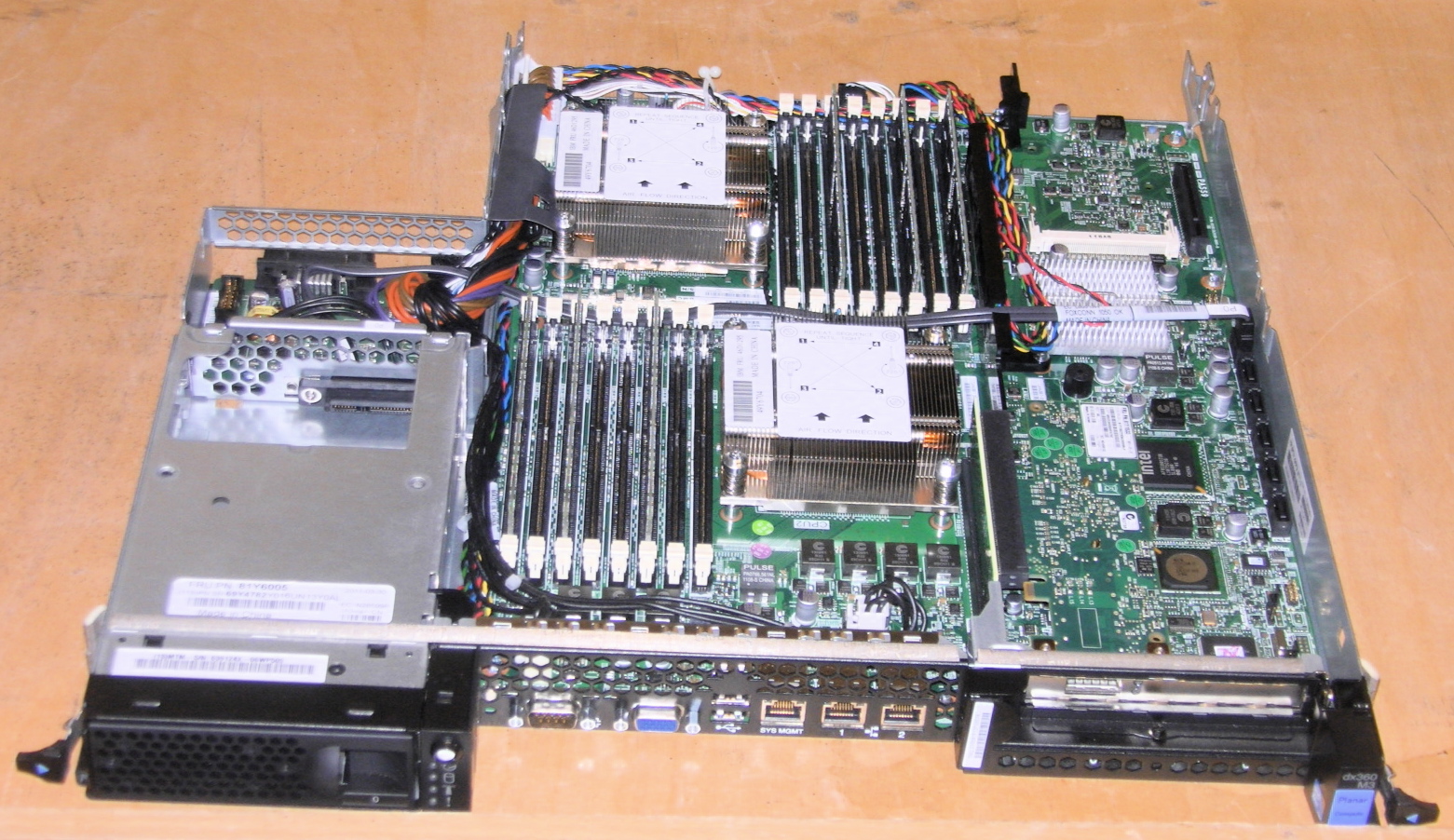
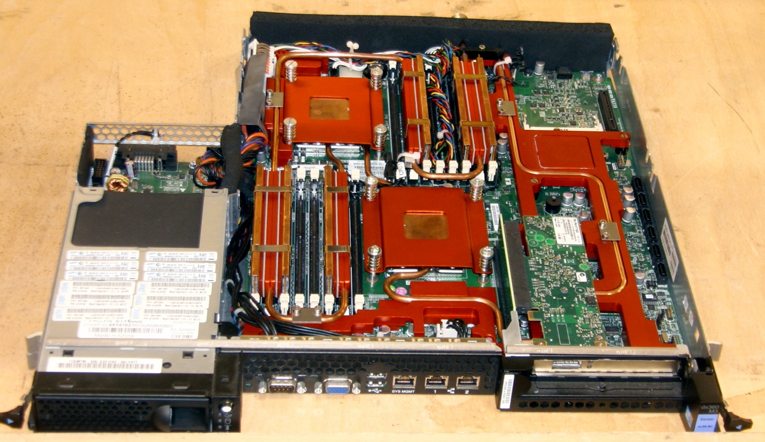
Figure 1: Left: Original air-cooled iDataPlex dx360 M3 compute node. The power supply unit (not shown) is attached to the compute node on the top left. Right: iDataCool compute node with new water-cooling solution, consisting of a copper pipeline, copper heat sinks for processors and memory, and aluminium heat bridges. Armaflex thermal insulation is used to prevent heat from escaping into the environment.

Before presenting our liquid-cooling solution we briefly describe the iDataCool HPC cluster, which is based on the IBM System x iDataPlex architecture [10]. It consists of three racks with 72 compute nodes each. A compute node is equipped with either two four-core Intel Xeon E5630 (44 in total) or two six-core Intel Xeon E5645 (388 in total) Westmere processors organized as a distributed shared memory system. Each node contains 24 GB of memory arranged in six 4 GB DDR3 dual in-line memory modules. The main interconnect network of iDataCool is based on QDR Infiniband, arranged in a hybrid ring/tree topology. Switched Gigabit Ethernet is used for disk I/O, system booting via NFS, and job scheduling. Every compute node is monitored and controlled by a dedicated baseboard management controller (BMC).

The air-cooling components of the original iDataPlex system were completely removed and replaced by a custom water-cooling solution, shown in Fig. 1, which was developed in a joint effort of the University of Regensburg and the IBM Research and Development Lab Böblingen and manufactured and installed in the machine shop of the Regensburg Physics Department. The main design drivers of the water-cooling solution were the possibility of hot-water cooling and low cost. Let us focus on the first point for now. CPUs can tolerate a certain maximum chip temperature, which depends on the specific chip used. Thus, to enable high cooling-water temperatures, the temperature difference between the compute cores and the water should be minimized. The heat transfer path can be divided into two segments. First, the heat is transferred from the cores to the package surface. Second, the heat is transferred from the package surface to the cooling water via thermal interface material and a heat sink. We have no control over the first segment but can optimize the second one, in particular through the design of the processor heat sink, which is shown in Fig. 2. Its design parameters were as follows.

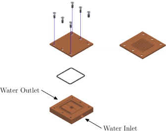
Figure 2: Design of the iDataCool heat sink. The top part, which is attached to the processor package, is shown from both sides.

• Minimize the temperature difference between coolant and processor package. This was achieved by bringing the coolant very close to the package and by using a material with high thermal conductivity, i.e., copper. (For the thermal interface material between heat sink and processor package we used Shin-Etsu X23-7783D.)

• Efficient thermal transport. This was achieved by the design shown in Fig. 2, which provides a sufficiently large interface area for heat transfer and creates turbulent flow.

• Low pressure drop. The channels shown in Fig. 2 are not microchannels but 1 mm wide. At a typical flow rate of 0.6 l/min the pressure drop is less than 0.1 bar.

• Low cost. The design shown in Fig. 2 is very simple and can be manufactured inexpensively with standard tools since the channels are rather wide. Using an O-ring and screws is simpler and more leak-proof than using glue.

The processor heat sinks are hard-soldered to a copper pipeline that provides the water flow. Other heat-critical components on the board are thermally coupled to the pipeline via copper or aluminum heat bridges and thermal interface material. These components include memory modules, Infiniband daughter card, chip set, voltage regulators, and several other chips. All of these components can tolerate higher temperatures than the processors. Different materials and designs are used to satisfy the cooling needs of these parts. E.g., the memory modules are cooled via copper heat bridges clamped to aluminum bars which embrace the cooling pipeline. Thus the memory modules can easily be replaced in the field. Proper mounting (including thermal interface material) and alignment of all components of the cooling solution is crucial for a high cooling performance.

Heat dissipation into the environment of the compute node is reduced using Armaflex thermal insulation. The only components of iDataCool that are still air-cooled are the power supply units and the network switches.

Only a minor modification of the node chassis was required to connect the cooling pipeline, via inexpensive standard water connectors, to a rack-level manifold. The nodes are connected to the manifold in a parallel fashion. The manifold is designed using the Tichelmann principle to ensure that the distance covered by the water flow, and therefore the pressure drop, is equal for all nodes. Thus the water flow rates balance themselves automatically. The manifold is attached to the backside of each rack. Armaflex thermal insulation reduces the dissipation of heat from the pipes into the computing center.

An important issue is the cost of the liquid-cooling solution. All components are made from standard materials (copper, aluminum, plastic) and were designed such that the manufacturing process is simple, and thus inexpensive. There are only six soldering joints per node (two at each heat sink, and one each at the in- and outlet), and the bending of the copper pipe can be automated by a properly designed tool. The mounting of the liquid-cooling solution (including application of thermal interface material) was somewhat time-consuming, but on an industrial scale this process could also be automated. For us the total cost of the liquid-cooling solution was about 120 Euro per node (excluding external infrastructure). While this is more expensive than an air-cooled solution, it is a small fraction of the overall cost and can be amortized quickly by the savings from free cooling and energy reuse. On an industrial scale the costs would probably be even lower.

Our sensing and monitoring facilities are described at the beginning of Sect. 4.

3 Infrastructure

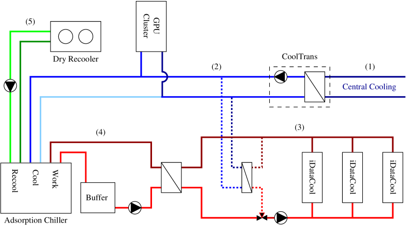
Figure 3: Liquid-cooling installation consisting of central cooling circuit (1), primary cooling circuit (2), rack cooling circuit (3), driving circuit (4), and recooling circuit (5).

iDataCool is installed in the computing center of Regensburg University, which was entirely air-cooled before. The liquid-cooling infrastructure for iDataCool was prepared in 2011 and completed in 2012. Since the spring of 2012 the waste heat of iDataCool drives an adsorption chiller (LTC 09 by InvenSor), which in turn generates chilled water. The LTC 09 is a so-called low-temperature chiller that works efficiently already at driving temperatures of around 65^∘C/149^∘F, see the efficiency curves in the data sheet [11]. The cooling performance of the chiller is balanced against the cooling needs of a small-sized GPU cluster that is cooled by the LTC 09. The GPU cluster has a peak power consumption of 12kW. The equipment of the GPU cluster is housed in a closed cabinet and cooled by air. The air is cooled by an air-water heat exchanger (Knürr CoolLoop [12]) that transfers the heat inside the cabinet to the water circuit.

Fig. 3 shows a schematic overview of the liquid-cooling installation. It consists of five water circuits. Each circuit is driven by a dedicated pump that keeps the water flow at a constant rate. Energy losses to the environment are reduced by thermal insulation of the hot parts of the plumbing. Special additives are used to minimize the risk of corrosion. In the following we discuss the details of the five circuits.

• The computing center is connected to the university’s central cooling circuit (1) which delivers chilled water at temperatures around 8^∘C/46^∘F.

• The primary cooling circuit (2) is continuously chilled by the adsorption chiller and picks up heat from the GPU cluster. In addition, the primary circuit can be used as an additional cooler for the iDataCool cluster, see the dotted lines in the figure. (A dry recooler would also suit this purpose.) If the water temperature exceeds 20^∘C/68^∘F the primary circuit is supported by the central cooling circuit (1), to which it is connected via a commercial heat exchanger that works autonomously (Knürr CoolTrans [13]).

• The iDataCool cluster is cooled by the rack cooling circuit (3) with hot water at outlet temperatures of up to $70^{\circ}$C/158^∘F. The waste heat of iDataCool is supplied to the driving circuit of the adsorption chiller (4) via a heat exchanger. Transfer of excess heat to the primary cooling circuit (2) allows us to keep the rack inlet temperature constant (even under change of load on the cluster). The heat transfer to primary and driving circuit is continuously regulated by a 3-way valve. The valve is automatically operated by a PID controller that determines the rack inlet temperature.

• The adsorption chiller is driven by the driving circuit (4). Temperature fluctuations in the driving circuit due to the operational characteristics of the chiller are smoothed by a buffer tank with a capacity of 800 liters. Due to proper thermal insulation there is virtually no temperature loss at the interface to the rack cooling circuit.

• The recooling circuit (5) connects to a fan-driven dry recooler that is located outside the computing center. The fans are controlled automatically by the adsorption chiller with the fan speed optimized for energy-efficient operation of the chiller. Evaporative cooling is possible in principle but has not been implemented in our setup. Freezing of the external recooling circuit is avoided by an admixture of ethylene glycol.

The standard use case of the adsorption chiller is rather different from our setup. Normally the chiller drives an air-conditioning system, i.e., one specifies the desired temperature of the chilled water, and the chiller then absorbs as much heat as necessary from the driving circuit to deliver the required cooling power. In our case we want the chiller to absorb the heat from the rack circuit and to deliver as much cooling power as possible. To see how this works we now discuss in some detail the behavior of our system. The chiller is characterized by its cooling capacity $P_{c}^{\text{max}}$, which is the maximum amount of heat per unit time it can remove from the cooling circuit, and by its coefficient of performance, defined as

$$\text{COP}=\frac{\text{power}\;P_{c}\;\text{removed from cooling circuit}}{\text{power}\;P_{d}^{\text{abs}}\;\text{absorbed from driving circuit}}\;.$$

All of these quantities depend (among other parameters) on the temperature $T$ in the driving circuit [11]. Now assume that the 3-way valve in Fig. 3 completely shuts off the additional cooling path and that we turn on the iDataCool cluster with an initial water temperature of, say, 20^∘C/68^∘F. At $T<55^{\circ}$C/131^∘F the adsorption chiller is in standby mode and thus absorbs no heat from the cluster. As a result, the temperature in the rack circuit increases until it goes above 55^∘C/131^∘F and the chiller turns on. What happens then depends on the temperature dependence of the function $P_{d}^{\text{max}}(T)=P_{c}^{\text{max}}(T)/\text{COP}(T)$, which is the maximum power that can be removed from the driving circuit of the chiller. This function depends on the parameters of the chiller. A certain power $P_{d}$ is transferred from the rack circuit to the driving circuit. If $P_{d}^{\text{max}}(T)<P_{d}$ the temperature keeps going up. If $P_{d}^{\text{max}}(T)$ intersects $P_{d}$ at some $T=T_{\text{eq}}$, the system settles into equilibrium at that temperature. If $P_{d}$ is larger than the maximum of $P_{d}^{\text{max}}(T)$, we have to employ the additional cooling mechanism via the 3-way valve to remove the rest of the heat and to keep the rack circuit at a well-defined temperature. The parameters of our system are such that for $T=60\ldots 70^{\circ}$C/$140\ldots 158^{\circ}$F the value of $P_{d}^{\text{max}}(T)$ is almost equal to, but slightly smaller than, the power transferred from the rack circuit to the driving circuit at maximum load of the cluster. Thus the system is almost in equilibrium and only a very small amount of additional cooling is necessary.

Our setup also solves two redundancy issues: (i) Should the adsorption chiller fail to absorb all the heat from the iDataCool cluster, additional cooling is provided by the primary cooling circuit, which may be supported by the central cooling circuit. (ii) Should the adsorption chiller fail to provide enough cooling power to the GPU cluster, again the central cooling circuit comes to the rescue.

4 Measurements

In this section we present a number of measurements and benchmarks performed on the iDataCool system. We first describe our sensing and monitoring facilities. The liquid-cooling installation is constantly monitored, and relevant system parameters are logged electronically. On the node level, we read out the individual processor core temperatures from chip-internal sensors, we estimate the water in- and outlet temperature of each node using the original air-flow temperature sensors (which we attached to the copper pipe), and we monitor the DC power consumption of each node. On the cluster level, we measure the in- and outlet temperature and the AC power consumption of the 3-rack installation. Our instrumentation also allows us to determine the combined AC power consumption of the iDataCool cluster, the GPU cluster, water pumps, the adsorption chiller, and the dry recooler. To determine the flow rates in the different water circuits we use various kinds of flow meters. As for the accuracy of our equipment, we estimate the node-level temperature sensors to be accurate to about 1^∘C/2^∘F, while the cluster-level temperature sensors, which are in direct contact with the water, are specified to have an accuracy of 0.2^∘C/0.4^∘F. The ultrasonic flow meter for the rack cooling circuit is specified to have an accuracy of 1%, while the flow meters for the other circuits are much simpler and only about 10% accurate.

When plotting quantities as a function of the cooling-water temperature we have the choice of using the rack inlet or outlet temperature. We chose the outlet temperature $T_{\text{out}}$ since this is the quantity of interest for energy reuse purposes. The difference between inlet and outlet temperature can be controlled by adjusting the water flow rate and is about 5^∘C/9^∘F in our system. For constant rack inlet temperature, $T_{\text{out}}$ fluctuates slightly depending on the load of the cluster and on the control parameters. In the figures, the horizontal error bars in the $T_{\text{out}}$ direction reflect these fluctuations in time.

Some of our measurements [those presented in Figs. 4(a), 5(a), and 6(a)] were taken on a subset of 13 randomly selected nodes (six-core E5645 processors at 2.4 GHz with Turbo Boost disabled) running a well-defined load (the standard stress tool [14]). The other measurements were taken on the whole iDataCool system running in production mode, i.e., various jobs of different sizes and with different computing and communication requirements are scheduled and executed by the batch queueing system.

(a)

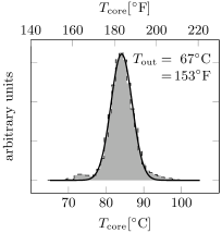
(b)

Figure 4: 4(a) Core temperatures of 13 compute nodes under stress and 4(b) core temperature distribution of the cluster in production mode. In both plots only six-core E5645 processors are included. The vertical error bars in 4(a) are the standard deviations after averaging over time and nodes.

In Fig. 4(a) we show the average compute core temperature as a function of the outlet temperature. The average difference between core and water temperature increases slightly, from 15^∘C/59^∘F to 17.5^∘C/63.5^∘F, over the range of temperatures considered. The error bars are rather large, indicating a large variation between nodes. A histogram of core temperatures for $T_{\text{out}}=67^{\circ}$C/153^∘F is shown in Fig. 4(b). The solid line is a Gaussian fit centered at $84^{\circ}$C/183^∘F with $\sigma=2.8^{\circ}$C/5.0^∘F. The small bump at the low end of the histogram is due to idle nodes that have a much lower core temperature. Our interpretation of the large spread visible in Fig. 4(b) is that it is mainly due to the first segment of the heat transfer path described in Sect. 2, over which we have no control, while we can control the second part very carefully. Nevertheless, this spread is a real problem if we aim, with energy reuse in mind, for a high outlet temperature. The cores throttle at about 100^∘C/212^∘F, so the outlet temperature is limited by the core with the largest difference between core and outlet temperature. In our system this largest difference is below 30^∘C/54^∘F so that we can safely run at $T_{\text{out}}\leq 70^{\circ}$C/158^∘F. If we desired higher temperatures we could sort out the “bad” chips and run them at lower temperature in a separate system. The high end of the histogram in Fig. 4(b) indicates that we could perhaps gain another 5^∘C/9^∘F in this way.

(a)

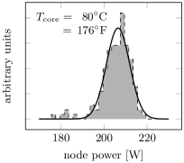
(b)

Figure 5: 5(a) Node power consumption of 13 compute nodes under stress and 5(b) node power distribution of the cluster in production mode. In both plots only six-core E5645 processors are included.

The power consumption per node also shows large fluctuations. In Fig. 5(a) we present the DC power consumption of 13 nodes vs. their average core temperature. To quantify the spread we measure the DC power on most six-core nodes for various temperatures, interpolate to $80^{\circ}$C/176^∘F, and then construct a histogram of the interpolated node power, see Fig. 5(b). The solid line is a Gaussian fit centered at 206W with $\sigma=5.4$W. We see that the individual CPUs vary greatly in their power consumption even for the same coolant temperature. We again attribute most of these variations to the manufacturing process of the chips, not to our liquid-cooling solution.

(a)

(b)

Figure 6: 6(a) Relative node power increase for 13 nodes with six-core E5645 processors and 6(b) COP of adsorption chiller. The vertical error bars in 6(a) are the standard deviations after averaging over nodes, while the vertical error bars in 6(b) reflect the 10% accuracy of the flow meters.

With higher cooling-water temperatures the power consumption of the nodes increases, which has a negative effect on the total energy reuse efficiency of the system. To quantify this effect we plot in Fig. 6(a) the relative average increase of the node power consumption, which is about 7% when going from 49^∘C/120^∘F to 70^∘C/158^∘F. This should be compared to the efficiency gain of the adsorption chiller, which is quantified by the COP defined in Sect. 3 and shown in Fig. 6(b). The temperature in the last plot starts at 57^∘C/135^∘F since the adsorption chiller is in standby mode for lower temperatures. When going from 57^∘C/135^∘F to 70^∘C/158^∘F the COP increases by 90%, while the node power consumption increases by only 5%. Thus the energy reuse efficiency dramatically improves when running at higher temperatures.

In Fig. 7(a) we show the fraction of the electric power delivered to the cluster that is transferred to the water in the rack circuit. We observe that this fraction drastically decreases with temperature. The reason for this decrease is the imperfect thermal insulation of the iDataCool racks from the environment. A higher temperature difference between rack and air implies that more energy is lost to the air. The lesson from this figure is that in future hot-water cooling designs serious attention should be paid to the thermal insulation of the rack already in the early planning stages. In Fig. 7(b) we show the fraction of electric power that is transferred to the driving circuit of the adsorption chiller, i.e., $P_{d}/P_{\text{electric}}$, as a function of the coolant temperature in the rack circuit. The increase shows that higher coolant temperatures in the rack circuit lead to a better utilization of the chiller, i.e., for our system the increase of the chiller effectiveness with $T_{\text{out}}$ outweighs the reduced heat in water.

(a)

(b)

Figure 7: 7(a) Heat-in-water fraction and 7(b) transferred power. The vertical error bars in 7(a) combine temporal fluctuations of the inlet- and outlet coolant temperatures and the flow, while the vertical error bars in 6(b) reflect the 10% accuracy of the flow meters.

We do not show plots of the fraction of energy reused (or, equivalently, of the energy reuse efficiency) since the cooling capacity of our chiller is not high enough to convert all heat from the iDataCool system to chilled water. The fraction of energy that could be reused (e.g., by adding another chiller) can be computed by multiplying the numbers in Figs. 6(b) and 7(a) and is on the order of 25% for $T=60\ldots 70^{\circ}$C/140…158^∘F. With better thermal insulation this fraction could increase by almost a factor of two at $T=70^{\circ}$C/158^∘F, see Fig. 7(a).

5 Conclusions

We have demonstrated that, by employing a sophisticated but low-cost water-cooling solution, it is possible to cool a large compute cluster in stable production mode with water outlet temperatures of up to 70^∘C/158^∘F. At such temperatures a significant fraction of the energy consumed by the cluster can be reused. In the iDataCool system the waste heat from the cluster drives an adsorption chiller that operates efficiently above 65^∘C/149^∘F. The minor increase in power consumption of the nodes due to the higher temperature is more than offset by the dramatic increase in the COP of the chiller.

The main problem of the iDataCool system is the imperfect thermal insulation, which leads to a serious loss of heat to the environment and decreases the amount of energy that can be reused. In future designs this problem should be attacked from the very start. Our numbers indicate that with better thermal insulation almost 50% of the energy can be recovered in the form of chilled water. Of course, other opportunities for energy reuse exist where an even higher fraction of the energy can be recovered, e.g., by heating. However, at some sites heating may not be an option or not necessary at all, in which case the generation of chilled water, which can be used to cool other parts of the computing center, is an attractive possibility.

Finally, an important issue is the effect of high water temperatures on the reliability of electronic components, and in general on the long-term stability of the system. iDataCool gives us a unique opportunity to study this issue (except for hard disks since the iDataCool nodes are diskless). We cannot predict the future, but after more than one year of cooling with hot water we have not yet observed any negative effects.

References

- [1] IDC White Paper #231528, Server Transition Alternatives: A Business Value View Focusing on Operating Costs, (2012)
- [2] H. Coles, M. Elsworth, D.J. Martinez, “Hot” for Warm Water Cooling, SC ’11 State of the Practice Reports, Article No. 17, ACM, New York (2011)
- [3] N. Meyer et al., Data centre infrastructure requirements, European Exascale project DEEP (2012)
- [4] S. Zimmermann et al., Aquasar: A hot water cooled data center with direct energy reuse, Energy 43 (2012) 237
- [5] A. Auweter and H. Huber, Direct warm water cooled Linux Cluster Munich: CoolMUC, inSiDE 10 (2012) 26
- [6] H. Baier et al., QPACE: Power-efficient parallel architecture based on IBM PowerXCell 8i, Computer Science - Research and Development 25 (2010) 149
- [7] Eurotech, AURORA Liquid Cooling Solution, http://www.eurotech.com/aurora
- [8] Clustered Systems Company (P. Hughes), Liquid Cooling for Servers, Server Design Summit (2011)
- [9] LRZ, SuperMUC Petascale System, http://www.lrz.de/supermuc
- [10] IBM System x iDataPlex dx360 M3, http://www-03.ibm.com/systems/x/hardware/rack/dx360m3/index.html
- [11] InvenSor GmbH Germany, LTC 09 adsorption chiller data sheet, http://www.invensor.com/en/pdf/Datasheet_Invensor_LTC_09.pdf
- [12] Knürr AG Germany, CoolLoop data sheet, http://www.emersonnetworkpower.com/en-EMEA/Brands/Knurr/Documents/en/brochures/CoolLoop.pdf
- [13] Knürr AG Germany, CoolTrans data sheet, http://www.emersonnetworkpower.com/en-EMEA/Brands/Knurr/Documents/en/brochures/CoolTrans.pdf
- [14] http://weather.ou.edu/~apw/projects/stress