Fisher–Hartwig expansion for the transverse correlation function
in the XX spin-1/2 chain

Abstract

Motivated by the recent results on the asymptotic behavior of Toeplitz determinants with Fisher–Hartwig singularities, we develop an asymptotic expansion for transverse spin correlations in the XX spin-1/2 chain. The coefficients of the expansion can be calculated to any given order using the relation to discrete Painlevé equations. We present explicit results up to the eleventh order and compare them with a numerical example.

I Introduction

The spin-1/2 XX chain described by the Hamiltonian

$$H=\sum_{i=-\infty}^{+\infty}\left[-J(\sigma^{x}_{i}\sigma^{x}_{i+1}+\sigma^{y}_{i}\sigma^{y}_{i+1})+h\sigma^{z}_{i}\right]$$ (1)

(where $\sigma^{\alpha}_{i}$ are Pauli matrices associated with the spin at the site $i$) is one of the simplest examples of exactly solvable spin systems: by a Jordan–Wigner transformation it can be mapped onto free fermions, which gives a complete solution for the ground state and for the excitations lieb:61 (this model is also equivalent to the Tonks–Girardeau gas of hard-core bosons on a one-dimensional lattice girardeau:60 ). Computing correlation functions is, however, a more difficult task, since transverse spin operators (or, equivalently, the boson operators in the Tonks–Girardeau gas) are nonlocal in terms of fermions. In particular, already the leading-order asymptotic behavior of the ground-state transverse correlations

$$\langle\sigma^{+}_{i}\sigma^{-}_{i+L}\rangle\propto L^{-1/2}\,,\qquad L\to\infty$$ (2)

requires a nontrivial calculation BosLead . One of the possible approaches to this correlation function is to re-express it as a Toeplitz determinant of a Fisher–Hartwig type by using the fermionic representation lieb:61 ; schultz:63 ; mccoy:68 . The asymptotic behavior of such determinants continues to be an object of active studies in mathematics and mathematical physics fisher:68 ; basor:94 ; ehrhardt:01 ; basor:06 ; kozlowski:08:09:10 ; calabrese:10 ; gutman:11 ; deift:11 ; krasovsky:11 . In particular, some corrections to the leading asymptotic behavior of the correlation function (2) have been computed vaidya:79 ; jimbo:80 ; creamer:81 ; gangardt:04:06 ; note-vaidya .

In the present paper we extend this approach by demonstrating that all the corrections to Eq. (2) can be computed order by order using the recent results on a closely related Toeplitz determinant for statistics of free fermions ivanov:13-1 ; ivanov:13-2 . Furthermore, those corrections may be combined into a double sum explicitly periodic in the “counting parameter” (Eqs. (14)–(15) below): this double-sum form was dubbed Fisher–Hartwig expansion in Ref. ivanov:13-2, .

Note that while our calculation can be performed analytically to any order, it does not constitute a rigorous proof: in fact, the results of Refs. ivanov:13-1, ; ivanov:13-2, on which it is based still have a status of conjecture. The available analytical and numerical evidence calabrese:10 ; abanov:11 ; suesstrunk:12 ; ivanov:13-2 leaves no doubt in the validity of this conjecture (see a more detailed discussion of this in Section V), however we find it helpful to check our analytical results against numerical evaluations of the determinants. Such a check provides an additional support to the conjecture and verifies analytical manipulations performed with Mathematica software Wolfram (see Section IV for detail).

The paper is organized as follows. In Section II, we report our analytical results on the Fisher–Hartwig expansion of the relevant Toeplitz determinant. In Section III we apply these results to the case of transverse spin correlations in the XX chain. In Section IV, we compare the analytical results with a numerical example. Finally, in Section V we discuss the assumptions used in our calculation and the implications of our results. The Appendix contains expressions for some of the expansion coefficients.

II Main results

The Hamiltonian (1) can be diagonalized via the Jordan–Wigner transformation lieb:61

$$\sigma^{+}_{i} =\Psi^{\dagger}_{i}\exp\left(i\pi\sum_{j<i}\Psi^{\dagger}_{j}\Psi_{j}\right)\,,$$

$$\sigma^{-}_{i} =\exp\left(i\pi\sum_{j<i}\Psi^{\dagger}_{j}\Psi_{j}\right)\Psi_{i}\,,$$ (3)

$$\sigma^{z}_{i} =2\,\Psi^{\dagger}_{i}\Psi_{i}-1\,.$$

In terms of the fermionic operators $\Psi^{\dagger}_{i}$ and $\Psi_{i}$, the Hamiltonian (1) represents free spinless fermions on a one-dimensional lattice with $J$ being the hopping amplitude and $h$ corresponding to the chemical potential. The ground state of such a system is a Fermi sea where all the states below the Fermi wave vector $k_{F}=\arccos(h/2J)$ are filled (here we assume that $|h|<2J$: otherwise the ground state is a trivial fully polarized state corresponding to $k_{F}=0$ or $k_{F}=\pi$). The parameter $k_{F}$ ranges between $0$ and $\pi$ and fully describes the ground state. The average density of fermions in the ground state is $k_{F}/\pi$, which corresponds to $\langle\sigma_{i}^{z}\rangle=2k_{F}/\pi-1$.

We will be interested in the transverse spin correlation function (2). For our purposes, it will be more convenient to introduce a more general correlation function involving a “counting parameter” $\kappa$:

$$\Sigma(\kappa,k_{F},L)=\left\langle\Psi^{\dagger}_{0}\exp\left(2\pi i\kappa\sum_{1\leq j\leq L-1}\Psi^{\dagger}_{j}\Psi_{j}\right)\Psi_{L}\right\rangle\,,$$ (4)

where the average is taken over the ground state in an infinite system. Then, by the Jordan–Wigner transformation, the transverse spin correlation function is a particular case of this definition:

$$\langle\sigma^{+}_{i}\sigma^{-}_{i+L}\rangle=\Sigma\left(\kappa{=}\frac{1}{2},k_{F},L\right)\,.$$ (5)

Note that $\Sigma(\kappa,k_{F},L)$ is explicitly periodic in $\kappa$ with period one, since the number of fermions $\sum_{1\leq j\leq L-1}\Psi^{\dagger}_{j}\Psi_{j}$ is integer.

Using the Wick theorem, the correlation function (4) can be expressed as lieb:61 ; schultz:63

$$\Sigma(\kappa,k_{F},L)=\\ =(1-e^{2\pi i\kappa})^{-1}\det_{1\leq i,j\leq L}\left[\left(1-e^{2\pi i\kappa}\right)a_{i-j+1}-\delta_{i-j+1}\right]\,,$$ (6)

where

$$a_{i-j}=\left\langle\Psi^{\dagger}_{i}\Psi_{j}\right\rangle=\begin{cases}\frac{\sin k_{F}(i-j)}{\pi(i-j)}\,,&i\neq j\,,\\ k_{F}/\pi\,,&i=j\end{cases}$$ (7)

and

$$\delta_{i-j}=\begin{cases}0\,,&i\neq j\,,\\ 1\,,&i=j\end{cases}$$ (8)

The determinant in Eq. (6) is very similar to that studied in Ref. ivanov:13-2, for the correlation function

$$\chi(\kappa,k_{F},L)=\left\langle\exp\left(2\pi i\kappa\sum_{1\leq j\leq L}\Psi^{\dagger}_{j}\Psi_{j}\right)\right\rangle\\ =\det_{1\leq i,j\leq L}\left[\left(e^{2\pi i\kappa}-1\right)a_{i-j}+\delta_{i-j}\right]\,.$$ (9)

Namely, up to an overall sign, the Toeplitz matrices (6) and (9) differ only by a shift by one row (or, equivalently, by one column). The determinants of such Toeplitz matrices may therefore be related using the Desnanot-Jacobi identity muir:06 ; brualdi:83 (also known as the Lewis Carroll identity dodgson:66 , which is a particular case of the Muir relations muir:83 ):

$$[\chi(\kappa,k_{F},L)]^{2}-[(1-e^{2\pi i\kappa})\Sigma(\kappa,k_{F},L)]^{2}\\ =\chi(\kappa,k_{F},L-1)\,\chi(\kappa,k_{F},L+1)\,.$$ (10)

This relation determines $\Sigma(\kappa,k_{F},L)$ up to a sign, once $\chi(\kappa,k_{F},L)$ is known. The sign of $\Sigma(\kappa,k_{F},L)$ may, in turn, be fixed independently from the known main asymptotics (2) note-xL .

We can now use the asymptotic expansion for $\chi(\kappa,k_{F},L)$ derived in Ref. ivanov:13-2, :

$$\chi(\kappa,k_{F},L)=\sum_{j=-\infty}^{+\infty}\chi_{*}(\kappa+j,k_{F},L)\,,$$ (11)

where

$$\chi_{*}(\kappa,k_{F},L)=\exp\Big{[}2i\kappa k_{F}L-2\kappa^{2}\ln(2L\sin k_{F})\\ +{\tilde{C}}(\kappa)+\sum_{n=1}^{\infty}{\tilde{F}}_{n}(\kappa,k_{F})\,(iL)^{-n}\Big{]}\,,$$ (12)

$${\tilde{C}}(\kappa)=2\ln[G(1+\kappa)G(1-\kappa)]\,,$$ (13)

$G()$ is the Barnes G function, and ${\tilde{F}}_{n}(\kappa,k_{F})$ are some polynomials in $\kappa$ and $\cot k_{F}$.

By re-expressing $\Sigma(\kappa,k_{F},L)$ from the relation (10), we arrive at a similar asymptotic expression,

$$\Sigma(\kappa,k_{F},L)=\left(1-e^{2\pi i\kappa}\right)^{-1}\sqrt{\frac{2\sin k_{F}}{L}}\\ \times\sum_{j=-\infty}^{+\infty}\Sigma_{*}(\kappa+j+\frac{1}{2},k_{F},L)\,,$$ (14)

where

$$\Sigma_{*}(\bar{\kappa},k_{F},L)=\exp\Big{[}2i\bar{\kappa}k_{F}L-2\bar{\kappa}^{2}\ln(2L\sin k_{F})\\ +C_{\Sigma}(\bar{\kappa})+\sum_{n=1}^{\infty}H_{n}(\bar{\kappa},k_{F})\,(iL)^{-n}\Big{]}\,,$$ (15)

and

$$C_{\Sigma}(\bar{\kappa})=\ln[G(\frac{3}{2}+\bar{\kappa})G(\frac{1}{2}+\bar{\kappa})G(\frac{1}{2}-\bar{\kappa})G(\frac{3}{2}-\bar{\kappa})]\,.$$ (16)

We use the notation $\bar{\kappa}$ for the variables in Eqs. (15) and (16) to emphasize that this variable is shifted by a half-integer from the original variable $\kappa$. The coefficients $H_{n}(\bar{\kappa},k_{F})$ can be calculated from the coefficients ${\tilde{F}}_{n}(\kappa,k_{F})$ order by order. We have calculated the first ten orders using Mathematica software Wolfram . The first six coefficients are:

$$H_{1}(\bar{\kappa},k_{F}) =\left(\bar{\kappa}^{2}-\frac{1}{4}\right)\cdot 2\bar{\kappa}\cot k_{F}$$

$$H_{2}(\bar{\kappa},k_{F}) =\left(\bar{\kappa}^{2}-\frac{1}{4}\right)\left[\left(\frac{5}{2}\bar{\kappa}^{2}-\frac{1}{8}\right)\cot^{2}k_{F}+\frac{4}{3}\bar{\kappa}^{2}\right]$$

$$H_{3}(\bar{\kappa},k_{F}) =\left(\bar{\kappa}^{2}-\frac{1}{4}\right)\bigg{[}\left(\frac{11}{2}\bar{\kappa}^{3}-\frac{3}{8}\bar{\kappa}\right)\cot^{3}k_{F}$$

$$+\left(\frac{9}{2}\bar{\kappa}^{3}-\frac{1}{8}\bar{\kappa}\right)\cot k_{F}\bigg{]}$$

$$H_{4}(\bar{\kappa},k_{F}) =\left(\bar{\kappa}^{2}-\frac{1}{4}\right)\bigg{[}\left(\frac{63}{4}\bar{\kappa}^{4}-\frac{11}{16}\bar{\kappa}^{2}-\frac{1}{16}\right)\cot^{4}k_{F}$$

$$+\left(\frac{35}{2}\bar{\kappa}^{4}+\frac{1}{8}\bar{\kappa}^{2}-\frac{1}{8}\right)\cot^{2}k_{F}$$

$$+\frac{167}{60}\bar{\kappa}^{4}+\frac{29}{80}\bar{\kappa}^{2}-\frac{1}{32}\bigg{]}$$

$$H_{5}(\bar{\kappa},k_{F}) =\left(\bar{\kappa}^{2}-\frac{1}{4}\right)$$

$$\times\bigg{[}\left(\frac{527}{10}\bar{\kappa}^{5}+\frac{17}{10}\bar{\kappa}^{3}-\frac{23}{32}\bar{\kappa}\right)\cot^{5}k_{F}$$

$$+\left(74\bar{\kappa}^{5}+7\bar{\kappa}^{3}-\frac{11}{8}\bar{\kappa}\right)\cot^{3}k_{F}$$

$$+\left(\frac{45}{2}\bar{\kappa}^{5}+\frac{9}{2}\bar{\kappa}^{3}-\frac{17}{32}\bar{\kappa}\right)\cot k_{F}\bigg{]}$$

$$H_{6}(\bar{\kappa},k_{F}) =\left(\bar{\kappa}^{2}-\frac{1}{4}\right)$$

$$\times\bigg{[}\left(\frac{3129}{16}\bar{\kappa}^{6}+\frac{6271}{192}\bar{\kappa}^{4}-\frac{3599}{768}\bar{\kappa}^{2}-\frac{539}{3072}\right)\cot^{6}k_{F}$$

$$+\left(\frac{2655}{8}\bar{\kappa}^{6}+\frac{2563}{32}\bar{\kappa}^{4}-\frac{1155}{128}\bar{\kappa}^{2}-\frac{223}{512}\right)\cot^{4}k_{F}$$

$$+\left(\frac{2385}{16}\bar{\kappa}^{6}+\frac{3341}{64}\bar{\kappa}^{4}-\frac{1021}{256}\bar{\kappa}^{2}-\frac{353}{1024}\right)\cot^{2}k_{F}$$

$$+\frac{236}{21}\bar{\kappa}^{6}+\frac{781}{126}\bar{\kappa}^{4}-\frac{17}{504}\bar{\kappa}^{2}-\frac{1}{16}\bigg{]}$$ (17)

The coefficients $H_{7}(\bar{\kappa},k_{F})$ to $H_{10}(\bar{\kappa},k_{F})$ are listed in the Appendix.

The expansion (14)–(15), together with the algorithm for computing the coefficients $H_{n}(\bar{\kappa},k_{F})$ [starting from the coefficients ${\tilde{F}}_{n}(\kappa,k_{F})$], constitutes the main result of the present work. The algorithm for calculating ${\tilde{F}}_{n}(\kappa,k_{F})$ using discrete Painlevé equations was reported earlier in Ref. ivanov:13-2, . Combined together, these results provide an algorithm for calculating the expansion for $\Sigma(\kappa,k_{F},L)$ to any given order. The transverse spin correlations can be obtained by setting $\kappa=1/2$ in all the formulas (so that the summation in the expansion (14)–(15) is performed over all integer $\bar{\kappa}$).

We note several properties of the coefficients $H_{n}(\bar{\kappa},k_{F})$. Similarly to ${\tilde{F}}_{n}(\kappa,k_{F})$, they are polynomials in $\bar{\kappa}$ and $\cot k_{F}$ with rational coefficients. These polynomials have degrees $(n+2)$ and $n$ in $\bar{\kappa}$ and $\cot k_{F}$, respectively and are of a fixed parity in each of these variables (even for even $n$ and odd for odd $n$). Moreover, they are all divisible by $(\bar{\kappa}^{2}-1/4)$: this property must persist to all orders, since it guarantees that the expansion (14)–(15) reproduces the fermionic correlation function (7) in the limit $\kappa\to 0$.

III Transverse spin correlations in the XX chain

We now specify to the case of the transverse spin correlation function (5). In this case, all the powers of $L^{-1}$ in the expansion (14)–(15) are integer, and the expansion may be rewritten in the form

$$\langle\sigma^{+}_{i}\sigma^{-}_{i+L}\rangle=e^{C_{\Sigma}(0)}\sqrt{\frac{\sin k_{F}}{2L}}\\ \times\sum_{j=-\infty}^{+\infty}(2\sin k_{F})^{-2j^{2}}e^{2i\,j\,k_{F}L}\sum_{n=0}^{\infty}\frac{\alpha_{jn}(k_{F})}{(iL)^{n}}\,.$$ (18)

This form of expansion has already been established in Ref. vaidya:79, . The coefficients $\alpha_{jn}(k_{F})$ can be calculated in a simple manner from the coefficients $H_{n}(\bar{\kappa},k_{F})$. Note that at any given order $n$, the coefficients $\alpha_{jn}(k_{F})$ are nonzero only for $|j|\leq\sqrt{n/2}$. The explicit form of the coefficients $\alpha_{jn}(k_{F})$ for $n$ up to 11 is given in Appendix.

The beginning of the expansion (18) reads

$$\langle\sigma^{+}_{i}\sigma^{-}_{i+L}\rangle=e^{C_{\Sigma}(0)}\sqrt{\frac{\sin k_{F}}{2L}}\\ \times\Bigg{(}1-\frac{\cos^{2}k_{F}+4\cos(2k_{F}L)}{32(L\sin k_{F})^{2}}\\ -\frac{3\cos k_{F}\,\sin(2k_{F}L)}{16(L\sin k_{F})^{3}}+\ldots\Bigg{)}\,.$$ (19)

The leading order gives the asymptotic behavior (2) with the correct coefficient vaidya:79 ; jimbo:80 ; creamer:81 ; gangardt:04:06 :

$$e^{C_{\Sigma}(0)}=\left[G(1/2)G(3/2)\right]^{2}=2^{1/6}e^{1/2}A^{-6}\,,$$ (20)

where $A=1.2824271291\ldots$ is the Glaisher-Kinkelin constant. The subsequent coefficients $\alpha_{jn}$ reproduce, in particular, the corrections calculated in Refs. creamer:81, ; gangardt:04:06, .

IV Numerical illustration

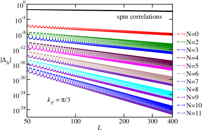
Figure 1: The difference $\Delta_{N}$ between the left-hand side of Eq. (18) and its right-hand side with the sum over $n$ restricted to $n\leq N$ is plotted as a function of $L$. The value of $k_{F}$ is $\pi/3$. The upper line is the spin correlations [the left-hand side of Eq. (18)], and the other data correspond, top to bottom, to $N=0$ to $N=11$ [excluding $N=1$, since there are no first-order terms in the expansion (18)].

We illustrate our analytic calculation with a numerical example of the correlation function (5). We have chosen the Fermi wave vector $k_{F}=\pi/3$ (corresponding to the $z$ polarization equal to $1/3$ of the full polarization) and have numerically calculated the corresponding determinants for distance $L$ up to 400. In our numerics, we have used the LAPACK library lapack:99 compiled to work with 128-bit floating-point numbers, together with the quadmath C library.

In Fig. 1 we plot the difference $\Delta_{N}(k_{F},L)$ between the left-hand side of Eq. (18) and its right-hand side with the sum over $n$ restricted to $n\leq N$. These results show that, even though our analytical calculations involved a non-rigorous analytic continuation of the asymptotic series to half-integer values of $\kappa$, such an analyticity, in fact, holds. A similar conclusion was also reached in Refs. calabrese:10, ; abanov:11, ; suesstrunk:12, ; ivanov:13-2, for the expansion of $\chi(\kappa,k_{F},L)$.

V Discussion

In the present paper, we apply the earlier results of Ref. ivanov:13-2, on the Toeplitz determinants with the sine kernel to deriving a Fisher–Hartwig expansion for the correlation function (4) [including, the transverse spin correlations (5) as a particular case]. The expansion is not rigorously proven and remains a conjecture supported by several arguments.

Away from the line $\operatorname{Re}\kappa=j+1/2$ (with an integer $j$), this expansion may be verified order by order using the methods of Refs. calabrese:10, ; ivanov:13-2, (and of Ref. ivanov:13-1, in the continuous limit $k_{F}\to 0$). The verification was actually performed to the tenth order in the lattice case and to the fifteenth order in the continuous limit, and this leaves little doubt about the validity of the general form of the expansion to all orders.

On the line $\operatorname{Re}\kappa=j+1/2$ (relevant for the case of the transverse correlations in the XX model), the situation is more delicate. In this case, the expansion cannot even be rigorously derived to any order, but is obtained by an analytic continuation from other values of $\kappa$. This is not a mathematically justified procedure, and therefore our results at $\operatorname{Re}\kappa=j+1/2$ are additionally based on the assumption that the expansion (11)–(12) of $\chi(\kappa,k_{F},L)$ is analytically continuable, term by term, across the line $\operatorname{Re}\kappa=j+1/2$ (see Refs. ivanov:13-1, ; ivanov:13-2, ). The corresponding analytic continuation for the expansion (14)–(15) of $\Sigma(\kappa,k_{F},L)$ follows from this assumption, together with the Lewis Carroll identity (10). At this point it is not clear how to prove this assumption. However, available numerical studies (Refs. calabrese:10, ; abanov:11, ; suesstrunk:12, ; ivanov:13-2, and this paper) indicate that, in the examples and to the orders considered, the analytic continuation of the expansions to the line $\operatorname{Re}\kappa=j+1/2$ is indeed possible.

These conjectures present a challenge to future mathematical studies of Toeplitz determinants. Besides proving them, an interesting question remains if they are valid for other Toeplitz determinants with Fisher–Hartwig singularities, or, even more generally, for pseudo-differential operators with discontinuous symbols sobolev:10 . Transferring some of the results on the Fisher–Hartwig expansion to spectral properties of such operators would have implications in extending the Widom conjecture widom:82 to a wider class of functions. In particular, this may lead to extracting subleading corrections to the von Neumann entanglement entropy for free fermions in higher dimensions (similarly to the one-dimensional case suesstrunk:12 ; ivanov:13-2 ).

Another use of the present results may be in application to one-dimensional bosonization (describing the low-energy fermionic degrees of freedom in terms of bosonic fields) stone:94 . While the subleading bosonization terms (responsible for the discreteness of fermionic particles) are model dependenthaldane:81 , it might be possible to fix them for the specific model (free fermions on a chain) by using expansions for correlation functions obtained from Toeplitz determinants.

Appendix

The coefficients $H_{n}(\bar{\kappa},k_{F})$ in orders seven to ten are:

$$H_{7}(\bar{\kappa},k_{F}) =\left(\bar{\kappa}^{2}-\frac{1}{4}\right)$$

$$\times\bigg{[}\bigg{(}\frac{175045}{224}\bar{\kappa}^{7}+\frac{257105}{896}\bar{\kappa}^{5}$$

$$-\frac{51889}{3584}\bar{\kappa}^{3}-\frac{8243}{2048}\bar{\kappa}\bigg{)}\cot^{7}k_{F}$$

$$+\bigg{(}\frac{49755}{32}\bar{\kappa}^{7}+\frac{90319}{128}\bar{\kappa}^{5}$$

$$-\frac{10991}{512}\bar{\kappa}^{3}-\frac{21563}{2048}\bar{\kappa}\bigg{)}\cot^{5}k_{F}$$

$$+\bigg{(}\frac{88735}{96}\bar{\kappa}^{7}+\frac{202627}{384}\bar{\kappa}^{5}$$

$$-\frac{35}{1536}\bar{\kappa}^{3}-\frac{18261}{2048}\bar{\kappa}\bigg{)}\cot^{3}k_{F}$$

$$+\bigg{(}\frac{4765}{32}\bar{\kappa}^{7}+\frac{14281}{128}\bar{\kappa}^{5}+\frac{3031}{512}\bar{\kappa}^{3}-\frac{4669}{2048}\bar{\kappa}\bigg{)}\cot k_{F}\bigg{]}\,,$$

$$H_{8}(\bar{\kappa},k_{F}) =\left(\bar{\kappa}^{2}-\frac{1}{4}\right)$$

$$\times\bigg{[}\bigg{(}\frac{422565}{128}\bar{\kappa}^{8}+\frac{1079589}{512}\bar{\kappa}^{6}+\frac{235859}{2048}\bar{\kappa}^{4}$$

$$-\frac{407593}{8192}\bar{\kappa}^{2}-\frac{10045}{8192}\bigg{)}\cot^{8}k_{F}$$

$$+\bigg{(}\frac{723283}{96}\bar{\kappa}^{8}+\frac{2134807}{384}\bar{\kappa}^{6}+\frac{659881}{1536}\bar{\kappa}^{4}$$

$$-\frac{281377}{2048}\bar{\kappa}^{2}-\frac{1945}{512}\bigg{)}\cot^{6}k_{F}$$

$$+\bigg{(}\frac{356807}{64}\bar{\kappa}^{8}+\frac{1234703}{256}\bar{\kappa}^{6}+\frac{545033}{1024}\bar{\kappa}^{4}$$

$$-\frac{520155}{4096}\bar{\kappa}^{2}-\frac{17025}{4096}\bigg{)}\cot^{4}k_{F}$$

$$+\bigg{(}\frac{44825}{32}\bar{\kappa}^{8}+\frac{186653}{128}\bar{\kappa}^{6}+\frac{121011}{512}\bar{\kappa}^{4}$$

$$-\frac{83617}{2048}\bar{\kappa}^{2}-\frac{1865}{1024}\bigg{)}\cot^{2}k_{F}$$

$$+\frac{353777}{5760}\kappa^{8}+\frac{1874177}{23040}\bar{\kappa}^{6}+\frac{1954679}{92160}\bar{\kappa}^{4}$$

$$-\frac{252007}{122880}\bar{\kappa}^{2}-\frac{1697}{8192}\bigg{]}\,,$$

$$H_{9}(\bar{\kappa},k_{F}) =\left(\bar{\kappa}^{2}-\frac{1}{4}\right)$$

$$\times\bigg{[}\bigg{(}\frac{1398251}{96}\bar{\kappa}^{9}+\frac{2759869}{192}\bar{\kappa}^{7}+\frac{263645}{96}\bar{\kappa}^{5}$$

$$-\frac{383007}{1024}\bar{\kappa}^{3}-\frac{365609}{8192}\bar{\kappa}\bigg{)}\cot^{9}k_{F}$$

$$+\bigg{(}\frac{149997}{4}\bar{\kappa}^{9}+\frac{329653}{8}\bar{\kappa}^{7}+\frac{144741}{16}\bar{\kappa}^{5}$$

$$-\frac{135021}{128}\bar{\kappa}^{3}-\frac{150545}{1024}\bar{\kappa}\bigg{)}\cot^{7}k_{F}$$

$$+\bigg{(}\frac{2656689}{80}\bar{\kappa}^{9}+\frac{6574367}{160}\bar{\kappa}^{7}+\frac{424443}{40}\bar{\kappa}^{5}$$

$$-\frac{2573727}{2560}\bar{\kappa}^{3}-\frac{719261}{4096}\bar{\kappa}\bigg{)}\cot^{5}k_{F}$$

$$+\bigg{(}11414\bar{\kappa}^{9}+\frac{64723}{4}\bar{\kappa}^{7}+\frac{81147}{16}\bar{\kappa}^{5}$$

$$-\frac{21975}{64}\bar{\kappa}^{3}-\frac{22669}{256}\bar{\kappa}\bigg{)}\cot^{3}k_{F}$$

$$+\bigg{(}\frac{36597}{32}\bar{\kappa}^{9}+\frac{122547}{64}\bar{\kappa}^{7}+\frac{24549}{32}\bar{\kappa}^{5}$$

$$-\frac{21459}{1024}\bar{\kappa}^{3}-\frac{123653}{8192}\bar{\kappa}\bigg{)}\cot k_{F}\bigg{]}\,,$$

$$H_{10}(\bar{\kappa},k_{F}) =\left(\bar{\kappa}^{2}-\frac{1}{4}\right)$$

$$\times\bigg{[}\bigg{(}\frac{266149}{4}\bar{\kappa}^{10}+\frac{60326939}{640}\bar{\kappa}^{8}+\frac{44195357}{1280}\bar{\kappa}^{6}$$

$$-\frac{181763}{320}\bar{\kappa}^{4}-\frac{17390113}{20480}\bar{\kappa}^{2}-\frac{2645371}{163840}\bigg{)}\cot^{10}k_{F}$$

$$+\bigg{(}\frac{381511}{2}\bar{\kappa}^{10}+\frac{588149}{2}\bar{\kappa}^{8}+\frac{15122545}{128}\bar{\kappa}^{6}$$

$$-\frac{142507}{512}\bar{\kappa}^{4}-\frac{6068297}{2048}\bar{\kappa}^{2}-\frac{494569}{8192}\bigg{)}\cot^{8}k_{F}$$

$$+\bigg{(}\frac{786877}{4}\bar{\kappa}^{10}+\frac{21302633}{64}\bar{\kappa}^{8}+\frac{19058315}{128}\bar{\kappa}^{6}$$

$$+\frac{9023}{4}\bar{\kappa}^{4}-\frac{7867861}{2048}\bar{\kappa}^{2}-\frac{1402057}{16384}\bigg{)}\cot^{6}k_{F}$$

$$+\bigg{(}\frac{344253}{4}\bar{\kappa}^{10}+\frac{5177563}{32}\bar{\kappa}^{8}+\frac{657703}{8}\bar{\kappa}^{6}$$

$$+\frac{810981}{256}\bar{\kappa}^{4}-\frac{2264409}{1024}\bar{\kappa}^{2}-\frac{457181}{8192}\bigg{)}\cot^{4}k_{F}$$

$$+\bigg{(}\frac{27937}{2}\bar{\kappa}^{10}+\frac{3807047}{128}\bar{\kappa}^{8}+\frac{4528105}{256}\bar{\kappa}^{6}$$

$$+\frac{5181}{4}\bar{\kappa}^{4}-\frac{2064369}{4096}\bar{\kappa}^{2}-\frac{512839}{32768}\bigg{)}\cot^{2}k_{F}$$

$$+\frac{264031}{660}\bar{\kappa}^{10}+\frac{1055183}{1056}\bar{\kappa}^{8}+\frac{15531919}{21120}\bar{\kappa}^{6}$$

$$+\frac{2831703}{28160}\bar{\kappa}^{4}-\frac{492119}{22528}\bar{\kappa}^{2}-\frac{2301}{2048}\bigg{]}\,.$$ (21)

We also list all nonzero coefficients $\alpha_{jn}(k_{F})$ for $n\leq 11$. Only coefficients with $j\geq 0$ are presented because of the symmetry $\alpha_{-jn}(k_{F})=(-1)^{n}\alpha_{jn}(k_{F})$:

$$\alpha_{00}(k_{F}) =1\,,\qquad\alpha_{02}(k_{F})=\frac{1}{32}\cot^{2}k_{F}\,,$$

$$\alpha_{12}(k_{F}) =\frac{1}{4}\,,\qquad\alpha_{13}(k_{F})=\frac{3}{8}\cot k_{F}\,,$$

$$\alpha_{04}(k_{F}) =\frac{33}{2048}\cot^{4}k_{F}+\frac{1}{32}\cot^{2}k_{F}+\frac{1}{128}\,,$$

$$\alpha_{14}(k_{F}) =\frac{93}{128}\cot^{2}k_{F}+\frac{1}{4}\,,$$

$$\alpha_{15}(k_{F}) =\frac{453}{256}\cot^{3}k_{F}+\frac{153}{128}\cot k_{F}\,,$$

$$\alpha_{06}(k_{F}) =\frac{2907}{65536}\cot^{6}k_{F}+\frac{225}{2048}\cot^{4}k_{F}$$

$$+\frac{177}{2048}\cot^{2}k_{F}+\frac{1}{64}\,,$$

$$\alpha_{16}(k_{F}) =\frac{42633}{8192}\cot^{4}k_{F}+\frac{1341}{256}\cot^{2}k_{F}+\frac{363}{512}\,,$$

$$\alpha_{17}(k_{F}) =\frac{293895}{16384}\cot^{5}k_{F}+\frac{98325}{4096}\cot^{3}k_{F}$$

$$\hskip 28.45274pt+\frac{7011}{1024}\cot k_{F}\,,$$

$$\alpha_{08}(k_{F}) =\frac{2584107}{8388608}\cot^{8}k_{F}+\frac{1953}{2048}\cot^{6}k_{F}$$

$$+\frac{273267}{262144}\cot^{4}k_{F}+\frac{467}{1024}\cot^{2}k_{F}+\frac{849}{16384}\,,$$

$$\alpha_{18}(k_{F}) =\frac{18582471}{262144}\cot^{6}k_{F}+\frac{970029}{8192}\cot^{4}k_{F}$$

$$\hskip 14.22636pt+\frac{428337}{8192}\cot^{2}k_{F}+\frac{1985}{512}\,,$$

$$\alpha_{28}(k_{F}) =\frac{9}{256}\,,$$

$$\alpha_{19}(k_{F}) =\frac{165603555}{524288}\cot^{7}k_{F}+\frac{165851145}{262144}\cot^{5}k_{F}$$

$$\hskip 14.22636pt+\frac{12465711}{32768}\cot^{3}k_{F}+\frac{2052147}{32768}\cot^{k}_{F}\,,$$

$$\alpha_{29}(k_{F}) =\frac{135}{256}\cot k_{F}\,,$$

$$\alpha_{0,10}(k_{F}) =\frac{1086306255}{268435456}\cot^{10}k_{F}+\frac{63442485}{4194304}\cot^{8}k_{F}$$

$$\hskip 14.22636pt+\frac{44944731}{2097152}\cot^{6}k_{F}+\frac{3662175}{262144}\cot^{4}k_{F}$$

$$\hskip 14.22636pt+\frac{1026407}{262144}\cot^{2}k_{F}+\frac{1151}{4096}\,,$$

$$\alpha_{1,10}(k_{F}) =\frac{52562685915}{33554432}\cot^{8}k_{F}$$

$$+\frac{1918340595}{524288}\cot^{6}k_{F}+\frac{2927324961}{1048576}\cot^{4}k_{F}$$

$$+\frac{48020019}{65536}\cot^{2}k_{F}+\frac{4529519}{131072}\,,$$

$$\alpha_{2,10}(k_{F}) =\frac{43065}{8192}\cot^{2}k_{F}+\frac{45}{64}\,,$$

$$\alpha_{1,11}(k_{F}) =\frac{574231373145}{67108864}\cot^{9}k_{F}$$

$$+\frac{191554621335}{8388608}\cot^{7}k_{F}+\frac{44340529815}{2097152}\cot^{5}k_{F}$$

$$+\frac{8076485685}{1048576}\cot^{3}k_{F}+\frac{219859155}{262144}\cot k_{F}\,,$$

$$\alpha_{2,11}(k_{F}) =\frac{368685}{8192}\cot^{3}k_{F}+\frac{62505}{4096}\cot k_{F}\,.$$ (22)

References

• (1) E. Lieb, T. Schultz, and D. Mattis, Ann. Phys. 16, 407 (1961).
Two soluble models of an antiferromagnetic chain.
• (2) M. Girardeau, J. Math. Phys. 1, 516 (1960).
Relationship between systems of impenetrable bosons and fermions in one dimension.
• (3) Probably, the easiest way of deriving the leading term (2) is to use the bosonization technique luther:75 .
• (4) T. D. Schultz, J. Math. Phys. 4, 666 (1963).
Note on the one-dimensional gas of impenetrable point-particle bosons.
• (5) B. M. McCoy, Phys. Rev. 173, 531 (1968).
Spin Correlation Functions of the X-Y Model.
• (6) M. E. Fisher and R. E. Hartwig, Adv. Chem. Phys. 15, 333 (1968).
Toeplitz determinants, some applications, theorems and conjectures.
• (7) E. L. Basor, K. E. Morrison, Linear Algebra Appl. 202, 129 (1994)
The Fisher-Hartwig conjecture and Toeplitz eigenvalues.
• (8) T. Ehrhardt, Operator Theory: Adv. Appl. 124, 217 (2001).
A status report on the asymptotic behavior of Toeplitz determinants with Fisher-Hartwig singularities.
• (9) E. Basor, Toeplitz Determinants and Statistical Mechanics, in “Encyclopedia of Mathematical Physics”, Elsevier, vol. 5, 244 (2006).
• (10) K. K. Kozlowski, arXiv:0805.3902.
Truncated Wiener–Hopf operators with Fisher Hartwig singularities.
N. Kitanine, K. K. Kozlowski, J. M. Maillet, N. A. Slavnov, and V. Terras, Comm. Math. Phys. 291, 691 (2009).
Riemann–Hilbert approach to a generalized sine kernel and applications.
N. Kitanine, K. K. Kozlowski, J. M. Maillet, N. A. Slavnov, and V. Terras, J. Stat. Mech.: The. and Exp. , P04033 (2009).
Algebraic Bethe ansatz approach to the asymptotic behavior of correlation functions.
K. K. Kozlowski, arXiv:1011.5897.
Riemann–Hilbert approach to the time-dependent generalized sine kernel.
• (11) P. Calabrese and F. H. L. Essler, J. Stat. Mech., P08029 (2010).
Universal corrections to scaling for block entanglement in spin-1/2 XX chains.
• (12) D. B. Gutman, Y. Gefen, and A. D. Mirlin, J. Phys. A: Math. Theor. 44, 165003 (2011),
Non-equilibrium 1D many-body problems and asymptotic properties of Toeplitz determinants.
• (13) P. Deift, A. Its, and I. Krasovsky, Ann. of Math. 174, 1243 (2011).
Asymptotics of Toeplitz, Hankel, and Toeplitz + Hankel determinants with Fisher-Hartwig singularities.
• (14) I. Krasovsky, Aspects of Toeplitz determinants, in “Boundaries and Spectra of Random Walks” (eds. D. Lenz, F. Sobieczky, W. Woess), Progr. Probability 64, 305 (2011).
• (15) H. G. Vaidya and C. A. Tracy, Phys. Rev. Lett. 42, 3 (1979).
One-particle reduced density matrix of impenetrable bosons in one dimension at zero temperature.
H. G. Vaidya and C. A. Tracy, J. Math. Phys. 20, 2291 (1979).
One particle reduced density matrix of impenetrable bosons in one dimension at zero temperature.
• (16) M. Jimbo, T. Miwa, Y. Môri, and M. Sato, Physica D 1, 80 (1980).
Density matrix of an impenetrable Bose gas and the fifth Painlevé transcendent.
• (17) D. B. Creamer, H. B. Thacker, and D. Wilkinson, Phys. Dev. D 23, 3081 (1981).
Some exact results for the two-point function of an integrable quantum field theory.
• (18) D. M. Gangardt, J. Phys. A: Math. Gen. 37, 9335 (2004).
Universal correlations of trapped one-dimensional impenetrable bosons.
D. M. Gangardt and G. V. Shlyapnikov, New J. Phys. 8, 167 (2006).
Off-diagonal correlations of lattice impenetrable bosons in one dimension.
• (19) The expansion coefficients in Refs. vaidya:79, ; jimbo:80, contain typos which were corrected later in Refs. creamer:81, ; gangardt:04:06, .
• (20) D. A. Ivanov, A. G. Abanov, and V. V. Cheianov, J. Phys. A: Math. Theor. 46, 085003 (2013),
Counting free fermions on a line: a Fisher–Hartwig asymptotic expansion for the Toeplitz determinant in the double-scaling limit.
• (21) D. A. Ivanov and A. G. Abanov, arXiv:1306.5017.