On the nature of the brightest globular cluster in M81

Abstract

We analyse the photometric, chemical, star formation history and structural properties of the brightest globular cluster (GC) in M81, referred as GC1 in this work, with the intention of establishing its nature and origin. We find that it is a metal-rich ([Fe/H]=$-0.60\pm 0.10$), alpha-enhanced ([$\alpha/{\rm Fe}]\sim 0.20\pm 0.05$), core-collapsed (core radius $r_{c}=1.2$ pc, tidal radius $r_{t}=76r_{c}$), old ($>13$ Gyr) cluster. It has an ultraviolet excess equivalent of $\sim 2500$ blue horizontal branch stars. It is detected in X-rays indicative of the presence of low-mass binaries. With a mass of $1.0\times 10^{7}$ $M_{\odot}$, the cluster is comparable in mass to M31-G1 and is four times more massive than $\omega$ Cen. The values of $r_{c}$, absolute magnitude and mean surface brightness of GC1 suggest that it could be, like massive GCs in other giant galaxies, the left-over nucleus of a dissolved dwarf galaxy.

1 INTRODUCTION

The most massive globular clusters (GCs) (mass $\ga 2\times 10^{6}$ $M_{\odot}$) in galaxies are found to be different from the rest of the GC population in their physical, chemical and dynamical properties (Haşegan et al., 2005; Mieske et al., 2006; Georgiev et al., 2009; Taylor et al., 2010; Jang et al., 2012). These massive clusters seem to be related to the higher mass compact systems such as nuclear clusters (Georgiev et al., 2009) and ultra-compact dwarfs (UCDs) (Phillipps et al., 2001) rather than to the lower-mass classical GCs. Thus, it seems unlikely that the massive GCs were formed in-situ in the halos of their present parent galaxies, like their lower mass counterparts. Meanwhile, there is growing evidence in support of the idea proposed by Zinnecker et al. (1988), that was later tested using numerical simulations by Bekki & Freeman (2003), that some of the massive compact objects could be left-over nuclei of tidally stripped dwarf galaxies. Well-known examples of these type of clusters are $\omega$ Cen in our galaxy (Meylan et al., 1995), Mayall II (G1) in M31 (Meylan et al., 2001), and several massive GCs in NGC5128 (Taylor et al., 2010).

The brightest GC in a galaxy would also be the most massive if it is old like most GCs. GCs in elliptical galaxies all seem to be older than 10 Gyr (Brodie & Strader, 2006; Strader et al., 2005), the exception being the gas-rich elliptical NGC1316 which contains intermediate-age (3–10 Gyr) GCs (Goudfrooij et al., 2001). However, there is clear evidence of GC-like objects forming at present epochs in gas-rich spirals that have experienced merging (e.g. Antennae: Whitmore & Schweizer, 1995). Even mild interactions are able to trigger the formation of massive compact objects such as the case of M82, which has formed a population of compact clusters in its disk following its interaction with M81 around 500 Myr ago (Mayya et al., 2008; Konstantopoulos et al., 2009). It is not yet established whether this interaction or a similar interaction in the past was able to form any massive compact clusters in M81, that would have observational properties of old GCs.

In a systematic search for compact clusters in M81 using the HST/ACS images, Santiago-Cortés, Mayya, & Rosa-González (2010) identified R05R06584 (GC1 henceforth; RA=09:55:22.042 $\delta=+$69:06:37.84 (J2000)) as the brightest among the 172 GCs in this galaxy. It was noted in that work that the cluster is more luminous than the brightest GCs in the Milky Way ($\omega$ Cen) and Andromeda (M31-G1), the only two galaxies of comparable mass that are closer to us than M81. GC1 is seen at a projected galactocentric distance of only 3.0 kpc, as compared to galactocentric distances of 6.3 kpc, and 40 kpc of $\omega$ Cen and M31-G1, respectively. The object had been previously identified as 50777 in Perelmuter & Racine (1995) and was the target of a spectroscopic study by Nantais & Huchra (2010) (their object 1029), who reported a metallicity of [Fe/H]$=-0.86\pm 0.41$. They calculated this metallicity using emperical relations between Lick indices and metallicity (Brodie & Huchra, 1990). They also reported a radial velocity of $131\pm 5$ km s^-1, which is consistent with radial velocity obtained for disk objects at the observed galacto-centric distance of GC1.

In spite of being the brightest GC in M81, the nature of GC1 is unknown. If it is an old GC like $\omega$ Cen or M31-G1, it would be the most massive GC not only in M81, but also in the local Universe (distance $\lesssim 3.6$ Mpc). On the other hand, if it was formed later on, its mass would be smaller. Determination of its age is critical to distinguish these two possibilities. The cluster is not resolved into individual stars even on the HST/ACS images, and hence age cannot be obtained using the classical technique of colour-magnitude diagram (CMD). In this paper, we determine the age using two independent methods: (1) by fitting the optical spectrum between 3600–7000 Å with a model spectrum that is constructed as a sum of several Single Stellar Populations (SSPs) using the code STARLIGHT, and (2) by fitting the UV to MIR spectral energy distribution (SED) with SSPs of fixed ages. The latter method is very powerful in inferring the presence of intermediate-age populations (Bressan et al., 1998). In Table 1, we compare the absolute magnitude ($M_{V}$), metallicity ([Fe/H]), $V-I$ colour at the cluster center, age, mass, central $V$-band surface brightness ($\mu(0,V)$), and the structural parameters of GC1 to the corresponding parameters in $\omega$ Cen and M31-G1. The tabulated masses are photometric masses. Two additional values of masses are given for M31-G1 inside parentheses, both obtained using dynamical methods by Meylan et al. (2001), the smaller one is the Virial mass and the larger one is the King mass.

In §2, we describe observational data used in this work. The method we adopted to obtain the structural properties is given in §3. In §4, we describe the analysis technique we have used to obtain the metallicity, age, extinction and mass of GC1. The nature and the origin of GC1 are discussed in §5.

Table 1: Structural and physical properties of M81-GC1 compared to those in $\omega$ Cen and M31-G1.

Name	Mv(GC)	[Fe/H]	$(V-I)_{0}$	Age	Mass	$\mu(0,V)$	$c=\log(r_{t}/r_{c})$	rc	rh	$\epsilon$	Ref.1
	mag		mag	Gyr	$10^{6}$ $M_{\odot}$	mag arcsec-2		pc	pc
$\omega$ Cen	$-10.37$	$-1.62$	0.88	$>13$	2.3	14.38	0.98	3.58	7.71	0.17	(a,b)
M31-G1 (Mayall II)	$-10.90$	$-0.95$	1.10	$>13$	8.6(7.3,15)	13.47	2.50	0.52	13.5	0.20	(c,d)
M81-GC1 (R05R06584)	$-11.40$	$-0.60$	0.96	$>13$	10	14.93	1.88	1.23	5.60	0.12	(e,f)

¹ References are (a)Harris (1996), (b) Georgiev et al. (2009), (c)Meylan et al. (2001), (d) Ma et al. (2009), (e) Santiago-Cortés, Mayya, & Rosa-González (2010) and (f) this paper.

2 OBSERVATIONAL DATA

2.1 HST Imaging data

The imaging data that we used in this work to obtain the structural parameters come from the HST observations in the F435W, F606W and F814W filters (PI: Andreas Zezas). These images have a sampling of $0\aas@@fstack{\prime\prime}05~{}{\rm pix}^{-1}$ which at the distance of 3.63 Mpc to M81 (Freedman et al., 1994) corresponds to 0.88 pc ${\rm pix}^{-1}$. The spatial resolution in these images, measured as the Full Width at Half Maximum of the Point Spread Function (PSF), is 2.1 pixel (1.8 pc). The cluster is located at a projected distance of 3 kpc from the nucleus within 10° of the north-west major axis of M81, as illustrated in Figure 1. A blow-up of GC1 in a colour-composite HST image is also shown in this figure.

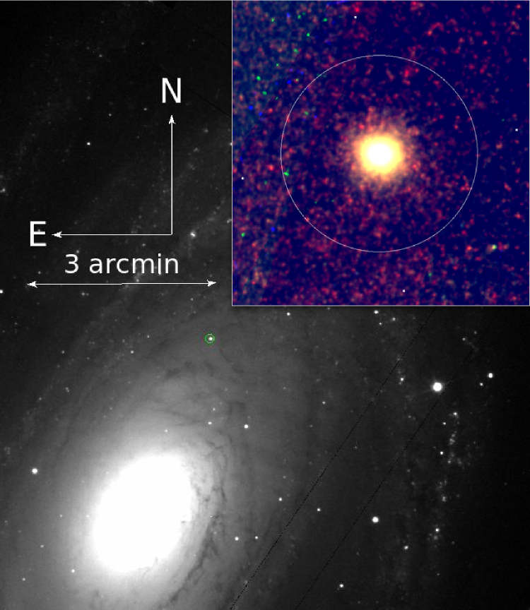
Figure 1: SDSS $g$-band image of M81 showing the location of GC1 with a circle. The inset contains an RGB image formed from the HST F814W (red), F606W (green) and F435W (blue) images. The circle around GC1 is of 4″ (75 pc) radius, which is the aperture used for multi-band photometry.

2.2 Spectroscopic observations

Spectroscopic observations were carried out using the long-slit of the spectrograph of the OSIRIS instrument at the 10.4-m GTC in the service mode on 2010 April 6. The observations included bias, flat fields, calibration lamps and standard star. A slit-width of 1″ was used and 3 exposures of 900 seconds each were realized, using the R1000B grism. The $2\times 1$ detector binning gives a spatial scale of 0.25 arcsec pix^-1, and spectral resolution of $\sim$7 Å  at 5510 Å. The seeing during the observations was $\sim 1\arcsec$.

The data reduction was carried out in the standard manner using the tasks available in the IRAF software package. The individual spectra were debiased, flat field and illumination corrected, wavelength calibrated and background subtracted. At the end of the reduction procedure, we combined the 3 different spectra and obtained a final spectrum free of cosmic rays. Observations of Feige 34 during the same night were used for flux calibration.

2.3 Multi-band photometric data

M81 was a target of the Spitzer Infrared Nearby Galaxies Survey (SINGS: Kennicutt et al. (2003); Pérez-González et al. (2006)). In addition to these mid infrared images, the galaxy was part of surveys at ultraviolet (Galex), optical (Sloan Digital Sky Survey; SDSS), and near infrared (2MASS) wavelengths. Fits format files from these missions are available at NED, which were used in this study.

2.3.1 Aperture photometry

We carried out aperture photometry on archival images in two Galex bands, five SDSS filters, the 2MASS JHK bands, the four bands of Spitzer/IRAC and the 24 $\mu$m band of Spitzer/MIPS. The object is clearly detected in all of these bands, except the 24 $\mu$m band, where we determined an upper limit. The relative isolation of the object allowed us to use an aperture of radius of 4″(75 pc) that is big enough to include more than 80% of the total flux in most bands. The aperture fluxes were multiplied by correction factors to account for the flux outside the aperture to obtain the total flux of GC1. The correction factor was more than 20% for the following three bands: 1.72 for Galex (NUV), 1.39 for Galex (FUV), and 1.22 for the 8 $\mu$m band of Spitzer/IRAC. For obtaining the aperture magnitudes, the sky was chosen in an annular region of 3″ width starting at 7″ radius. The instrumental magnitudes are converted into the system of ABmag (and Jansky) using the calibration constants in the headers of the respective images. Errors ($\delta F$) on the measured fluxes ($F$) are calculated as

$${\delta F\over{F}}={\sqrt{F+N\sigma_{\rm sky}^{2}T}\over{F\sqrt{T}}},$$ (1)

where $F$ is the count rate of photons measured in the aperture, $N$ is the number of pixels in the aperture, $\sigma_{\rm sky}$ the sky rms/second/pixel as measured in the part of the image outside the main galaxy, and $T$, the total exposure time in seconds in each image.

The multi-band integrated fluxes in ABMAGs and Janskys, along with their errors are given in Table 2.

Table 2: Multi-band integrated fluxes of GC1

$\lambda$	Mission/Filter	ABMAG	$F_{\nu}$	$\delta F_{\nu}/F_{\nu}$
Å		mag	Jy
1528	Galex-FUV	21.527	1.2367E-5	0.066
2271	Galex-NUV	21.239	1.9955E-5	0.034
3551	SDSS-u	18.861	1.0778E-4	0.023
4686	SDSS-g	17.257	4.5854E-4	0.002
6165	SDSS-r	16.551	8.9660E-4	0.002
7481	SDSS-i	16.158	1.2742E-3	0.001
8931	SDSS-z	15.846	1.7161E-3	0.005
12350	2MASS-J	15.595	2.2043E-3	0.024
16620	2MASS-H	15.480	2.4726E-3	0.027
21590	2MASS-K	15.820	1.7748E-3	0.034
35500	Spitzer-3.6	16.573	9.4611E-4	0.002
44900	Spitzer-4.5	17.081	5.9266E-4	0.003
57300	Spitzer-5.8	17.478	4.1880E-4	0.016
78700	Spitzer-8.0	18.367	1.9936E-4	0.037
236800	Spitzer-24	$>$20.570	$<$2.1478E-5	0.300

3 Determination of Structural Parameters

We used the IRAF/STSDAS software package ellipse to analyse the structural parameters of GC1 in the HST images. Ellipse is an algorithm designed to fit isophotes of galaxies with ellipses, where the intensity profiles decrease monotonically with radius. The first requirement of the analysis is to establish the best photometric centroid for the cluster. We started with the reported position of GC1 in Santiago-Cortés, Mayya, & Rosa-González (2010), which is the centroid defined by SExtractor (Bertin & Arnouts, 1996). We refined this centre by re-calculating the centre as the average centre of ellipses with semi-major axis $<5$ pixels. The resulting centre differed from that reported by Santiago-Cortés, Mayya, & Rosa-González (2010) by less than 1 pixel. However, we obtained surface brightness profiles by fixing the centre at this newly obtained value. Other quantities that affect the analysis of structural parameters are the choice of the background level and the range of radius used for fitting. We estimated the local background around GC1 in small ($10\times 10$ pixel²) boxes, and defined the fitting radius as the semi-major axis where the azimuthally averaged intensity reaches the previously measured background level. The cluster is devoid of any major contaminating sources in its immediate vicinity within 3″ radius that is considered in the analysis of the profiles — the nearest contaminating star is of $B=25.7$ mag (VEGAMAG) at a radial distance of 3$\aas@@fstack{\prime\prime}$26 (66 pixels) from the cluster centre. Finally, we subtracted the background value from the azimuthally averaged intensity profiles to obtain sky subtracted profiles in $F435W$ and $F814W$ bands.

We also analysed the variation of ellipticity ($\epsilon=1-\frac{b}{a}$) and the position angle of the major axis (PA) of the cluster for increasingly larger ellipses of fixed centres. The variation of $\epsilon$ and the PA as a function of semi-major axis length in $F435W$ and $F814W$ bands are shown in Figure 2. The PA and $\epsilon$ in the two filters remain almost constant between 5–20 pixels, at values of PA=$78.5\pm 5$° and $\epsilon=0.12\pm 0.02$. The values in the inner-most two pixels are limited by resolution and hence the observed differences in the two bands are not significant. The cluster is elongated almost along the perpendicular direction to the semi-major axis of the parent galaxy.

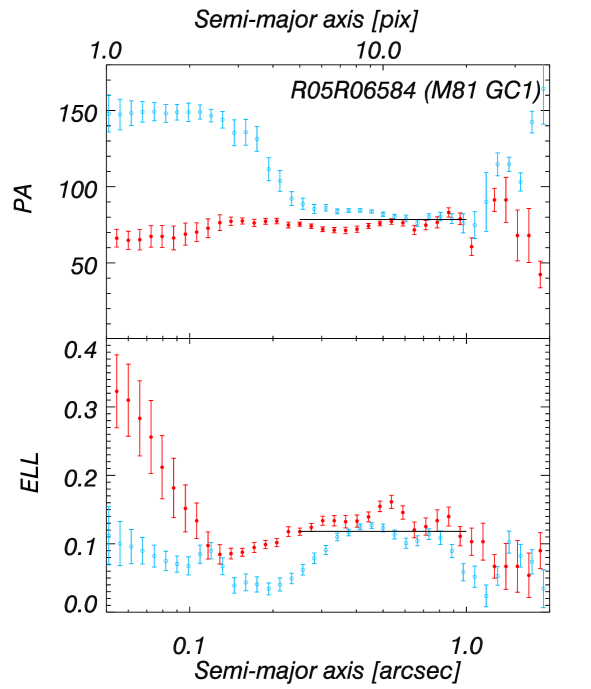
Figure 2: Variation of the ellipticity (bottom) and position angle (PA; measured from north to east) of the major axis (top) of the ellipses that best fit the isophotal intensities in $F435W$ (blue symbols) and $F814W$ (red symbols) bands. The values in both the bands remain constant between 5–20 pixels at values of PA=$78.5\pm 5$° and $\epsilon=0.12\pm 0.02$, which are shown by the horizontal bars in the corresponding panels.

The dynamical history of star clusters can be investigated through the analysis of their surface brightness profiles. It is well known that surface brightness profiles of most GCs in the Milky Way, M31 and M33 are reasonably well represented by the King model profile (King, 1962; McLaughlin & van der Marel, 2005). Consequently, we fit the radial intensity profile of GC1 with an empirical King model (King, 1962, 1966) after convolving it with the PSF of the image in each filter. The characteristic PSF was derived using the photometry routine IRAF/DAOPHOT using selected isolated stars uniformly distributed over the entire HST images that contain the GC1 star cluster in $F435W$ and $F814W$ bands. The procedure we followed to realize the fits is identical to that in ISHAPE (Larsen, 1999), except that our procedure allows the determination of the tidal radius $r_{t}$ directly from the fits.

The observed surface brightness profiles of CG1 in $F435W$ and $F814W$ bands are shown in Figure 3. Superposed on these observed profiles are the best fitting King model profiles (after convolving with the image PSFs). These models have core radius $r_{c}=1.80$ pix and tidal radius $r_{t}=146$ pix for the $F435W$ band, and $r_{c}=1.40$ pix and $r_{t}=106$ pix for the $F814W$ band. Whereas the King profile fits very well the observed profile over the entire plotted range in the $F814W$ band, the observed $F435W$-band central surface brightness is $\sim 1.0$ mag brighter than that for the best-fit King profile. This apparent ”blue core” is also seen in the colour profile (top panel), which is most likely related to the presence of blue horizontal branch stars that also produces an UV excess as discussed in §4.3. Thus, it is advisable not to use the blue-band profiles for obtaining structural parameters. Hence, we used the $r_{c}=1.40$ pix (1.2 pc) and $r_{t}=106$ pix (93 pc) for the $F814W$-band as typical values for GC1. This results in a value of $r_{t}/r_{c}=76$.

The ellipse task also performs photometry in successive ellipses. We used these photometric data to determine $R_{\rm eff}$, the radius where the aperture flux is half the total flux (also known as half-light radius $r_{h}$), in each of the two bands. The $R_{\rm eff}$ in the $F814W$ band is 5.6 pc. We also fitted a Moffatt model profile in both the filters. The King model fits the profiles better, especially in the outer parts.

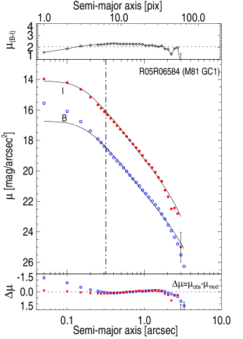
Figure 3: In the middle panel, the observed azimuthally averaged surface brightness profile for GC1 in the $F435W$ (empty circles) and $F814W$ (filled circles) bands, along with the best-fitting King profiles (solid lines) are shown. The vertical line represents the effective radius in the $F814W$ band. In the bottom panel, we show the residual (observed$-$King) surface brightness in $F435W$ (empty squares) and $F814W$ (filled squares) bands. Only the error bars with values greater than the symbol size are plotted. The $F435W-F814W$ colour profile is shown in the top panel, where the horizontal dashed line corresponds to the integrated colour of the cluster.

4 Determination of Physical parameters

4.1 New determination of [Fe/H] and [$\alpha$/Fe]

Figure 4: An illustration of the method used to determine [Fe/H] of GC1 from the 3 iron indices. The values for the Galactic GCs of Schiavon et al. (2005) (dots) are fitted with a polynomial of second order (solid line) to obtain a new emperical calibration. Observed values of indices for GC1 are plotted at their [Fe/H] values inferred from our emperical calibration, with the shaded area denoting our mean value of [Fe/H]$=-0.60\pm 0.10$. The [Fe/H] reported by Nantais & Huchra (2010) is shown by the filled square along with their error, on the left most panel. Our calibration not only has reduced the errors on the measurement, but also results in 0.26 dex higher metallicity.

Nantais & Huchra (2010) derived a metallicity [Fe/H]$=-0.86\pm 0.41$ for GC1 using empirical calibration of the indices defined by Brodie & Huchra (1990) and Trager et al. (1998) for Galactic GCs (Schiavon et al., 2005). Their value is the weighted mean of [Fe/H] values derived using indices MgH, Mg2, Mgb, F25270, Fe5335, Fe5406, G4300, $\delta$ and CNR, with more weights given to indices with larger dynamic range, defined as the ratio of sensitivity of the index (a change of 1 dex in [Fe/H]) to the observational error of the index. Such a weighting scheme doesn’t foresee variations of [$\alpha/Fe$] in GCs and hence would give erroneous values of [Fe/H] for systems that have [$\alpha/Fe$] values different from the mean value for the Galactic sample. The relatively large error in their measured value is an indicator of dispersion in the measured abundances using different indices. Low signal-to-noise ratio of their spectra may also be responsible for the large scatter.

We used our GTC spectra of GC1 to improve the value of [Fe/H] and also to newly determine the [$\alpha/Fe$]. We measured the indices Fe5270, Fe5335 and Fe5406 and determined the [Fe/H] as the mean of metallicities obtained from each of these indices as is illustrated in Figure 4. The [Fe/H] vs index data for the Galactic GCs of Schiavon et al. (2005) (dots) is fitted with a polynomial of second order (solid line) to obtain a new empirical calibration. Note that the fits clearly illustrate the quadratic nature of the relation, though it is a common practice to fit these points with a straight line (e.g. Nantais & Huchra, 2010). Observed values of indices for GC1 are plotted at the [Fe/H] values inferred from our empirical calibration, with the shaded area denoting our mean value of [Fe/H]$=-0.60\pm 0.10$. The [Fe/H] reported by Nantais & Huchra (2010) is shown by the filled square along with their error on the left most panel. Their large error bar is due to the use of non-iron indices to measure [Fe/H], and also the use of linear fits between indices and [Fe/H]. If we use our calibration of the three iron indices with the index values reported by them (Table 4 & Table 5 in their paper), we obtain [Fe/H]$=-0.48\pm 0.17$ which is in agreement with values from our spectra.

We also used the spectrum of GC1 to measure the Lick indices ratio Mgb/$<$Fe$>$ (Worthey et al., 1994), where $<$Fe$>=(Fe5270+Fe5335)/2.0$, and obtained the $\alpha$ element enhancement using the relation of Thomas et al. (2003). This gives us a value of $[\alpha/Fe]=0.20\pm 0.05$. Adopting the relation of Annibali et al. (2007) between the indices and metallicity, our observed values of [Fe/H] and $[\alpha/Fe]$ correspond to $Z=0.0056$ for the commonly used value of $Z\odot=0.02$. However, for the recently revised value of $Z\odot=0.014$ (Asplund et al., 2009), we get $Z=0.0043$.

4.2 Age of the Cluster from optical spectrum

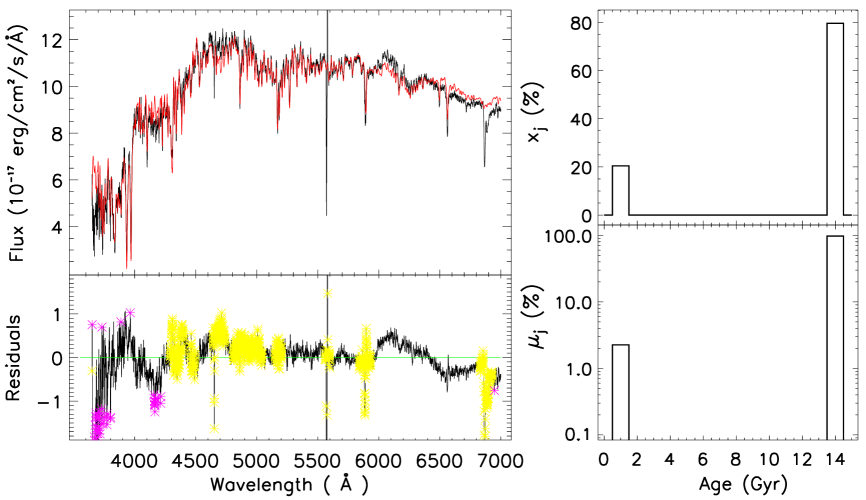
Figure 5: Results from the STARLIGHT analysis. The top left panel shows the best-fit model spectrum (red) overplotted on the observed spectrum (black). The residual spectrum in units of $10^{-17}$ erg cm² s^-1 Å^-1 is ploted at the bottom left panel, where the masked out regions are shown by yellow bands (emission lines) and pink asterics (bad pixels). The panels on the right show the star formation history of the cluster: top, the percentage in flux of different stellar populations at the reference wavelength (4020 Å), and the bottom, the percentage in mass, both as a function of age of the population. The stars that are formed $\gtrsim 13$ Gyr ago account for $\sim 98$% of the mass of the cluster.

We analysed our GTC spectrum of GC1 to determine the age of the stellar population, using the STARLIGHT spectral synthesis code (Cid Fernandes et al., 2005; Mateus et al., 2006). As a first step, we corrected the observed spectrum for Galactic extinction of $Av=0.22$ (maps of Schlegel (1998) and the reddening curve of Fitzpatrick (1999), using $R_{V}=3.1$). The spectrum was then brought to the rest frame wavelength, and also was resampled to pixels of 1Å between 3600 and 7000Å. The STARLIGHT decomposes an observed spectrum in to a number of simple stellar populations (SSPs), each of which contributes a fraction $x_{j}$ to the flux at a chosen normalization wavelength (in our case $\lambda_{0}$ = 4020 Å). We used 24 SSPs at a fixed metallicity of $Z=0.008$, the value closest to that observed in GC1 for which SSPs are available in STARLIGHT). The SSPs were extracted from the models of Bruzual & Charlot (2003), computed for a Salpeter (1955) initial mass function (IMF), “Padova-1994” evolutionary tracks (Alongi et al., 1993; Bressan et al., 1993; Fagotto et al., 1994a, b; Girardi et al., 1996), and STELIB library of observed stellar spectra (Le Borgne et al., 2003). The ages of these SSPs range from 1 Myr to 14 Gyr, at approximately logarithmic steps. Bad pixels and emission lines are masked and left out of the fits.

The results of the STARLIGHT analysis are shown in Figure 5. All the characteristics of the observed spectrum are very well reproduced by the fit, with the residuals well below 10% in most parts of the spectrum. In spite of using SSPs of 24 ages, we find nearly 98% of the stellar mass corresponding to stars that formed at the very early epochs of galaxy formation (age $>13$ Gyr) with an age spread $<2$ Gyr. The best-fit model suggests that around 20% of the blue light comes from another population — 1 Gyr old population of $\sim 2$% of total mass. In the next section, using the fits to the entire SED, we will show that the source of this blue excess is most likely, the extreme blue horizontal branch stars, that are not taken into account in the base SSPs in STARLIGHT, rather than a 1 Gyr old population. Thus, the optical spectrum of GC1 is consistent with an age of $\gtrsim$13 Gyr.

4.3 Age, Metallicity, Extinction and Cluster Mass from SED Analysis

The effects of the presence of dusty circumstellar envelopes around asymptotic giant branch (AGB) stars appear at wavelengths longward of a few microns and leave a clear excess around $10-15$ $\mu$m in the integrated mid-infrared (MIR) spectrum of passively evolving systems (Bregman et al., 1998; Bressan et al., 1998). Since AGB stars are luminous tracers of intermediate-age stellar populations, the presence or not of their characteristic MIR excess has been suggested as a powerful method to disentangle age and metallicity effects among these systems (Bressan et al., 1998, 2001, 2006). More specifically, the analysis of SSP models accounting for the effects of dusty AGB stars (Bressan et al., 1998) shows that a degeneracy between metallicity and age persists even in the MIR, since both age and metallicity affect mass-loss and evolutionary lifetimes on the AGB. While in the optical regime, age and metallicity need to be anti-correlated to maintain a feature unchanged (either colour or narrow-band index), in the MIR it is the opposite: the larger mass loss of a higher metallicity simple stellar population (SSP) must be balanced by its older age. Therefore, the detailed comparison of the MIR and optical data of passively evolving systems constitutes perhaps one of the cleanest ways to remove the degeneracy. The third parameter in the problem of the degeneracy is the extinction. In recent years, several studies (e.g. Bianchi et al., 2005; Kaviraj et al., 2007a; Bridžius et al., 2008; Rodríguez-Merino et al., 2011) have shown that the analysis of photometric data from the UV to the NIR spectral range help to disentangle the effects of reddening from those of evolution. However, they note that the derived metallicities do not reach the accuracies achievable by using spectroscopic data.

In this section, we follow the approach of the analysis of the panchromatic SED, with the innovation of having a wider spectral range, from the UV to the MIR, and by comparing these data with suitable SSP models accounting for the effects of dusty AGB stars (Bressan et al., 1998, 2012). Notice that the photometric data reported in Table 2 correspond to fluxes integrated over the entire cluster, which ensures reliable results from the analysis of SED.

As a first step, we corrected the observed SED for Galactic extinction of $Av=0.22$, and the reddening curve of Fitzpatrick (1999) and Schlafly & Finkbeiner (2011). The library of SSP model spectra were computed using the latest release of the PARSEC evolutionary tracks (Bressan et al., 2012). The models cover an age range from 1 Myr to several gigayears, and span a wide range of metallicities. The models use a Salpeter’s initial mass function between 0.15 and 120 M$\odot$. In order to compare the galactic extinction corrected data with the models, we construct a grid of synthetic fluxes in all the bands listed in Table 2 by integrating each model SSP spectrum over the corresponding filter responses, and then dividing by the area of the response curves. In order to obtain the internal extinction from the SED analysis, the synthetic broad band fluxes were then reddened using the Cardelli law (Cardelli et al., 1989) for a range of $A_{V}$ values.

The best fit is obtained by minimizing the merit function $\chi$, calculated as

$$\chi=\frac{1}{N}\sum_{i=1}^{N}\left(\frac{F_{mod}(i)-F_{obs}(i)}{Err(i)}\right)^{2}$$ (2)

where $F_{mod}(i)$, $F_{obs}(i)$, and $Err(i)$ are the reddened SSP flux values, the observed galactic extinction corrected fluxes and observational errors, respectively. N is the number of bands used in the calculation of $\chi$. The upper-limit at the 24 $\mu$m band is not used in our fits.

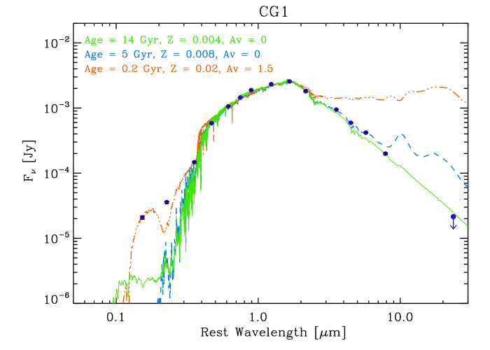
Figure 6: The observed SED of GC1 (from Galex FUV to Spitzer/MIPS 24 $\mu$m) (blue points) along with SSP models that best fit the SED (solid lines). None of the SSPs can fit the entire range of SEDs — the SSP that fits the UV data (red line) over-produces MIR flux, the SSP that fits the MIR data (green line) under-produces UV flux. Use of only the optical and NIR parts of the SED results in age-metallicity degeneracy (compare the values for the green and blue lines). The parameters of the models used in these fits do not produce the blue horizontal branch stars, which are known to be responsible for the UV emission in Galactic GCs.

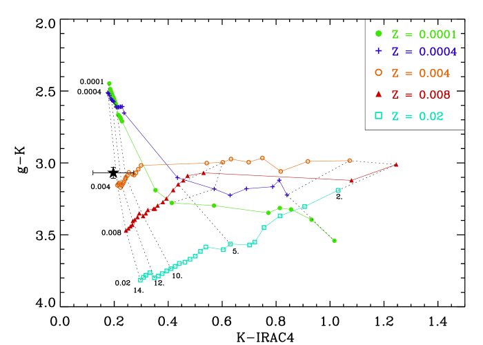
Figure 7: Colour-colour diagram formed using SDSS $g$, 2MASS $K$ and Spitzer 8.0$\mu$m bands. SSPs are shown for five values of metallicities ranging from Z=0.0001 to Z=0.02, and various ages between 2–14 Gyr. Dotted (almost vertical) lines join different metallicity points at fixed ages. The observed colours (shown by the asterisk) clearly indicate ages $>12$ Gyr, and $Z\la 0.004$.

In Figure 6 we show the results of this analysis. The points (blue) correspond to the galactic extinction-corrected data, while different lines represent different possible solutions that we have in our library. The first thing to note is that none of our SSP models can simultaneously fit the UV and the MIR part of the spectrum. Only very young (age$\la 200$ Myr), high metallicity ($Z\ga 0.2$), and highly reddened ($A_{V}\ga 1.5$ mag) models can reproduce the UV data (dash-dotted line). However, the reddening corresponding to $A_{V}=1.5$ mag in these models produces an emission at IR wavelengths very much in excess of the MIR data. Notice that the SSP shown in Figure 6 doesn’t include the reprocessed light corresponding to the absorption of $A_{V}\ga 1.5$ mag, inclusion of which will further widen the gap between this model and the observed SED at MIR wavelengths. If UV data are not considered in the analysis, the best fit corresponds to an old (formal age$=14$ Gyr), relatively metal-poor ($Z=0.004$) and dust-free ($A_{V}=0.0$ mag) SSP model (green solid line). For the sake of completeness, if we restrict the SED to fit only the optical to NIR bands, apart from the above solution, equally good fits are obtained for a younger (age$=5$ Gyr), but slightly metal-rich ($Z=0.008$) SSP with no reddening required, clearly illustrating the effect of the degeneracy between age and metallicity (blue dashed line). However, even in this case, the model produces an excess emission in the MIR part of the spectrum due to the dusty circumstellar envelopes around AGB stars, where the typical silicates’ emission feature clearly appears at $\sim 10~{}\mu$m. The analysis of SSP models that account for dusty circumstellar envelopes show that this feature gets stronger at increasing metallicity (and/or at intermediate ages), due to the correspondingly higher dust-mass-loss rate of the SSPs. On the other hand, the feature vanishes at very low metallicity and/or at very old ages. Therefore, the use of the MIR data and, more importantly, the upper limit at 24$\mu$m, rules out an age as young as 5 Gyr, and favours old ages and close to zero internal extinction. It is the combined optical to MIR analysis what ultimately breaks the age-metallicity degeneration and favours very old ($>$ 13 Gyr) and moderately metal-poor (Z$\lesssim$ 0.004) SSP models. This result is further illustrated in the $g-K$ vs $K-[8.0]$ diagram (Figure 7), where the observed colours of GC1 (shown by the asterisk) indicate an age $>12$ Gyr and metallicity $Z\lesssim 0.004$.

However, none of the above models fit the GALEX (and the SDSS-$u$) fluxes. The SSP flux in the UV is more than an order of magnitude lower than the observed GALEX fluxes, establishing clearly the presence of UV excess. This UV excess is an already known issue in massive GCs(e.g. Vink et al., 1999; D’Cruz et al., 2000; Brown et al., 2001; Busso et al., 2007). Blue horizontal branch stars (BHBs) are established to be the main reason for the UV excess in GCs. In canonical models of population synthesis for GCs (e.g. Lee et al., 1994), BHBs naturally appear in old, very metal-poor systems, whereas metal-rich systems have only red clump stars. GC1 is not metal-poor, and hence we expect only the red clump, and no UV excess, especially using the recently downward revised calibration of the mass-loss rates during the Red Giant Branch (Miglio et al., 2012). However, this problem is not unique to GC1 — many massive, relatively metal-rich galactic GCs are found to have hot BHBs (Rich et al., 1997). Lee et al. (1994) found these hot BHBs to contain an enhanced amount of helium. A second stellar generation with almost equal metallicity, but He-enriched, is nowadays the most likely explanation for the presence of the hot horizontal branch in galactic GCs (e.g. Caloi & D’Antona, 2007).

In order to check the possibility that the UV excess could be explained by accounting for the presence of a He-rich stellar population, we calculated a new set of SSP models for an enhanced value of initial He content. In more detail, we use PARSEC code to compute models for the same metallicity of the fit ($Z=0.004$), ages between 9 to 14 Gyr, and an initial He content equal to $Y=0.4$, a value that produces entire range of observed $T_{\rm eff}<30000$ K for the HB stars (Busso et al., 2007). It is worth noting that these models are fully consistent with the ones computed previously by adopting the canonical value of $Y=0.25$, as far as both the physical inputs and numerical assumptions are concerned. We re-did the fit, now accounting for data from FUV to IRAC4 bands, and where $F_{\rm mod}$ is a combination of the two sets of SSPs (one with the canonical Y value, and the other with $Y=0.4$), using $F_{\rm mod}=(1-f)\times F_{\rm mod,Y=0.25}+f\times F_{\rm mod,Y=0.4}$, where $f$ is the fraction of the He-rich population needed to fit the total SED.

In Figure 8, we show the comparison between the observational data (blue points), the best fit (red solid line, and red squares), and the previous best fit corresponding to the canonical He abundance (green thin solid line). As already discussed, the models computed by assuming a canonical He content ($Y=0.25$) are not able to reproduce the UV excess. By contrast, the presence of two stellar populations with similar ages and metallicities, but markedly distinct initial He content, reproduce the entire SED of GC1. The main population corresponding again to an age of $\sim$14.0 Gyr, a metallicity of $Z=0.004$ and the population with canonical He content contributes around 60% to the bolometric luminosity, while the He rich population corresponding to an SSP of 13.2 Gyr and a metallicity of $Z=0.004$, contributes 40% ($f=0.40$) to the total luminosity. This result is in agreement with the results by Caloi & D’Antona (2007) and Busso et al. (2007). They found that significant fractions, ranging between 35–60% of a He-rich stellar population, are needed in order to explain the morphology and the observational features of the HBs of NGC 6441 and NGC 6388. Moreover, by comparing the best models with and without a He-rich population (red vs. green lines in Fig. 8), one can see that the impact of the inclusion of the He-rich population is almost negligible at wavelengths longer than the $U$-band (see also Girardi et al., 2007).

The SED-inferred metallicity of $Z=0.004$ is in good agreement with that inferred from our analysis of Lick indices ($Z=0.0043$; see §4.1), putting GC1 clearly among the high metallicity GCs. The-SED inferred age ($\gtrsim 13$ Gyr) and the presence of second generation of bluer stars are also in good agreement with the star formation history inferred using STARLIGHT.

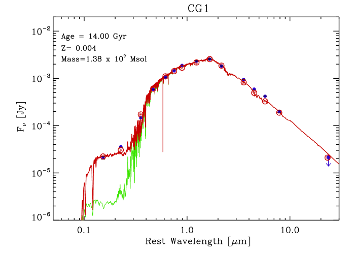
Figure 8: The observed SED of GC1 (from Galex FUV to Spitzer/MIPS 24 $\mu$m) (blue points) along with the multiple stellar generation model including the He-rich population with BHB stars, that best fits the entire SED (red solid line; 14 Gyr, $Z=0.004$, Y=0.40, $A_{V}=0.0$ mag). Green line is the standard model with a single stellar generation without the BHB stars (see text for more details).

Our analysis indicates that the inferred initial mass of GC1 is about $1.5\times 10^{7}$ M_⊙, 40% of which are enriched in He content. The inferred number of He-rich BHB stars (T${}_{\rm eff}>7000$ K) is $\sim 2523$ which produce a bolometric luminosity of about $2.524\times 10^{5}~{}\rm L_{\odot}$. Whitney et al. (1994) detected 1957 FUV bright sources in the massive galactic cluster $\omega$ Centauri, of which over 30% are extreme HB stars or hot post-AGB stars (D’Cruz et al., 2000). Busso et al. (2007), using the star counting technique, found 146 and 218 BHB stars in NGC 6441 and NGC 6388, respectively, two massive ($\sim 10^{6}$ M_⊙), old ($\sim 11$–13 Gyr) and metal-rich ($[Fe/H]\thickapprox-0.5$) bulge globular clusters. Ma et al. (2009) used the broad-band (FUV to NIR) SED fitting technique in G1 in M31, and found also a UV excess which would correspond to $\sim 165~{}\rm L_{\odot}$ FUV-bright, hot, extreme HB stars, which is more than 3 order of magnitude lower than the results we got for GC1, even though M31-G1 has a similar mass as GC1. However, we note that M31-G1 is metal-poor by more than a factor of 2 as compared to GC1. On the other hand, note that GC1, NGC 6441, NGC 6388 and even $\omega$ Centauri are massive and metal-rich globular clusters ($Z\gtrsim 0.004$), and only a He-rich old stellar population could give a significantly higher number of hot, evolved HB stars, as compared to the He-poor counterparts of the same age and lower metallicity (e.g. Lee et al., 1990, 2001; Yi et al., 1999; Caloi & D’Antona, 2007; Busso et al., 2007). The presence of He-rich stellar populations have also been proposed by Kaviraj et al. (2007b) to explain the UV emission of UV-bright clusters in M87. As far as the authors know, GC1 could be the cluster with the largest number of He-rich BHB stars.

We would like to point out, and it is easy to see in Fig. 8, that the best fit (red solid line) model under-produces emission at the NUV with respect to the observed data, most likely indicating that the BHB stars in our models are too hot. It is well established that the bluest HB stars are cooler at lower He enhancement values (e.g. Raimondo et al., 2002; D’Antona et al., 2005; Moehler et al., 2006; Caloi & D’Antona, 2007; Busso et al., 2007). Thus, it is likely that the He enhancement in GC1 is not as high as $Y=0.4$, but $\sim 0.35$. Determining the exact value of $Y$ is beyond the scope of this work, as it also depends on the mass-loss efficiency during the red giant evolution.

The presence of He-enriched stellar population would imply that GC1 must have had at least two episodes of star formation with the second generation of stars polluted by material ejected from the first generation of stars. The stars responsible for the pollution could be type II supernovae, rotating massive stars or massive-AGB stars (e.g. D’Antona et al., 2002; Renzini, 2008). The nature of the progenitor and how the ejected material can remain inside the potential well will be discussed in §5.

Given that the presence of a small fraction of He-enriched stars can give rise to an UV excess, it is not advisable to use UV fluxes while fitting SEDs to obtain age and metallicity of old simple populations. Ignoring the He-enriched stars in clusters with intrinsic UV excess would lead to overestimates of ages such as found in Kaviraj et al. (2007a) and Ma et al. (2009).

5 DISCUSSION AND CONCLUSIONS

5.1 Photometric mass

The derived photometric mass of $1.5\times 10^{7}$ $M_{\odot}$ corresponds to the mass at birth of the cluster using the Salpeter IMF (see §4.3). At the present age of $\sim 13.5$ Gyr, the cluster still contains 65% of the initial mass (51% in living stars, and 14% in stellar remnants). Thus, the present mass of the cluster with the Salpeter IMF is $1.0\times 10^{7}$ $M_{\odot}$. With the Kroupa (2001) IMF, the present mass would be $6.3\times 10^{6}$ $M_{\odot}$. The derived mass is comparable to the photometric mass of M31-G1 (see Table 1), whereas it is $\sim 4$ times more than that of $\omega$ Cen, the brightest GC in the Milky Way. In this section, we analyse whether this cluster shares properties that are established to be characteristics of massive GCs, and address the issue of its origin.

5.2 Dynamical state

The relatively high concentration index of $c=\log(r_{t}/r_{c})\sim 1.88$ suggests that the cluster is in a post-core collapse stage, where binaries at the centre of the cluster provide a source of energy to halt the collapse. The GC1 is expected to harbour a number of close low-mass binaries, which are expected to emit X-rays. The brightest GCs in galaxies are known to be X-ray emitters (e.g. Kundu & Whitmore (2002) in NGC 4472; Fabbiano et al. (2010) in NGC 4278), where the low-mass X-ray binaries are responsible for the X-ray emission. The X-ray missions ROSAT and Chandra, both have detected X-ray emission from GC1 (Immler & Wang, 2001; Swartz et al., 2003), with the latter reporting an X-ray luminosity of $5.1\pm 1.1\times 10^{37}$erg s^-1. The observed luminosity of GC1 corresponds to a system of a binary where the donor is an evolved giant star (Revnivtsev et al., 2011).

The cluster is at a projected distance of only 3.0 kpc from the nucleus of the galaxy. We now calculate the expected tidal radius of GC1, using the relation given by Spitzer (1987):
$R_{\rm t}=\left({M_{\rm C}\over{2M_{\rm G}}}\right)^{1/3}R_{\rm G}$,
where $R_{\rm G}=3.0$ kpc is the galactocentric radius of GC1, $M_{\rm C}=1.5\times 10^{7}$ $M_{\odot}$ is the mass of GC1, and $M_{\rm G}$ is the mass of the parent galaxy within the radius $R_{\rm G}$. Nantais & Huchra (2010) estimate a mass of $0.88\times 10^{11}$ $M_{\odot}$ within a galactocentric radius of 3.82 kpc. Substituting these values, we get a tidal radius of 116 pc. The observed $r_{t}=93$ pc in the $F814$-band is 80% of this value. Thus, the dynamical evolution of GC1 is not being affected by the tidal forces of the parent galaxy, unless the cluster is in a highly eccentric orbit and that it had a peri-centre radius as small as 2.0 kpc. The fact that the observed radial velocity of GC1 is consistent with that expected at the present radius, possibly rules out the object being in a highly eccentric orbit.

In a recent work, Gieles et al. (2011) divided the Galactic GCs into two categories — the expansion-dominated and evaporation-dominated. GCs in the first category are massive ones that are evolving without the tidal effects of the parent galaxy, resulting in the increase of their half-mass radius with time. The GCs in the second category are tidally limited, resulting in evaporation, and subsequent contraction. The observed mass of GC1 clearly puts it in the first category. If we extrapolate the $r_{\rm h}$-Mass relation that Gieles et al. (2011) obtained for the Galactic GCs to the mass of GC1, we obtain an $r_{\rm h}=1.26$ pc, which is around 4 times smaller as compared to the observed value. Thus, GC1 is in the expansion-dominated phase.

5.3 Metallicity and $\alpha$-enrichment

Colour distribution of GCs shows bimodality, which is principally due to a metallicity difference between two old populations (Brodie & Strader, 2006), with the metal-poor ($[Fe/H]<-1$) GCs being relatively bluer than their metal-rich counterparts. GC1 is metal-rich $[Fe/H]=-0.60\pm 0.10$, and moderately $\alpha$-enriched ([$\alpha/{\rm Fe}]\sim 0.2\pm 0.05$). Star formation episodes extending for more than $\gtrsim 1$ Gyr are not expected to show $\alpha$ enrichment, and hence the observed value of [$\alpha/{\rm Fe}$] rules out extended period of star formation. Thus, star formation and metal enrichment in this cluster should have happened over this short time-scale. This implies that the cluster was efficient in retaining all or most of metals ejected in the initial burst. Metals are expelled from stars in the form of high velocity winds of high mass stars, through explosion of SNII, and through the winds of AGB stars. With the inferred photometric mass of $1.0\times 10^{7}$ $M_{\odot}$, and a concentration parameter of $\sim 1.88$, we estimate an escape velocity at the tidal radius of 146 km s^-1 at present, using the expression given by Georgiev et al. (2009). Given that the initial cluster mass is expected to be higher, and the $r_{h}$ lower than the presently observed values, the escape velocities during the first gigayear of star formation would have been higher than this value. Terminal velocity of winds in AGBs of stars of metallicities $[Fe/H]=-0.60$ is expected to be around 50 km s^-1, whereas the velocity of winds from high-mass stars, and supernova ejecta would be much higher than the escape velocities. However, the cluster potential was deep enough to trap metals from AGB winds, resulting in enrichment of the interstellar medium before the star formation ceased. The potential well, however, was not deep enough to trap all the metals generated in the cluster.

Trapping of metal-enriched gas also leads to the formation of helium enriched second generation of stars, that at present show up as blue HB stars. The SED of the cluster, especially the flux in the Galex bands, clearly suggests an extended blue HB, consisting of $\sim 2500$ stars.

5.4 Is GC1 the nucleus of a dissolved dwarf galaxy?

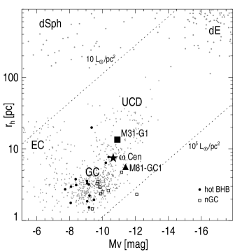
Figure 9: The location of GC1 in the size-luminosity plane compared to for various kinds of spherodal systems (dSph: dwarf spherodals, dE: dwarf ellipticals, UCD: ultra compact dwarfs, EC: extended or fuzzy clusters, nGC: nuclei of dwarf galaxies, E-BHB: Galactic GCs with extended BHB). Data for galactic and extragalactic GCs are denoted by GC. The two well-known massive clusters, $\omega$ Cen and M31-G1 are identified. The lines of constant mean surface brightness of $10^{5}$ and 10 L☉/pc² are shown by the two diagonal lines. During stripping of dwarf galaxies, their nuclei would fade and expand, resulting in decrease of their surface brightness. Like $\omega$ Cen and M31-G1, a high surface brightness nGC could be the progenitor of GC1.

GC1 is clearly one of the most massive clusters in the local Universe. Ever since the success of the numerical simulations of Bekki & Freeman (2003) in explaining the observed properties of $\omega$ Cen, massive GCs are often considered as nuclei of stripped dwarf galaxies. We here discuss whether GC1 also fits into this picture. Kormendy’s classical work (Kormendy, 1985) led to the use of observational planes formed from two or more of the following four quantities — central or mean surface brightness, core or half-light radius, total absolute magnitude and central velocity dispersions — to address the inter-relation between different spheroidal systems (e.g. Boselli et al., 2008; van den Bergh, 2010; Taylor et al., 2010).

Georgiev et al. (2009) used the $r_{\rm h}$ vs $M_{v}$ diagram to address the origin of GCs that have hot BHBs. More recently, Brodie et al. (2011) and Forbes et al. (2013) have used this diagram to illustrate the continuity of properties of different spheroidal systems. In Figure 9, we show the $r_{\rm h}$ vs $M_{v}$ diagram, where data for GC1 are plotted along with those for other spheroidal systems. Data for galactic and extragalactic GCs, extended clusters (EC; also known as Fuzzy Clusters), UCDs and cores of dwarf spheroidals (dSph) and dwarf ellipticals (dE) are taken from Brodie et al. (2011). Data for nucleated dwarf galaxies (nGC; also known as nuclear GCs), and galactic GCs that have hot BHBs from Georgiev et al. (2009). Data for M31-G1 and $\omega$ Cen were taken from the sources listed in Table 1. The diagonal lines show the locus of constant mean surface density of $10^{5}$ and 10 L☉/pc², within the half-light radius. During stripping of a dwarf galaxy, its nucleus is expected to experience expansion and also fade in intensity (Bekki & Freeman, 2003). This would reduce the surface brightness, moving the points roughly along a direction perpendicular to the constant surface brightness lines.

With a mean surface density of $1.5\times 10^{4}$ L☉/pc², GC1 is among the highest surface density objects, especially among the luminous objects. The classes of objects that are more massive than GC1 are cores of dEs, UCDs and nGCs. The progenitor candidate should have higher surface density than the presently observed value for GC1 to account for the expansion and fading associated with stripping. The high surface brightness nucleated dwarf galaxies are the only objects satisfying this criterion, and hence are the most likely progenitors of GC1. It is interesting to note that the observed ellipticity of GC1 ($\epsilon=0.12$), is almost identical to the mean ellipticity of nuclei of dwarf galaxies ($<\epsilon>=0.11$; Georgiev et al. (2009)). Georgiev et al. (2009) propose nuclei of dwarf galaxies as progenitors of GCs with hot BHBs, a property shared by GC1. Thus, all the observed evidence points towards a dwarf galaxy nuclear origin for GC1.

It is most likely that the nucleated dwarf galaxy that was once upon a time the progenitor of GC1 was intact for at least the first 1 Gyr, helping in its metal-enrichment. Subsequently, as the dwarf galaxy started accreting onto M81, the tidal forces dissolved the galaxy, leaving behind the compact nucleus indistinguishable in appearance from a classical GC.

6 Summary

We investigate the nature of the brightest GC in M81 by carrying out a detailed analysis of multi-band photometric and optical spectroscopic data. We establish that the cluster is old (age$\ga 13$ Gyr) and metal-rich ($[Fe/H]=-0.60\pm 0.10$). The UV excess suggests the presence of $\sim 2500$ hot blue horizontal branch stars, a characteristic common in many metal-rich GCs. The cluster is bluer in its core, suggesting that the hot BHB stars are concentrated at the centre of the cluster. The radial profile of the cluster can be fitted very well with a King profile of a core radius $r_{c}=1.2$ pc, and a logarithmic concentration index of 1.88. The low $r_{c}$ and high concentration index suggest that the cluster is in a post core-collapse phase. All the observed properties of GC1 support the idea that it could be the left-over nucleus of a dwarf galaxy that has been dissolved during its accretion onto M81 in the early epoch of its formation.

7 ACKNOWLEDGMENTS

We would like to thank the Hubble Heritage Team at the Space Telescope Science Institute for making the M81 images publicly available. We also thank the anonymous referee for many useful comments that have led to an improvement of the original manuscript. This work is partly supported by CONACyT (Mexico) research grants CB-2010- 01-155142-G3 (PI:YDM), CB-2011-01-167281-F3 (PI:DRG) and CB-2012-183013 (PI:OV).

References

- Alongi et al. (1993) Alongi M., Bertelli G., Bressan A., Chiosi C., Fagotto F., Greggio L., Nasi E., 1993, A&AS, 97, 851
- Annibali et al. (2007) Annibali, F., Bressan, A., Rampazzo, R., Zeilinger, W. W., & Danese, L. 2007, A&A, 463, 455
- Asplund et al. (2009) Asplund M., Grevesse N., Sauval A. J., Scott P., 2009, ARA&A, 47, 481
- Bekki & Freeman (2003) Bekki, K., & Freeman, K. C. 2003, MNRAS, 346, L11
- Bertin & Arnouts (1996) Bertin E., Arnouts S., 1996, A&AS, 117, 393
- Bianchi et al. (2005) Bianchi, L., Thilker, D. A., Burgarella, D., et al. 2005, ApJL, 619, L71
- Le Borgne et al. (2003) Le Borgne et al. 2003, A&A, 402, 433
- Boselli et al. (2008) Boselli, A., Boissier, S., Cortese, L., & Gavazzi, G. 2008, ApJ, 674, 742
- Bregman et al. (1998) Bregman, J. N., Athey, A. E., Bregman, J. D., & Temi, P. 1998, Bulletin of the American Astronomical Society, 30, 1261
- Bressan et al. (1993) Bressan A., Fagotto F., Bertelli G., Chiosi C., 1993, A&AS, 100, 647
- Bressan et al. (1998) Bressan, A., Granato, G. L., & Silva, L. 1998, A&A, 332, 135
- Bressan et al. (2001) Bressan, A., Aussel,H., Granato, G. L., et al. 2001, Astrophysics and Space Science Supplement, 277, 251
- Bressan et al. (2006) Bressan, A., Panuzzo, P., Buson, L., et al. 2006, ApJL, 639, L55
- Bressan et al. (2012) Bressan, A., Marigo, P., Girardi, L., et al. 2012, MNRAS, 427, 127
- Bridžius et al. (2008) Bridžius, A., Narbutis, D., Stonkutė, R., Deveikis, V., & Vansevičius, V. 2008, Baltic Astronomy, 17, 337
- Brodie & Huchra (1990) Brodie, J. P., & Huchra, J. P. 1990, ApJ, 362, 503
- Brodie & Strader (2006) Brodie J. P., Strader J., 2006, ARA&A, 44, 193
- Brodie et al. (2011) Brodie J. P., Romanowsky A. J., Strader J., Forbes D. A., 2011, AJ, 142, 199
- Brouillet, Combes, & Baudry (1991) Brouillet N., Combes F., Baudry A., 1991, IAUS, 146, 347
- Brown et al. (2001) Brown, T. M., Sweigart, A. V., Lanz, T., Landsman, W. B., & Hubeny, I. 2001, ApJ, 562, 368
- Bruzual & Charlot (2003) Bruzual G., Charlot S., 2003, MNRAS, 344, 1000
- Busso et al. (2007) Busso, G., Cassisi, S., Piotto, G., et al. 2007, A&A, 474, 105
- Caloi & D’Antona (2007) Caloi, V., & D’Antona, F. 2007, A&A, 463, 949
- Cardelli et al. (1989) Cardelli J. A., Clayton G. C., Mathis J. S., 1989, ApJ, 345, 245
- Cid Fernandes et al. (2005) Cid Fernandes R., Mateus A., Sodr’e L., Stasi´nska G., Gomes J. M., 2005, MNRAS, 358, 363
- Chabrier (2001) Chabrier, G. 2001, ApJ, 554, 1274
- Chabrier (2003) Chabrier G., 2003, PASP, 115, 763
- D’Antona et al. (2002) D’Antona, F., Caloi, V., Montalbán, J., Ventura, P., & Gratton, R. 2002, A&A, 395, 69
- D’Antona et al. (2005) D’Antona, F., Bellazzini, M., Caloi, V., et al. 2005, ApJ, 631, 868
- D’Cruz et al. (2000) D’Cruz, N. L., O’Connell, R. W., Rood, R. T., et al. 2000, ApJ, 530, 352
- Fabbiano et al. (2010) Fabbiano, G., Brassington, N. J., Lentati, L., et al. 2010, ApJ, 725, 1824
- Fagotto et al. (1994a) Fagotto F., Bressan A., Bertelli G., Chiosi C., 1994a, A&AS, 104, 365
- Fagotto et al. (1994b) Fagotto F., Bressan A., Bertelli G., Chiosi C., 1994b, A&AS, 105, 29
- Fitzpatrick (1999) Fitzpatrick, E. L. 1999, PASP, 111, 63
- Forbes et al. (2013) Forbes D., Pota V., Usher C., Strader J., Romanowsky A., Brodie J., Arnold J., Spitler L., 2013, arXiv, arXiv:1306.5245
- Freedman et al. (1994) Freedman W. L., et al., 1994, ApJ, 427, 628
- Georgiev et al. (2009) Georgiev, I. Y., Puzia, T. H., Hilker, M., & Goudfrooij, P. 2009, MNRAS, 392, 879
- Gieles et al. (2011) Gieles, M., Heggie, D. C., & Zhao, H. 2011, MNRAS, 413, 2509
- Girardi et al. (1996) Girardi, L., Bressan, A., Chiosi, C., Bertelli, G., & Nasi, E. 1996, A&AS, 117, 113
- Girardi et al. (2002) Girardi L., Bertelli G., Bressan A., Chiosi C., Groenewegen M. A. T., Marigo P., Salasnich B., Weiss A., 2002, A&A, 391, 195
- Girardi et al. (2007) Girardi, L., Castelli, F., Bertelli, G., & Nasi, E. 2007, A&A, 468, 657
- Goudfrooij et al. (2001) Goudfrooij P., Mack J., Kissler-Patig M., Meylan G., Minniti D., 2001, MNRAS, 322, 643
- Haşegan et al. (2005) Haşegan, M., Jordán, A., Côté, P., et al. 2005, ApJ, 627, 203
- Harris (1996) Harris W. E., 1996, AJ, 112, 1487
- Immler & Wang (2001) Immler, S., & Wang, Q. D. 2001, ApJ, 554, 202
- Jang et al. (2012) Jang I. S., Lim S., Park H. S., Lee M. G., 2012, ApJ, 751, L19
- Kaviraj et al. (2007a) Kaviraj, S., Sohn, S. T., O’Connell, R. W., et al. 2007a, MNRAS, 377, 987
- Kaviraj et al. (2007b) Kaviraj, S., Rey, S.-C., Rich, R. M., Yoon, S.-J., & Yi, S. K. 2007b, MNRAS, 381, L74
- Kennicutt et al. (2003) Kennicutt, R. C., Jr., Armus, L., Bendo, G., et al. 2003, PASP, 115, 928
- King (1962) King I., 1962, AJ, 67, 471
- King (1966) King I. R., 1966, AJ, 71, 64
- Konstantopoulos et al. (2009) Konstantopoulos, I. S., Bastian, N., Smith, L. J., Westmoquette, M. S., Trancho, G., & Gallagher, J. S. 2009, ApJ, 701, 1015
- Kormendy (1985) Kormendy J., 1985, ApJ, 295, 73
- Kroupa (2001) Kroupa P., 2001, MNRAS, 322, 231
- Kundu & Whitmore (2002) Kundu, A., & Whitmore, B. 2002, Extragalactic Star Clusters, 207, 229
- Larsen (1999) Larsen S. S., 1999, A&AS, 139, 393
- Lee et al. (1990) Lee, Y.-W., Demarque, P., & Zinn, R. 1990, ApJ, 350, 155
- Lee et al. (1994) Lee, Y.-W., Demarque, P., & Zinn, R. 1994, ApJ, 423, 248
- Lee et al. (2001) Lee, Y.-W., Yoon, S.-J., Rey, S.-C., & Chaboyer, B. 2001, Astrophysical Ages and Times Scales, 245, 343
- Ma et al. (2009) Ma J., et al., 2009, RAA, 9, 641
- Mateus et al. (2006) Mateus A., Sodr’e L., Cid Fernandes R., Stasi´nska G., SchoenellW., Gomes J. M., 2006, MNRAS, 370, 721
- Mayya et al. (2008) Mayya, Y. D., Romano R., Rodríguez-Merino L. H., Luna A., Carrasco L., & Rosa-González D. 2008, ApJ, 679, 404
- McLaughlin & van der Marel (2005) McLaughlin D. E., van der Marel R. P., 2005, ApJS, 161, 304
- Meylan et al. (1995) Meylan, G., Mayor, M., Duquennoy, A., & Dubath, P. 1995, A&A, 303, 761
- Meylan et al. (2001) Meylan G., Sarajedini A., Jablonka P., Djorgovski S. G., Bridges T., Rich R. M., 2001, AJ, 122, 830
- Mieske et al. (2006) Mieske, S., Jordán, A., Côté, P., et al. 2006, ApJ, 653, 193
- Miglio et al. (2012) Miglio, A., Brogaard, K., Stello, D., et al. 2012, MNRAS, 419, 2077
- Moehler et al. (2006) Moehler, S., & Sweigart, A. V. 2006, A&A, 455, 943
- Nantais & Huchra (2010) Nantais J. B., Huchra J. P., 2010, AJ, 139, 2620
- Perelmuter & Racine (1995) Perelmuter J.-M., Racine R., 1995, AJ, 109, 1055
- Pérez-González et al. (2006) Pérez-González P. G., et al., 2006, ApJ, 648, 987
- Phillipps et al. (2001) Phillipps, S., Drinkwater, M. J., Gregg, M. D., & Jones, J. B. 2001, ApJ, 560, 201
- Raimondo et al. (2002) Raimondo, G., Castellani, V., Cassisi, S., Brocato, E., & Piotto, G. 2002, ApJ, 569, 975
- Renzini (2008) Renzini, A. 2008, MNRAS, 391, 354
- Revnivtsev et al. (2011) Revnivtsev, M., Postnov, K., Kuranov, A., & Ritter, H. 2011, A&A, 526, A94
- Rich et al. (1997) Rich, R. M., Sosin, C., Djorgovski, S. G., et al. 1997, ApJL, 484, L25
- Rodríguez-Merino et al. (2011) Rodríguez-Merino, L. H., Rosa-González, D.,& Mayya, Y. D. 2011, ApJ, 726, 51
- Salpeter (1955) Salpeter E. E., 1955, ApJ, 121, 161
- Sánchez-Blázquez P. et al. (2006) Sánchez-Blázquez P. et al., 2006, MNRAS, 371, 703
- Santiago-Cortés, Mayya, & Rosa-González (2010) Santiago-Cortés M., Mayya Y. D., Rosa-González D., 2010, MNRAS, 405, 1293
- Schiavon et al. (2005) Schiavon, R. P., Rose, J. A.,Courteau, S., & MacArthur, L. A. 2005, ApJS, 160, 163
- Schlafly & Finkbeiner (2011) Schlafly, E. F., & Finkbeiner, D. P. 2011, ApJ, 737, 103
- Schlegel (1998) Schlegel D. J., Finkbeiner D. P., Davis M., 1998, ApJ, 500, 525
- Spitzer (1987) Spitzer, L. 1987, Princeton, NJ, Princeton University Press, 1987, p15
- Strader et al. (2005) Strader J., Brodie J. P., Cenarro A. J., Beasley M. A., Forbes D. A., 2005, AJ, 130, 1315
- Swartz et al. (2003) Swartz, D. A., Ghosh, K. K., McCollough, M. L., et al. 2003, ApJS, 144, 213
- Taylor et al. (2010) Taylor, M. A., Puzia, T. H., Harris, G. L., et al. 2010, ApJ, 712, 1191
- Thomas et al. (2003) Thomas, D., Maraston,C., & Bender, R. 2003, MNRAS, 339, 897
- Trager et al. (1998) Trager, S. C., Worthey,G., Faber, S. M., Burstein, D., & Gonzalez, J. J. 1998, ApJS, 116, 1
- van den Bergh (2010) van den Bergh S., 2010, AJ, 140, 1043
- Vink et al. (1999) Vink, J. S., Heap, S. R., Sweigart, A. V., Lanz, T., & Hubeny, I. 1999, A&A, 345, 109
- Whitmore & Schweizer (1995) Whitmore B. C., Schweizer F., 1995, AJ, 109, 960
- Whitney et al. (1994) Whitney, J. H., O’Connell, R. W., Rood, R. T., et al. 1994, AJ, 108, 1350
- Worthey et al. (1994) Worthey, G., Faber, S. M., Gonzalez, J. J., & Burstein, D. 1994, ApJS, 94, 687
- Yi et al. (1999) Yi, S., Lee, Y.-W., Woo, J.-H., et al. 1999, ApJ, 513, 128
- Zinnecker et al. (1988) Zinnecker, H., Keable, C. J., Dunlop, J. S., Cannon, R. D., & Griffiths, W. K. 1988, The Harlow-Shapley Symposium on Globular Cluster Systems in Galaxies, 126, 603