Bayesian Degree-Corrected Stochastic Blockmodels for Community Detection

Abstract

Community detection in networks has drawn much attention in diverse fields, especially social sciences. Given its significance, there has been a large body of literature with approaches from many fields. Here we present a statistical framework that is representative, extensible, and that yields an estimator with good properties. Our proposed approach considers a stochastic blockmodel based on a logistic regression formulation with node correction terms. We follow a Bayesian approach that explicitly captures the community behavior via prior specification. We further adopt a data augmentation strategy with latent Pólya-Gamma variables to obtain posterior samples. We conduct inference based on a principled, canonically mapped centroid estimator that formally addresses label non-identifiability and captures representative community assignments. We demonstrate the proposed model and estimation on real-world as well as simulated benchmark networks and show that the proposed model and estimator are more flexible, representative, and yield smaller error rates when compared to the MAP estimator from classical degree-corrected stochastic blockmodels.

and t2Supported by NSF grant DMS-1107067.

1 Introduction

Networks can be used to describe interactions among objects in diverse fields such as physics (Newman, 2006), biology (Hancock et al., 2010), and especially social sciences (Zachary, 1977; Adamic and Glance, 2005). In network theory, objects are represented by nodes and their interactions by edges. Clusters of nodes that share many edges between them but that, in contrast, do not interact often with nodes in other clusters can be thought of as communities. This characterization follows a traditional approach in social sciences that aims at discerning the structure of a network according to relationship patterns among “actors”, e.g. friendship or collaboration. These interaction patterns may reflect “assortativity”, a concept that originated in the ecological and epidemiological literature (Albert and Barabási, 2002): it refers to the tendency of nodes to associate with other similar nodes in a network. Among measures of similarity, the degree of a node is of common interest in the study of assortativity in networks (Newman, 2002, 2003; Vázquez, 2003), that is, assortative networks usually show a preference for high-degree nodes to connect to other high-degree nodes. We expect in some applications that actors exercise assortativity and prefer to group themselves according to similarity or kinship in communities, and so communities are dense in within-group associations but sparse in between-group interactions. Thus, not surprisingly, community detection has sparked great interest in many fields where recent applications aim at characterizing the structure of a network by detecting its communities.

There have been many approaches to address community detection (see Section 2 for a more thorough review), but a common modeling choice is to treat actors as behaving similarly given their respective communities. This structural equivalence assumption is at the core of blockmodels (Lorrain and White, 1971), which were later extended to stochastic blockmodels (Holland and Leinhardt, 1981; Fienberg et al., 1985). Here, to tackle community detection, we adopt a hierarchical Bayesian stochastic blockmodel where group labels are random. We contend that a suitable prior specification is essential to accurately characterize assortative behavior, and thus that a Bayesian approach is essential to community detection (see, e.g., the examples in Section 7.1.) Our results can be connected to the work of Nowicki and Snijders (2001), Karrer and Newman (2011) and Hofman and Wiggins (2008) but we make two important distinctions: (i) we capture community behavior by explicitly requiring that the probability of within-group associations is higher than between-group relations; and (ii) we address parameter and label non-identifiability issues directly by remapping configurations to a unique canonical space. The first point is important in light of the examples in the last section. The second point allows us to sample from the posterior space of label configurations more efficiently and to formally define an estimator based on a meaningful loss function. Moreover, our model can be related to the work of Mariadassou et al. (2010) and Vu et al. (2013) as they are all based on exponential-family clustering frameworks, but our model is different from theirs in two respects besides the two points just mentioned: (i) we make exact inference by adopting latent variables, rather than adopting approximate variational approaches; and (ii) we add more flexibility by requiring hyper-prior structure on model parameters controlling degree correction.

More specifically, we make the following contributions:

1. We propose a Bayesian degree-corrected stochastic blockmodel for community detection that explicitly characterizes community behavior. We discuss this new model and how we account for parameter non-identifiability in Section 3.

2. We treat label non-identifiability issues by defining a canonical projection of the space of label configurations in Section 4.

3. We develop an efficient posterior sampler by identifying good initial configurations through approximate mode finding and then exploring a Gibbs sampler based on a data augmentation strategy in Section 5.

4. We propose a remapped centroid estimator for community inference in Section 6. This new estimator is based on Hamming loss and is arguably a good representative of a projected space of label configurations.

In Section 7 we show that our proposed method is efficient and able to fit medium-sized networks with thousands of nodes in reasonable time. Moreover, we show that our proposed estimator yields, in practice, smaller misclassification rates due to a more refined loss function when compared to the ML-based estimators. Finally, in Section 8, we offer some concluding remarks and directions for future work.

2 Prior and Related Work

There is a large body of literature in community detection, given its significance and interest. Traditional methods include graph partitioning (Kernighan and Lin, 1970; Barnes, 1982), hierarchical clustering (Hastie et al., 2001), and spectral clustering (Donath and Hoffman, 1973; Von Luxburg, 2007; Rohe et al., 2011); while these methods are heuristic and thus suitable for large networks, they do not address directly community detection but aim instead at partitioning the network according to edge densities between groups and thus identifying connection “bottlenecks”.

The concept of modularity better captures community structure by also taking within-group edge densities into account (Newman and Girvan, 2004; Newman, 2006). Optimization methods based on modularity can then be used to detect communities, but since modularity optimization is NP-complete (Brandes et al., 2007), interest lies mostly in approximated methods such as the greedy method of Newman (2004) and extremal optimization (Duch and Arenas, 2005; Bickel and Chen, 2009). However, there are still drawbacks: methods based on modularity may fail in detecting small communities and thus exhibit a “resolution limit” (Fortunato and Barthelemy, 2007). Latent space network models (Hoff et al., 2002), latent variable models (Hoff et al., 2005), and latent position cluster models (Handcock et al., 2007) assume that the probability of an interaction depends on node-specific latent factors such as the distance between two nodes in an unobserved continuous “social space”; these models are generalizations of exponential random graph models [ERGMs; see (Robins et al., 2007)] where community structure is assumed from cluster structure in the latent space.

There are many other methods to mention [see, for example, the review in (Parthasarathy et al., 2011)], but we focus on parametric statistical approaches where inference on community structure is based on an assumed model of association. The motivation is that since there are many possible community configurations, that is, assignment of actors to communities, we want to not only infer communities, but to also assess how likely each configuration is according to the model.

The first endeavors in such parametric models—albeit not in community detection—are the $p_{1}$ exponential family models due to Holland and Leinhardt (1981). These models follow a log-linear formulation (Fienberg and Wasserman, 1981) with parameters that are related to in- and out-degrees and edge densities. Later, these models were extended to incorporate actor and group parameters (Fienberg et al., 1985; Tallberg, 2005; Daudin et al., 2008). Wang and Wong (1987) further adapted the models to consider a block structure through stochastic blockmodels [SBMs (Holland et al., 1983; Anderson et al., 1992)], yielding $p_{1}$ blockmodels. Zanghi et al. (2010), Mariadassou et al. (2010) and Vu et al. (2013) proposed scalable approximate variational approaches based on modified version of those $p_{1}$ (block)models.

Stochastic blockmodels explore a simpler model structure where the probability of an association between two actors depends on the groups to which they belong, that is, two actors within the same group are stochastically equivalent. Karrer and Newman (2011) developed an SBM that allows for degree-correction, that is, models where the degree distribution of nodes within each group can be heterogeneous. Celisse et al. (2012), Choi et al. (2012) and Bickel et al. (2013) addressed the asymptotic inference in SBM by use of maximum likelihood and variational approaches. More flexible approaches generalize the SBM by adopting a hierarchical Bayesian setup that regards probabilities of association as random and group membership as latent variables (Snijders and Nowicki, 1997; Nowicki and Snijders, 2001; Hofman and Wiggins, 2008). As in all latent mixture models, label non-identifiability is a known problem since multiple label assignments yield the same partition into communities; ultimately, we only care if two actors are in the same community or in different communities. It is also possible to incorporate node attributes in the model (Kim and Leskovec, 2011; Fosdick and Hoff, 2013) and to allow actors to belong to more than one community (Airoldi et al., 2008).

3 A Bayesian Stochastic Blockmodel for Community Detection

Under our community detection setup we assume a fixed number of groups $K\geq 2$ and we are given, as data, a matrix $[A]_{ij}$ representing relationships between “actors” $i$ and $j$ in a network with $n>K$ nodes. We represent the assignment of actors to communities through $\sigma:\{1,\ldots,n\}\mapsto\{1,\ldots,K\}$, a vector of labels: $\sigma_{i}=k$ codes for the $i$-th individual belonging to the $k$-th community.

A simple stochastic blockmodel specifies that the probability of an edge between actors $i$ and $j$ depends only on their labels $\sigma_{i}$ and $\sigma_{j}$, and that $\sigma$ follows a product multinomial distribution:

$$A_{ij}{\,|\,}\mathbf{\sigma},\theta\stackrel{{\scriptstyle\text{\tiny ind}}}{{\sim}}\mbox{\sf Bern}\big{(}\theta_{\sigma_{i}\sigma_{j}}\big{)}, \qquad i,j=1,\ldots,n,i<j,$$ (1)

$$\sigma_{i}\stackrel{{\scriptstyle\text{\tiny iid}}}{{\sim}}\mbox{\sf MN}(1;\mathbf{\pi}), \qquad i=1,\ldots,n,$$

where $\mathbf{\pi}$ is a vector of prior probabilities over $K$ labels, parameter $\theta_{kk}$ is the “within” probability of a relationship in community $k$, and $\theta_{kl}$ is the “between” probability of a relationship for communities $k$ and $l$, $k,l=1,\ldots,K$, $k<l$. If we define $\theta_{w}\doteq\theta_{11}=\cdots=\theta_{KK}$ and $\theta_{b}\doteq\theta_{12}=\cdots=\theta_{K-1,K}$, we have a simpler model with single within and between probabilities (Hofman and Wiggins, 2008).

We regard SBMs as log-linear models and exploit this formulation to define a node-corrected SBM by

$$A_{ij}{\,|\,}\sigma,\gamma,\eta\stackrel{{\scriptstyle\text{\tiny ind}}}{{\sim}}\mbox{\sf Bern}\big{(}\text{logit}^{-1}(\gamma_{\sigma_{i}\sigma_{j}}+\eta_{i}+\eta_{j})\big{)}$$ (2)

where, in logit scale, parameters $\gamma$ capture within and between community probabilities of association and node intercepts $\eta=(\eta_{1},\dots,\eta_{n})$ capture the expected degrees of the nodes. To avoid redundancies, we only code $\gamma_{kl}$ for $k\leq l$. We note that without $\eta$, model (2) is equivalent to model (1) with $\gamma_{kl}=$logit$(\theta_{kl})$. We also remark that we call the above model node-corrected, which is arguably more suitable for a broader generalized linear model formulation; in Karrer and Newman’s approach the observed $A_{ij}$ follow a Poisson distribution, and so $\eta$ is related to expected log degrees, and hence their degree-correction denomination (Karrer and Newman, 2011).

3.1 Parameter Identifiability

In what follows, to simplify the notation we group $\beta=(\gamma,\eta)$ and define the design matrix $X$ associated to model (2) such that

$$A_{ij}{\,|\,}\sigma,\beta\stackrel{{\scriptstyle\text{\tiny iid}}}{{\sim}}\text{\sf Bern}\big{(}\text{logit}^{-1}(x_{ij}(\sigma)^{\top}\beta)\big{)}.$$

Note that we make explicit the dependence of each row $x_{ij}$ on the labels $\sigma$. Model (2) has then $\binom{K}{2}+K+n$ parameters, but the next result shows that only $\binom{K}{2}+n$ parameters are needed for the model to be identifiable if each community has at least two nodes (the proof is in Appendix 9.1.)

Theorem 1.

The design matrix $X$ associated with model (2) has the following properties:

1. It has $K$ linearly dependent columns.

2. It is full column-ranked if and only if each community has at least two nodes.

Based on these two criteria, to attain an identifiable model we remove $K$ parameters from $\gamma$ and modify the prior on $\sigma$ to a constrained multinomial distribution,

$${\mathbb{P}}(\sigma)\propto\prod_{k=1}^{K}I(N_{k}>1)\prod_{i=1}^{n}\pi_{k}^{I(\sigma_{i}=k)},$$

where $I(\cdot)$ is the indicator function and $N_{k}=\sum_{i}I(\sigma_{i}=k)$ is the number of nodes in community $k$. There are still problems with label identifiability that we address by label remapping in the Section 4; for now, to allow for a straightforward remapping of community labels, we just set

$$\gamma_{11}=\cdots=\gamma_{KK}=0$$ (3)

to remove the redundant $\gamma$ parameters.

3.2 Hierarchical model for community detection

We attain a more realistic model by further setting a hyper-prior distribution on $\gamma=(\gamma_{12},\ldots,$ $\gamma_{K-1,K})$, $\eta$, and $\pi$,

$$\beta=(\gamma,\eta) \sim I(\gamma\leq 0)\cdot N\Big{(}0,\tau^{2}I_{n+\binom{K}{2}}\Big{)},$$ (4)

$$\pi \sim\mbox{\sf Dir}(\alpha_{1},\dots,\alpha_{K}),$$

where $\tau^{2}$ controls how informative the prior is. The prior on $\gamma$ and $\eta$ can be seen as a ridge regularization for the logistic regression in (2). The constraint $\gamma\leq 0$ in this stochastic blockmodel is essential to community detection since we should expect as many as or fewer edges between communities than within communities on average, and thus that the log-odds of between and within probabilities is non-positive. The conjugate prior on $\pi$ adds more flexibility to the model, and is important when identifying communities of varied sizes and alleviating resolution limit issues.

4 Label Identifiability

Since the likelihood in (2) only considers if individuals are in the same community or not, labels are not identifiable due to this stochastic equivalence. Moreover, if $\pi$ follows a strongly informative symmetric Dirichlet, $\alpha=W\cdot 1_{K}$ with $W$ large, then the marginal prior on $\sigma$ is approximately non-identifiable:

$${\mathbb{P}}(\sigma)=\int{\mathbb{P}}(\sigma{\,|\,}\pi){\mathbb{P}}(\pi)\text{d}\pi=\frac{\prod_{k}\Gamma(N_{k}+W)/\Gamma(W)}{\Gamma(n+KW)/\Gamma(KW)}\approx\frac{\prod_{k}W^{N_{k}}}{(KW)^{n}}=\frac{1}{K^{n}}.$$

Since $\sigma_{i}$ are i.i.d. multinomial, then if $\pi$ is non-informative, $\mathbf{\pi}=(1/K,\ldots,$ $1/K)$, the labels are not identifiable in the posterior ${\mathbb{P}}(\sigma|A)$ either. In fact, non-identifiability issues occur within a group of labels $\mathcal{I}$ whenever $\pi_{i}=\pi_{j}$ for all $i,j\in\mathcal{I}$, but we discuss a non-informative $\pi$ for simplicity and because that is a common modeling choice.

A common approach in latent class models to fix label non-identifiability is to fix an arbitrary order in the parameters (Gelman et al., 2003, Chapter 18), e.g. $\gamma_{12}<\cdots<\gamma_{K-1,K}$. However, as Nowicki and Snijders (2001) point out, this solution can lead to imperfect identification of the classes if the parameters are close with high posterior probability; a major drawback then is that parameters and labels can be interpreted incorrectly. To address this problem, a label switching algorithm was proposed by Stephens (2000) in the context of MCMC sampling, but it is slow in practice. Another approach is to simply focus on permutation-invariant functions; in particular, when estimating $\sigma$, we can adopt a permutation-invariant loss, such as Binder’s loss (Binder, 1978). We discuss such approach in more detail in Section 6. Next, we propose an alternative, simpler procedure to remap labels and address non-identifiability.

4.1 Canonical Projection and Remapping Labels

Let $L\doteq\{1,\ldots,K\}$ and $\mathcal{L}=\{\sigma\in L^{n}:N_{k}(\sigma)>1,k=1,\ldots,K\}$ be the space of labels with positive prior probability. If $\rho$ is any permutation of the labels then ${\mathbb{P}}(\sigma|A)={\mathbb{P}}(\rho(\sigma)|A)$, where $(\rho(\sigma))_{j}=\rho(\sigma_{j})$ for $j=1,\ldots,n$. Non-identifiability here means that ${\mathbb{P}}(\cdot{\,|\,}A)$ is invariant under $\rho$, and that $\sigma$ and $\rho(\sigma)$ are ${\mathbb{P}}(\cdot|A)$-equivalent, which we denote by $\sigma\sim_{P}\rho(\sigma)$. Moreover, we can partition $\mathcal{L}$ according to $\sim_{P}$: if $S$ is one such partitioned subspace, then any $\sigma\in S$ is such that $\sigma$ is not ${\mathbb{P}}(\cdot{\,|\,}A)$-equivalent to any other label configuration in $S$. To achieve label identifiability we anchor one such subspace as a reference space $Q$ and regard all other subspaces as permuted copies of $Q$.

Let ind$(\sigma)$ be the vector with the first positions in $\sigma$ where each label appears, $\mbox{\sf ind}(\sigma)_{k}\doteq\min\{i:\sigma_{i}=k\},$ and further define ord$(\sigma)$ as the vector with the order in which the labels appear in $\sigma$,

$$\mbox{\sf ord}(\sigma)_{k}=\sigma^{-1}\Big{[}\mbox{\sf ind}(\sigma)_{(k)}\Big{]},\quad k\in L.$$ (5)

Note that ind$(\sigma)_{(k)}$ is the $k$-th position in the ordered vector ind$(\sigma)$. As an example, if $\sigma=(2,2,3,1,3,4,2,1)$ with $K=4$ (and $n=8$) then ind$(\sigma)=(4,1,3,6)$, ordered ind$(\sigma)$ is $(1,3,4,6)$ and so ord$(\sigma)=(2,3,1,4)$. To maintain identifiability we then simply constraint label assignments to the subset of $\mathcal{L}$ where ord$(\cdot)$ is fixed. As a simple, natural choice, let us restrict assignments to $Q=\{\sigma:\mbox{\sf ord}(\sigma)=L\}$. Note that any $\sigma$ can be mapped to its canonical assignment by

$$\rho(\sigma)\doteq\mbox{\sf ord}(\sigma)^{-1}(\sigma).$$ (6)

Taking our previous example, $\sigma=(2,2,3,1,3,4,2,1)$ would then be mapped to $\rho(\sigma)=(1,1,2,3,2,4,1,3)$. The definitions of ind and ord can then be used to derive a procedure that remaps $\sigma$ to $\rho(\sigma)$; for completeness, we list an algorithm that implements such remap procedure in Appendix 9.2.

Our proposed reference set above is also described by $Q=\{\sigma\in\mathcal{L}:\sigma=\rho(\sigma)\}$, the quotient space of $\mathcal{L}$ with respect to ord, $\mathcal{L}/\text{\sf ord}$: any pair of label configurations $\sigma_{1}$ and $\sigma_{2}$ such that $\rho(\sigma_{1})=\rho(\sigma_{2})$ are identified to a single label $\rho(\sigma_{1})$ in $Q$. By constraining the labels to a reference quotient space we achieve not only identifiability, but also make the labels interpretable: label $j$ marks the $j$-th community to appear in the sequence of labels. As a consequence, we are not restricted to estimating permutation-invariant functions of the labels, as in the approach of Nowicki and Snijders (2001), since now, for example, ${\mathbb{P}}(\sigma_{i}=j{\,|\,}A)$ is meaningful. As a particular application, we derive a direct estimator of $\sigma$ based on Hamming loss in Section 6; in the next section we discuss how the constraint to $Q$ is implemented in practice.

5 Posterior Sampling

To sample from the joint posterior on $\sigma$, $\beta$ and $\pi$, we use a Gibbs sampler (Geman and Geman, 1984; Robert and Casella, 1999) that iteratively alternates between sampling from

$$[\sigma{\,|\,}\gamma,\eta,\pi,A],\quad[\pi{\,|\,}\sigma,\gamma,\eta,A],\quad[\gamma,\eta{\,|\,}\sigma,\pi,A]$$

until convergence. Next, we discuss how we obtain each conditional distribution in closed form.

5.1 Sampling $\sigma$ and $\pi$

Let us start with the most relevant parameters: the labels $\sigma$. We can sample a candidate, unconstrained assignment for actor $i$, $\sigma_{i}$, conditional on all the other labels $\sigma_{[-i]}$, parameters $(\beta,\pi)$, and data $A$ from a multinomial with probabilities:

$${\mathbb{P}}(\sigma_{i}{\,|\,}\sigma_{[-i]},\beta,\pi,A)\propto\pi_{k}\\ \qquad\prod_{j\neq i}\Big{(}\text{logit}^{-1}(\gamma_{\sigma_{i}\sigma_{j}}+\eta_{i}+\eta_{j})\Big{)}^{A_{ij}}\Big{(}1-\text{logit}^{-1}(\gamma_{\sigma_{i}\sigma_{j}}+\eta_{i}+\eta_{j})\Big{)}^{1-A_{ij}}\\ =\pi_{k}\prod_{j\neq i}\frac{\exp\{A_{ij}(\gamma_{\sigma_{i}\sigma_{j}}+\eta_{i}+\eta_{j})\}}{1+\exp\{\gamma_{\sigma_{i}\sigma_{j}}+\eta_{i}+\eta_{j}\}}.$$ (7)

To guarantee that parameters are identifiable, we reject the candidate $\sigma$ if $N_{k}\leq 1$ for any community $k$. Moreover, to keep the labels identifiable, we remap $\sigma$ using the routine in Section 4 and remap $\gamma$ accordingly.

As an example, consider the label samples obtained from running the Gibbs sampler on the political blogs study in Section 7. In Figure 1 we plot a multidimensional scaling [MDS (Gower, 1966)] representation of the samples. We have $K=2$ communities, and so $\mathcal{L}$ is partitioned into a reference quotient space in the right and a “mirrored” space in the left; any point in the mirrored space can be obtained by swapping labels $1$ and $2$ in the reference space and vice-versa. The green arrow shows a valid sampling move $\sigma^{(t)}\rightarrow\sigma^{(t+1)}$ at iteration $t$ that does not require a remap, while the red arrow is an invalid move since it crosses spaces. The blue arrow remaps $\sigma^{(t+1)}$ to $\rho(\sigma^{(t+1)})$ in the reference space. The dashed green arrow summarizes both operations.

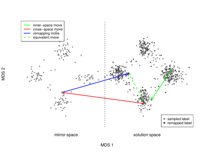
Figure 1: MDS representation of the two copies of the quotient space $\mathcal{L}/\text{\sf ord}$ using posterior samples for the political blogs example in Section 7. Arrows are described in text.

For the nuisance parameter $\pi$ we summon conjugacy to obtain

$$\pi{\,|\,}\sigma,\theta,A\sim\mbox{\sf Dir}(\alpha+\mathbf{N}(\sigma)),$$ (8)

where $\mathbf{N}(\sigma)=(N_{1},\ldots,N_{K})$ and $N_{k}$ are community sizes.

5.2 Sampling $\gamma$ and $\eta$

Sampling $\beta$ conditional on $\sigma$, $\pi$, and data $A$ is more challenging since the logistic likelihood in (2) does not specify a closed form distribution. However, if we explore a data augmentation strategy by introducing latent variables $\omega=(\omega_{ij})_{i<j:i,j\in\{1,\dots,n\}}$ from a Pólya-Gamma distribution, then the above conditional distribution of $\beta$ given $\omega$ is now available in closed form (Polson et al., 2012). More specifically, if $\omega_{ij}{\,|\,}\sigma,\beta\sim\text{\sf PG}(1,{x_{ij}(\sigma)^{\top}}\beta)$, then

$$\beta{\,|\,}\omega,\sigma,A\sim I[\gamma\leq 0]\cdot N(m,V)$$

where, with $\Omega=\text{Diag}(\omega_{ij})$ and latent weighted responses $z_{ij}=(A_{ij}-1/2)\omega_{ij}^{-1}$,

$$V=\Big{(}X^{\top}\Omega X+\frac{1}{\tau^{2}}I_{n+\binom{K}{2}}\Big{)}^{-1}\quad\text{and}\quad m=VX^{\top}\Omega z.$$ (9)

The assortativity constraint $\gamma\leq 0$ in the $\beta$ prior is clearly also present in the conditional posterior, and so we can use a simple rejection sampling step for the truncated normal: sample from unconstrained marginals $N(m,V)$ and accept only if $\gamma\leq 0$. However, since

$$\beta=\left[\begin{array}[]{c}\gamma\\ \eta\end{array}\right]\,\Bigg{|}\,\omega,\sigma,A\sim N\Bigg{(}m=\left[\begin{array}[]{c}m_{\gamma}\\ m_{\eta}\end{array}\right],V=\left[\begin{array}[]{cc}V_{\gamma}&V_{\gamma\eta}\\ V_{\eta\gamma}&V_{\eta}\end{array}\right]\Bigg{)},$$

we can adopt a more efficient way of sampling $\beta$ by first sampling $\eta$ marginally,

$$\eta{\,|\,}\omega,\sigma,A\sim N(m_{\eta},V_{\eta}),$$ (10)

and then sampling

$$\gamma{\,|\,}\eta,\omega,\sigma,A\sim I(\gamma\leq 0)\cdot N(m_{\gamma}+V_{\gamma\eta}V_{\eta}^{-1}(\eta-m_{\eta}),V_{\gamma}-V_{\gamma\eta}V_{\eta}^{-1}V_{\eta\gamma})$$ (11)

from a truncated normal. In practice, we compute the Schur complement of $V_{\eta}$, $V_{\gamma}-V_{\gamma\eta}V_{\eta}^{-1}V_{\eta\gamma}$, using the SWEEP operator (Goodnight, 1979).

5.3 Gibbs sampler

To summarize, after setting initial parameters $\sigma$, $\beta$ and $\pi$ arbitrarily, we then iterate until convergence the following Gibbs sampling steps:

1. Sample $\sigma{\,|\,}\beta,\pi,A$: for each node $i$,

   1. Sample $\sigma_{i}{\,|\,}\sigma_{[-i]},\beta,A$ from a multinomial distribution as in (7). If $N_{k}(\sigma)<2$ for some community $k$, reject and keep the previous value of $\sigma_{i}$.

   2. Remap $\sigma$ using the procedure in Section 4.

2. Sample $\pi{\,|\,}\sigma,\beta,A$ from the Dirichlet distribution in (8).

3. Sample $\beta{\,|\,}\sigma,\pi,A$:

   1. Sample $\omega{\,|\,}\sigma,\beta,\pi,A$: for each pair $i<j$, $\omega_{ij}{\,|\,}\sigma,\beta\sim\text{\sf PG}(1,x_{ij}(\sigma)^{\top}\beta)$.

   2. Sample $\beta{\,|\,}\sigma,\pi,\omega,A$: compute $m$ and $V$ as in (9), sample $\eta$ marginally as in (10), and then sample $\gamma{\,|\,}\eta$ from a truncated multivariate normal distribution as in (11).

To speed up convergence and improve precision, we set the initial $\sigma$ to be an approximate posterior mode obtained from a greedy optimization version of the above routine, similar to a gradient cyclic descent method. The main changes are:

1. In Step 1.a we take $\sigma_{i}$ to be the mode of $\sigma_{i}{\,|\,}\sigma_{[-i]},\beta,A$ (but we might still reject $\sigma_{i}$ if $N_{k}(\sigma)<2$ for some $k$ and remap $\sigma$ in Step 1.b.)

2. In Step 2, we take $\pi$ to be the mode of the Dirichlet distribution in (8).

3. Step 3 is substituted by a regularized iterative reweighted least-squares (IRLS) step. IRLS is usual when fitting logistic regression models (McCullagh and Nelder, 1989). At the $t$-th iteration we define $\mu_{ij}=\text{logit}^{-1}(x_{ij}(\sigma)^{\top}\beta^{(t)})$ and $W=\text{Diag}(\mu_{ij}(1-\mu_{ij}))$ to obtain the update

   $$V=\Big{(}X^{\top}WX+\frac{1}{\tau^{2}}I_{n+\binom{K}{2}}\Big{)}^{-1}\quad\text{and}\quad\beta^{(t+1)}=VX^{\top}Wz^{(t)}$$

   where $z^{(t)}=X\beta^{(t)}+W^{-1}(y-\mu)$ is now the “working response”. To guarantee that the community constraints $\gamma\leq 0$ are met, we use an active-set method (Nocedal and Wright, 2006, Chapter 16).

Since we expect the posterior space to be multimodal, we adopt a strategy similar to Karrer and Newman (2011) and sample multiple starting points for $\sigma$ according to its prior distribution and then obtain approximate posterior modes for each simulation. We elect the best approximate mode over all simulations as the starting point for the Gibbs sampler, which is then run until convergence to more thoroughly explore the posterior space. For convenience, the Gibbs sampler and its optimization version are implemented in the R package sbmlogit, available as supplementary material.

6 Posterior Inference

The usual estimator for label assignment is the maximum a posteriori (MAP) estimator,

$$\widehat{\sigma}_{M}=\mathop{\rm arg\,min}\limits_{\widetilde{\sigma}\in\{1,\ldots,K\}^{n}}{\mathbb{E}}_{\sigma{\,|\,}A}\big{[}I(\widetilde{\sigma}\neq\sigma)\big{]}=\mathop{\rm arg\,max}\limits_{\widetilde{\sigma}\in\{1,\ldots,K\}^{n}}{\mathbb{P}}(\sigma=\widetilde{\sigma}{\,|\,}A),$$

which, albeit based on a zero-one loss function (Besag, 1986), has the advantage of being invariant to label permutations. However, given the flexibility in our model due to the hierarchical levels, the posterior space is often complex and so the MAP might fail to capture the variability and might focus on sharp peaks that gather a small amount of posterior mass around them.

Another estimator for label assignment arises from minimizing Binder’s loss $B$ (Binder, 1978, 1981),

$$\widehat{\sigma}_{B}=\mathop{\rm arg\,min}\limits_{\widetilde{\sigma}\in\{1,\ldots,K\}^{n}}{\mathbb{E}}_{\sigma{\,|\,}A}\big{[}B(\widetilde{\sigma},{\sigma})\big{]},$$ (12)

where

$$B(\widetilde{\sigma},{\sigma})=\sum_{i<j}I(\widetilde{\sigma}_{i}\neq\widetilde{\sigma_{j}})I(\sigma_{i}=\sigma_{j})+I(\widetilde{\sigma}_{i}=\widetilde{\sigma_{j}})I(\sigma_{i}\neq\sigma_{j}).$$

The advantage of Binder’s loss is that since it penalizes pairs of nodes it is invariant to label permutations—that is, $B(\widetilde{\sigma},\sigma)=B(\widetilde{\sigma},\phi(\sigma))=B(\phi(\widetilde{\sigma}),\sigma)$ for any permutation $\phi$. However, Lau and Green (2007) have shown that minimizing Binder’s loss is equivalent to binary integer programming, which is an NP-hard problem. Moreover, as Fritsch and Ickstadt (2009) point out, even the approximated solution given by Lau and Green (2007) is only feasible when the dataset is of moderate size.

In contrast, when compared to MAP inference, centroid estimation (Carvalho and Lawrence, 2008) offers a better representative of the space since it arises from a loss function that is more refined:

$$\widehat{\sigma}_{H}=\mathop{\rm arg\,min}\limits_{\widetilde{\sigma}\in\{1,\ldots,K\}^{n}}{\mathbb{E}}_{\sigma{\,|\,}A}\big{[}H(\widetilde{\sigma},\sigma)\big{]},$$

where $H$ is Hamming distance, $H(\widetilde{\sigma},\sigma)=\sum_{i=1}^{n}I(\widetilde{\sigma}_{i}\neq\sigma_{i})$. The centroid estimator also identifies the median probability model, and thus is known to offer better predictive resolution that the MAP estimator (Barbieri and Berger, 2004). However, Hamming loss is only invariant to double label permutations but not to single label permutations, i.e., $H(\widetilde{\sigma},\sigma)=H(\phi(\widetilde{\sigma}),\phi(\sigma))$ but it is not necessarily true that $H(\widetilde{\sigma},\sigma)=H(\phi(\widetilde{\sigma}),\sigma)$ or $H(\widetilde{\sigma},\sigma)=H(\widetilde{\sigma},\phi(\sigma))$, and thus, in order for Hamming loss to be meaningful for estimation when the labels are non-identifiable we need to account for label aliasing. We then redefine the centroid estimator to depend on a specific permutation, for instance the canonical permutation $\rho$ in (6),

$$\widehat{\sigma}_{C}=\rho\Bigg{(}\mathop{\rm arg\,min}\limits_{\widetilde{\sigma}\in\{1,\ldots,K\}^{n}}{\mathbb{E}}_{\sigma{\,|\,}A}\big{[}H(\widetilde{\sigma},\rho(\sigma))\big{]}\Bigg{)}.$$

This remapped centroid estimator considers only one version of the posterior space, namely the reference quotient space $\mathcal{L}/\text{\sf ord}$ with ord in (5). The main advantage of this new estimator is to allow the following characterization (see Appendix 9.3 for the proof):

Theorem 2.

The centroid estimator $\widehat{\sigma}_{C}$ is a mapped consensus estimator: if ${\mathbb{P}}^{*}(\sigma{\,|\,}A)$ is the induced posterior probability of $\sigma\in\mathcal{L}\,/\,\mbox{\sf ord}$ and

$$(\widehat{\sigma}^{*})_{i}=\mathop{\rm arg\,max}\limits_{k\in\{1,\ldots,K\}}{\mathbb{P}}^{*}(\sigma_{i}=k{\,|\,}A)$$

then $\widehat{\sigma}_{C}=\rho(\widehat{\sigma}^{*})$.

In practice, we estimate

$$\widehat{{\mathbb{P}}}^{*}(\sigma_{i}=k{\,|\,}A)\approx\frac{1}{N}\sum_{t=1}^{N}I(\sigma^{(t)}_{i}=k)$$

using the realizations from the Gibbs sampler presented in Section 5 to define $\widehat{\sigma}_{C}$. Since we only need to elect, for each actor, the most likely label, obtaining the centroid estimator is much simpler computationally than MAP and Binder estimation. Note that due to the remap step when sampling $\sigma{\,|\,}\theta,A$, we are always constrained to the quotient space $\mathcal{L}/\mbox{\sf ord}$ and identifying label realizations under $\rho$, and thus really approximating ${\mathbb{P}}^{*}(\sigma{\,|\,}A)$.

6.1 Relating Binder and Centroid Estimators

We start by noting that if we define an extended matched map $M(\sigma)=\{I(\sigma_{i}=\sigma_{j})\}_{1\leq i<j\leq n}$ that makes pairwise comparisons among labels in $\sigma$, then Binder and Hamming losses are related through $B(\widetilde{\sigma},\sigma)=H(M(\widetilde{\sigma}),M(\sigma))$ and so Binder’s estimator in (12) is also a centroid estimator in the extended matched space $M(\mathcal{L})$.

Back to the original space $\mathcal{L}$ of labels, we observe that, in practice, the Binder and centroid estimators are often close (in either loss.) To explain these observations, we need the next result relating Binder and Hamming losses (the proof can be found in Appendix 9.4):

Theorem 3.

For any pair of label assignments $\widetilde{\sigma}$ and ${\sigma}$, Binder loss is bounded by Hamming loss through

$$B(\widetilde{\sigma},{\sigma})\leq H(\widetilde{\sigma},{\sigma})\Big{(}n-\frac{1}{2}H(\widetilde{\sigma},{\sigma})\Big{)}.$$ (13)

Moreover, if $K=2$ then $B(\widetilde{\sigma},\sigma)=H(\widetilde{\sigma},\sigma)(n-H(\widetilde{\sigma},\sigma))$.

From (13) we see that Binder’s loss can be approximately linearly bounded by Hamming loss when the Hamming distance between $\widetilde{\sigma}$ and ${\sigma}$ is small. Thus, when the marginal posterior distribution on $\sigma$ has a compact cluster of label configurations with high posterior mass we expect this cluster to contain the centroid estimator and also, according to (13), the Binder estimator since minimizing the posterior expected Hamming loss is approximately equivalent to minimizing the posterior expected Binder loss in this case. In the next section we run experiments on simulated datasets and observe that the two estimators are often close and show similar performance for simple networks (check, for instance, Figure 5.)

7 Experimental Results

In this section, we demonstrate the performance of the centroid estimator and compare it to Binder estimator under our model and to KN estimator (Karrer and Newman, 2011), Fast-Greedy (FG) estimator (Clauset et al., 2004), Multi-Level (ML) estimator (Blondel et al., 2008), Walktrap (WT) estimator (Pons and Latapy, 2004) and Label Propagation (LP) estimator (Raghavan et al., 2007) through an empirical study and two case studies. In the case studies we run repeated experiments on the same dataset and obtain the error rates of the estimators mentioned above when compared to known or bona fide ground truth references. To compare those estimators, we define a $q$-error interval as the interval with endpoints being the $q/2$ and $1-q/2$ quantiles of the error rates.

Before discussing the experimental results, we present two illustrative examples next.

7.1 Illustrative Examples

Even though the models reviewed above are flexible enough to identify social block structure, they might fail to actually recognize communities. We now show two simple examples to demonstrate how this happens, and compare our proposed solution to the results from applying Karrer and Newman’s (KN) popular degree-corrected SBM (Karrer and Newman, 2011).

The first dataset is a synthetic network, denoted as the “spike” dataset, which we intentionally designed to show that degree correction is not sufficient to elicit communities. The network considered is split into $K=2$ communities. The first community contains $2n_{1}$ nodes with $n_{1}$ of them being strongly connected as a complete graph $K_{n_{1}}$ (a “kernel”) and having a one-to-one connection with the remaining $n_{1}$ nodes (a “crown”). The other community is formed in a similar way, but with a complete $K_{rn_{1}}$ kernel connected to a $rn_{1}$ crown, totalling $2rn_{1}$ nodes (see Figure 2). We add some between-community edges in such a way that each node from the complete graph $K_{n_{1}}$ in the first community is connected to $r$ nodes from the complete graph $K_{rn_{1}}$ in the second community.

We note that this network can still be characterized as having a community behavior since the edge density between communities is smaller than the density within communities. Moreover, due to the crowns, we also need to account for degree heterogeneity in each community. Let us then consider the case when $n_{1}=10$ and $r=5$. Figure 2 compares the KN estimator and our estimator. The kernel-crown structure of both communities is not reflected in KN estimator; moreover, there are more edges between groups than within groups, which is not prescribed by community behavior.

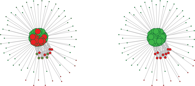
Figure 2: Spike network, $n_{1}=10$, $r=5$. Node sizes are proportional to degree; node colors (red/green) represent groups in KN estimator (left) and our estimator (right.) Node borders mark the reference.

We observe that degree correction is not enough to correctly capture the community structure in the synthetic network that we designed. However, similar results are also observed in some real-world datasets. Consider, for example, the “sampson” network reported by Sampson (1968) at time point $T_{4}$ among a group of $18$ trainee monks at a New England monastery. Four types of relations—affection, esteem, influence, and sanctioning—between the monks are collected. In this network, each node represents a monk in the monastery, and two nodes are considered to be connected if they considered each other as being in at least one of the four relations when asked by Sampson. Sampson reported a partition of trainee monks into three communities ($K=3$): Young Turks, Loyal Opposition and Outcasts. Figure 3 compares KN estimator to our estimator and shows a similar pattern where within group connections are sparser than between group connections according to the KN estimate; in particular, there are more edges between the red and green communities than within the green community. In fact, the KN partition does not agree with any well-accepted reference.

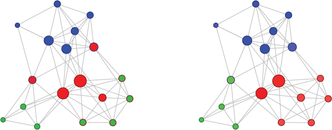
Figure 3: Sampson network at $T_{4}$, $n=18$. Node sizes are proportional to degree; node colors mark KN estimator (left) and our estimator (right). Node borders mark the reference.

7.2 Empirical Study

First, we evaluate our estimator on simulated datasets with known references. The networks are generated from a class of benchmark graphs that account for heterogeneities in node degree distributions and community sizes Lancichinetti et al. (2008). The model used in the simulation considers the following parameters: both degree distribution and the community sizes are assumed to follow power law distributions with exponents $a$ and $b$, respectively; each network consists of $n$ nodes and has average degree $\langle k\rangle$; and mixing parameter $\mu$ represents the proportion of the between-community edges.

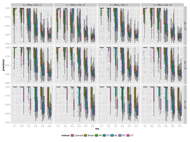
Figure 8: Benchmark networks of $n=100$ nodes, with different combinations of the exponents $a\in\{2,3\}$, $b\in\{1,2\}$ and the average degree $\langle k\rangle\in\{10,15,25\}$ are used. Each boxplot corresponds to the precision of the estimator over 100 graph realizations.

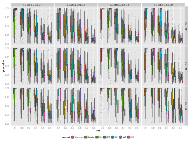
Figure 9: Benchmark networks of $n=500$ nodes, with different combinations of the exponents $a\in\{2,3\}$, $b\in\{1,2\}$ and the average degree $\langle k\rangle\in\{10,15,25\}$ are used. Each boxplot corresponds to the precision of the estimator over 100 graph realizations.

We simulate $100$ networks for each combination of $n=(100,500)$, $a=(2,3)$, $b=(1,2)$, and $\mu=(0.1,0.2,0.3,0.4,0.5,0.6)$. Figure 4 shows one realization of the benchmark networks as an example. The precision of the centroid, Binder, KN, FG, ML, WT and LP estimators are summarized in Figure 5. We observe from the figure that the centroid estimator yields smaller error rates than the KN estimator while performing slightly better than Binder estimator in terms of mean error rate. Besides, the centroid estimator performs comparably to FG, ML, WT and LP estimators when the mixing parameter $\mu$ is small but outperforms these four estimators to a large extent when the mixing parameter or the average degree is relatively large. Not surprisingly, all estimators perform worse as the mixing parameter $\mu$ increases (so that the communities are defined in a weaker sense) or the average degree $\langle k\rangle$ decreases. Similar results are found under other different combinations of $(a,b,\langle k\rangle)$, as shown in Figure 8 and Figure 9 in the Appendix.

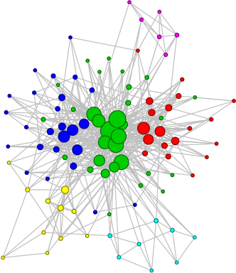
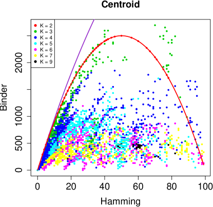
Figure 4: Left: one realization of the benchmark networks with $n=100$ nodes, $a=2$, $b=1$, $\mu=0.4$, and $\langle k\rangle=10$. Right: Binder loss against Hamming loss tested on 50 graph realizations of such benchmark networks. Colors mark different values of $K$. Lines correspond to the upper bound in (13) for $K>2$ and $K=2$.

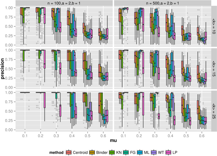
Figure 5: Benchmark networks of $n=100$ and $500$ nodes, with different combinations of the exponents $a$, $b$ and the average degree $\langle k\rangle$ are used. Each boxplot corresponds to the precision of the estimator over 100 and 50 graph realizations for $n=100$ and $n=500$, respectively.

7.3 Case Study

Next, we evaluate our estimator for community detection on two real-world network datasets.

7.3.1 Political blogs

The first case study is the political blogs network (Adamic and Glance, 2005), which is a medium real-world network containing over one thousand nodes. In this network, each node is a blog over the period of two months preceding the U.S. Presidential Election of 2004, and two nodes are considered to be connected if they referred to one another and there was overlap in the topics they discussed. The network is known to be split into two communities ($K=2$), liberals and conservatives, and has $n=1,\!222$ nodes after isolated nodes are removed. It is expected that blogs in favor of the same party are more likely to be linked and discussing the same topics than those in favor of different parties, which corroborates a community behavior.

The centroid estimator, depicted in the leftmost panel in Figure 6, agrees well with the reference of this network. We estimate each $\eta_{i}$ for node $i$ by its estimated posterior mean using the converged samples and plot the estimated $\eta_{i}$ against the logit normalized degree of node $i$ in the middle panel of Figure 6. There is a positive linear relationship between $\eta_{i}$ and the logit of the normalized degrees, indicating that the expected degree, thus the probability of having an edge, is positively related to the observed degree of the node. If there is a community effect, that is, if the network can be better explained by partitioning nodes into two different communities, then $\gamma_{12}$ is expected to be significantly negative. The rightmost panel in Figure 6 shows the estimated posterior distribution of $\gamma_{12}$. An estimated 95% credible interval for $\gamma$ is $[-3.16,-2.99]$, which shows a clear deviation from $0$ and thus indicates a strong community effect in the network.

We further compare the centroid estimator with two other estimators, Binder and KN, as in the previous section. The estimated $90\%$ error intervals for the centroid, Binder, and KN estimators are $[0.053,0.054]$, $[0.053,0.054]$, and $[0.045,0.051]$, respectively. In general, the three estimators perform equally well while the KN estimator yields a slightly smaller error rate on average.

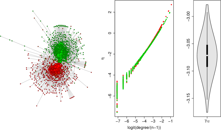
Figure 6: Political blogs network. Left: Node sizes are proportional to degree; node colors signal the centroid estimators (red/green). Node color intensities are proportional to $\widehat{{\mathbb{P}}}^{*}(\sigma_{i}{\,|\,}A)$ and node borders mark the reference. Middle: $\eta_{i}$ on logit$(\mbox{degree}_{i}/(n-1))$ for each node $i$; color for each node $i$ represents ${(\widehat{\sigma}_{C})}_{i}$. Right: estimated posterior distribution for $\gamma_{12}$.

7.3.2 Political books

Finally, we pick the political books dataset compiled by Valdis Krebs (unpublished). This is a network of political books sold by the on-line bookseller Amazon around the time of the US presidential election in 2004. The network is split into three communities: liberal, neutral, or conservative. An edge between two books represents frequent co-purchasing by the same buyers. We also use weakly-informative priors and run multiple chains. The estimated $90\%$ error intervals for the centroid, Binder, and KN estimators are $[0.167,0.175]$, $[0.167,0.175]$, and $[0.171,0.171]$, respectively. The reason why we observe large error rates under all estimation procedure analyzed here might be that the reference provided by Valdis Krebs is not that reliable, or that misclassified books appeal to buyers who purchase books from all three political opinions. Most of the misclassified nodes are in the neutral (red) community.

Figure 7 shows the centroid estimator of the political books network in the right panel. The communities corresponding to liberal (blue) and conservative (green) are clearly separated by the neutral (red) community and agree with the reference well. The middle panel plots estimated $\eta_{i}$ against normalized degrees in logit scale; it is evident that the in-between red community has a different intercept for $\eta$, indicating that it is less connected. The right panel shows estimated marginal posterior distributions for $\gamma$. Not surprisingly, $\gamma_{23}<\gamma_{12}$ and $\gamma_{23}<\gamma_{13}$ with high posterior probability since communities $2$ (green) and $3$ (blue) are separated by community $1$ (red) and so do not share many edges.

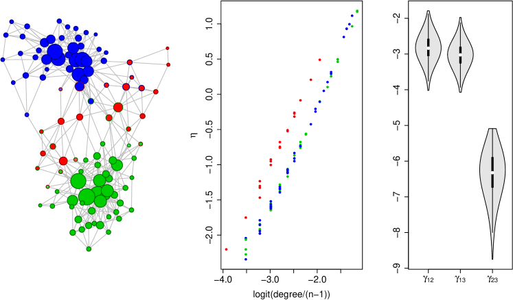
Figure 7: Political books network. Left: node sizes are proportional to degree; node colors signal the centroid estimators. Node color intensities are proportional to $\widehat{{\mathbb{P}}}^{*}(\sigma_{i}{\,|\,}A)$ and node borders mark the reference. Middle: $\eta_{i}$ on logit$(\mbox{degree}_{i}/(n-1))$ for each node $i$; color for each node $i$ represents ${(\widehat{\sigma}_{C})}_{i}$. Right: estimated posterior distribution for $\gamma$.

8 Discussion

In this paper we have proposed a Bayesian model based on degree-corrected stochastic blockmodels that is tailored for community detection. More specifically, our model is flexible due to its hierarchical structure and aims to capture the gregarious community behavior by requiring, through prior specification, that the probability of within-community associations to be no smaller than the probability of between-community associations. Moreover, we argue that the model is a better representative of assortatively mixing networks with binary data coding the associations instead of frequency counts, since we model binary observations using a suitable logistic regression with parameters for within and between-community probabilities of association. We devise a Gibbs sampler to obtain posterior samples and exploit a latent variable formulation to yield closed-form conditionals.

We formally address label identifiability by restricting label configurations to a canonical reference subspace, and propose a remap procedure to implement this constraint in practice. As a consequence, labels are interpretable and we are able to estimate any function of the labels as opposed to previous approaches that were restricted to permutation-invariant functions. In particular, we propose a novel remapped centroid estimator to infer community assignments. We contend that while the model can arguably represent the data well, the posterior space can be complex and a bad estimator can spoil the analysis; it is then imperative to adopt an estimator that arises from a principled and refined loss function and thus better summarizes the posterior space. Our proposed remapped centroid estimator is more similar to a posterior mean, and thus, while considering the whole posterior distribution in the space of remapped label assignments, tends to situate itself in regions of high concentration of posterior mass. From a practical point of view, we show that the proposed estimator performs better than MAP and Binder estimators and achieves lower misclassification rates.

If the posterior space is multimodal then a single point estimator has difficulty in representing the space, and the centroid estimator is not immune to this problem. We intend to further extend the proposed estimation procedure to account for multiple modes by exploring conditional estimators on partitions of the space. While this can be done empirically by clustering posterior samples, we will pursue a more principled way of identifying partitions. As simple extensions to the proposed model, we also intend to incorporate parameters for node attributes and to generalize the formulation to account for count, categorical, and ordinal data. Other directions for future work, albeit not related to community detection, include extending the remap procedure to other settings such as clustering and mixture model inference.

9 Appendix

9.1 Proof of Theorem 1

For the proof we first note that we can split each row $x_{ij}$ in the design matrix of (2) according to $\gamma$ and $\eta$ entries, $x_{ij}\doteq[b_{ij}\quad c_{ij}]$, where

$$b_{ij,kl}=I[\min(\sigma_{i},\sigma_{j})=k,\max(\sigma_{i},\sigma_{j})=l], \qquad k,l=1,\ldots,K,k\leq l,$$ (14)

$$c_{ij,v}=I(i=v)+I(j=v), \qquad v=1,\ldots,n,$$

that is, $b_{ij}$ identifies the pair of communities at the endpoints of $(i,j)$ for $\gamma$ and $c_{ij}$ marks each node-correction from $\eta$.

Proof of (a).

Let us pick an arbitrary community $k$ and a pair $(i,j)$. There are then three ways to classify $(i.j)$: (i) it is either outside of community $k$; (ii) one of its endpoints is in community $k$; or (iii) it is inside community $k$. If we now define $d_{ij,k}=\sum_{v:\sigma_{v}=k}c_{ij,v}$ then $(i,j)$ is classified exactly according to $d_{ij,k}$: $d_{ij,k}=0,1,$ or $2$ if $(i,j)$ is in cases (i), (ii), or (iii), respectively. Thus, it follows that

$$2b_{ij,kk}+\sum_{l\neq k}b_{ij,kl}=\sum_{v:\sigma_{v}=k}c_{ij,v},$$

for each $k=1,\ldots,K$, and so $X$ has $K$ constraints in its columns. ∎

Proof of (b).

Note that $X$ is full column-ranked if and only if $X^{\top}X$ is invertible, so we just need to show that $X^{\top}X$ is invertible if $N_{k}\geq 2$ for $k=1,\dots,K$. Let $B=[b_{ij,12},\dots,b_{ij,K-1K}]_{i<j}$ and $C=[c_{ij,1},\dots,c_{ij,n}]_{i<j}$. Then $X=[B,C]$ and

$$X^{\top}X=\left[\begin{array}[]{cc}B^{\top}B&B^{\top}C\\ C^{\top}B&C^{\top}C\end{array}\right].$$

Thus, $X^{\top}X$ is invertible if and only if both $B^{\top}B$ and the Schur complement of $C^{\top}C$, $\Delta\doteq C^{\top}[I-B(B^{\top}B)^{-1}B^{\top}]C$ are invertible. First,

$$B^{\top}B=\text{Diag}\Bigg{(}\sum_{i<j}I[{\sigma_{i}=k,\sigma_{j}=l}\text{ or }{\sigma_{i}=l,\sigma_{j}=k}]\Bigg{)}=\text{Diag}(N_{k}N_{l}),$$

and so, for this diagonal matrix to be invertible we need $N_{k}\neq 0$ for $k=1,\dots,K$.

As for the Schur complement $\Delta$, we have that

$$\Delta_{ii}=n-1-\sum_{k\neq i}\frac{\sum_{l\neq i}I[\sigma_{i}\neq\sigma_{k}=\sigma_{l}]}{N_{\sigma_{i}}N_{\sigma_{k}}},$$

and, for $i<j$,

$$\Delta_{ij}=1-\sum_{k\neq i}\frac{\sum_{l\neq j}I[\sigma_{i}=\sigma_{j}\neq\sigma_{k}=\sigma_{l}\text{ or }\sigma_{i}=\sigma_{l}\neq\sigma_{k}=\sigma_{j}]}{N_{\sigma_{i}}N_{\sigma_{k}}}.$$

But if $\sigma_{i}\neq\sigma_{j}$,

$$\Delta_{ij}=1-\sum_{k\neq i}\frac{\sum_{l\neq j}I[\sigma_{i}=\sigma_{l}\neq\sigma_{k}=\sigma_{j}]}{N_{\sigma_{i}}N_{\sigma_{k}}}=0,$$

and otherwise, if $\sigma_{i}=\sigma_{j}$,

$$\Delta_{ij}=1-\sum_{k\neq i}\frac{\sum_{l\neq i}I[\sigma_{i}\neq\sigma_{k}=\sigma_{l}]}{N_{\sigma_{i}}N_{\sigma_{k}}},$$ (15)

and so $\Delta_{ii}-\Delta_{ij}=n-2$. Thus, after some row and column operations, $\Delta$ can be written as a block diagonal matrix where each block of size $N_{k}$ has the form:

$$\left[\begin{array}[]{cccc}p&q&\dots&q\\ q&p&\dots&q\\ \vdots&&\ddots&\vdots\\ q&q&\dots&p\end{array}\right]$$

with $q=\Delta_{ij}$ in (15) and $p=n-2+q$. The determinant of the block diagonal matrix is nonzero if and only if $n\neq 2$ and $N_{k}\neq 1$. Moreover, the determinant of $X^{\top}X$ is the same as that of the block diagonal matrix since one can be obtained from the other through row and column operations. Thus, the conditions $N_{k}\neq 0$ from $B^{\top}B$ and now $N_{k}\neq 1$ can be summarized into $N_{k}\geq 2$. ∎

9.2 Remap Algorithm

Algorithm 1 lists a routine that finds the canonical map $\rho$ based on the canonical order in $\sigma$ as in Equation (6) and remaps $\sigma$ in-place.

Algorithm 1 Remapping labels in $\sigma$ to $\rho(\sigma)$.

  assigned $\leftarrow\{\}$

  $\rho\leftarrow\{\}$

  $n\leftarrow 0$ {number of different labels in $\sigma$}

  for $i=1,\ldots,|\sigma|$ do {obtain $\rho\doteq$ ord$(\sigma)^{-1}$}

     if not assigned$(\sigma(i))$ then {first appearance?}

        assigned$(\sigma(i))\leftarrow$ true {mark $\sigma(i)$}

        $n\leftarrow n+1$

        $\rho(\sigma(i))\leftarrow n$

     end if

  end for

  for $i=1,\ldots,|\sigma|$ do {remap $\sigma$}

     $\sigma(i)\leftarrow\rho(\sigma(i))$

  end for

  return $\sigma$

9.3 Proof of Theorem 2

It is sufficient to find the pre-map estimator

$$\widehat{\sigma}^{*}\doteq\mathop{\rm arg\,min}\limits_{\widetilde{\sigma}\in\{1,\ldots,K\}^{n}}{\mathbb{E}}_{\sigma{\,|\,}A}\big{[}H(\widetilde{\sigma},\rho(\sigma))\big{]}$$

since, by definition, $\widehat{\sigma}_{C}=\rho(\widehat{\sigma}^{*})$.

Denoting $\Sigma=\{1,\ldots,K\}^{n}$ and $\Sigma^{*}=\Sigma\,/\,\mbox{\sf ord}$, we have that

$$\begin{split}{\mathbb{E}}_{\sigma{\,|\,}A}\big{[}H(\widetilde{\sigma},\rho(\sigma))\big{]}&=\sum_{\sigma\in\Sigma}H(\widetilde{\sigma},\rho(\sigma)){\mathbb{P}}(\sigma{\,|\,}A)\\ &=\sum_{\sigma\in\Sigma^{*}}\sum_{\sigma^{*}:\rho(\sigma^{*})=\sigma}H(\widetilde{\sigma},\sigma){\mathbb{P}}(\sigma^{*}{\,|\,}A).\\ \end{split}$$

Since ${\mathbb{P}}(\sigma^{*}{\,|\,}A)={\mathbb{P}}(\sigma{\,|\,}A)$ follows from the lack of identifiability we further obtain

$${\mathbb{E}}_{\sigma{\,|\,}A}\big{[}H(\widetilde{\sigma},\rho(\sigma))\big{]}=\sum_{\sigma\in\Sigma^{*}}n(\sigma)H(\widetilde{\sigma},\sigma){\mathbb{P}}(\sigma{\,|\,}A),$$

where $n(\sigma)=|\{\sigma^{*}:\rho(\sigma^{*})=\sigma\}|=K!/(K-k(\sigma))!$ is the number of assignments that are identified to $\sigma$ through ord, and $k(\sigma)$ is the number of different labels in $\sigma$. We can then define ${\mathbb{P}}^{*}(\sigma{\,|\,}A)\doteq n(\sigma){\mathbb{P}}(\sigma{\,|\,}A)$ as the induced measure in the quotient space $\Sigma^{*}$ to thus have

$${\mathbb{E}}_{\sigma{\,|\,}A}\big{[}H(\widetilde{\sigma},\rho(\sigma))\big{]}=\sum_{\sigma\in\Sigma^{*}}H(\widetilde{\sigma},\sigma){\mathbb{P}}^{*}(\sigma{\,|\,}A)=\sum_{\sigma\in\Sigma^{*}}\sum_{i=1}^{n}I(\widetilde{\sigma}_{i}\neq\sigma_{i}){\mathbb{P}}^{*}(\sigma{\,|\,}A)\\ =n-\sum_{i=1}^{n}\sum_{\sigma\in\Sigma^{*}}I(\widetilde{\sigma}_{i}=\sigma_{i}){\mathbb{P}}^{*}(\sigma{\,|\,}A)=n-\sum_{i=1}^{n}{\mathbb{P}}^{*}(\sigma_{i}=\widetilde{\sigma}_{i}{\,|\,}A).$$

But then

$$\mathop{\rm arg\,min}\limits_{\widetilde{\sigma}\in\{1,\ldots,K\}^{n}}{\mathbb{E}}_{\sigma{\,|\,}A}\big{[}H(\widetilde{\sigma},\rho(\sigma))\big{]}=\mathop{\rm arg\,max}\limits_{\widetilde{\sigma}\in\{1,\ldots,K\}^{n}}\sum_{i=1}^{n}{\mathbb{P}}^{*}(\sigma_{i}=\widetilde{\sigma}_{i}{\,|\,}A)$$

and so

$$(\widehat{\sigma}^{*})_{i}=\mathop{\rm arg\,max}\limits_{k\in\{1,\ldots,K\}}{\mathbb{P}}^{*}(\sigma_{i}=k{\,|\,}A),$$

that is, $\widehat{\sigma}^{*}$ is a consensus estimator, as desired.

9.4 Proof of Theorem 3

To compare $\widetilde{\sigma}$ and $\sigma$ let us define $n_{ij}\doteq\sum_{k,l}I(\sigma_{k}=i,\widetilde{\sigma}_{l}=j)$, the number of nodes that belong to community $i$ in $\sigma$ and to community $j$ in $\widetilde{\sigma}$. Then, $B(\widetilde{\sigma},\sigma)=\sum_{i}\sum_{j<k}(n_{ij}n_{ik}+n_{ji}n_{ki})$, $H(\widetilde{\sigma},\sigma)=\sum_{i\neq j}n_{ij}$, and $n=\sum_{i,j}n_{ij}$.

For instance, if $K=2$ then $H(\widetilde{\sigma},{\sigma})=n_{12}+n_{21}$ and

$$\begin{split}B(\widetilde{\sigma},{\sigma})&=(n_{11}n_{12}+n_{21}n_{22})+(n_{11}n_{21}+n_{12}n_{22})\\ &=(n_{12}+n_{21})(n_{11}+n_{22})\\ &=H(\widetilde{\sigma},{\sigma})\big{(}n-H(\widetilde{\sigma},{\sigma})\big{)}.\end{split}$$

More generally, for $K>2$, we have:

$$\begin{split}nH(\widetilde{\sigma},{\sigma})&=\sum_{i\neq j}n_{ij}\sum_{i,j}n_{ij}=\sum_{i\neq j}n_{ij}\Bigg{(}\sum_{i\neq j}n_{ij}+\sum_{i}n_{ii}\Bigg{)}\\ &=\sum_{i\neq j}n_{ij}\sum_{i\neq j}n_{ij}+\sum_{i\neq j}n_{ij}\sum_{i}n_{ii}\\ &=\underbrace{\sum_{i\neq j}n_{ij}^{2}}_{A}+\underbrace{\sum_{\begin{subarray}{c}i\neq j,k\neq l\\ k\neq i,j\neq l\end{subarray}}n_{ij}n_{kl}}_{B}+2\underbrace{\sum_{\begin{subarray}{c}i\neq j,i\neq k\\ j<k\end{subarray}}(n_{ij}n_{ik}+n_{ji}n_{ki})}_{C}\\ &\qquad+\underbrace{\sum_{\begin{subarray}{c}i\neq j,i\neq k\\ j\neq k\end{subarray}}n_{ii}n_{jk}}_{D}+\underbrace{\sum_{i\neq j}(n_{ii}n_{ij}+n_{ii}n_{ji})}_{E}.\end{split}$$

Thus, $B(\widetilde{\sigma},\sigma)=C+E$ and, in particular,

$$\begin{split}H^{2}(\widetilde{\sigma},{\sigma})&=\Big{(}\sum_{i\neq j}n_{ij}\Big{)}\Big{(}\sum_{i\neq j}n_{ij}\Big{)}\\ &=\sum_{i\neq j}n_{ij}^{2}+\sum_{\begin{subarray}{c}i\neq j,k\neq l\\ k\neq i,j\neq l\end{subarray}}n_{ij}n_{kl}+2\sum_{\begin{subarray}{c}i\neq j,i\neq k\\ j<k\end{subarray}}(n_{ij}n_{ik}+n_{ji}n_{ki})\\ &=A+B+2C.\end{split}$$

The bound $B(\widetilde{\sigma},\sigma)\leq H(\widetilde{\sigma},\sigma)(n-H(\widetilde{\sigma},{\sigma})/2)$ then follows from

$$nH(\widetilde{\sigma},{\sigma})-B(\widetilde{\sigma},{\sigma})-\frac{1}{2}H^{2}(\widetilde{\sigma},{\sigma})=\frac{1}{2}A+\frac{1}{2}B+D\geq 0$$

since $A,B$ and $D$ are all non-negative.

References

- Adamic and Glance (2005) Adamic, L. and N. Glance (2005). The political blogosphere and the 2004 US election: Divided they blog. In Proceedings of the 3rd International Workshop on Link Discovery, pp. 36–43.
- Airoldi et al. (2008) Airoldi, E. M., D. M. Blei, S. E. Fienberg, and E. P. Xing (2008). Mixed membership stochastic blockmodels. The Journal of Machine Learning Research 9, 1981–2014.
- Albert and Barabási (2002) Albert, R. and A.-L. Barabási (2002, Jan). Statistical mechanics of complex networks. Rev. Mod. Phys. 74, 47–97.
- Anderson et al. (1992) Anderson, C., S. Wasserman, and K. Faust (1992). Building stochastic blockmodels. Social Networks 14(1), 137–161.
- Barbieri and Berger (2004) Barbieri, M. and J. Berger (2004). Optimal predictive model selection. The Annals of Statistics 32(3), 870–897.
- Barnes (1982) Barnes, E. (1982). An algorithm for partitioning the nodes of a graph. SIAM Journal on Algebraic Discrete Methods 3(4), 541–550.
- Besag (1986) Besag, J. (1986). On the statistical analysis of dirty pictures. Journal of the Royal Statistical Society. Series B (Methodological) 48(3), 259–302.
- Bickel and Chen (2009) Bickel, P. and A. Chen (2009). A nonparametric view of network models and Newman–Girvan and other modularities. Proceedings of the National Academy of Sciences 106(50), 21068–21073.
- Bickel et al. (2013) Bickel, P., D. Choi, X. Chang, and H. Zhang (2013, 08). Asymptotic normality of maximum likelihood and its variational approximation for stochastic blockmodels. The Annals of Statistics 41(4), 1922–1943.
- Binder (1978) Binder, D. A. (1978). Bayesian cluster analysis. Biometrika 65(1), 31–38.
- Binder (1981) Binder, D. A. (1981). Approximations to bayesian clustering rules. Biometrika 68(1), 275–285.
- Blondel et al. (2008) Blondel, V. D., J.-L. Guillaume, R. Lambiotte, and E. Lefebvre (2008). Fast unfolding of communities in large networks. Journal of Statistical Mechanics: Theory and Experiment 2008(10), P10008.
- Brandes et al. (2007) Brandes, U., D. Delling, M. Gaertler, R. Görke, M. Hoefer, Z. Nikoloski, and D. Wagner (2007). On finding graph clusterings with maximum modularity. In Graph-Theoretic Concepts in Computer Science, pp. 121–132. Springer.
- Carvalho and Lawrence (2008) Carvalho, L. and C. Lawrence (2008). Centroid estimation in discrete high-dimensional spaces with applications in biology. Proceedings of the National Academy of Sciences 105(9), 3209–3214.
- Celisse et al. (2012) Celisse, A., J.-J. Daudin, and L. Pierre (2012). Consistency of maximum-likelihood and variational estimators in the stochastic block model. Electronic Journal of Statistics 6, 1847–1899.
- Choi et al. (2012) Choi, D. S., P. J. Wolfe, and E. M. Airoldi (2012). Stochastic blockmodels with a growing number of classes. Biometrika.
- Clauset et al. (2004) Clauset, A., M. E. J. Newman, and C. Moore (2004, August). Finding community structure in very large networks. Physical Review E 70(6), 066111+.
- Daudin et al. (2008) Daudin, J. J., F. Picard, and S. Robin (2008, June). A mixture model for random graphs. Statistics and Computing 18(2), 173–183.
- Donath and Hoffman (1973) Donath, E. and J. Hoffman (1973). Lower bounds for the partitioning of graphs. IBM J. Res. Dev. 17(5), 420–425.
- Duch and Arenas (2005) Duch, J. and A. Arenas (2005). Community identification using extremal optimization. Physical Review E 72, 027104.
- Fienberg et al. (1985) Fienberg, S. E., M. M. Meyer, and S. S. Wasserman (1985). Statistical analysis of multiple sociometric relations. Journal of the American Statistical Association 80(389), 51–67.
- Fienberg and Wasserman (1981) Fienberg, S. E. and S. Wasserman (1981). An exponential family of probability distributions for directed graphs: Comment. Journal of the American Statistical Association 76(373), 54–57.
- Fortunato and Barthelemy (2007) Fortunato, S. and M. Barthelemy (2007). Resolution limit in community detection. Proceedings of the National Academy of Sciences 104(1), 36–41.
- Fosdick and Hoff (2013) Fosdick, B. and P. Hoff (2013). Testing and modeling dependencies between a network and nodal attributes. arXiv:1306.4708v1.
- Fritsch and Ickstadt (2009) Fritsch, A. and K. Ickstadt (2009). Improved criteria for clustering based on the posterior similarity matrix. Bayesian Analysis 4(2), 367–392.
- Gelman et al. (2003) Gelman, A., J. B. Carlin, H. S. Stern, and D. B. Rubin (2003). Bayesian Data Analysis. CRC press.
- Geman and Geman (1984) Geman, S. and D. Geman (1984). Stochastic relaxation, Gibbs distributions, and the Bayesian restoration of images. IEEE Transactions on Pattern Analysis and Machine Intelligence 6, 721–741.
- Goodnight (1979) Goodnight, J. H. (1979). A tutorial on the sweep operator. The American Statistician 33(3), 149–158.
- Gower (1966) Gower, J. (1966). Some distance properties of latent root and vector methods used in multivariate analysis. Biometrika 53(3-4), 325–338.
- Hancock et al. (2010) Hancock, T., I. Takigawa, and H. Mamitsuka (2010). Mining metabolic pathways through gene expression. Bioinformatics 26(17), 2128–2135.
- Handcock et al. (2007) Handcock, M., A. Raftery, and J. Tantrum (2007). Model-based clustering for social networks. Journal of the Royal Statistical Society: Series A 170(2), 301–354.
- Hastie et al. (2001) Hastie, T., R. Tibshirani, and J. Friedman (2001). Maximum likelihood from incomplete data via the em algorithm. The Elements of Statistical Learning, 520–528.
- Hoff et al. (2002) Hoff, P., A. Raftery, and M. Handcock (2002). Latent space approaches to social network analysis. Journal of the American Statistical Association 97(460), 1090–1098.
- Hoff et al. (2005) Hoff, P., A. Raftery, and M. Handcock (2005). Bilinear mixed-effects models for dyadic data. Journal of the American Statistical Association 100(469), 286–295.
- Hofman and Wiggins (2008) Hofman, J. and C. Wiggins (2008). Bayesian approach to network modularity. Physical Review Letters 100(25), 258701.
- Holland and Leinhardt (1981) Holland, P. and S. Leinhardt (1981). An exponential family of probability distributions for directed graphs. Journal of the American Statistical Association 76(373), 33–50.
- Holland et al. (1983) Holland, P. W., K. B. Laskey, and S. Leinhardt (1983). Stochastic blockmodels: First steps. Social networks 5(2), 109–137.
- Karrer and Newman (2011) Karrer, B. and M. Newman (2011). Stochastic blockmodels and community structure in networks. Physical Review E 83(1), 016107.
- Kernighan and Lin (1970) Kernighan, B. and S. Lin (1970). An efficient heuristic procedure for partitioning graphs. Bell Sys. Tech. J. 49(2), 291–308.
- Kim and Leskovec (2011) Kim, M. and J. Leskovec (2011). Modeling social networks with node attributes using the multiplicative attribute graph model. UAI 7AUAI Press, 400–409.
- Lancichinetti et al. (2008) Lancichinetti, A., S. Fortunato, and F. Radicchi (2008). Benchmark graphs for testing community detection algorithms. Physical Review E 78(1), 046110.
- Lau and Green (2007) Lau, J. W. and P. J. Green (2007). Bayesian model-based clustering procedures. Journal of Computational and Graphical Statistics 16(3), 526–558.
- Lorrain and White (1971) Lorrain, F. and H. C. White (1971). Structural equivalence of individuals in social networks. The Journal of Mathematical Sociology 1(1), 49–80.
- Mariadassou et al. (2010) Mariadassou, M., S. Robin, and C. Vacher (2010, 06). Uncovering latent structure in valued graphs: A variational approach. The Annals of Applied Statistics 4(2), 715–742.
- McCullagh and Nelder (1989) McCullagh, P. and J. A. Nelder (1989). Generalized Linear Models, Volume 37. CRC Press.
- Newman (2002) Newman, M. (2002, Oct). Assortative mixing in networks. Phys. Rev. Lett. 89, 208701.
- Newman (2004) Newman, M. (2004). Fast algorithm for detecting community structure in networks. Physical Review E 69(6), 066133.
- Newman (2006) Newman, M. (2006). Modularity and community structure in networks. Proceedings of the National Academy of Sciences 103(23), 8577–8582.
- Newman and Girvan (2004) Newman, M. and M. Girvan (2004). Finding and evaluating community structure in networks. Physical Review E 69(2), 026113.
- Newman (2003) Newman, M. E. J. (2003). Mixing patterns in networks. Phys. Rev. E (67).
- Nocedal and Wright (2006) Nocedal, J. and S. J. Wright (2006). Numerical Optimization (2nd ed.). Springer-Verlag.
- Nowicki and Snijders (2001) Nowicki, K. and T. A. B. Snijders (2001). Estimation and prediction for stochastic blockstructures. Journal of the American Statistical Association 96(455), 1077–1087.
- Parthasarathy et al. (2011) Parthasarathy, S., Y. Ruan, and V. Satuluri (2011). Community discovery in social networks: Applications, methods and emerging trends. In Social Network Data Analytics, pp. 79–113. Springer.
- Polson et al. (2012) Polson, N. G., J. G. Scott, and J. Windle (2012). Bayesian inference for logistic models using polya-gamma latent variables. arXiv preprint arXiv:1205.0310.
- Pons and Latapy (2004) Pons, P. and M. Latapy (2004). Computing communities in large networks using random walks. J. of Graph Alg. and App. bf 10, 284–293.
- Raghavan et al. (2007) Raghavan, U. N., R. Albert, and S. Kumara (2007). Near linear time algorithm to detect community structures in large-scale networks. Physical Review E 76(3).
- Robert and Casella (1999) Robert, C. and G. Casella (1999). Monte Carlo Statistical Methods. Springer New York.
- Robins et al. (2007) Robins, G., P. Pattison, Y. Kalish, and D. Lusher (2007). An introduction to exponential random graph () models for social networks. Social networks 29(2), 173–191.
- Rohe et al. (2011) Rohe, K., S. Chatterjee, and B. Yu (2011). Spectral clustering and the high-dimensional stochastic blockmodel. The Annals of Statistics 39(4), 1878–1915.
- Sampson (1968) Sampson, S. F. (1968). A novitiate in a period of change: an experimental and case study of social relationships. Ph. D. thesis, Cornell University, September.
- Snijders and Nowicki (1997) Snijders, T. A. and K. Nowicki (1997). Estimation and prediction for stochastic blockmodels for graphs with latent block structure. Journal of Classification 14(1), 75–100.
- Stephens (2000) Stephens, M. (2000). Dealing with label switching in mixture models. Journal of the Royal Statistical Society. Series B 62(4), 795–809.
- Tallberg (2005) Tallberg, C. (2005). A bayesian approach to modeling stochastic blockstructures with covariates. Journal of Mathematical Sociology 29, 1–23.
- Vázquez (2003) Vázquez, A. (2003). Growing network with local rules: Preferential attachment, clustering hierarchy, and degree correlations. Physical Review E 67(5), 056104.
- Von Luxburg (2007) Von Luxburg, U. (2007). A tutorial on spectral clustering. Statistics and computing 17(4), 395–416.
- Vu et al. (2013) Vu, D. Q., D. R. Hunter, and M. Schweinberger (2013, 06). Model-based clustering of large networks. Annals of Applied Statistics 7(2), 1010–1039.
- Wang and Wong (1987) Wang, Y. J. and G. Y. Wong (1987). Stochastic blockmodels for directed graphs. Journal of the American Statistical Association 82(397), 8–19.
- Zachary (1977) Zachary, W. W. (1977). An information flow model for conflict and fission in small groups. Journal of Anthropological Research 33(4), 452–473.
- Zanghi et al. (2010) Zanghi, H., F. Picard, V. Miele, and C. Ambroise (2010, 06). Strategies for online inference of model-based clustering in large and growing networks. The Annals of Applied Statistics 4(2), 687–714.