Resonant Interactions Along the Critical Line of the Riemann Zeta Function

Abstract

We have studied some properties of the special Gram points of the Riemann zeta function which lie on contour lines Im$(\zeta(s))=0$ which do not contain zeroes of $\zeta(s)$. We find that certain functions of these points, which all lie on the critical line Re$(s)$ = 1/2, are correlated in remarkable and unexpected ways. We have data up to a height of $t=10^{4}$, where $s=\sigma+it$.

I Introduction

Let $s~{}=~{}\sigma~{}+~{}it$, with $\sigma$ and $t$ real variables. Then for $\sigma~{}>~{}1$ the Riemann zeta function is defined by

$$\zeta(s)~{}=~{}\sum_{n=1}^{\infty}n^{-s}\,.$$ (1)

It follows immediately from Eqn. (1), that for any $t$

$$\lim_{\sigma\to+\infty}\zeta(s)~{}=~{}1\,.$$ (2)

It was shown by RiemannBCRW08 that $\zeta(s)$ can be analytically continued to a function which is meromorphic in the complex plane, that its only divergence is a simple pole at $s$ = 1, and that it has no zeroes on the half-plane $\sigma~{}>~{}1$.

The Riemann HypothesisBCRW08 (RH) states that the only zeroes of $\zeta(s)$ which do not lie on the real axis lie on the critical line $s~{}=~{}{1/2}~{}+~{}it$. It has resisted rigorous proof for over 150 years, and is now widely considered to be the most important unsolved problem in mathematics.Con03 The significance of the RH for physics has been shown by many authors.BK99 ; ST08 ; MDMSWS10 ; SH11 ; FHK12

The Gram pointsEdw74 are points on the critical line for which Im$(\zeta(s))=0$ but Re$(\zeta(s))\neq 0$. As stated by H. M. Edwards,Edw74a “To locate the Gram points computationally is quite easy.” The reason for this is that the spacing between neighboring Gram points varies very smoothly, in sharp contrast to the spacing between neighboring zeroes on the critical line. Specifically,

$$g_{n}-g_{n-1}~{}\approx~{}F(g_{n-1})~{}=~{}{2\pi\over{\ln(g_{n-1}/2\pi)}}\,.$$ (3)

To show how rapidly and uniformly this converges as $n$ increases, we display 1 minus the ratio $(g_{n}-g_{n-1})/F(g_{n-1})$ in Fig. 1. If we use the geometric mean $F(\sqrt{g_{n}g_{n-1}})$, the convergence is even faster. Because of this good behavior, up until now interest in the Gram points has been focused primarily on their utility for locating the critical zeroes of $\zeta(s)$.

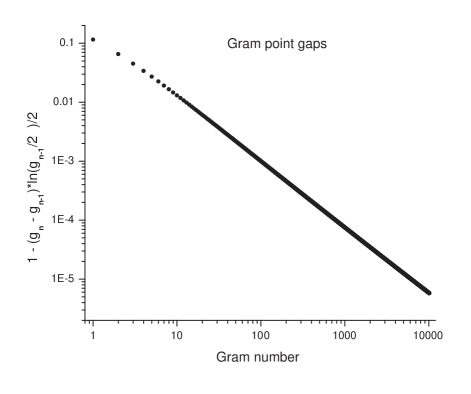
Figure 1: 1 minus the ratio between the actual gap between two consecutive Gram points and the large $n$ approximation of Eqn. (3), as a function of the Gram point number, $n$. Log-log plot.

There is a special subset of the Gram points which lie on contour lines Im$(\zeta(s))=0$, which run from $\sigma=~{}-\infty$ to $\sigma=~{}+\infty$ without passing through any zero of $\zeta(s)$.Arias03 ; Fisch12 These lines divide $\zeta(s)$ into strips which run roughly parallel to the real axis.

The contour lines Im$(\zeta(s))=0$ and Re$(\zeta(s))=0$ are highly constrained by the Cauchy-Riemann equations. An extensive discussion of their properties, including many illustrations, has been given by Arias de Reyna.Arias03 In the work presented here, the author used the computer program of Collins to study these lines.Col09 It is not practical to find double precision values for the locations of the Gram points directly from the output of Collins’ computer program. Finding approximate values from the graphical output of this program, the accurate values used for Fig. 1 were taken from a list supplied to the author by Michael Rubinstein.Rub13

As shown by Arias de Reyna,Arias03 two Im$(\zeta(s))=0$ contour lines which pass through special Gram points cannot intersect when $\sigma>1/2$. However, there is no general proof that contour lines of Im$(\zeta(s))=0$ cannot intersect, although no such intersections are known to exist. A proof of this would immediately imply that all the zeroes of $\zeta(s)$ are simple, an unsettled issue which has been of interest for a long time. If it is possible for two Im$(\zeta(s))=0$ contour lines to intersect, then the strips bounded by the contour lines running through the special Gram points might not be well defined.

In order for two of these Im$(\zeta(s))=0$ contour lines to intersect at a point $s^{*}$, two conditions must be satisfied simultaneously. The first condition is that $\zeta^{\prime}(s^{*})=0$, where $\zeta^{\prime}(s)$ is the derivative of $\zeta(s)$. The second condition is that Im$(\zeta(s^{*}))=0$. It is knownLM74 that the RH requires that there be no zeroes of $\zeta^{\prime}(s)$ for $\sigma<1/2$. Therefore, the strips are well defined if the RH is true and in addition all the zeroes of $\zeta(s)$ are simple.

In this work we will study the properties of the special Gram points and their associated contour lines. Using data up to a height $t=10^{4}$, we will find numerical evidence of some remarkable behavior which is a result of the way the smooth, monotonic variation in the spacings between neighboring Gram points, as illustrated in Fig. 1, fits together with the strips bounded by the Im$(\zeta(s))=0$ contour lines. The average width of these strips does not depend on the height $t$. The author suspects that this behavior is related in some way to Dyson’s conjectureDyson09 about the connection of the RH with quasicrystals.

II Numerical results

We define the Riemann-Siegel phase $\theta(s)$ by

$$\zeta(s)~{}=~{}|\zeta(s)|\exp(i\theta(s))\,.$$ (4)

Then the contour lines at the top and the bottom of each strip have $\cos(\theta)$ = 1, i.e. $\theta$ is an integer multiple of $2\pi$. Counting the crossings of the critical line, $s$ = 1/2, by these contour lines passing through the special Gram points, we plot the number of strips as a function of the height $t$ for the first 1102 strips in Fig. 2.

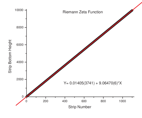
Figure 2: Height of the bottom of a strip on the critical line $\sigma$ = 1/2 as a function of strip number, $m$, for the first 1102 strips.

The linear least squares fit to the data is

$$Y~{}=~{}0.014(37)~{}+~{}9.06470(6)*X\,,$$ (5)

where the numbers in parentheses are the statistical errors in the last significant figure. Since there is a nontrivial distribution of strip widths, there is a small amount of jitter of the data around the fitting line. However, there is absolutely no indication of any curvature in the fit. The bottom of the first strip crosses the critical line at a height of $t$ = 9.6669080561 … . It is therefore somewhat mysterious that the Y-intercept of the fitting line is consistent (within the statistical error) with a value of zero. If one fits the heights of the tops of the strips instead, one finds (unsurprisingly) that the slope of the fitting line is essentially unchanged, but the Y-intercept is now found to be 9.07(5).

For large positive $\sigma$ Eqn. (1) can be approximated by its first two terms. Under this condition

$${\bf Im}(\zeta(s))~{}\approx~{}{\bf Im}(2^{-s})~{}=~{}2^{-\sigma}\sin(\ln(2)t)\,.$$ (6)

Thus the strip boundaries for large positive $\sigma$ and $t>0$ will be

$$t~{}\approx~{}2m\pi/\ln(2)\,,$$ (7)

where the strip number, $m$, is a positive integer. The numerical value of $2\pi/\ln(2)$ is 9.06472028… . Assuming the RH is correct, it seems a reasonable conjecture that the strips remain essentially horizontal for any value of $t$ when $\sigma>0$, which implies that the slope of the least squares fit for the heights of the bottom of each strip will be independent of $\sigma$. The author sees no reason, however, why the Y-intercept of this fit should be independent of $\sigma$. In fact, it appears that for $\sigma<0$ this Y-intercept becomes clearly greater than zero.

The reader should note that, since the sum on the right hand side of Eqn. (1) does not even converge for $\sigma=1/2$, it is rather surprising that the data taken on the critical line, shown in Fig. 2, are well fit by a straight line with a slope of $2\pi/\ln(2)$. Based on the analysis of Berry and Keating,BK99 for example, one might have expected to see oscillations about this line coming from the higher order terms of the sum. Somewhat similar ideas have been discussed by Steuding and Wegert.SW12

We now examine in detail the departures from the straight-line behavior, to see if there is anything resembling Berry-Keating oscillations. We do this by subtracting $2m\pi/\ln(2)$ from the actual height of the $m$-th special Gram point. The results for various ranges of $m$ up to 1102 are shown in Fig. 3 through Fig. 7.

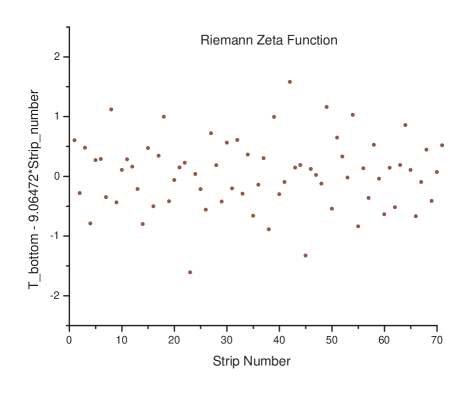
Figure 3: Deviation of the position of the $m$-th special Gram point from the average behavior, as a function of strip number, for the first 70 strips.

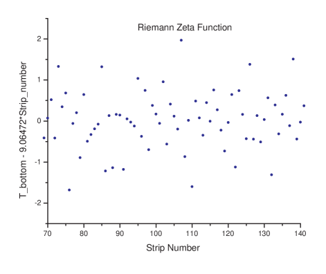
Figure 4: Deviation of the position of the $m$-th special Gram point from the average behavior, as a function of strip number, for strip numbers 70 to 140.

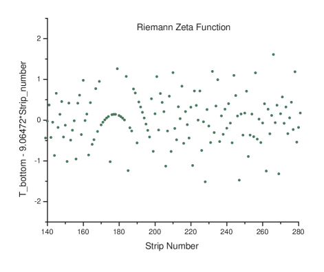
Figure 5: Deviation of the position of the $m$-th special Gram point from the average behavior, as a function of strip number, for strip numbers 140 to 280.

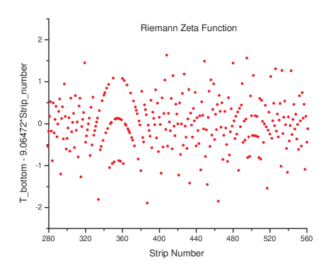
Figure 6: Deviation of the position of the $m$-th special Gram point from the average behavior, as a function of strip number, for strip numbers 280 to 560.

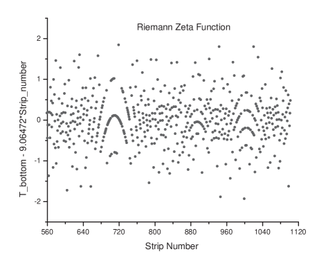
Figure 7: Deviation of the position of the $m$-th special Gram point from the average behavior, as a function of strip number, for strip numbers 560 to 1102.

Note that all of the points in the entire data set from 1 to 1102 have deviations in the range -2 to 2, and that the typical size of the deviations (i.e. the variance of the distribution of deviations) appears to be fairly insensitive to $m$. It is clear, however, that the points are not located randomly. There are obvious sets of nested arches which appear near certain values of $m$. This demonstrates rather extensive correlations exist in those regions where the arches are present.

It turns out that the heights where the nested arches appear are given by the simple expression

$$t_{\alpha}~{}=~{}2^{1+p/q}\pi\,,$$ (8)

where $p$ and $q$ are (positive) integers with no common prime factors. In units of the strip number, $m$, this expression has the form

$$\alpha(p,q)~{}=~{}2^{p/q}\ln(2)\,.$$ (9)

The most prominent arches in Figs. 3 to 7 are centered at locations given by $\alpha(p,1)$, for $p$ = 4, 5, 6, 7, 8, 9 and 10. Sets of secondary arches are found at values of $\alpha(p,2)$. In Fig. 6 and Fig. 7 there are also somewhat less defined arches which correspond to $q=3$ and perhaps $q=4$. The nested arches above and below the main arches are due to strips having one more or one less zero than they “ought” to have. Consistent with this idea, the vertical spacings between the nested arches for $q=2$ and $q=3$ are about 1/2 and 1/3, respectively, of the vertical spacings of the $q=1$ arches. In addition, all of these vertical spacings are decreasing slowly as $t$ increases.

For the $q=1$ case Eqn. (8) is obtained by requiring that $2\pi/\ln(2)$ divided by the spacing between consecutive Gram points at height $t$ be equal to $p$. This is a kind of resonance effect between the average height of a strip and the spacing between Gram points at height $t$. Similarly, the expression for larger values of $q$ may be thought of as higher order resonances.

It would, of course, be helpful to have an explicit analytical derivation of Eqn. (8). At this stage, we can only speculate about the behavior of these arches for very large values of the height $t$. It seems reasonable to guess that the $q=1$ and $q=2$ arches will continue to be present for large values of $t$. It is not clear to the author what will happen at large $t$ for larger values of $q$.

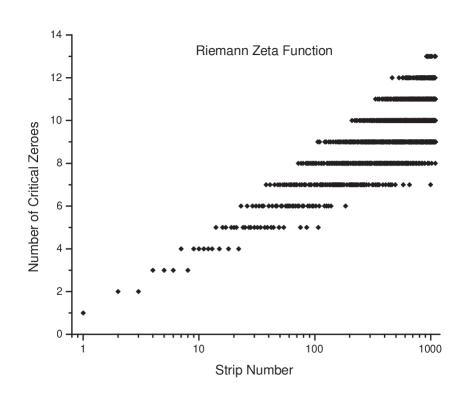
Figure 8: Number of critical zeroes in a strip versus strip number, for the first 1102 strips. The $X$-axis is scaled logarithmically.

The number of critical zeroes in a strip versus strip height is shown in Fig. 8. We see that the average number of zeroes increases logarithmically with strip number. It has been known for many years that the density of the critical zeroes increases approximately as $1/F(t)$, defined in Eqn. (3). The average density of critical zeroes as a function of $t$ is actually known to a much greater precision than this, because it is identical to the average density of Gram points. This follows directly from the fact that the RH and the assumption that all zeroes are simple implies that the number of zeroes in any strip must be equal to the number of Gram points, counting the special Gram point on the bottom edge but omitting the one on the top edge.

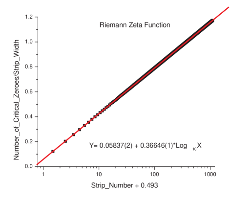
Figure 9: (Number of zeroes on the strip)/(strip width) versus strip number, for the first 1102 strips. The $X$-axis is scaled logarithmically.

Due to Eqn. (3) the width of each strip on the critical line $\sigma=1/2$ is determined to high accuracy by the height $t$ and the number of zeroes in the strip. In Fig. 9 we display the function (number of zeroes on the strip) divided by (strip width) versus the strip number. It is thus no surprise that these data lie on a straight line whose slope is determined by Eqn. 3, as shown in Fig. 9.

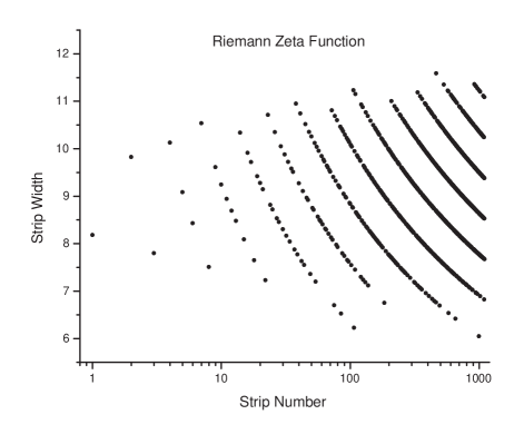
Figure 10: Strip width on the critical line $\sigma=1/2$ as a function of strip number, for the first 1102 strips. The $X$-axis is scaled logarithmically.

It is more revealing to plot the strip width versus strip number, shown in Fig. 10. We see that the data points sit close to lines which are hyperbolic. Each “line” contains all the points corresponding to a particular number of zeroes in a strip. The spacing between these lines is decreasing with $m$ logarithmically. There is an observable tendency for the range of strip widths to increase as $m$ increases, so it is not obvious what the large $m$ behavior will be.

In order to understand the behavior of the deviations of the points from the lines, we perform an analysis similar to the one of Figs. 3 to 7. In Fig. 11 to Fig. 15, we plot the deviations of the data from the straight line of Fig. 9. Note that the vertical scales of Figs. 11 to 15 are all different. The average deviation is decreasing approximately logarithmically as $m$ increases. This decrease compensates for the decrease in the spacing between the hyperbolic lines as the number of zeroes per strip increases. Therefore we expect that the qualitative behavior of Fig. 10, “lines” whose width is much narrower than the spacing between them, remains valid indefinitely as $m$ increases.

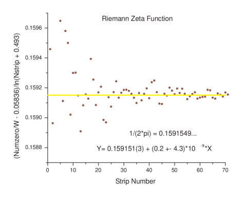
Figure 11: Deviation of the number of zeroes on strip $m$ divided by the width of strip $m$ from a straight line fit, as a function of strip number, for the first 70 strips.

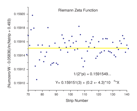
Figure 12: Deviation of the number of zeroes on strip $m$ divided by the width of strip $m$ from a straight line fit, as a function of strip number, for strip numbers 70 to 140.

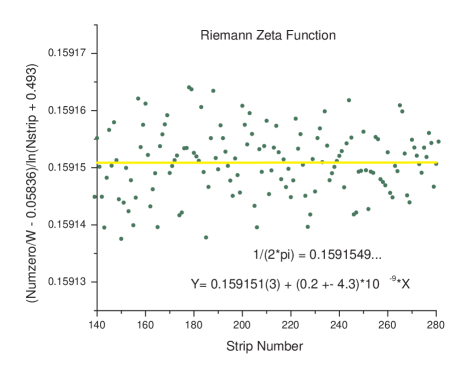
Figure 13: Deviation of the number of zeroes on strip $m$ divided by the width of strip $m$ from a straight line fit, as a function of strip number, for strip numbers 140 to 280.

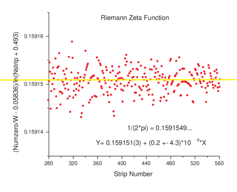
Figure 14: Deviation of the number of zeroes on strip $m$ divided by the width of strip $m$ from a straight line fit, as a function of strip number, for strip numbers 280 to 560.

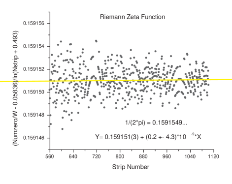
Figure 15: Deviation of the number of zeroes on strip $m$ divided by the width of strip $m$ from a straight line fit, as a function of strip number, for strip numbers 560 to 1102.

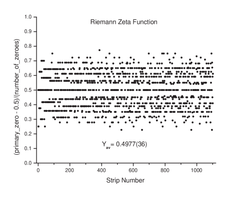
Figure 16: (Number of the primary zero $-~{}0.5$)/(Number of zeroes) versus strip number, for the first 1102 strips.

Due to the requirements of the Cauchy-Riemann equations, in each strip there is one special zero, which we will call the primary zero. Each primary zero has the property that the contour with phase $\theta$ = 0 going out of it extends to $\sigma~{}=~{}+\infty$, at a height

$$t~{}\approx~{}(2m+1)\pi/\ln(2)\,.$$ (10)

For all the other critical zeroes, the contour with phase $\theta~{}=~{}0$ goes to $\sigma~{}=~{}-\infty$.

One can now ask the question “Where is the primary zero located in the strip?” It seems obvious, by reason of symmetry, that the average position of the primary zero should be at the center of the strip. However, there is no symmetry reason why the probability distribution for the primary zero should be uniform. In Fig. 16 we display the values for the function (number of the primary zero (counting from the bottom of the strip) $-~{}0.5$) divided by (number of zeroes in the strip) versus the strip number. The subtraction of 0.5 in the numerator is necessary so that this function has the value 0.5 when the primary zero is the middle zero.

The linear least squares fit to the data of Fig. 16 shows that the average position of the primary zero is indeed at the center of the strip. Remarkably, one sees that the width of this probability distribution seems to be independent of the height. This observation is quantitatively confirmed by calculating the variance for subsets of the data, which always gives a result close to 0.014, independent of the range of $t$ used.

If this probability distribution remains nontrivial (i.e. neither becoming uniform nor collapsing) in the limit $t\to\infty$, then we must conclude that all of the zeroes in a strip are a collective entity, and that the positions of these zeroes are highly correlated with each other.

III Summary

In this work we have done an analysis of some properties of the special Gram points of the Riemann zeta function. We have uncovered some previously unknown facets of the behavior of this remarkable function along its critical line. The most remarkable of these occur when the ratio between $2\pi/\ln(2)$, the average strip width, and the spacing between Gram points passes through integers or rational numbers of small denominator. This seems to be some kind of a resonance effect, but its origin is not clear at this point.

- (1) The Riemann Hypothesis, edited by P. Borwein, S. Choi, B. Rooney and A. Weirathmueller (Springer, New York, 2008).
- (2) J. B. Conrey, Notices Amer. Math. Soc. 50, 341 (2003).
- (3) M. V. Berry and J. P. Keating, SIAM Rev. 41, 236 (1999).
- (4) G. Sierra and P. K. Townsend, Phys. Rev. Lett. 101, 110201 (2008).
- (5) R. Mack et al., Phys. Rev. A 82, 032119 (2010).
- (6) D. Shumayer and D. A. W. Hutchinson, Rev. Mod. Phys. 83, 307 (2011).
- (7) Y. V. Fyodorov, G. A. Hiary and J. P. Keating, Phys. Rev. Lett. 108, 170601 (2012).
- (8) H. M. Edwards, Riemann’s Zeta Function, (Academic Press, New York, 1974).
- (9) H. M. Edwards, op. cit., p. 126.
- (10) J. Arias de Reyna, arXiv:math/0309433v1 (2003).
- (11) R. Fisch, arXiv:1210.3618v1 (2012).
- (12) B. Collins, Contour Plots of the Zeta Function from the Wolfram Demonstrations Project, http://demonstrations.wolfram.com/ContourPlotsOfTheZetaFunction/ (2009). In manual mode, this program will accept decimal fractions as input values.
- (13) M. O. Rubinstein, unpublished.
- (14) N. Levinson and H. L. Montgomery, Acta Math. 133, 49 (1974).
- (15) F. J. Dyson, Notices Amer. Math. Soc. 56, 212 (2009).
- (16) J. Steuding and E. Wegert, Experimental Math. 21, 235 (2012).