Constraining the primordial power spectrum from SNIa lensing dispersion

Abstract

The (absence of detecting) lensing dispersion of supernovae type Ia (SNIa) can be used as a novel and extremely efficient probe of cosmology. In this preliminary example we analyze its consequences for the primordial power spectrum. The main setback is the knowledge of the power spectrum in the nonlinear regime, $1\,\mathrm{Mpc}^{-1}\lesssim k\lesssim 10^{2}-10^{3}\,\mathrm{Mpc}^{-1}$ up to redshift of about unity. By using the lensing dispersion and conservative estimates in this regime of wave numbers, we show how the current upper bound $\sigma_{\mu}(z\leq 1)<0.12$ on existing data gives strong indirect constraints on the primordial power spectrum. The probe extends our handle on the spectrum to a total of $12-15$ inflation e-folds. These constraints are so strong that they are already ruling out a large portion of the parameter space allowed by PLANCK for running, $\alpha\equiv dn_{s}/d\ln k$, and running of running, $\beta\equiv d^{2}n_{s}/d\ln k^{2}$. The bounds follow a linear relation to a very good accuracy. A conservative bound disfavors any enhancement above the line $\beta(k_{0})=0.036-0.42\,\alpha(k_{0})$ and a realistic estimate disfavors any enhancement above the line $\beta(k_{0})=0.022-0.44\,\alpha(k_{0})$.

Introduction: Cosmology is becoming a precise science, most notably due to increasing number and quality of measurements. Utilizing several probes is crucial in breaking degeneracies between cosmological parameters. The combination of CMB, large scale structure (LSS) and Type Ia Supernovae (SNIa) has lead to the emergence of the “concordance model” of cosmology. SNIa are widely used in cosmology due to their small intrinsic dispersion around their mean luminosity. By observing supernovae at cosmological distances, we can measure the luminosity-redshift relation $d_{L}(z)$ and infer cosmological parameters from the mean luminosity. However, the intrinsic dispersion of SNIa luminosities is not the only source of scatter in the data. Photons arriving from these ‘Standard Candles’ are affected by the inhomogeneous matter distribution between the source and observer. This induces an additional scatter in the luminosity-redshift relation, making it a stochastic observable with mean, dispersion, etc. Therefore, by disentangling this cosmic dispersion from the intrinsic scatter, we can potentially probe background parameters like $\Omega_{m0}$ or fluctuations, i.e. the power spectrum. Our main interest will be the lensing contribution, which dominates the cosmic dispersion at $z\gtrsim 0.3$.

We suggest using the lensing dispersion of SNIa as an additional probe of cosmology. The now operational Dark Energy Survey Bernstein et al. (2012) will measure thousands of SNIa, up to redshift $z\sim 1.2$ and LSST Abell et al. (2009) will measure millions of SNIa. This will reduce statistical errors considerably and increase the chance for detection since the lensing dispersion grows with the redshift at $z\sim 1$ Dodelson and Vallinotto (2006); Hui and Greene (2006); Ben-Dayan et al. (2013a). With future data, it has been suggested to use the lensing dispersion to constrain certain cosmological properties Hamana and Futamase (2000); Minty et al. (2002); Dodelson and Vallinotto (2006); Marra et al. (2013); Quartin et al. (2013).

In this preliminary paper we analyze the implications of the lensing dispersion $\sigma_{\mu}(z)$ on the primordial power spectrum. The distance modulus, $\mu=5\log_{10}({d_{L}(z)}/{\mathrm{10pc}})$, is a function of the luminosity distance $d_{L}(z)$ to the source at redshift $z$. Existing data analysis has not detected lensing dispersion with enough statistical significance, but has placed an upper bound of $\sigma_{\mu}(z\leq 1)\leq 0.12$ for the redshift of up to unity Jonsson et al. (2010) at $95\%$ C.L. and other analyses Kowalski et al. (2008); Conley et al. (2011); Kronborg et al. (2010) yield similar results. A Bayesian analysis was carried out in Karpenka et al. (2012), suggesting a very marginal detection of a lensing signal. Finally, in Betoule et al. (2014) the Joint Light-curve Analysis (JLA) compiled $740$ SNIa, reducing considerably systematic errors. For $z\lesssim 1$ The JLA analysis used mean value of Jonsson et al. (2010) $\sigma_{\mu}(z)=0.055z$ and added a “coherent dispersion” $\sigma_{coh.}$ to account for any other sources of intrinsic variations. The outcome is $\sigma_{coh.}=0.106\pm 0.006$. Moreover, there is a clear trend of $\sigma_{coh.}$ decreasing with redshift. Hence, the JLA analysis gives a model independent estimate of the total observed dispersion. Given that $\sigma_{total}(z)=\sqrt{\sigma_{\mu}(z)^{2}+\sigma_{coh.}^{2}}\leq 0.12$, we find that considering $\sigma_{\mu}(z\leq 1)\leq 0.12$ is a rather conservative upper bound, and we shall use this bound in our analysis.

In principle, the primordial power spectrum is not limited to a specific parametrization. In practice, it is typically parameterized as $P_{k}=A_{s}(k/k_{0})^{n_{s}(k_{0})-1}$, where $k_{0}$ is a suitable “pivot scale”. A common, more general form, is when the spectral index $n_{s}(k)$ is scale dependent, and then expanded around the pivot scale $k_{0}$,

$$n_{s}(k)=\displaystyle n_{s}(k_{0})+\displaystyle\frac{\alpha(k_{0})}{2}\ln\frac{k}{k_{0}}+\displaystyle\frac{\beta(k_{0})}{6}\ln^{2}\frac{k}{k_{0}}\,,$$ (1)

where $\alpha$ is typically dubbed the “running” of the spectral index, and $\beta$, the “running of running”. The best constraints on $\alpha,\beta$ with $k_{0}=0.05\,\mathrm{Mpc}^{-1},\,n_{s}(k_{0})\simeq 0.96$ are given by PLANCK Ade et al. (2013) and $\mathrm{Ly_{\alpha}}$ Zhao et al. (2012). These analyses are only probing the range $H_{0}\leq k\lesssim 1\,\mathrm{Mpc}^{-1}$. The lensing dispersion, $\sigma_{\mu}$ is sensitive to $0.01\lesssim k\lesssim 10^{2}-10^{3}\,\mathrm{Mpc}^{-1}$, thus giving access to $2-3$ more decades of the spectrum. Hence, $\sigma_{\mu}(z)$ is particularly sensitive to the quasi-linear and non-linear part of the spectrum. In terms of inflation, the direct measurement of $k\lesssim 1\,\mathrm{Mpc}^{-1}$ corresponds to about $8$ e-folds of inflation, leaving most of the power spectrum of $\sim 60$ e-folds out of reach . Therefore, even after PLANCK there is still an enormous space of inflationary models allowed. It is therefore of crucial importance to infer as much of the spectrum as possible for a better inflationary model selection. The lensing dispersion constrains additional $4-7$ e-folds, yielding a total of $12-15$ e-folds.

Other methods of probing the primordial spectrum include methods such as $\mathrm{Ly_{\alpha}}$ Zhao et al. (2012), the absence of primordial black holes and Ultracompact Minihalos Alabidi et al. (2013); Bringmann et al. (2012); Li et al. (2012), measuring spectral distortions of the CMB blackbody spectrum Chluba et al. (2012a, b); Chluba and Jeong (2013), galaxy weak lensing Miyatake et al. (2013), galaxy correlation functions Marin et al. (2013) and cluster number counts Chantavat et al. (2009). All of which have either different systematics, different $k$ range sensitivity, based on future data or some combination of the above. Albeit degenerate with other cosmological parameters, $\sigma_{\mu}$ surpasses these methods by actually cutting into the allowed parameter space allowed by PLANCK, using existing data only. In a separate publication Ben-Dayan (2014), we analyze the case, where the power spectrum takes a different “non-slow-roll” parametrization such as in cases analyzed in Chluba et al. (2012b).

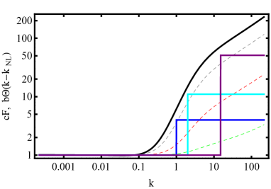
Figure 1: Log-Log plot of the “transfer functions” (5) at redshift $z=1$ multiplied by $c=1$ (solid black), $c=0.5$ (dashed grey), $c=0.1$ (dashed red) $c=0.01$ (dashed green). Solid blue, cyan and purple curves are the step functions in (6) with $b=3,k_{NL}=1\,\mathrm{Mpc}^{-1}$; $b=10,k_{NL}=2\,\mathrm{Mpc}^{-1}$; $b=50,k_{NL}=15\,\mathrm{Mpc}^{-1}$, respectively.

Method: We start from the full dispersion expression of the luminosity distance, calculated in the light-cone average approach up to second order in the Poisson (longitudinal) gauge, Gasperini et al. (2011); Ben-Dayan et al. (2012a, 2013b, b, 2013a), and recently confirmed in Fanizza et al. (2013). The dominant contribution of the dispersion at $z\gtrsim 0.3$, comes from the lensing contribution. For a perturbed FLRW Universe, one starts with the line of sight (LOS) first order lensing contribution to the distance modulus,

$$\delta\mu_{1}(\eta_{s}^{(0)})=\frac{5}{\ln 10}\int_{\eta_{s}^{(0)}}^{\eta_{o}}\frac{d\eta_{1}}{\Delta\eta}\frac{\eta_{1}-\eta_{s}^{(0)}}{\eta_{o}-\eta_{1}}\Delta_{2}\Psi\,,$$ (2)

where the gravitational potential $\Psi=\Psi(\eta_{i},r_{i},\tilde{\theta}^{a})$ is evaluated along the past light-cone at $r_{i}=\eta_{o}-\eta_{i}$, $\eta_{o}$ is the observer conformal time, $\eta_{s}^{(0)}$ is the conformal time of the source with unperturbed geometry, $\Delta\eta(z)=\eta_{o}(z)-\eta_{s}^{(0)}(z)=\int^{z}_{0}\frac{dy}{H_{0}\sqrt{\Omega_{m0}(1+y)^{3}+\Omega_{\Lambda 0}}}$ and $\Delta_{2}$ is the 2D angular Laplacian, see Ben-Dayan et al. (2013a, 2012a) for technical terms and explanations. Squaring (2) and taking the ensemble average in Fourier space at a fixed observed redshift, gives the variance, $\sigma^{2}_{\mu}(z)$ . In general, the calculation involves a complicated double line of sight (LOS) and wave number integration. However, at $z\gtrsim 0.3$, the double LOS integral is dominated by the equal time part, and further by $\mathrm{Si}(x\gg 1)\approx\pi/2$, yielding:

$$\sigma_{\mu}^{2} \simeq\left(\frac{5}{\ln 10}\right)^{2}\frac{\pi}{\Delta\eta^{2}}\int_{\eta_{s}^{(0)}}^{\eta_{o}}\frac{d\eta_{1}dk}{k}P_{\Psi}(k,\eta_{1})k^{3}$$ (3)

$$~{}~{}~{}~{}~{}~{}~{}~{}~{}~{}~{}~{}~{}~{}~{}~{}~{}~{}~{}~{}~{}~{}~{}~{}~{}~{}~{}~{}\times(\eta_{1}-\eta_{s}^{(0)})^{2}(\eta_{o}-\eta_{1})^{2}\,,$$

where $P_{\Psi}$ is the linear (LPS, $P_{L}$) or non-linear dimensionless power spectrum (NLPS, $P_{NL}$) of the gravitational potential . Hence, the lensing dispersion of supernovae is a direct measurement of the integrated late-time power spectrum. At the most basic level, this can be used to constrain parameterizations of $P_{\Psi}$, or cosmological parameters such as $\Omega_{m0},\sigma_{8}$ or $w(z)$. We will be mostly interested in the dispersion at $z=1$ where sufficient data is available and because up to the redshift of a few, the dispersion grows approximately linearly Holz and Linder (2005); Kronborg et al. (2010); Jonsson et al. (2010); Ben-Dayan et al. (2013a), so the best constraints can be given at the maximal available redshift. In general, the $k^{2}$ enhancement makes $\sigma_{\mu}$ a sensitive probe to the small scales of the power spectrum. To make this claim transparent, let us switch to dimensionless variables, $\tilde{\eta}=H_{0}\eta$ and $p=k/k_{eq}$ :

$$\sigma_{\mu}^{2}\simeq\left(\frac{5}{\ln 10}\right)^{2}\frac{\pi}{\Delta\tilde{\eta}^{2}}\left(\frac{k_{eq}}{H_{0}}\right)^{3}\int d\tilde{\eta}_{1}dpP_{\Psi}(p,\tilde{\eta}_{1})p^{2}$$ (4)

$$\times(\tilde{\eta}_{1}-\tilde{\eta}_{s}^{(0)})^{2}(\tilde{\eta}_{o}-\tilde{\eta}_{1})^{2}\,.$$

From this expression we learn that: $(a)$ The relevant physical scales are $H_{0}$ and $k_{eq}$, which give an enhancement of $(k_{eq}/H_{0})^{3}$. $(b)$ The dispersion is really sensitive to the scales smaller than the equality scale $p>1$. $(c)$ The NLPS has an additional redshift dependent physical scale which is the onset of nonlinearity. For a given redshift, parameterizing the NLPS as $\sim C(k/k_{NL})^{\nu}$, from some $k_{NL}$, will have an additional parametric enhancement of $(k_{NL}/k_{eq})^{3}$.

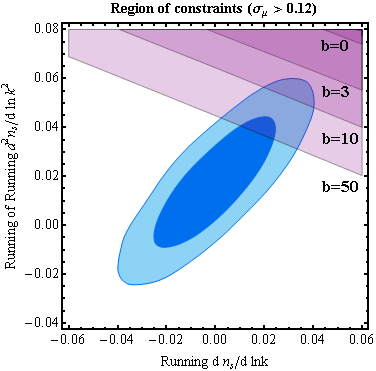
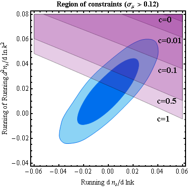
Figure 2: Regions of allowed parameters combined with PLANCK data. The ellipses are the 68% and 95% C.L. contours from Ade et al. (2013). In the colored regions $\sigma_{\mu}(z=1)>0.12$ and are disfavored for $b=0,1,3,10,50$ (left panel) and $c=0,0.01,0.1,0.5,1$ (right panel)

Equation (4) is free of IR and UV divergences so the main limitation is the validity of the spectrum Ben-Dayan et al. (2013a). For $k\gg H_{0}$ at some redshift dependent point standard cosmological perturbation theory breaks down, and one has to resort to numerical simulations to get an approximate fitting formula for the power spectrum. We use the HaloFit model Smith et al. (2003); Takahashi et al. (2012); Inoue and Takahashi (2012) with $k_{UV}=320h\,\mathrm{Mpc}^{-1}$. We have verified that varying $k_{UV}\in(30h,\infty)\,\mathrm{Mpc}^{-1}$ or $H_{0}$ and $\Omega_{m0}$ independently within the range $H_{0}\in[64,70]$, $\Omega_{m0}\in[0.27,0.36]$ gives at most $15\%$ change in the value of $\sigma_{\mu}$. Taken that $\sigma_{\mu}(z=1,\alpha=\beta=0,k_{UV}=320h\,\mathrm{Mpc}^{-1})=0.08$, the bound cannot be saturated by varying the background parameters and/or integrating up to arbitrarily small scales. Hence the bound can be useful for constraining $\alpha(k_{0})$ and $\beta(k_{0})$ and our results are accurate to about $20\%$.

Considering a big enough $\alpha$ and $\beta$, the HaloFit fitting formula is not reliable anymore due to its sensitivity to initial conditions. For example, with $\alpha=0.04$ and $\beta=0.05$ the existing HaloFit actually gives enhancement of a few at $1<k<175\,\,\mathrm{Mpc}^{-1}$ and a suppressed power spectrum compared to the linear one at larger $k$. It is nevertheless obvious that the non-linear evolution causes clustering and enhances the power spectrum. For example, at redshift $z=1$, the ratio between the HaloFit formula, $P_{NL}(k,z)$, with standard initial conditions $(n_{s}\simeq 0.96,\,\alpha=\beta=0)$ and the linear power spectrum $P_{NL}(k,1)/P_{L}(k,1)$ is the solid, thick, black curve plotted in Fig. 1. Already at $k=1\,\mathrm{Mpc}^{-1}$ the non-linear power spectrum is a factor of a few larger than the linear one, and for $k\gtrsim 10\,\mathrm{Mpc}^{-1}$, it behaves as a power law with a scaling exponent of nearly $1/2$. We therefore utilize this ratio in the standard case of $n_{s}=const.$ to define a “transfer function”,

$$F(k,z) \equiv \frac{P_{NL}(k,z)}{P_{L}(k,z)}\,,$$ (5)

where $P_{NL}$ is the non-linear power spectrum, $P_{L}=(3/5)^{2}P_{k}T^{2}(k)g^{2}(z)$ is the linear spectrum and $T(k)$ is the transfer function with baryons Eisenstein and Hu (1998), all taken in the standard scenario with $n_{s}\simeq 0.96,\alpha=\beta=0$. We take the enhancement into account in two simple ways. The first method is by the Heaviside function $\Theta(k)$. Here we are not limited to the HaloFit formula, so we perform the following substitution in equation (3),

$$P_{\Psi}\rightarrow P_{L}(k,z)(1+b\,\Theta(k-k_{NL}))$$ (6)

and we evaluate $\sigma_{\mu}$ for $b=0,3,10,50$ with corresponding $k_{NL}=1,1,2,15\,\mathrm{Mpc}^{-1}$, such that the step function is always underestimating the transfer function $F$, so this is a very conservative estimate. The step functions are the solid blue, cyan and purple lines in Fig. 1. The second method is to use $F$ of the HaloFit model, such that

$$P_{\Psi}\rightarrow P_{L}(k,z)(1-c+cF(k,z))\,,$$ (7)

and evaluate $\sigma_{\mu}$ with $c=0,0.01,0.1,0.5,1$. In both methods $b=0$ or $c=0$ correspond to computing the dispersion with the linear power spectrum only, while $c=1$ corresponds to exactly following the HaloFit enhancement pattern. Except $c=1$ all the second method values of $c$ are underestimates as well. The resulting enhancement at $z=1$, is plotted in Fig. 1 as green, red and grey dashed lines.

Results: In Fig. 2 we show the constraints on running and running of running from the non-detection of lensing dispersion overlaid on PLANCK likelihood contours. In the left panel, the values $b=0,3,10,50$ with corresponding $k_{NL}=1,1,2,15\,\mathrm{Mpc}^{-1}$ are considered. The right panel considers $c=0,0.01,0.1,0.5,1$. In both panels, colored regions give $\sigma_{\mu}(z=1)\geq 0.12$ and are disfavored.

We wish to note that there are additional factors which make our analysis an underestimate. First of all, partial sky coverage is expected to increase dispersion Hui and Greene (2006). Second, SNIa at higher redshift have already been detected and used for cosmological parameter inference. The monotonicity of $\sigma_{\mu}(z)$ ensures that considering, for instance, $\sigma_{\mu}(z=1.2)$ would give more stringent bounds. Third, the consideration of other analyses. Bayesian analyses March et al. (2011); Karpenka et al. (2012) suggested that the total dispersion is about $0.12$ with a very marginal detection of the lensing signal. Better yet, the JLA Betoule et al. (2014) is an up to date, model independent analysis and also there $\sigma_{total}(z\leq 1)\leq 0.12$, not just the lensing dispersion. In the above cases, the intrinsic or “coherent” dispersion, actually dominates the total dispersion. On top of that, in the JLA analysis there is a clear trend of $\sigma_{coh.}$ decreasing in redshift, meaning that the actual value of the lensing dispersion is probably smaller than the $\sigma_{\mu}=0.055z$ it uses. Last, all other analyses (data, statistical, theoretical and numerical) Kronborg et al. (2010); Jonsson et al. (2010); Ben-Dayan et al. (2013a); Holz and Linder (2005); Smith et al. (2013) point to a lower value of the dispersion as well, at most $\sigma_{\mu}(z)\simeq 0.093z$, practically disfavouring even a larger portion of the parameter space allowed by PLANCK.

Conclusions and Outlook: From Fig. 2, it is obvious that the lensing dispersion or its absence is an extremely powerful cosmological probe. Even if a scale dependent spectral index induces clustering which is an order of magnitude smaller than the standard constant $n_{s}$ scenario, some of the parameter space allowed by PLANCK is ruled out. Moreover, the analysis discusses the spectrum up to $k\sim 320h\,\mathrm{Mpc}^{-1}$, more than two orders of magnitude beyond PLANCK’s lever arm ($\sim 5$ e-folds more) irrespective of whether models are ruled in or out. It can be treated as a prediction of inflationary models. In the more realistic case where the enhancement is similar to the HaloFit model, such as $c=0.5,1$, one gets strong bounds on the allowed parameters, that can be expressed as a linear relation,

$$\beta(k_{0})\leq 0.036-0.42\,\alpha(k_{0}),\quad c=0.5$$ (8)

$$\beta(k_{0})\leq 0.022-0.44\,\alpha(k_{0}),\quad c=1.$$ (9)

The realistic case of $\beta(k_{0})\leq 0.022$ nicely matches PLANCK’s $\alpha(k_{0})=0^{+0.016}_{-0.013}\,,\beta(k_{0})=0.017_{-0.014}^{+0.016}$. Obviously, a definite detection of lensing will enable a more stringent analysis similar to CMB lensing.

It is very appealing to add the lensing dispersion constraint to the likelihood analysis of the PLANCK data. We believe that numerical simulations with initial conditions as suggested here, $\alpha(k_{0}),\beta(k_{0})\neq 0$, which will give a more accurate late time power spectrum, will yield similar results, thus strengthening our argument. These simulations are already on their way. Last, we have suggested using the (absence of) dispersion to constrain the primordial power spectrum. Since the dispersion depends on several cosmological parameters, it can be useful in constraining other fundamental cosmological parameters as well.

Acknowledgements It is a pleasure to thank Matthias Bartelmann, Torsten Bringmann, Jens Chluba, Thomas Konstandin, Alexander Westphal and Mathias Zaldarriaga for helpful discussions, comments and suggestions. The work of I.B.-D. is supported by the German Science Foundation (DFG) within the Collaborative Research Center (CRC) 676 Particles, Strings and the Early Universe. The work of T.K. was supported in part by the U.S. Department of Energy under Contract DE-FG-88ER40388.

References

- Bernstein et al. (2012) J. Bernstein, R. Kessler, S. Kuhlmann, R. Biswas, E. Kovacs, et al., Astrophys.J. 753, 152 (2012).
- Abell et al. (2009) P. A. Abell et al. (LSST Science Collaborations, LSST Project) (2009), eprint 0912.0201.
- Dodelson and Vallinotto (2006) S. Dodelson and A. Vallinotto, Phys.Rev. D74, 063515 (2006).
- Hui and Greene (2006) L. Hui and P. B. Greene, Phys.Rev. D73, 123526 (2006).
- Ben-Dayan et al. (2013a) I. Ben-Dayan, M. Gasperini, G. Marozzi, F. Nugier, and G. Veneziano, JCAP 1306, 002 (2013a).
- Hamana and Futamase (2000) T. Hamana and T. Futamase, ApJ 534, 29 (2000).
- Minty et al. (2002) E. M. Minty, A. F. Heavens, and M. R. Hawkins, Mon.Not.Roy.Astron.Soc. 330, 378 (2002).
- Marra et al. (2013) V. Marra, M. Quartin, and L. Amendola, Phys. Rev. D88, 063004 (2013).
- Quartin et al. (2013) M. Quartin, V. Marra, and L. Amendola (2013), eprint 1307.1155.
- Jonsson et al. (2010) J. Jonsson, M. Sullivan, I. Hook, S. Basa, R. Carlberg, et al., MNRAS 405, 535 (2010), eprint 1002.1374.
- Kowalski et al. (2008) M. Kowalski et al. (Supernova Cosmology Project), Astrophys.J. 686, 749 (2008).
- Conley et al. (2011) A. Conley, J. Guy, M. Sullivan, N. Regnault, P. Astier, et al., Astrophys.J.Suppl. 192, 1 (2011).
- Kronborg et al. (2010) T. Kronborg, D. Hardin, J. Guy, P. Astier, C. Balland, et al. (2010), eprint 1002.1249.
- Karpenka et al. (2012) N. Karpenka, M. March, F. Feroz, and M. Hobson (2012), eprint 1207.3708.
- Betoule et al. (2014) M. Betoule et al. (SDSS Collaboration), Astron.Astrophys. (2014), eprint 1401.4064.
- Ade et al. (2013) P. Ade et al. (Planck Collaboration) (2013), eprint 1303.5082.
- Zhao et al. (2012) G.-B. Zhao, S. Saito, W. J. Percival, A. J. Ross, F. Montesano, et al. (2012), eprint 1211.3741.
- Alabidi et al. (2013) L. Alabidi, K. Kohri, M. Sasaki, and Y. Sendouda, JCAP 1305, 033 (2013).
- Bringmann et al. (2012) T. Bringmann, P. Scott, and Y. Akrami, Phys.Rev. D85, 125027 (2012).
- Li et al. (2012) F. Li, A. L. Erickcek, and N. M. Law, Phys.Rev. D86, 043519 (2012).
- Chluba et al. (2012a) J. Chluba, R. Khatri, and R. A. Sunyaev (2012a), eprint 1202.0057.
- Chluba et al. (2012b) J. Chluba, A. L. Erickcek, and I. Ben-Dayan, Astrophys.J. 758, 76 (2012b).
- Chluba and Jeong (2013) J. Chluba and D. Jeong (2013), eprint 1306.5751.
- Miyatake et al. (2013) H. Miyatake, S. More, R. Mandelbaum, M. Takada, D. N. Spergel, et al. (2013), eprint 1311.1480.
- Marin et al. (2013) F. A. Marin et al. (WiggleZ Collaboration) (2013), eprint 1303.6644.
- Chantavat et al. (2009) T. Chantavat, C. Gordon, and J. Silk, Phys.Rev. D79, 083508 (2009), eprint 0811.4371.
- Ben-Dayan (2014) I. Ben-Dayan (2014), eprint 1408.3004.
- Gasperini et al. (2011) M. Gasperini, G. Marozzi, F. Nugier, and G. Veneziano, JCAP 1107, 008 (2011).
- Ben-Dayan et al. (2012a) I. Ben-Dayan, M. Gasperini, G. Marozzi, F. Nugier, and G. Veneziano, JCAP 1204, 036 (2012a).
- Ben-Dayan et al. (2013b) I. Ben-Dayan, M. Gasperini, G. Marozzi, F. Nugier, and G. Veneziano, Phys.Rev.Lett. 110, 021301 (2013b).
- Ben-Dayan et al. (2012b) I. Ben-Dayan, G. Marozzi, F. Nugier, and G. Veneziano, JCAP 1211, 045 (2012b).
- Fanizza et al. (2013) G. Fanizza, M. Gasperini, G. Marozzi, and G. Veneziano (2013), eprint 1308.4935.
- Holz and Linder (2005) D. E. Holz and E. V. Linder, Astrophys.J. 631, 678 (2005).
- Smith et al. (2003) R. Smith et al. (Virgo Consortium), Mon.Not.Roy.Astron.Soc. 341, 1311 (2003).
- Takahashi et al. (2012) R. Takahashi, M. Sato, T. Nishimichi, A. Taruya, and M. Oguri, Astrophys.J. 761, 152 (2012).
- Inoue and Takahashi (2012) K. T. Inoue and R. Takahashi, Mon.Not.Roy.Astron.Soc. 426, 2978 (2012).
- Eisenstein and Hu (1998) D. J. Eisenstein and W. Hu, ApJ 496, 605 (1998).
- March et al. (2011) M. March, R. Trotta, P. Berkes, G. Starkman, and P. Vaudrevange, Mon.Not.Roy.Astron.Soc. 418, 2308 (2011), eprint 1102.3237.
- Smith et al. (2013) M. Smith et al. (SDSS Collaboration), Astrophys.J. (2013), eprint 1307.2566.