A scan of f(R) models admitting Rindler type acceleration

Abstract

As a manifestation of large distance effect Grumiller modified Schwarzschild metric with an extraneous term reminiscent of Rindler acceleration. Such a term has the potential to explain the observed flat rotation curves in general relativity. The same idea has been extended herein to the larger arena of $f\left(R\right)$ theory. With particular emphasis on weak energy conditions (WECs) for a fluid we present various classes of $f\left(R\right)$ theories admitting a Rindler-type acceleration in the metric.

I INTRODUCTION

Flat rotation curves around galaxies constitute one of the most stunning astrophysical findings since 1930s. The cases can simply be attributed to the unobservable dark matter which still lacks a satisfactory candidate. On the general relativity side which reigns in the large universe an interesting approach is to develop appropriate models of constant centrifugal force. One such attempt was formulated by Grumiller 1 ; 2 in which the centrifugal force was given by $F=-\left(\frac{m}{r^{2}}+a\right)$. Here $m$ represents the mass (both normal and dark) while the parameter ”$a$” is a positive constant - called Rindler acceleration 3 - which gives rise to a constant attractive force. The Newtonian potential involved herein is $\Phi\left(r\right)\sim-\frac{m}{r}+ar$ , so that for $r\rightarrow\infty$ the term $\Phi\left(r\right)\sim ar$ becomes dominant. Since in Newtonian circular motion $F=\frac{mv^{2}}{r}$, for a mass $m,$ tangential speed $v\left(r\right)$ and radius $r$ are related by $v\left(r\right)\sim r^{\frac{1}{2}}$ for large $r$, overall which amounts slightly nearer to the concept of flat rotation curves. No doubts, the details and exact flat rotation curves must be much more complicated than the toy model depicted here. Physically the parameter ”$a$” becomes meaningful when one refers to an accelerated frame in a flat space, known as Rindler frame and accordingly the terminology Rindler acceleration is adopted.

In 4 impact of a Rindler-type acceleration is studied on the Oort Cloud and in 5 the solar system constraints on Rindler acceleration is investigated while in 6 bending of light in the model of gravity at large distances proposed by Grumiller 1 ; 2 is considered.

Let us add also that to tackle the flat rotation curves, Modified Newtonian Dynamics (MOND) in space was proposed 7 . Assuming a physical source to the Rindler acceleration term in the spacetime metric has been challenging in recent years. Anisotropic fluid field was considered originally by Grumiller 1 ; 2 , whereas nonlinear electromagnetism was proposed as an alternative source 8 . A fluid model with energy-momentum tensor of the form $T_{\mu}^{\nu}=diag[-\rho,p,q,q]$ was proposed recently in the popular $f\left(R\right)$ gravity 9 . For a review of the latter we propose 10 ; 11 ; 12 . By a similar strategy we wish to employ the vast richness of $f(R)$ gravity models to identity possible candidates that may admit Rindler type acceleration. Our approach in this study beside the Rindler acceleration is to elaborate on the energy conditions in $f\left(R\right)$ gravity. Although violation of the energy conditions is not necessarily a problem (for instance, any quantum field theory violates all energy conditions) but it is still interesting to investigate the non-violation of the energy conditions. Note that energy conditions within the context of dark matter in $f(R)$ gravity was considered by various authors 13 . This at least will filter the viable models that satisfy the energy conditions. In brief, for our choice of energy-momentum the weak energy conditions (WECs) can be stated as follow: i) WEC1 says that energy density $\rho\geqslant 0$. ii) WEC2, says that $\rho+p\geqslant 0$, and iii) WEC3 states that $\rho+q\geqslant 0$. The more stringent energy conditions, the strong energy conditions (SECs) amounts further to $\rho+p+2q\geqslant 0$, which will not be our concern in this paper. However, some of our models satisfy SECs as well. Our technical method can be summarized as follows. Upon obtaining $\rho,$ $p$ and $q$ as functions of $r$ we shall search numerically for the geometrical regions in which the WECs are satisfied. (A detailed work on energy condition in $f(R)$ gravity was done by J. Santos et al in 14 ).

From the outset our strategy is to assume validity of the Rindler modified Schwarzschild metric a priori and search for the types of $f(R)$ models which are capable to yield such a metric. Overall we test ten different models of $f\left(R\right)$ gravity models and observe that in most cases it is possible to tune free parameters in rendering the WECs satisfied. In doing this we entirely rely on numerical plots and we admit that our list is not an exhaustive one in $f\left(R\right)$ arena.

Organization of the paper goes as follows. Sec. II introduces the formalism with derivation of density and pressure components. Sec. III presents eleven types of $f\left(R\right)$ models relevant to the Mannheim’s metric. The paper ends with Conclusion in Sec. IV.

II The Formalism

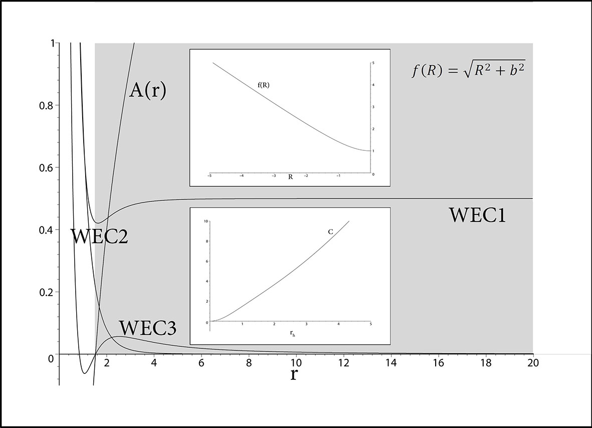
Figure 1: A plot of $WEC1,$ $WEC2$ and $WEC3$ for $m=1$, $a=0.1$ and $b=1.$ To have an idea of the range in which WECs are satisfied we also plot the metric function which identifies the location of the horizon. It is observed from the figure that WECs are all satisfied for $r\geq r_{h}$ in which $r_{h}$ is the event horizon of the Grumiller’s metric. Since $R<0$ the plot of $f(R)$ is from $-\infty$ up to zero and as can be seen $\frac{df}{dR}<0$ while $\frac{d^{2}f}{dR^{2}}>0$. We also plot the heat capacity $C$ w.r.t the horizon radius $r_{h}$.

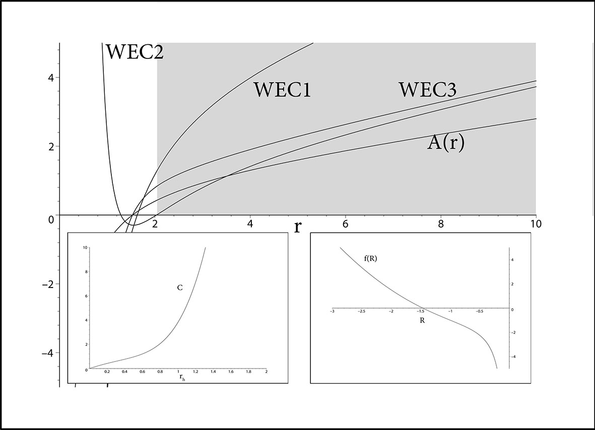
Figure 2: Our choice of the parameters are $\nu=1,$ $\mu=2,$ $b=1,$ $c=-1,$ $\Lambda_{1}=0=\Lambda_{2}$. WECs are shown to satisfy while stability is valid only for $R<-1$. This can easily be checked from $f\left(R\right)=R+\frac{1}{R}+R^{2}.$ Thermodynamic stability (i.e. $C>0$) is also shown in the inscription.

Let’s start with the following action ($\kappa=8\pi G=1$)

$$S=\frac{1}{2}\int\sqrt{-g}f\left(R\right)d^{4}x+S_{M}$$ (1)

where $f\left(R\right)$ is a function of the Ricci scalar $R$ and $S_{M}$ is the physical source for a perfect fluid-type energy momentum

$$T_{\mu}^{\nu}=\left(\begin{array}[]{cccc}-\rho&0&0&0\\ 0&p&0&0\\ 0&0&q&0\\ 0&0&0&q\end{array}\right)$$ (2)

We adopt the static spherically symmetric line element

$$ds^{2}=-A\left(r\right)dt^{2}+\frac{1}{A(r)}dr^{2}+r^{2}\left(d\theta^{2}+\sin^{2}\theta d\varphi^{2}\right)$$ (3)

with

$$A\left(r\right)=1-\frac{2m}{r}+2ar$$ (4)

which will be referred henceforth as the Mannheim’s metric 15 (Note that it has been rediscovered by Grumiller in 1 ; 2 ). Einstein’s field equations follow the variation of the action with respect to $g_{\mu\nu}$ which reads as

$$G_{\mu}^{\nu}=\frac{1}{F}T_{\mu}^{\nu}+\check{T}_{\mu}^{\nu}$$ (5)

in which $G_{\mu}^{\nu}$ is the Einstein’s tensor. The share of the curvature in the energy-momentum is given by

$$\check{T}_{\mu}^{\nu}=\frac{1}{F}\left[\nabla^{\nu}\nabla_{\mu}F-\left(\square F-\frac{1}{2}f+\frac{1}{2}RF\right)\delta_{\mu}^{\nu}\right]$$ (6)

while $T_{\mu}^{\nu}$ refers to the fluid source 1 ; 2 . Following the standard notation, $\square=\nabla^{\mu}\nabla_{\mu}=\frac{1}{\sqrt{-g}}\partial_{\mu}\left(\sqrt{-g}\partial^{\mu}\right)$ and $\nabla^{\nu}\nabla_{\mu}u=g^{\lambda\nu}\nabla_{\lambda}u_{,\mu}=g^{\lambda\nu}\left(\partial_{\lambda}u_{,\mu}-\Gamma_{\lambda\mu}^{\beta}u_{,\beta}\right)$ for a scalar function $u$. The three independent Einstein’s field equations are explicitly given by

$$FR_{t}^{t}-\frac{f}{2}+\square F=\nabla^{t}\nabla_{t}F+T_{t}^{t}$$ (7)

$$FR_{r}^{r}-\frac{f}{2}+\square F=\nabla^{r}\nabla_{r}F+T_{r}^{r}$$ (8)

$$FR_{\theta_{i}}^{\theta_{i}}-\frac{f}{2}+\square F = \nabla^{\theta_{i}}\nabla_{\theta_{i}}F+T_{\theta_{i}}^{\theta_{i}}$$ (10)

$$\left(F=\frac{df}{dR}\right),$$

in which $\theta_{i}=\left(\theta,\varphi\right).$ Adding these equations (i.e., $tt$, $rr$, $\theta\theta$ and $\varphi\varphi$) one gets the trace equation

$$FR-2f+3\square F=T$$ (11)

which is not an independent equation. Using the field equations one finds

$$\rho=\nabla^{t}\nabla_{t}F-FR_{t}^{t}+\frac{f}{2}-\square F,$$ (12)

$$p=-\nabla^{r}\nabla_{r}F+FR_{t}^{t}-\frac{f}{2}+\square F,$$ (13)

and

$$q=-\nabla^{\theta}\nabla_{\theta}F+FR_{\theta}^{\theta}-\frac{f}{2}+\square F.$$ (14)

In what follows we find the energy momentum components for different models of $f(R)$ gravity together with their thermodynamical properties.

III $f(R)$ Models apt for the Rindler Acceleration

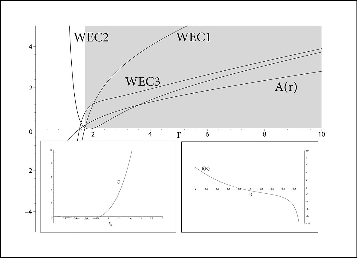
Figure 3: Our parameters in this case are $\nu=1,$ $\mu=2,$ $b=-1,$ $c=-1$ with $\Lambda_{1}=0=\Lambda_{2}$. So that $f(R)$ takes the form $f\left(R\right)=R+\frac{1}{R}-R^{3}$ which satisfies the WECs. This choice yields a stable model for $R<-\frac{1}{\sqrt[4]{3}}.$ Beyond certain horizon radius the specific function $C$ is also positive.

In this section we investigate a set of possible $f(R)$ gravity models which admit the line element (3) as the static spherically symmetric solution of its field equations. Then by employing Eq.s (12) to (14) we shall find the energy density $\rho$ and the pressures $p$ and $q.$ Having found $\rho$, $p$ and $q$ we investigate the energy conditions together with the feasibility of the $f(R)$ models numerically. More precisely we work on weak energy conditions which includes three individual conditions

$$WEC1=\rho\geq 0,$$ (15)

$$WEC2=\rho+q\geq 0$$ (16)

and

$$WEC3=\rho+p\geq 0.$$ (17)

In the numerical plotting, we plot explicitly $WEC1,$ $WEC2$ and $WEC3$ in terms of $r$ to work out the region(s) in which the WECs are satisfied. In addition to WECs we plot $f\left(R\right)$ in terms of $R$ to find out the physically acceptable model by imposing the well known conditions on $f\left(R\right)$ which are given by

$$F\left(R\right)=\frac{df\left(R\right)}{dR}>0$$ (18)

for not to have ghost field and

$$\frac{d^{2}f\left(R\right)}{dR^{2}}>0$$ (19)

to have a stable model. Before we start to study the $f(R)$ models, we add that in the case of Mannheim’s metric the Ricci scalar is given by $R=-\frac{12a}{r}$ which is negative ($a>0$).

III.1 The Models

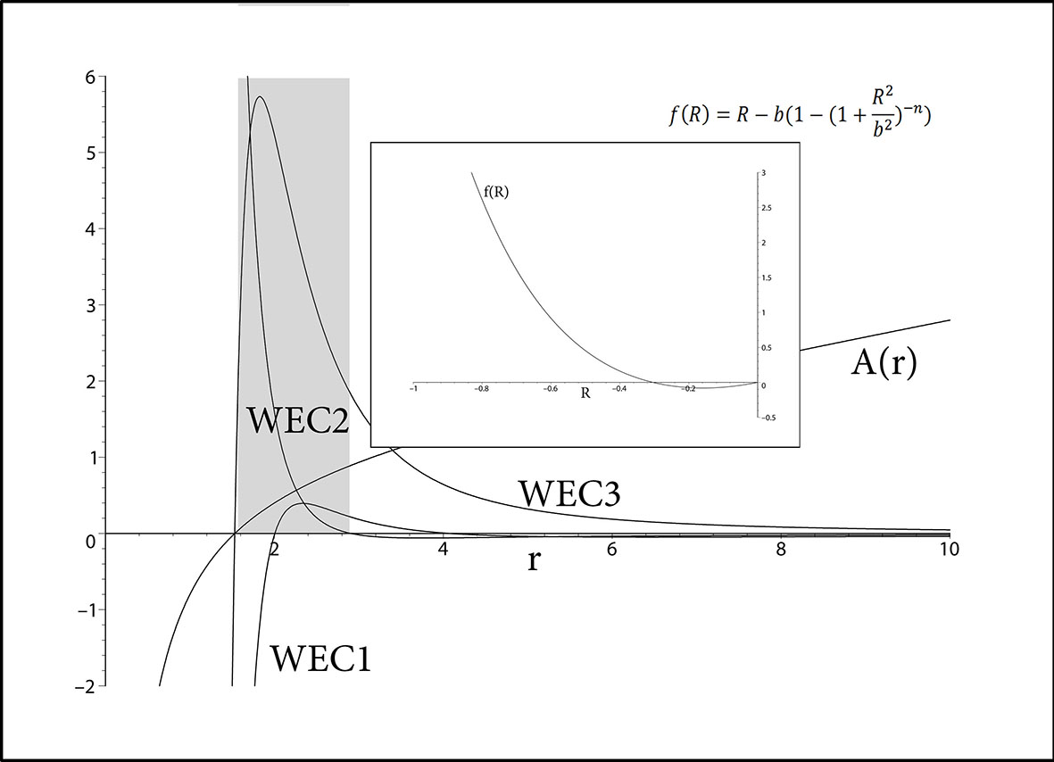
Figure 4: From Eq. (31) we choose the parameters as $\mu=1,$ $b=1$ and $n=-3$. We find a restricted domain in which WECs are satisfied. From those parameters beside WECs from $\frac{d^{2}f}{dR^{2}}=6\left(1+R^{2}\right)\left(1+5R^{2}\right)>0$ the stability condition also is satisfied.

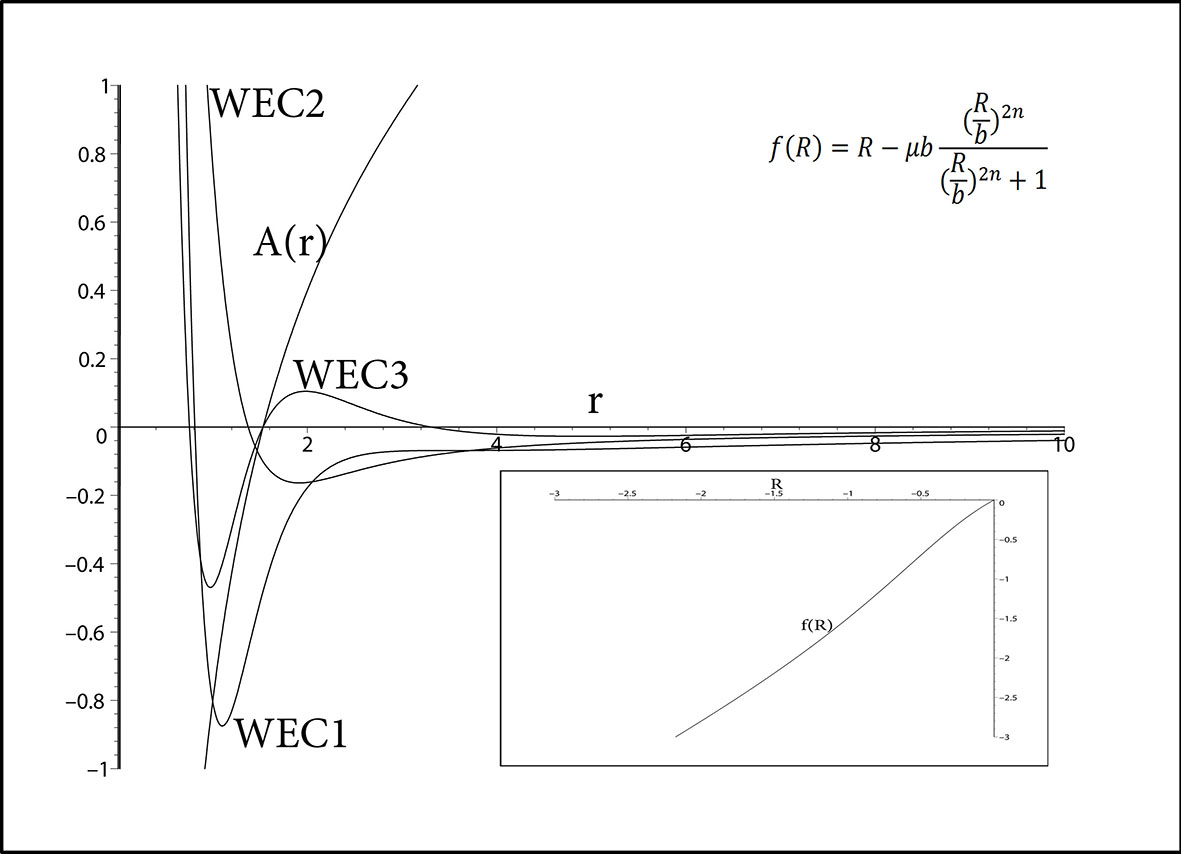
Figure 5: In this model given by the $f(R)$ in Eq. (32) we have not been able to find a physically admissible region to satisfy WECs.

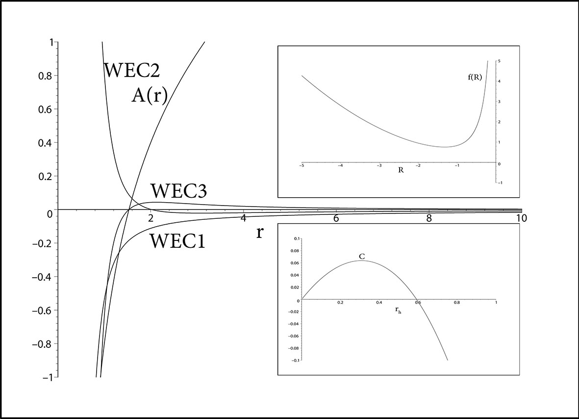
Figure 6: From $f\left(R\right)$ model in Eq. (33) the choice $c=1/3,$ $\varepsilon=1$ and $b=1$ , we observe that WECs are not satisfied. Specific heat function is also pictured in the inscription.

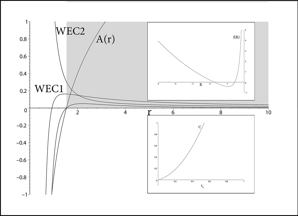
Figure 7: The choice of parameters $c=1.1,$ $\varepsilon=1$ and $b=1$ in Eq. (33) yields a region where WECs are satisfied. It can be checked that $\frac{d^{2}f}{dR^{2}}>0$ is also satisfied. For $\left|R\right|>\left|R_{0}\right|$ where $f^{\prime}\left(R_{0}\right)=0,$ $\frac{df}{dR}>0$ which implies ghost free solution. Everywhere positive specific heat $C$ is also shown in the inscription.

1) Our first model which we find interesting is given by 16

$$f\left(R\right)=\sqrt{R^{2}+b^{2}}$$ (20)

for $b=$constant. For $\left|R\right|\gg b,$ this model is a good approximation to Einstein’s $f(R)=R$ gravity. For the other extent, namely $\left|R\right|\ll b$, $b$ may be considered as a cosmological constant. Having this $f\left(R\right)$ one finds

$$\frac{df}{dR}=\frac{R}{\sqrt{R^{2}+b^{2}}}$$ (21)

$$\frac{d^{2}f}{dR^{2}}=\frac{b^{2}}{\left(R^{2}+b^{2}\right)^{3/2}}$$ (22)

which are positive functions with respect to $R$. This means that this model of $f(R)$ gravity is satisfying the necessary conditions to be physical. Yet we have to check the WECs at least to see whether it can be a good candidate for a spacetime with Rindler acceleration, namely the Mannheim’s metric. Figure 1 displays $WEC1,$ $WEC2$ and $WEC3$ together with part of $A(r)$ in terms of $r.$ We see that the WECs are satisfied right after the horizon. Therefore this model can be a good candidate for what we are looking for. This model is also interesting in other aspects. For instance in the limit when $b$ is small one may write

$$f\left(R\right)\simeq\left|R\right|+\frac{b^{2}}{2}\frac{\left|R\right|}{R^{2}}$$ (23)

which is a kind of small fluctuation from $R$ gravity for $\left|R\right|\gg b$.

In particular, this model of $f(R)$ gravity is satisfying all necessary conditions to be a physical model to host Mannheim’s metric. Hence we go one step more to check the heat capacity of the spacetime to investigate if the solution is stable from the thermodynamical point of view. To do so, first we find the Hawking temperature

$$T_{H}=\left.\frac{\frac{\partial}{\partial r}g_{tt}}{4\pi}\right|_{r=r_{h}}=\frac{m+ar_{h}^{2}}{2\pi r_{h}^{2}}.$$ (24)

Then, from the general form of the entropy in $f(R)$ gravity we find

$$S=\left.\frac{\mathcal{A}}{4G}F\right|_{r=r_{h}}=\pi r_{h}^{2}F_{h}$$ (25)

in which $\left.\mathcal{A}\right|_{r=r_{h}}=4\pi r_{h}^{2}$ is the surface area of the black hole at the horizon and $\left.F\right|_{r=r_{h}}=\frac{-12a}{\sqrt{\frac{144a^{2}}{r_{h}^{2}}+b^{2}r_{h}}}$. Having $T_{H}$ and $S$ available one may find the heat capacity of the black hole as

$$C=T\left(\frac{\partial S}{\partial T}\right)=\frac{12\left(1+4ar_{h}\right)\left(288a^{2}+b^{2}r_{h}^{2}\right)r_{h}^{2}\pi a}{\left(144a^{2}+b^{2}r_{h}^{2}\right)^{3/2}}.$$ (26)

We comment here that $C$ is always positive and nonsingular irrespective of the values of the free parameters given the fact that $a>0$. This indeed means that the black hole solution will not undergo a phase change as expected form a stable physical solution.

2) The second model which we shall study, in this part, has been introduced and studied by Nojiri and Odintsov in 17 . As they have reported in their paper 17 , ”this model naturally unifies two expansion phases of the Universe: in-flation at early times and cosmic acceleration at the current epoch”. This model of $f(R)$ is given by

$$f(R)=R-\frac{c}{\left(R-\Lambda_{1}\right)^{\nu}}+b\left(R-\Lambda_{2}\right)^{\mu}$$ (27)

in which $b,$ $c,$ $\Lambda_{1},$ $\Lambda_{2},$ $\mu$ and $\nu$ are some adjustable parameters. Our plotting strategy of each model is such that if the WECs are violated (note that such cases are copious) we ignore such figures and regions satisfying WECs are shaded. The other conditions $\frac{df}{dR}>0,$ $\frac{d^{2}f}{dR^{2}}>0$ are satisfied in some cases whereas in the others not. In Figs. 2 and 3 we plot $WEC1,$ $WEC2$ and $WEC3$ in terms of $r$ for specific values of $\nu,$ $\mu,b,$ $c$ i.e. in Fig. 2 $\nu=1,\mu=2,$ $b=1,$ $c=-1$, $\Lambda_{1}=0$, $\Lambda_{2}=0.$ In Fig. 3 $\nu=1,$ $\mu=3,$ $b=-1,$ $c=-1,\Lambda_{1}=0$, $\Lambda_{2}=0$.

Among the particular cases which are considered here, one observes that Fig. 2 and Fig. 3 which correspond to

$$f\left(R\right)=R+\frac{1}{R}+R^{2}$$ (28)

and

$$f\left(R\right)=R+\frac{1}{R}-R^{3}$$ (29)

respectively, are physically acceptable as far as WECs are concerned. We also note that in these two figures we plot the heat capacity in terms of $r_{h}$ to show whether thermodynamically the solutions are stable. $\frac{d^{2}f}{dR^{2}}$ reveals that (28) and (29) are locally stable.

3) Our next model is a Born-Infeld type gravity which has been studied in a more general form of Dirac-Born-Infeld modified gravity by Quiros and Ureña-López in 18 . The Born-Infeld model of gravity is given by $f\left(R\right)=2b\left(1-\sqrt{1+\frac{\left|R\right|}{b}}\right),$ which implies

$$F\left(R\right)=\frac{1}{\sqrt{1+\frac{\left|R\right|}{b}}}$$

and

$$\frac{d^{2}f}{dR^{2}}=\frac{1}{2\left(1+\frac{\left|R\right|}{b}\right)^{3/2}}$$ (30)

Clearly both are positive functions of $R$ therefore the solution given in this model is stable and ghost free. In spite of that, the WECs are not satisfied therefore this model is not a proper model for Mannheim’s metric as far as the energy conditions are concerned.

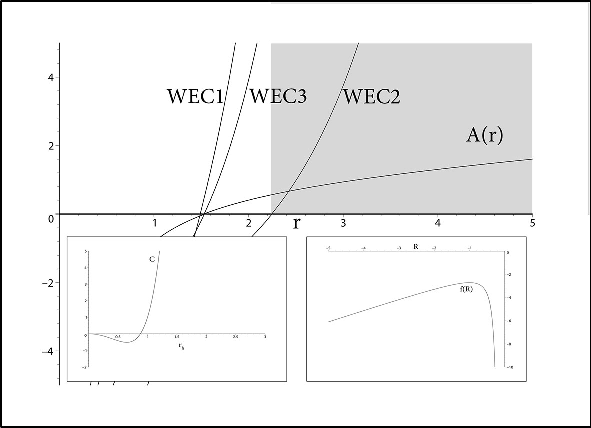
Figure 8: The model with $f\left(R\right)=R$e${}^{-\frac{1}{R}}$ gives a region in which WECs are satisfied. Furthermore, since $\frac{d^{2}f}{dR^{2}}=\frac{1}{R^{3}}e^{-\frac{1}{R}}<0$, it gives an unstable model. Beyond certain radius the specific heat is also positive which is required for thermodynamical stability.

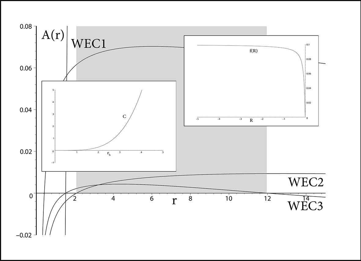
Figure 9: Our model in this case is given by $f\left(R\right)=R\left(e^{\frac{b}{R}}-1\right)$ with $b=const$. With the choice $b=1.1$ its observed that WECs are satisfied while the stability condition is violated in spite of the fact that the specific heat $C$ is everywhere positive.

4) Another interesting model of $f(R)$ gravity is given by 19

$$f\left(R\right)=R-\mu b\left[1-\left(1+\frac{R^{2}}{b^{2}}\right)^{-n}\right]$$ (31)

in which $\mu,b$ and $n$ are constants. Figure 4 with $\mu=1,b=1,n=-3$ shows that between horizon and a maximum radius we may have physical region in which $f^{\prime\prime}>0$. Now let’s consider 20 the model

$$f\left(R\right)=R-\mu b\frac{\left(\frac{R}{b}\right)^{2n}}{\left(\frac{R}{b}\right)^{2n}+1}$$ (32)

which amounts to the Fig. 5 and clearly there is no physical region.

5) Here, we use another model introduced in 21 which is given by

$$f\left(R\right)=R\left(1-c\right)+c\varepsilon\ln\left(\frac{\cosh\left(\frac{R}{\varepsilon}-b\right)}{\cosh\left(b\right)}\right)+\frac{R^{2}}{6m^{2}}$$ (33)

in which $c,\varepsilon,b$ and $\mu$ are all constants. Our analysis yields to the Fig. 6 with $c=\frac{1}{3}$ and Fig. 7 with $c=1.1$. One observes that although in Fig. 6 there is no physical region possible for different $c$ in Fig. 7 and for $r>r_{h}$ our physical conditions are satisfied provided $\left|R\right|<\left|R_{0}\right|$ where $R_{0}$ is the point for which $F\left(R\right)=0.$

6) In Ref. 22 an exponential form of $f(R)$ is introduced which is given by

$$f\left(R\right)=Re^{\frac{b}{R}}$$ (34)

in which $b=$constant with its first derivative

$$F\left(R\right)=e^{\frac{b}{R}}\left(1-\frac{b}{R}\right).$$ (35)

Our numerical plotting admits the Fig. 8 for this model with $b=-1$. We comment here that although the case $b=-1$ provides the WECs satisfied but in both cases $f^{\prime\prime}\left(R\right)$ is negative which makes the model not physical.

7) Another exponential model which is also given in 22 reads

$$f(R)=Re^{bR},$$ (36)

in which $b=$constant and

$$F(R)=e^{bR}\left(1+bR\right).$$ (37)

This does not satisfy the energy conditions and therefore it is not a physically interesting case.

8) In Ref. 23 a modified version of our models 6 and 7 is given in which

$$f(R)=R\left(e^{\frac{b}{R}}-1\right)$$

with $b=$constant and

$$F(R)=e^{\frac{b}{R}}\left(1-\frac{b}{R}\right)-1.$$

Figure 9 is our numerical results with $b=0.1$. For a bounded region from above and from below the WECs are satisfied while $f^{\prime\prime}\left(R\right)$ is negative which makes our model non-physical.

9) Among the exponential models of gravity let’s consider 24

$$f\left(R\right)=R+be^{\alpha R}$$ (38)

where $\alpha$ and $b$ are constants and

$$F\left(R\right)=1+b\alpha\text{ }e^{\alpha R}.$$

Figure 17 displays our numerical calculations for specific values of $\alpha=-1$ . Evidently from these figures we can conclude that this model is not a feasible model.

10) Finally we consider a model of gravity given in Ref. 25

$$f\left(R\right)=\left(\left|R\right|^{b}-\Lambda\right)^{\frac{1}{b}}$$ (39)

in which $b$ is a constant. The first derivative of the model is given by

$$F(R)=\left|R\right|^{b-1}\left(\left|R\right|^{b}-\Lambda\right)^{\frac{1}{b}-1}.$$

Figures 11 and 12 are with $b=\frac{1}{2}$ and $b=2,$ respectively, for $\Lambda=1.$ We observe that WECs are satisfied in a restricted region while for $b=2$ / $\frac{1}{2}$ it gives a stable / unstable model.

IV CONCLUSION

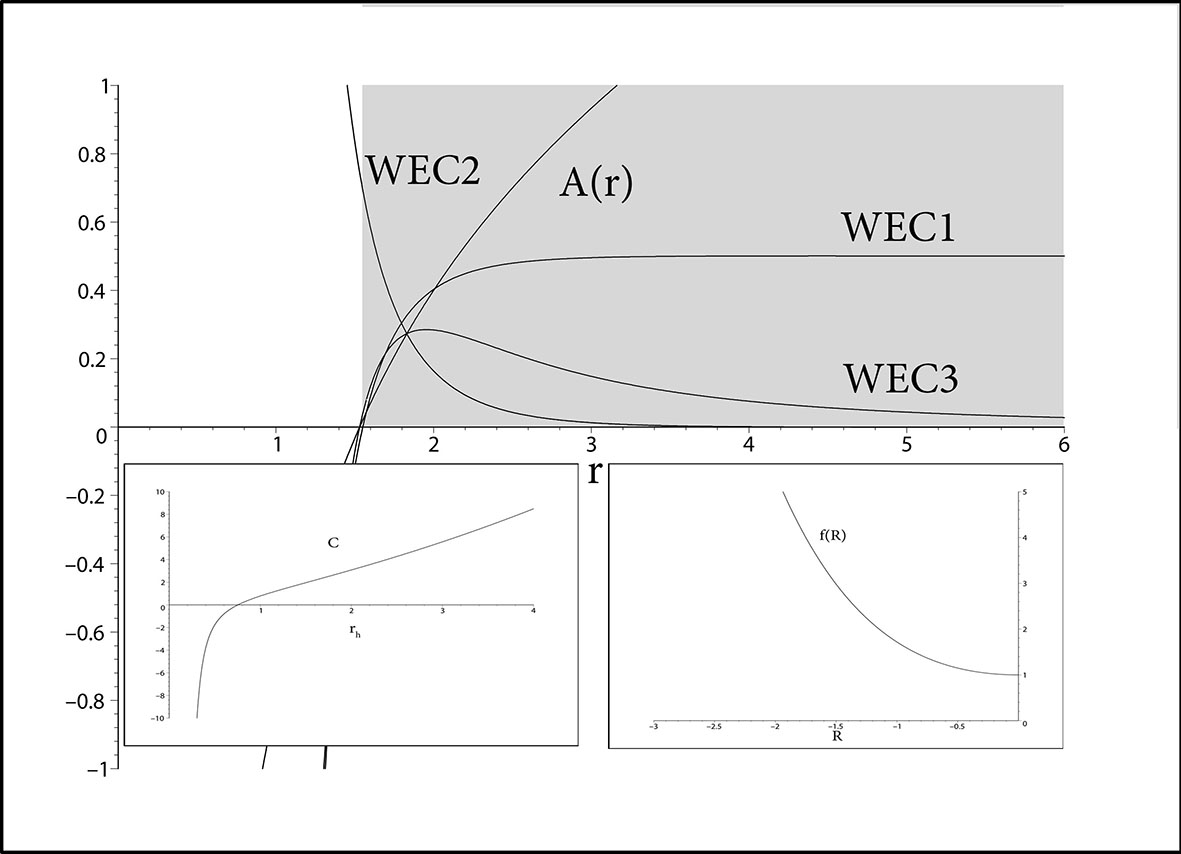
Figure 10: In this model we use $f\left(R\right)=R+be^{\alpha R}$ where $\alpha$ and $b$ are constants. For $\alpha=-1$ and $b=1,$ WECs are satisfied and $\frac{d^{2}f}{dR^{2}}>0$. Specific heat is shown also to be positive.

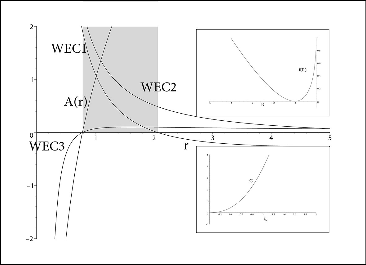
Figure 11: Our model is given by $f\left(R\right)=\left(\mid R\mid^{2}-1\right)^{2}$ which has WECs satisfied but $\frac{d^{2}f}{dR^{2}}>0$, for $\left|R\right|>\left|R_{0}\right|$ where $f^{\prime}\left(R_{0}\right)=0.$ This indicates stability of the solution. Furthermore the specific heat suggests a thermodynamically stable model too.

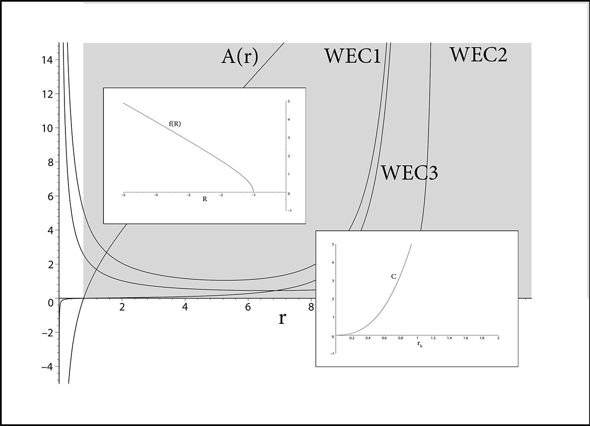
Figure 12: This is the model with $f\left(R\right)=\left(\mid R\mid^{\frac{1}{2}}-1\right)^{\frac{1}{2}}$ which has WECs conditions all satisfied while the stability condition is violated. It is thermodynamically stable since $C>0.$

In Einstein’s general relativity which corresponds to $f\left(R\right)=R$ , Rindler modification of the Schwarzschild metric faces the problem that the energy conditions are violated. For a resolution to this problem we invoke the large class of $f\left(R\right)$ theories. From cosmological standpoint the main reason that we insist on the Rindler acceleration term can be justified as follows: at large distances such a term may explain the flat rotation curves as well as the dark matter problem. Our physical source beside the gravitational curvature is taken to be a fluid with equal angular components. Being negative the radial pressure is repulsive in accordance with expectations of the dark energy. Our scan covered ten different $f\left(R\right)$ models and in most cases by tuning of the free parameters we show that WECs are satisfied. All over in ten different models we searched primarily for the validity of WECs as well as for $\frac{d^{2}f}{dR^{2}}>0$, i.e. the stability. With some effort thermodynamic stability can also be checked through the specific heat. With equal ease $\frac{df}{dR}>0,$ i.e. absence of ghost can be traced. Fig. 1 for instance, depicts the model with $f(R)=\sqrt{R^{2}+b^{2}}$, ($b=$constant) in which WECs and stability, even the thermodynamic stability are all satisfied, however, it hosts ghosts since $\frac{df}{dR}<0$ for $R<0$. Finally, among all models considered herein, we note that, Fig. 7 satisfies WECs, stability conditions as well as ghost free condition for $r>r_{\min}$ in which $r_{\min}\geq r_{h}$ depends on the other parameters.

Finally we comment that abundance of parameters in the $f\left(R\right)$ theories is one of its weak aspects. This weakness, however, may be used to obtain various limits and for this reason particular tuning of parameters is crucial. Our requirements have been weak energy conditions (WECs), Rindler acceleration, stability and absence of ghosts. Naturally further restrictions will add further constraints to dismiss some cases considered as viable in this study.

References

- (1) D. Grumiller, Phys. Rev. Lett. 105, 211303 (2010), 039901(E) (2011).
- (2) S. Carloni, D. Grumiller and F. Preis, Phys. Rev. D 83, 124024 (2011).
- (3) W. Rindler, ”Essential Relativity: Special, General, and Cosmological” revised second edition Springer-Verlay (1977).
- (4) L. Iorio, Mon. Not. R. Astron. Soc. 419, 2226 (2012);
- (5) L. Iorio, JCAP 05, 019 (2011); S. Carloni, D. Grumiller and F. Preis, Phys. Rev. D 83, 124024 (2011).
- (6) J. Sultana and D. Kazanas, Phys. Rev. D 85, 081502 (2012).
- (7) M. Milgrom, Astrophys. J. 270, 365 (1983).
- (8) M. Halilsoy, O. Gurtug and S. H. Mazharimousavi, arXiv:1212.2159.
- (9) S. H. Mazharimousavi and M. Halilsoy, Mod. Phys. Lett. A, 28, 1350073 (2013).
- (10) S. Nojiri and S. D. Odintsov, Phys. Rep. 505, 59 (2011).
- (11) A. De Felice, S. Tsujikawa, Living Rev. Rel. 13, 3 (2010).
- (12) T. P. Sotiriou and V. Faraoni, Rev. Mod. Phys. 82, 451 (2010).
- (13) S. Capozziello, V. F. Cardone, S. Carloni and A. Troisi, Phys. Latt. A 326, 292 (2004); C. Frigerio Martins and P. Salucci, Mon. Not. R. Astron. Soc. 381, 1103 (2007).
- (14) J. Santos, J. S. Alcaniz, M. J. Rebouças and F. C. Carvalho, Phys. Rev. D 76, 083513 (2007).
- (15) P. Mannheim, Prog. Part. Nucl. Phys. 56, 340 (2006); H. Culetu, Int. J. Mod. Phys. Conf. Ser. 3, 455 (2011); H. Culetu, Phys. Lett. A 376, 2817 (2012).
- (16) M. S. Movahed, S. Baghram and S. Rahvar, Phys. Rev. D 76, 044008 (2007).
- (17) S. Nojiri and S. Odintsov, Phys. Rev. D 68, 123512 (2003).
- (18) D. N. Vollick, Phys. Rev. D 69, 064030 (2004); I. Quiros and L. A. Ureña-López, Phys. Rev. D 82, 044002 (2010).
- (19) A. A. Starobinsky, J. Exp. Theor. Phys. Lett. 86, 157 (2007).
- (20) W. Hu and I. Sawicki, Phys. Rev. D, 76, 064004 (2007).
- (21) S. A. Appleby, R. A. Battye and A. A. Starobinsky JCAP 06, 005 (2010); S. A Appleby and R. A Battye, JCAP 05, 019 (2008).
- (22) L. Amendola, R. Gannouji, D. Polarski and S. Tsujikawa, Phys. Rev. D 75, 083504 (2007).
- (23) Z. Girones, A. Marchetti, O. Mena, C. Pena-Garay and N. Rius, JCAP 11, 004 (2010).
- (24) G. Cognola, E. Elizalde, S. Nojiri, S.D. Odintsov, L. Sebastiani, S. Zerbini, Phys.Rev. D77 (2008) 046009; E. Elizalde, S. Nojiri, S.D.Odintsov, L.Sebastiani, S. Zerbini. Phys.Rev. D 83, 086006 (2011).
- (25) L. Amendola and S. Tsujikawa, Phys. Lett. B 660, 125 (2008).