On the moment system and a flexible Prandtl number

Abstract

The Maxwell-Boltzmann moment system can be seen as a particular case of a mathematically more general moment system proposed by Machado in Ref. Machado (2013). This last moment system, whose integral generating form and a suggested continuous distribution are presented here, is used in this work to theoretically show (one of) its usefulness: A flexible Prandtl number can be obtained in both the Boltzmann equation and in the lattice Boltzmann equation with a conventional single relaxation time Bhatnagar-Gross-Krook collision model.

I Introduction

The Boltzmann equation (BE) (1) is used to describe the behavior of rarefied gases

$$\partial_{t}f+c_{\alpha}\partial_{\alpha}f=\frac{1}{\tau^{*}}(f^{\textrm{eq}}-f),$$ (1)

where the rhs is the nonlinear Bhatnagar-Gross-Krook (BGK) Bhatnagar et al. (1954) collision model. The main effect of the collision model is to bring the velocity distribution function closer to the local equilibrium state. $f$ represents the probability of finding a particle with velocity $\bm{c}$ at a certain position $\bm{x}$ and at certain time $t$. $f^{\textrm{eq}}\equiv f^{\textrm{eq}}(\rho,\bm{u},\theta,\bm{c})$ is the local equilibrium distribution function (EDF), with local flow velocity $\bm{u}$ and density $\rho$. $\theta=RT$, i.e. temperature in energy units, where $R$ is the specific gas constant and $T$ is the local temperature. Hence, the local equilibrium $f^{\textrm{eq}}$ is determined by the local conservative flow variables, i.e. density, the momentum and the energy. In the BE, $f^{\textrm{eq}}$ is usually the Maxwell-Boltzmann (MB) distribution function (more about this below). $\tau^{*}$ is the single relaxation time, which represents the relaxation process from the nonequilibrium state towards to a local equilibrium $f^{\textrm{eq}}$, and it is related to the viscosity of the fluid. However, based on an approach to obtain the macroscopic relations, e.g. method of moments on the Boltzmann equation (1) and using the MB moments, the result are macroscopic relations with the dimensionless Prandtl (Pr) number equal one. This, in contradiction to the physical Pr $=2/3$ for monatomic gases, which is important in the study of heat transport phenomena.

Several strategies are adopted to deal with that limitation, in order to get a correct Pr number. The ellipsoidal statistical (ES-BGK) approach is proposed in Holway Jr. (1963), Holway Jr. (1966), and the entropy condition (H-theorem) is later proven in Andries et al. (2000). The ES-BGK model contains a free parameter, which is useful to obtain the desired Pr number. This is achieved by only changing the stress tensor $\sigma$ via a flexible $b$ term. Another model is proposed by Shakhov in Shakhov (1968) (Shakhov-BGK), which only changes the heat flux $q$, and the H-theorem is proven near local equilibrium state Zheng and Struchtrup (2005). A construction, combining the aforementioned both models, is also found in the literature, c.f. Xu and Huang (2010), as a sum of both ES-BGK model and Shakhov-BGK model post-collision terms. This, in order to change both the stress tensor and heat flux simultaneously while maintaining a free parameter, useful to get the desired Pr number. Numerical comparisons between ES-BGK and Shakhov-BGK models are found in the literature, c.f. Mieussens and Struchtrup (2004), Meng et al. (2013a). In Liu (1990), a pure theoretical model is proposed by Liu, where both the stress tensor and the heat flux are changed by modifying the collision term in order to obtain an accepted Pr number.

However, unlike the present approach, those aforementioned constructions are: $i)$ designed, just having in mind, the macroscopic conservative relations, $ii)$ not necessarily as a result of the use of a general mathematical framework. Thus, the theoretical potential to go beyond the analyzed scales can be compromised. While the mean collision frequency in the ES-BGK, Shakhov-BGK and the Liu models are independent of the microscopic velocity, there are other models that use velocity dependent collision frequencies c.f. Bouchut and Perthame (1993), Struchtrup (1997), Zheng (2004), Mieussens and Struchtrup (2004).

Despite that some of the aforementioned construction have not been developed recently, there are many unanswered questions regarding their qualities, characteristics, performance, etc. Because of another view is presented in this work for the first time, some theoretical outcomes are outlined, and a complete treaty about it, cannot be claimed here either. Therefore, further theoretical work and numerical assessments for different flows (e.g. Poiseuille, Couette) deserve separate works and are presented by the author elsewhere.

The use of multiple relaxation time (MRT) is also another adopted strategy to obtain a realistic Pr number. For instance, in the lattice Boltzmann (LB) method (McNamara and Zanetti (1988), Higuera and Jimenez (1989), Higuera et al. (1989), Koelman (1991), Chen et al. (1992), Qian et al. (1992), Succi (2001),Hänel (2004), Guo and Shu (2013)), the MRT is very popular, c.f. d’Humiéres (1992), Lallemand and Luo (2003), Shan and Chen (2007), Philippi et al. (2007), Zheng et al. (2008), Chen et al. (2010), to mention few. For those unacquainted with the LB method, the continuous Boltzmann equation can be particularly discretized in both time and phase space He and Luo (1997), leading to the LBGK equation

$$f_{i}(\bm{x}+\bm{c}_{i}\delta t,t+\delta t)=f_{i}(\bm{x},t)+\frac{1}{\tau}(f_{i}^{\textrm{eq}}-f_{i}),$$ (2)

where $i=1,\dots,n_{q}$ and $n_{q}$ is the number of discrete lattice velocity vectors. In the LB method, the equilibrium $f^{\textrm{eq}}\equiv f^{\textrm{eq}}(\rho,\bm{u},\bm{c},\theta)$ is modeled, and also local. $\tau$ is the relaxation time, non-dimensionalized with $\delta t$. Within the LB method context, the terms $\bm{c}$, $\bm{u}$, $t$, $\bm{x}$ and $\theta$ are in lattice units (LU), c.f. Succi (2001). $f_{i}$ represents the probability of finding a particle with velocity $\bm{c}_{i}$ at position $\bm{x}$ and time $t$ in LU. Usually, the chosen denotation in the LB constructions follows the one in Qian et al. (1992), D$d$Q$(2z+1)^{d}$, but here the one-dimensional $z$ term (as defined in Machado (2013)) is used. $d$ is the dimension in this work. It should be pointed out that the use of more than one relaxation time has also a positive effect on the stability of the LB method, when compared to a single relaxation time LB method. Another strategy (in the LB method) is the use of the double distribution function approach He et al. (1998) (as the opposite to single distribution approach used in this work), which includes two relaxation times (TRT). The TRT strategy is also followed in Shan (1997). A modified BGK collision model is the chosen strategy in Gan et al. (2011).

Because of the LB method is a discretization of the Boltzmann equation then, it should not be a surprise that the aforecited strategies implemented within the Boltzmann equation context can also be used on the LB equation, c.f. Meng et al. (2013b). Another strategy, based on derivations involving the Fokker-Planck equation, is also found in Gorji et al. (2011), to obtain the correct Pr number of 2/3 for monatomic gases. However, the present work is focused on the BGK-BE (1) and LBGK equation (2), to theoretically show that they are enough to obtain a Pr number at will.

The rest of this work is organized as follows: Section II deals with the moment system. The derivation of the Prandtl number is carried out in section III and further discussions are found in section IV.

II On the moment system

One can argue that all those aforementioned approaches have been efforts to circumvent the shortcomings of the MB moments. In this work the adopted strategy is based on the results obtained by Machado in Machado (2013), where a new hydrodynamic moment system is proposed (c.f. table VI, Eqs. 50 and 51 therein). Although a new high-order LB construction is used to derivate the hydrodynamic moment system in Machado (2013), the results are not necessarily limited to such discrete constructions. Based on the work in Machado (2013), the moments can also be obtained from the following integral relation:

$$\int\Bigg{(}\underbrace{\frac{\rho}{(2\pi\theta\mathcal{F}_{n})^{d/2}}\textrm{\Large{{e}}}\Big{(}-\frac{(\bm{c}-\bm{u})^{2}}{2\theta\mathcal{F}_{n}}\Big{)}}_{I}\Bigg{)}\bm{c}^{n}d\bm{c}.\ \$$ (3)

The containing terms $\mathcal{F}_{n}^{m}$ (defined in Eq. (51) in Machado (2013)) are repeated in Eq. (4):

$$\mathcal{F}_{n}^{m_{\textrm{Max}}}=\prod_{m=0}^{m_{\textrm{Max}}-1}\frac{n-2m-\textrm{mod}(n-2m+1,2)+2\mu}{n-2m-\textrm{mod}(n-2m+1,2)}.\$$ (4)

The direct insertion of $\mathcal{F}_{n}^{m}$ for $m=1$, $\mu=0$, and $\mu\neq 0$ with $n=2,3$ into the $I$-term in Eq. (3) gives a continuous EDF with existing variance equal to $\theta\mathcal{F}_{n}$. Examples are depicted in Fig. 1. This suggests that instead of a MB distribution (i.e. $\mathcal{F}_{n}=1$ when $\mu=0$), the obtained EDF can be used to define a continuous EDF in the BE. The integral (3) can be evaluated thereafter to get the first fourth moments (counting from zero). In order to generate moments beyond the third-order, other special functions are needed in the $I$-term (c.f. Machado (2013)), whose theoretical analysis is out of the scope of this work. Nevertheless, the evaluation of Eq. (3) and the subsequent substitution of the terms $\mathcal{F}_{n}^{m}$ can be used as a practical integral-based generating procedure. This, in order to match the new moments, and to obtain the equations concerning the conservation laws. The first five convective moments can be written in the following form:

$$\int f^{\textrm{eq}}(\rho,\bm{u},\bm{c},\theta)d\bm{c} = \rho,$$ (5a)

$$j_{\alpha}=\int f^{\textrm{eq}}(\rho,\bm{u},\bm{c},\theta)c_{\alpha}d\bm{c} = \rho u_{\alpha},$$ (5b)

$$P_{\alpha,\beta}=\int f^{\textrm{eq}}(\rho,\bm{u},\bm{c},\theta)c_{\alpha}c_{\beta}d\bm{c} = \rho\Big{(}(2\mu+1)\delta_{\alpha,\beta}\theta+u_{\alpha}u_{\beta}\Big{)},$$ (5c)

$$Q_{\alpha,\beta,\Omega}=\int f^{\textrm{eq}}(\rho,\bm{u},\bm{c},\theta)c_{\alpha}c_{\beta}c_{\Omega}d\bm{c} = \rho\Bigg{[}\Bigg{(}\Big{(}\frac{2\mu}{1+\delta_{\alpha,\Omega}+\delta_{\alpha,\beta}}+1\Big{)}u_{\alpha}\delta_{\beta,\Omega}$$

$$+ \Big{(}\frac{2\mu}{\delta_{\beta,\Omega}+1+\delta_{\alpha,\beta}}+1\Big{)}u_{\beta}\delta_{\alpha,\Omega}$$

$$+ \Big{(}\frac{2\mu}{\delta_{\beta,\Omega}+\delta_{\alpha,\Omega}+1}+1\Big{)}u_{\Omega}\delta_{\alpha,\beta}\Bigg{)}\theta+u_{\alpha}u_{\beta}u_{\beta}\Bigg{]},$$

$$R_{\alpha,\beta,\Omega,\Omega}=\int f^{\textrm{eq}}(\rho,\bm{u},\bm{c},\theta)c_{\alpha}c_{\beta}c_{\Omega}^{2}d\bm{c} = \rho\Big{[}(2\mu+1)(2\mu+\delta_{\alpha,\beta}+\delta_{\alpha,\Omega}+\delta_{\Omega,\beta})\theta^{2}\delta_{\alpha,\beta}$$

$$+ (2\mu+\delta_{\alpha,\beta}+\delta_{\alpha,\Omega}+\delta_{\beta,\Omega})\theta u_{\alpha}u_{\beta}\delta_{\alpha,\beta}$$

$$+ (2\mu+2\delta_{\beta,\Omega}+1)\theta(u_{\alpha}\delta_{\beta,\Omega}+u_{\Omega}(\delta_{\alpha,\beta}-\delta_{\alpha,\Omega}))u_{\Omega}$$

$$+ u_{\alpha}\big{(}(2\mu+1)\theta(1-\delta_{\alpha,\beta})(1-\delta_{\beta,\Omega})$$

$$+ u_{\beta}^{2}\delta_{\beta,\Omega}+u_{\Omega}^{2}(1-\delta_{\beta,\Omega})\big{)}u_{\beta}\Big{]}.$$

$\delta_{\alpha,\beta}$ is the Kronecker delta, which equals to one when $\alpha=\beta$, otherwise is zero. $u_{\alpha}$ is the flow velocity on $\alpha$. The terms $\alpha$, $\beta$ and $\Omega$ are the three axes coordinate. The above integral representations are over the velocity space and are written in condense notation, so that for instance, in a two-dimensional case $Q_{\alpha,\beta,\beta}=\int f^{\textrm{eq}}(\bm{x},\bm{c},t)\bm{c}^{3}d\bm{c}=\int f^{\textrm{eq}}(\bm{x},\bm{c},t)c_{\alpha}c_{\beta}^{2}d\bm{c}$ means

$$Q_{\alpha,\beta,\beta} = \rho\int_{-\infty}^{\infty}\frac{1}{(2\pi\theta\mathcal{F}_{1})^{1/2}}\textrm{\Large{{e}}}\Big{(}\frac{(c_{\alpha}-u_{\alpha})^{2}}{2\mathcal{F}_{1}\theta}\Big{)}c_{\alpha}dc_{\alpha}$$

$$\times \int_{-\infty}^{\infty}\frac{1}{(2\pi\theta\mathcal{F}_{2})^{1/2}}\textrm{\Large{{e}}}\Big{(}\frac{(c_{\beta}-u_{\beta})^{2}}{2\mathcal{F}_{2}}\Big{)}c_{\beta}^{2}dc_{\beta}.$$

When $\mu=0$, the last three moments (5) are reduced to, e.g.:

$$P_{\alpha,\alpha} = \rho(\theta+u_{\alpha}^{2}),\qquad\ \ P_{\alpha,\beta}=\rho u_{\alpha}u_{\beta},$$

$$Q_{\alpha,\alpha,\alpha} = \rho(3\theta u_{\alpha}+u_{\alpha}^{3}),\ Q_{\alpha,\beta,\beta}=\rho(\theta u_{\alpha}+u_{\alpha}u_{\beta}^{2}),$$

$$Q_{\alpha,\beta,\Omega} = \rho(u_{\alpha}u_{\beta}u_{\Omega}),\ \ R_{\alpha,\alpha,\alpha,\alpha}=\rho(3\theta^{2}+6u_{\alpha}^{2}\theta+u_{\alpha}^{4}),$$

$$R_{\alpha,\beta,\beta,\beta} = \rho(3u_{\beta}\theta+u_{\beta}^{3})u_{\alpha},\ R_{\alpha,\beta,\Omega,\Omega}=\rho u_{\alpha}u_{\beta}(u_{\Omega}^{2}+\theta),$$

$$R_{\alpha,\alpha,\beta,\beta} = \rho(u_{\alpha}^{2}+\theta)(u_{\beta}^{2}+\theta),$$

which are (some of) their equivalent MB hydrodynamic moments. Recall that the above first five hydrodynamic convective moments, seen in Eqs. (5), represent the density ($\rho$), momentum density ($j$), pressure tensor ($P$), energy flux ($Q$), and the rate of change of the energy flux ($R$) respectively. Similarly, the central moments can be obtained, using the relations (5), e.g.:

$$\int f^{\textrm{eq}}d\bm{c}=\rho,$$ (8a)

$$\int f^{\textrm{eq}}(c_{\alpha}-u_{\alpha})d\bm{c}=0,$$ (8b)

$$\int f^{\textrm{eq}}(c_{\alpha}-u_{\alpha})(c_{\beta}-u_{\beta})d\bm{c}=\rho(2\mu+1)\delta_{\alpha,\beta}\theta,$$ (8c)

$$\int f^{\textrm{eq}}(c_{\alpha}-u_{\alpha})(c_{\beta}-u_{\beta})(c_{\Omega}-u_{\Omega})d\bm{c}$$ (8d)

$$=-4\rho\theta u_{\alpha}\mu\delta_{\alpha,\beta}\delta_{\beta,\Omega},$$

where Eq. (8d) is not always zero as in the MB moments. Note that in the new moment system (c.f. Eqs. (3), (5), (8) and (50)-(51) in Machado (2013)) all the hydrodynamic moments from the second-order and onward are modified when compared to the MB system. The shown rhs outputs in Eqs. (5) and (8) has been algebraically verified with the D$d$Q$(2z+1)^{d}$ lattice set using the high-order LB model proposed in Machado (2013) for $z$ up to 4 and $d=1,2,3$.

III On the Prandtl number

Based on an approach to obtain the macroscopic relations, e.g. method of moments on the Boltzmann equation (1) and using the relations (5) and (8), the mass continuity and the Navier-Stokes equations, (9a), (9), can be obtained (as in Machado (2013)). The resulting equation concerning the conservation of energy is included in this work. That is, a total of $d+2$ relations, where $d=3$:

$$\partial_{t}\rho+\partial_{\alpha}j_{\alpha} = 0,$$ (9a)

$$\rho\partial_{t}u_{\alpha}+\rho u_{\beta}\partial_{\beta}u_{\alpha} = -\partial_{\alpha}p+\partial_{\beta}\Bigg{[}\nu\Bigg{(}\partial_{\beta}u_{\alpha}$$

$$+ \partial_{\alpha}u_{\beta}-\Big{(}\frac{2}{3}\Big{)}(\partial_{\Omega}u_{\Omega})\delta_{\alpha,\beta}\Bigg{)}\Bigg{]},$$

$$\frac{3\rho}{2}\Big{(}\partial_{t}\theta^{*}+u_{\alpha}\partial_{\alpha}\theta^{*}\Big{)} = -\rho\theta^{*}\partial_{\alpha}u_{\alpha}-\partial_{\alpha}q_{\alpha}$$

$$- \sigma_{\alpha,\beta}\partial_{\beta}u_{\alpha}.\$$

$p=\rho(2\mu+1)\theta$ is the pressure, while $\nu=\rho(2\mu+1)\theta\tau^{*}$ is the kinematic viscosity, i.e. the $\theta$ value is re-scaled by $(2\mu+1)$. This outcome can also be valid for (2), where $\tau^{*}=(\tau-1/2)$, as seen in the literature, c.f. Eq. (7) in Machado (2012), Eq. (22) in Machado (2013). The re-scaling hints $\theta^{*}=\theta(2\mu+1)$ in (9) and with re-scaled heat flux $q_{\alpha}=-5/2\tau^{*}p(2\mu+1)\partial_{\alpha}\theta=-\kappa^{*}\partial_{\alpha}\theta$ and stress tensor $\sigma_{\alpha,\beta}=-2\tau^{*}p\partial_{\alpha}u_{\beta}=-2\mu^{*}\partial_{\alpha}u_{\beta}$, and later dividing Eq. (9) by $(2\mu+1)$ leads to the Pr number (dimensionless number of the ratio between $\mu^{*}$ and $\kappa^{*}$):

$$\textrm{Pr}=(2\mu+1)^{-1}.$$ (10)

For instance, for the case of Pr = 2/3, the $\mu=1/4$, which is an admissible variable in the proposed construction in Machado (2013). A comparison between one of the previous models, e.g. the popular ES-BGK model where the Pr=$(1-b)^{-1}$, and Eq. (10) shows where they coincide.

That is, both the stress tensor and heat flux are modified when the new system of moment (c.f. Eqs. (5)) is implemented.

IV Further discussions

Because of the novelty of the construction, obviously, there are still many open questions regarding the stability of the method in thermal mode. A theoretical study related to the H-theorem is not necessarily a trivial one. It deserves a separate work, which is presented by the author elsewhere. Even so, there is no guarantee of stability. For instance, despite the theoretical outcome in Andries et al. (2000), the ES-BGK-Burnett equations are unstable with the correct Pr number but stable when the plain BGK-Burnett equations are implemented Balakrishnan (1999), Agarwal et al. (2001), Agarwal and Yun (2002), Zheng and Struchtrup (2004). On the other hand, rather than a construction dealing with a limited number of modified moments as in Holway Jr. (1963), Shakhov (1968), Liu (1990), Xu and Huang (2010), a new system (i.e. Eqs. (3), (5), (8) and (50)-(51) in Machado (2013)) is adopted in this work.

If the LB construction in Machado (2013) is the chosen route for the numerical implementation, it should be pointed out that: $i$) There exist admissible $\mu$ values so that positive populations can be theoretically obtained over several ranges of valid $\theta$ (extreme) values. Admissible lattice flow velocities at those $\theta$ extreme values can also be found. They are presented elsewhere when needed, as these ranges depend on the implemented lattice set; $ii$) Although the choice of finite difference schemes is usually due to stability reasons, their implementations contradict the essence of the main LB idea (c.f. Succi (2001), Brownlee et al. (2008)); $iii$) As covered in the aforecited works on MRT, the use of more than one single relaxation time can enhance stability, which is always desirable. Because of the present construction gives already a flexible Prandtl number, the construction of a scheme with more than one relaxation time should focus mainly on stability. A work on this is also the subject of study by the author elsewhere.

In essence, this work reaffirms the theoretical superiority of the moment system proposed by Machado in Machado (2013), whose integral generating form is outlined here, over the MB moment system, at least when handling with the Eqs. (9) (in both isothermal mode in Machado (2013) and in thermal mode in this work). This is achieved by changing the targeted local equilibrium state, from the MB distribution function (c.f. $\mu=0$ in Fig. 1), to distributions originally proposed by Machado in Machado (2013) in discrete form, and suggested in this work in continuous form.

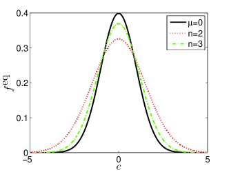
Figure 1: EDF ($f^{\textrm{eq}}$), i.e. $I$-term in Eq. (3), with $u=0$, $m=d=\rho=\theta=1$ and MB: $\mu=0$; Present: $\mu=1/4$, $n=2,3$.

Because of the proposed construction is a system, this opens for further works beyond the Navier-Stokes-Fourier equations, which are presented by the author elsewhere.

References

-
Machado (2013)
R. Machado,
On the generalized Hermite-based lattice Boltzmann
construction, lattice sets, weights, moments, distribution functions and
high-order models (2013), Submitted.
Pre-print on
URL: http://arxiv.org/abs/1304.4865. - Bhatnagar et al. (1954) P. L. Bhatnagar, E. P. Gross, and M. Krook, Phys. Rev. 94, 511 (1954).
- Holway Jr. (1963) L. H. Holway Jr., Ph.D. thesis, Harvard University, Department of Mathematics (1963).
- Holway Jr. (1966) L. H. Holway Jr., Phys. Fluids 9, 1658 (1966).
- Andries et al. (2000) P. Andries, P. L. Tallec, J.-P. Perlat, and B. Perthame, Eur. J. Mech. B-Fluid 19, 813 (2000).
- Shakhov (1968) E. M. Shakhov, Fluid Dynamics 9, 95 (1968).
- Zheng and Struchtrup (2005) Y. Zheng and H. Struchtrup, Phys. Fluids 17, 127103 (2005).
- Xu and Huang (2010) K. Xu and J.-C. Huang, J. Comp. Phys. Fluids 229, 7747 (2010).
- Mieussens and Struchtrup (2004) L. Mieussens and H. Struchtrup, Phys. Fluids 16, 2797 (2004).
- Meng et al. (2013a) J. Meng, L. Wu, J. Reese, and Y. Zhang, J. Comp. Phys. 251, 383 (2013a).
- Liu (1990) G. Liu, Phys. Fluids A 2, 227 (1990).
- Bouchut and Perthame (1993) F. Bouchut and B. Perthame, J. Stat. Phys. 71, 191 (1993).
- Struchtrup (1997) H. Struchtrup, Continuum Mech. Thermodyn. 9, 23 (1997).
- Zheng (2004) Y. Zheng, Ph.D. thesis, University of Victoria (2004).
- McNamara and Zanetti (1988) G. McNamara and G. Zanetti, Phys. Rev. Lett. 61, 2332 (1988).
- Higuera and Jimenez (1989) F. J. Higuera and J. Jimenez, Europhys. Lett. 9, 663 (1989).
- Higuera et al. (1989) F. J. Higuera, S. Succi, and R. Benzi, Europhys. Lett. 9, 345 (1989).
- Koelman (1991) J. M. V. A. Koelman, Europhys. Lett. 15, 603 (1991).
- Chen et al. (1992) H. Chen, S. Chen, and W. Matthaeus, Phys. Rev. A 45, R5339 (1992).
- Qian et al. (1992) Y. Qian, D. d’Humiéres, and P. Lallemand, Europhys. Lett. 17, 479 (1992).
- Succi (2001) S. Succi, The Lattice Boltzmann Equation: For Fluid Dynamics and Beyond (Oxford University Press, Oxford, 2001).
- Hänel (2004) D. Hänel, Molekulare Gasdynamik: Einführung in die kinetische Theorie der Gase und Lattice-Boltzmann-Methoden (Springer, Berling, 2004).
- Guo and Shu (2013) Z. Guo and C. Shu, Lattice Boltzmann Method and its Applications in Engineering (World Scientific, Singapore, 2013).
- d’Humiéres (1992) D. d’Humiéres, Prog. Astronaut. Aeronaut. 159, 450 (1992).
- Lallemand and Luo (2003) P. Lallemand and L.-S. Luo, Phys. Rev. E 68, 036706 (2003).
- Shan and Chen (2007) X. Shan and H. Chen, Internat. J. Modern Phys. C 18, 637 (2007).
- Philippi et al. (2007) P. C. Philippi, J. L. A. Hegele, R. Surmas, D. N. Siebert, and L. O. E. dos Santos, Int. J. Mod Phys C 18, 556 (2007).
- Zheng et al. (2008) L. Zheng, B. Shi, and Z. Guo, Phys. Rev. E 78, 026705 (2008).
- Chen et al. (2010) F. Chen, A. Xu, G. Zhang, Y. Li, and S. Succi, Europhys. Lett. 90, 54003 (2010).
- He and Luo (1997) X. He and L.-S. Luo, Phys. Rev. E 55, R6333 (1997).
- He et al. (1998) X. He, S. Chen, and G. D. Doolen, J. Comput. Phys. 146, 282 (1998).
- Shan (1997) X. Shan, Phys. Rev. E 55, 2780 (1997).
- Gan et al. (2011) Y. Gan, A.-G. Xu, G. Zhang, and Y. Li, Commun. Theor. Phys. 56, 490 (2011).
- Meng et al. (2013b) J. Meng, Y. Zhang, N. G. Hadjiconstantinou, G. A. Radtke, and X. Shan, J. Fluid Mech. 718, 347 (2013b).
- Gorji et al. (2011) M. H. Gorji, M. Torrilhon, and P. Jenny, J. Fluid Mech. 680, 574 (2011).
- Machado (2012) R. Machado, Math. Comp. Sim. 84, 26 (2012).
- Balakrishnan (1999) R. Balakrishnan, Ph.D. thesis, Whichita State University (1999).
- Agarwal et al. (2001) R. K. Agarwal, K.-Y. Yun, and R. Balakrishnan, Phys. Fluids 13, 3061 (2001).
- Agarwal and Yun (2002) R. K. Agarwal and K.-Y. Yun, Appl. Mech. Rev. 55, 219 (2002).
- Zheng and Struchtrup (2004) Y. Zheng and H. Struchtrup, Cont. Mech. Thermodyn 16, 97 (2004).
- Brownlee et al. (2008) R. Brownlee, A. Gorban, and J. Levesley, Phys. A 387, 385 (2008).