Measurement in the de Broglie-Bohm interpretation:
Double-slit, Stern-Gerlach and EPR-B

Abstract

We propose a pedagogical presentation of measurement in the de Broglie-Bohm interpretation. In this heterodox interpretation, the position of a quantum particle exists and is piloted by the phase of the wave function. We show how this position explains determinism and realism in the three most important experiments of quantum measurement: double-slit, Stern-Gerlach and EPR-B.

First, we demonstrate the conditions in which the de Broglie-Bohm interpretation can be assumed to be valid through continuity with classical mechanics.

Second, we present a numerical simulation of the double-slit experiment performed by Jönsson in 1961 with electrons. It demonstrates the continuity between classical mechanics and quantum mechanics: evolution of the probability density at various distances and convergence of the quantum trajectories to the classical trajectories when h tends to 0.

Third, we present an analytic expression of the wave function in the Stern-Gerlach experiment. This explicit solution requires the calculation of a Pauli spinor with a spatial extension. This solution enables to demonstrate the decoherence of the wave function and the three postulates of quantum measurement: quantization, the Born interpretation and wave function reduction. The spinor spatial extension also enables the introduction of the de Broglie-Bohm trajectories, which gives a very simple explanation of the particles’ impact and of the measurement process.

Finally, we study the EPR-B experiment, the Bohm version of the Einstein-Podolsky-Rosen experiment. Its theoretical resolution in space and time shows that a causal interpretation exists where each atom has a position and a spin. This interpretation avoids the flaw of the previous causal interpretation. We recall that a physical explanation of non-local influences is possible.

I Introduction

"I saw the impossible done".Bell_1982 This is how John Bell describes his inexpressible surprise in 1952 upon the publication of an article by David Bohm Bohm_1952 . The impossibility came from a theorem by John von Neumann outlined in 1932 in his book The Mathematical Foundations of Quantum Mechanics,vonNeumann which seemed to show the impossibility of adding "hidden variables" to quantum mechanics. This impossibility, with its physical interpretation, became almost a postulate of quantum mechanics, based on von Neumann’s indisputable authority as a mathematician. As Bernard d’Espagnat notes in 1979:

"At the university, Bell had, like all of us, received from his teachers a message which, later still, Feynman would brilliantly state as follows: "No one can explain more than we have explained here […]. We don’t have the slightest idea of a more fundamental mechanism from which the former results (the interference fringes) could follow". If indeed we are to believe Feynman (and Banesh Hoffman, and many others, who expressed the same idea in many books, both popular and scholarly), Bohm’s theory cannot exist. Yet it does exist, and is even older than Bohm’s papers themselves. In fact, the basic idea behind it was formulated in 1927 by Louis de Broglie in a model he called "pilot wave theory". Since this theory provides explanations of what, in "high circles", is declared inexplicable, it is worth consideration, even by physicists […] who do not think it gives us the final answer to the question "how reality really is."dEspagnat

And in 1987, Bell wonders about his teachers’ silence concerning the Broglie-Bohm pilot-wave:

"But why then had Born not told me of this ’pilot wave’? If only to point out what was wrong with it? Why did von Neumann not consider it? More extraordinarily, why did people go on producing "impossibility" proofs after 1952, and as recently as 1978? While even Pauli, Rosenfeld, and Heisenberg could produce no more devastating criticism of Bohm’s version than to brand it as "metaphysical" and "ideological"? Why is the pilot-wave picture ignored in text books? Should it not be taught, not as the only way, but as an antidote to the prevailing complacency? To show that vagueness, subjectivity and indeterminism are not forced on us by experimental facts, but through a deliberate theoretical choice?"Bell_1987

More than thirty years after John Bell’s questions, the interpretation of the de Broglie-Bohm pilot wave is still ignored by both the international community and the textbooks.

What is this pilot wave theory? For de Broglie, a quantum particle is not only defined by its wave function. He assumes that the quantum particle also has a position which is piloted by the wave function.Broglie_1927 However only the probability density of this position is known. The position exists in itself (ontologically) but is unknown to the observer. It only becomes known during the measurement.

The goal of the present paper is to present the Broglie-Bohm pilot-wave through the study of the three most important experiments of quantum measurement: the double-slit experiment which is the crucial experiment of the wave-particle duality, the Stern and Gerlach experiment with the measurement of the spin, and the EPR-B experiment with the problem of non-locality.

The paper is organized as follows. In section II, we demonstrate the conditions in which the de Broglie-Bohm interpretation can be assumed to be valid through continuity with classical mechanics. This involves the de Broglie-Bohm interpretation for a set of particles prepared in the same way. In section III, we present a numerical simulation of the double-slit experiment performed by Jönsson in 1961 with electrons Jonsson . The method of Feynman path integrals allows to calculate the time-dependent wave function. The evolution of the probability density just outside the slits leads one to consider the dualism of the wave-particle interpretation. And the de Broglie-Bohm trajectories provide an explanation for the impact positions of the particles. Finally, we show the continuity between classical and quantum trajectories with the convergence of these trajectories to classical trajectories when $h$ tends to $0$. In section IV, we present an analytic expression of the wave function in the Stern-Gerlach experiment. This explicit solution requires the calculation of a Pauli spinor with a spatial extension. This solution enables to demonstrate the decoherence of the wave function and the three postulates of quantum measurement: quantization, Born interpretation and wave function reduction. The spinor spatial extension also enables the introduction of the de Broglie-Bohm trajectories which gives a very simple explanation of the particles’ impact and of the measurement process. In section V, we study the EPR-B experiment, the Bohm version of the Einstein-Podolsky-Rosen experiment. Its theoretical resolution in space and time shows that a causal interpretation exists where each atom has a position and a spin. Finally, we recall that a physical explanation of non-local influences is possible.

II The de Broglie-Bohm interpretation

The de Broglie-Bohm interpretation is based on the following demonstration. Let us consider a wave function $\Psi(\textbf{x},t)$ solution to the Schrödinger equation:

$$i\hbar\frac{\partial\Psi(\mathbf{x},t)}{\partial t}=\mathcal{-}\frac{\hbar^{2}}{2m}\triangle\Psi(\mathbf{x},t)+V(\mathbf{x})\Psi(\mathbf{x},t)$$ (1)

$$\Psi(\mathbf{x},0)=\Psi_{0}(\mathbf{x}).$$ (2)

With the variable change $\Psi(\mathbf{x},t)=\sqrt{\rho^{\hbar}(\mathbf{x},t)}\exp(i\frac{S^{\hbar}(\textbf{x},t)}{\hbar})$, the Schrödinger equation can be decomposed into Madelung equations Madelung_1926 (1926):

$$\frac{\partial S^{\hbar}(\mathbf{x},t)}{\partial t}+\frac{1}{2m}(\nabla S^{\hbar}(\mathbf{x},t))^{2}+V(\mathbf{x})-\frac{\hbar^{2}}{2m}\frac{\triangle\sqrt{\rho^{\hbar}(\mathbf{x},t)}}{\sqrt{\rho^{\hbar}(\mathbf{x},t)}}=0$$ (3)

$$\frac{\partial\rho^{\hbar}(\mathbf{x},t)}{\partial t}+div\left(\rho^{\hbar}(\mathbf{x},t)\frac{\nabla S^{\hbar}(\mathbf{x},t)}{m}\right)=0$$ (4)

with initial conditions:

$$\rho^{\hbar}(\mathbf{x},0)=\rho^{\hbar}_{0}(\mathbf{x})\qquad\text{and}\qquad S^{\hbar}(\mathbf{x},0)=S^{\hbar}_{0}(\mathbf{x}).$$ (5)

Madelung equations correspond to a set of non-interacting quantum particles all prepared in the same way (same $\rho^{\hbar}_{0}(\mathbf{x})$ and $S^{\hbar}_{0}(\mathbf{x})$).

A quantum particle is said to be statistically prepared if its initial probability density $\rho^{\hbar}_{0}(\mathbf{x})$ and its initial action $S^{\hbar}_{0}(\mathbf{x})$ converge, when $\hbar\to 0$, to non-singular functions $\rho_{0}(\mathbf{x})$ and $S_{0}(\mathbf{x})$. It is the case of an electronic or $C_{60}$ beam in the double slit experiment or an atomic beam in the Stern and Gerlach experiment. We will seen that it is also the case of a beam of entrangled particles in the EPR-B experiment. Then, we have the following theorem: Gondran2011 ; Gondran2012a

For statistically prepared quantum particles, the probability density $\rho^{\hbar}(\textbf{x},t)$ and the action $S^{\hbar}(\textbf{x},t)$, solutions to the Madelung equations (3)(4)(5), converge, when $\hbar\to 0$, to the classical density $\rho(\textbf{x},t)$ and the classical action $S(\textbf{x},t)$, solutions to the statistical Hamilton-Jacobi equations:

$$\frac{\partial S\left(\textbf{x},t\right)}{\partial t}+\frac{1}{2m}(\nabla S(\textbf{x},t))^{2}+V(\textbf{x},t)=0$$ (6)

$$S(\textbf{x},0)=S_{0}(\textbf{x})$$ (7)

$$\frac{\partial\mathcal{\rho}\left(\textbf{x},t\right)}{\partial t}+div\left(\rho\left(\textbf{x},t\right)\frac{\nabla S\left(\textbf{x},t\right)}{m}\right)=0$$ (8)

$$\rho(\mathbf{x},0)=\rho_{0}(\mathbf{x}).$$ (9)

We give some indications on the demonstration of this theorem when the wave function $\Psi(\textbf{x},t)$ is written as a function of the initial wave function $\Psi_{0}(\textbf{x})$ by the Feynman paths integral Feynman :

$$\Psi(\textbf{x},t)=\int F(t,\hbar)\exp\left(\frac{i}{\hbar}S_{cl}(\textbf{x},t;\textbf{x}_{0}\right)\Psi_{0}(\textbf{x}_{0})d\textbf{x}_{0}$$ (10)

where $F(t,\hbar)$ is an independent function of x and of $\textbf{x}_{0}$. For a statistically prepared quantum particle, the wave function is written $\Psi(\textbf{x},t)=F(t,\hbar)\int\sqrt{\rho^{\hbar}_{0}(\mathbf{x}_{0})}\exp(\frac{i}{\hbar}(S^{\hbar}_{0}(\textbf{x}_{0})+S_{cl}(\textbf{x},t;\textbf{x}_{0}))d\textbf{x}_{0}$. The theorem of the stationary phase shows that, if $\hbar$ tends towards 0, we have $\Psi(\textbf{x},t)\sim\exp(\frac{i}{\hbar}min_{\textbf{x}_{0}}(S_{0}(\textbf{x}_{0})+S_{cl}(\textbf{x},t;\textbf{x}_{0}))$, that is to say that the quantum action $S^{h}(\textbf{x},t)$ converges to the function

$$S(\textbf{x},t)=min_{\textbf{x}_{0}}(S_{0}(\textbf{x}_{0})+S_{cl}(\textbf{x},t;\textbf{x}_{0}))$$ (11)

which is the solution to the Hamilton-Jacobi equation (6) with the initial condition (7). Moreover, as the quantum density $\rho^{h}(\textbf{x},t)$ satisfies the continuity equation (4), we deduce, since $S^{h}(\textbf{x},t)$ tends towards $S(\textbf{x},t)$, that $\rho^{h}(x,t)$ converges to the classical density $\rho(\textbf{x},t)$, which satisfies the continuity equation (8). We obtain both announced convergences.

These statistical Hamilton-Jacobi equations (6,7,8,9) correspond to a set of classical particles prepared in the same way (same $\rho_{0}(\mathbf{x})$ and $S_{0}(\mathbf{x})$). These classical particles are trajectories obtained in Eulerian representation with the velocity field $\mathbf{v}\left(\mathbf{x,}t\right)=\frac{\mathbf{\nabla}S\left(\mathbf{x,}t\right)}{m}$, but the density and the action are not sufficient to describe it completely. To know its position at time $t$, it is necessary to know its initial position. Because the Madelung equations converge to the statistical Hamilton-Jacobi equations, it is logical to do the same in quantum mechanics. We conclude that a statistically prepared quantum particle is not completely described by its wave function. It is necessary to add this initial position and an equation to define the evolution of this position in the time. It is the de Brogglie-Bohm interpretation where the position is called the "hidden variable".

The two first postulates of quantum mechanics, describing the quantum state and its evolution, CT_1977 must be completed in this heterodox interpretation. At initial time t=0, the state of the particle is given by the initial wave function $\Psi_{0}(\textbf{x})$ (a wave packet) and its initial position $\textbf{X}(0)$; it is the new first postulate. The new second postulate gives the evolution on the wave function and on the position. For a single spin-less particle in a potential $V(\textbf{x})$, the evolution of the wave function is given by the usual Schrödinger equation (1,2) and the evolution of the particle position is given by

$$\frac{d\textbf{X}(t)}{dt}=\frac{\textbf{J}^{h}(\textbf{x},t)}{\rho^{h}(\textbf{x},t)}|_{\textbf{x}=\textbf{X}(t)}=\frac{\nabla S^{h}(\textbf{x},t)}{m}|_{\textbf{x}=\textbf{X}(t)}$$ (12)

where

$$\textbf{J}^{h}(\textbf{x},t)=\frac{\hbar}{2mi}(\Psi^{*}(\textbf{x},t)\nabla\Psi(\textbf{x},t)-\Psi(\textbf{x},t)\nabla\Psi^{*}(\textbf{x},t))$$ (13)

is the usual quantum current.

In the case of a particle with spin, as in the Stern and Gerlach experiment, the Schrödinger equation must be replaced by the Pauli or Dirac equations.

The third quantum mechanics postulate which describes the measurement operator (the observable) can be conserved. But the three postulates of measurement are not necessary: the postulate of quantization, the Born postulate of probabilistic interpretation of the wave function and the postulate of the reduction of the wave function. We see that these postulates of measurement can be explained on each example as we will shown in the following.

We replace these three postulates by a single one, the "quantum equilibrium hypothesis", Durr_1992 ; Sanz ; Norsen that describes the interaction between the initial wave function $\Psi_{0}(\textbf{x})$ and the initial particle position $\textbf{X}(0)$: For a set of identically prepared particles having $t=0$ wave function $\Psi_{0}(\textbf{x})$, it is assumed that the initial particle positions $\textbf{X}(0)$ are distributed according to:

$$P[\textbf{X}(0)=\textbf{x}]\equiv P(\textbf{x},0)=|\Psi_{0}(\textbf{x})|^{2}=\rho^{h}_{0}(\textbf{x}).$$ (14)

It is the Born rule at the initial time.

Then, the probability distribution ($P(\textbf{x},t)\equiv P[\textbf{X}(t)=\textbf{x}]$) for a set of particles moving with the velocity field $\textbf{v}^{h}(\textbf{x},t)=\frac{\nabla S^{h}(\textbf{x},t)}{m}$ satisfies the property of the "equivariance" of the $|\Psi(\textbf{x},t)|^{2}$ probability distribution: Durr_1992

$$P[\textbf{X}(t)=\textbf{x}]\equiv P(\textbf{x},t)=|\Psi(\textbf{x},t)|^{2}=\rho^{h}(\textbf{x},t).$$ (15)

It is the Born rule at time t.

Then, the de Broglie-Bohm interpretation is based on a continuity between classical and quantum mechanics where the quantum particles are statistical prepared with an initial probability densitiy satisfies the "quantum equilibrium hypothesis" (14). It is the case of the three studied experiments.

We will revisit these three measurement experiments through mathematical calculations and numerical simulations. For each one, we present the statistical interpretation that is common to the Copenhagen interpretation and the de Broglie-Bohm pilot wave, then the trajectories specific to the de Broglie-Bohm interpretation. We show that the precise definition of the initial conditions, i.e. the preparation of the particles, plays a fundamental methodological role.

III Double-slit experiment with electrons

Young’s double-slit experimentYoung_1802 has long been the crucial experiment for the interpretation of the wave-particle duality. There have been realized with massive objects, such as electrons Davisson ; Jonsson , neutrons Halbon , cold neutrons Zeilinger_1988 , atoms Estermann , and more recently, with coherent ensembles of ultra-cold atoms Shimizu , and even with mesoscopic single quantum objects such as C₆₀ and C₇₀ Arndt . For Feynman, this experiment addresses "the basic element of the mysterious behavior [of electrons] in its most strange form. [It is] a phenomenon which is impossible, absolutely impossible to explain in any classical way and which has in it the heart of quantum mechanics. In reality, it contains the only mystery." Feynman_1965 The de Broglie-Bohm interpretation and the numerical simulation help us here to revisit the double-slit experiment with electrons performed by Jönsson in 1961 and to provide an answer to Feynman’mystery. These simulations Gondran_2005a follow those conducted in 1979 by Philippidis, Dewdney and Hiley Philippidis_1979 which are today a classics. However, these simulations Philippidis_1979 have some limitations because they did not consider realistic slits. The slits, which can be clearly represented by a function $G(y)$ with $G(y)=1$ for $-\beta\leq y\leq\beta$ and $G(y)=0$ for $|y|>\beta$, if they are $2\beta$ in width, were modeled by a Gaussian function $G(y)=e^{-y^{2}/2\beta^{2}}$. Interference was found, but the calculation could not account for diffraction at the edge of the slits. Consequently, these simulations could not be used to defend the de Broglie-Bohm interpretation.

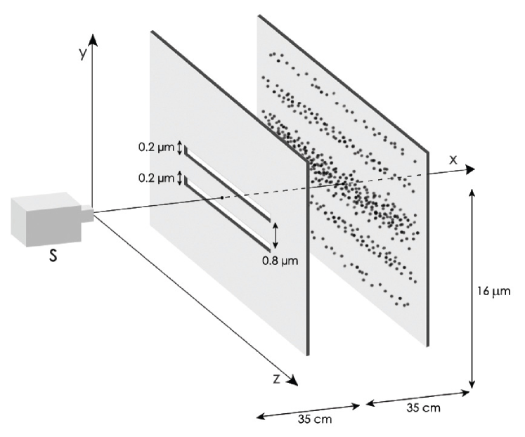
Figure 1: Diagram of the Jönnson’s double slit experiment performed with electrons.

Figure 1 shows a diagram of the double slit experiment by Jönsson. An electron gun emits electrons one by one in the horizontal plane, through a hole of a few micrometers, at a velocity $v=1.8\times 10^{8}m/s$ along the horizontal $x$-axis. After traveling for $d_{1}=35cm$, they encounter a plate pierced with two horizontal slits A and B, each $0.2\mu$m wide and spaced $1\mu$m from each other. A screen located at $d_{2}=35cm$ after the slits collects these electrons. The impact of each electron appears on the screen as the experiment unfolds. After thousands of impacts, we find that the distribution of electrons on the screen shows interference fringes.

The slits are very long along the $z$-axis, so there is no effect of diffraction along this axis. In the simulation, we therefore only consider the wave function along the $y$-axis; the variable $x$ will be treated classically with $x=vt$. Electrons emerging from an electron gun are represented by the same initial wave function $\Psi_{0}(y)$.

III.1 Probability density

Figure 2 gives a general view of the evolution of the probability density from the source to the detection screen (a lighter shade means that the density is higher i.e. the probability of presence is high). The calculations were made using the method of Feynman path integrals Gondran_2005a . The wave function after the slits ($t_{1}=d_{1}/v\simeq 2.10^{-11}s<t<t_{1}+d_{2}/v\simeq 4.10^{-11}s$) is deduced from the values of the wave function at slits A and B: $\Psi(y,t)=\Psi_{A}(y,t)+\Psi_{B}(y,t)$ with $\Psi_{A}(y,t)=\int_{A}K(y,t,y_{a},t_{1})\Psi(y_{a},t_{1})dy_{a}$, $\Psi_{B}(y,t)=\int_{B}K(y,t,y_{b},t_{1})\Psi(y_{b},t_{1})dy_{b}$ and $K(y,t,y_{\alpha},t_{1})=(m/2i\hbar(t-t_{1}))^{1/2}e^{im(y-y_{\alpha})^{2}/2\hbar(t-t_{1})}$.

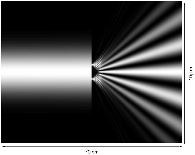
Figure 2: General view of the evolution of the probability density from the source to the screen in the Jönsson experiment. A lighter shade means that the density is higher i.e. the probability of presence is high.

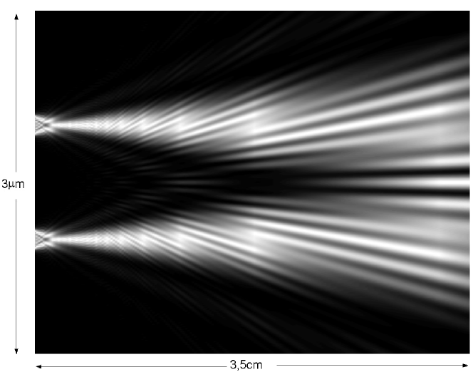
Figure 3: Close-up of the evolution of the probability density in the first $3cm$ after the slits in the Jönsson experiment.

Figure 3 shows a close-up of the evolution of the probability density just after the slits. We note that interference will only occur a few centimeters after the slits. Thus, if the detection screen is $1cm$ from the slits, there is no interference and one can determine by which slit each electron has passed. In this experiment, the measurement is performed by the detection screen, which only reveals the existence or absence of the fringes.

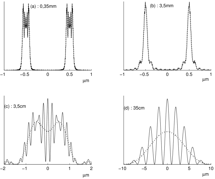
Figure 4: Comparison of the probability density $|\Psi_{A}+\Psi_{B}|^{2}$ (full line) and $|\Psi_{A}|^{2}+|\Psi_{B}|^{2}$ (dotted line) at various distances after the slits: (a) $0.35mm$, (b): $3.5mm$, (c): $3.5cm$ and (d): $35cm$.

The calculation method enables us to compare the evolution of the cross-section of the probability density at various distances after the slits ($0.35mm$, $3.5mm$, $3.5cm$ and $35cm$) where the two slits A and B are open simultaneously (interference: $|\Psi_{A}+\Psi_{B}|^{2}$) with the evolution of the sum of the probability densities where the slits A and B are open independently (the sum of two diffractions: $|\Psi_{A}|^{2}+|\Psi_{B}|^{2}$). Figure 4 shows that the difference between these two phenomena appears only a few centimeters after the slits.

III.2 Impacts on screen and de Broglie-Bohm trajectories

The interference fringes are observed after a certain period of time when the impacts of the electrons on the detection screen become sufficiently numerous. Classical quantum theory only explains the impact of individual particles statistically.

However, in the de Broglie-Bohm interpretation: a particle has an initial position and follows a path whose velocity at each instant is given by equation (12). On the basis of this assumption we conduct a simulation experiment by drawing random initial positions of the electrons in the initial wave packet ("quantum equilibrium hypothesis").

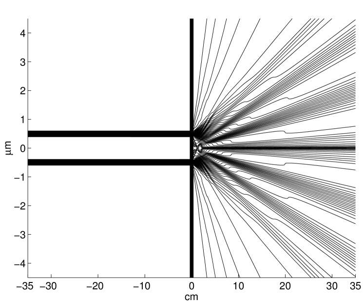
Figure 5: 100 electron trajectories for the Jönsson experiment.

Figure 5 shows, after its initial starting position, 100 possible quantum trajectories of an electron passing through one of the two slits: We have not represented the paths of the electron when it is stopped by the first screen. Figure 6 shows a close-up of these trajectories just after they leave their slits.

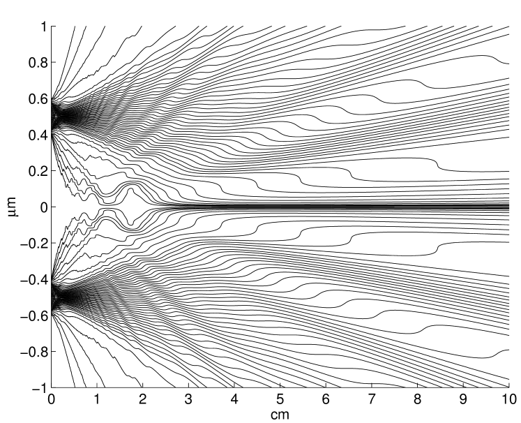
Figure 6: Close-up on the 100 trajectories of the electrons just after the slits.

The different trajectories explain both the impact of electrons on the detection screen and the interference fringes. This is the simplest and most natural interpretation to explain the impact positions: "The position of an impact is simply the position of the particle at the time of impact." This was the view defended by Einstein at the Solvay Congress of 1927. The position is the only measured variable of the experiment.

In the de Broglie-Bohm interpretation, the impacts on the screen are the real positions of the electron as in classical mechanics and the three postulates of the measurement of quantum mechanics can be trivialy explained: the position is an eigenvalue of the position operator because the position variable is identical to its operator (X$\Psi$ = x$\Psi$), the Born postulate is satisfied with the "equivariance" property, and the reduction of the wave packet is not necessary to explain the impacts.

Through numerical simulations, we will demonstrate how, when the Planck constant $h$ tends to 0, the quantum trajectories converge to the classical trajectories. In reality a constant is not able to tend to 0 by definition. The convergence to classical trajectories is obtained if the term $ht/m\rightarrow 0$; so $h\rightarrow 0$ is equivalent to $m\rightarrow+\infty$ (i.e. the mass of the particle grows) or $t\rightarrow 0$ (i.e. the distance slits-screem $d_{2}\rightarrow 0$). Figure 7 shows the 100 trajectories that start at the same 100 initial points when Planck’s constant is divided respectively by 10, 100, 1000 and 10000 (equivalent to multiplying the mass by 10, 100, 1000 and 10000). We obtain quantum trajectories converging to the classical trajectories, when $h$ tends to 0.

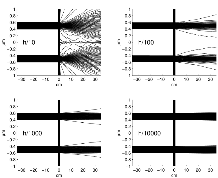
Figure 7: Convergence of 100 electron trajectories when h is divided by 10, 100, 1 000 and 10 000.

The study of the slits clearly shows that, in the de Broglie-Bohm interpretation, there is no physical separation between quantum mechanics and classical mechanics. All particles have quantum properties, but specifically quantum behavior only appears in certain experimental conditions: here when the ratio ht/m is sufficiently large. Interferences only appear gradually and the quantum particle behaves at any time as both a wave and a particle.

IV The Stern-Gerlach experiment

In 1922, by studying the deflection of a beam of silver atoms in a strongly inhomogeneous magnetic field (cf. Figure 8) Otto Stern and Walter Gerlach SternGerlach obtained an experimental result that contradicts the common sense prediction: the beam, instead of expanding, splits into two separate beams giving two spots of equal intensity $N^{+}$ and $N^{-}$ on a detector, at equal distances from the axis of the original beam.

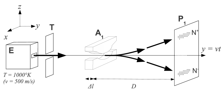
Figure 8: Schematic configuration of the Stern-Gerlach experiment.

Historically, this is the experiment which helped establish spin quantization. Theoretically, it is the seminal experiment posing the problem of measurement in quantum mechanics. Today it is the theory of decoherence with the diagonalization of the density matrix that is put forward to explain the first part of the measurement process Zeh . However, although these authors consider the Stern-Gerlach experiment as fundamental, they do not propose a calculation of the spin decoherence time.

We present an analytical solution to this decoherence time and the diagonalization of the density matrix. This solution requires the calculation of the Pauli spinor with a spatial extension as the equation:

$$\Psi^{0}(z)=(2\pi\sigma_{0}^{2})^{-\frac{1}{2}}e^{-\frac{z^{2}}{4\sigma_{0}^{2}}}\left(\begin{array}[]{c}\cos\frac{\theta_{0}}{2}e^{-i\frac{\varphi_{0}}{2}}\\ \sin\frac{\theta_{0}}{2}e^{i\frac{\varphi_{0}}{2}}\end{array}\right).$$ (16)

Quantum mechanics textbooks Feynman_1965 ; CT_1977 ; Sakurai ; LeBellac do not take into account the spatial extension of the spinor (16) and simply use the simplified spinor without spatial extension:

$$\Psi^{0}=\left(\begin{array}[]{c}\cos\frac{\theta_{0}}{2}e^{-i\frac{\varphi_{0}}{2}}\\ \sin\frac{\theta_{0}}{2}e^{i\frac{\varphi_{0}}{2}}\end{array}\right).$$ (17)

However, as we shall see, the different evolutions of the spatial extension between the two spinor components will have a key role in the explanation of the measurement process. This spatial extension enables us, in following the precursory works of Takabayasi Takabayasi_1954 , Bohm Bohm_1955 ; Bohm_1993 , Dewdney et al. Dewdney_1986 and Holland Holland_1993 , to revisit the Stern and Gerlach experiment, to explain the decoherence and to demonstrate the three postulates of the measure: quantization, Born statistical interpretation and wave function reduction.

Silver atoms contained in the oven E (Figure 8) are heated to a high temperature and escape through a narrow opening. A second aperture, T, selects those atoms whose velocity, $\textbf{v}_{0}$, is parallel to the $y$-axis. The atomic beam crosses the gap of the electromagnet $A_{1}$ before condensing on the detector, $P_{1}$ . Before crossing the electromagnet, the magnetic moment of each silver atom is oriented randomly (isotropically). In the beam, we represent each atom by its wave function; one can assume that at the entrance to the electromagnet, $A_{1}$, and at the initial time $t=0$, each atom can be approximatively described by a Gaussian spinor in $z$ given by (16) corresponding to a pure state. The variable $y$ will be treated classically with $y=vt$. $\sigma_{0}=10^{-4}m$ corresponds to the size of the slot T along the $z$-axis. The approximation by a Gaussian initial spinor will allow explicit calculations. Because the slot is much wider along the $x$-axis, the variable $x$ will be also treated classically. To obtain an explicit solution of the Stern-Gerlach experiment, we take the numerical values used in the CohenTannoudji textbook CT_1977 . For the silver atom, we have $m=1.8\times 10^{-25}kg$, $v_{0}=500\ m/s$ (corresponding to the temperature of $T=1000\textdegree K$). In equation (16) and in figure 9, $\theta_{0}$ and $\varphi_{0}$ are the polar angles characterizing the initial orientation of the magnetic moment, $\theta_{0}$ corresponds to the angle with the $z$-axis. The experiment is a statistical mixture of pure states where the $\theta_{0}$ and the $\varphi_{0}$ are randomly chosen: $\theta_{0}$ is drawn in a uniform way from $[0,\pi]$ and that $\varphi_{0}$ is drawn in a uniform way from $[0,2\pi]$.

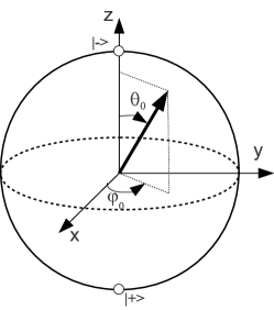
Figure 9: Orientation of the magnetic moment. $\theta_{0}$ and $\varphi_{0}$ are the polar angles characterizing the spin vector in the de Broglie-Bohm interpretation.

The evolution of the spinor $\Psi=\left(\begin{array}[]{c}\psi_{+}\\ \psi_{-}\end{array}\right)$ in a magnetic field B is then given by the Pauli equation:

$$i\hbar\left(\begin{array}[]{c}\frac{\partial\psi_{+}}{\partial t}\\ \frac{\partial\psi_{-}}{\partial t}\end{array}\right)=-\frac{\hbar^{2}}{2m}\Delta\left(\begin{array}[]{c}\psi_{+}\\ \psi_{-}\end{array}\right)+\mu_{B}\textbf{B}\sigma\left(\begin{array}[]{c}\psi_{+}\\ \psi_{-}\end{array}\right)$$ (18)

where $\mu_{B}=\frac{e\hbar}{2m_{e}}$ is the Bohr magneton and where $\sigma=(\sigma_{x},\sigma_{y},\sigma_{z})$ corresponds to the three Pauli matrices. The particle first enters an electromagnetic field B directed along the $z$-axis, $B_{x}=B^{\prime}_{0}x$, $B_{y}=0$, $B_{z}=B_{0}-B^{\prime}_{0}z$, with $B_{0}=5$ Tesla, $B^{\prime}_{0}=\left|\frac{\partial B}{\partial z}\right|=10^{3}~{}Tesla/m$ over a length $\Delta l=1~{}cm$. On exiting the magnetic field, the particle is free until it reaches the detector $P_{1}$ placed at a $D=20~{}cm$ distance.

The particle stays within the magnetic field for a time $\Delta t=\frac{\Delta l}{v}=2\times 10^{-5}s$. During this time $[0,\Delta t]$, the spinor is: Platt_1992 (see Appendix A)

$$\Psi(z,t)\simeq\left(\begin{array}[]{c}\cos\frac{\theta_{0}}{2}(2\pi\sigma_{0}^{2})^{-\frac{1}{2}}e^{-\frac{(z-\frac{\mu_{B}B^{\prime}_{0}}{2m}t^{2})^{2}}{4\sigma_{0}^{2}}}e^{i\frac{\mu_{B}B^{\prime}_{0}tz-\frac{\mu^{2}_{B}B^{\prime 2}_{0}}{6m}t^{3}+\mu_{B}B_{0}t+\frac{\hbar\varphi_{0}}{2}}{\hbar}}\\ i\sin\frac{\theta_{0}}{2}(2\pi\sigma_{0}^{2})^{-\frac{1}{2}}e^{-\frac{(z+\frac{\mu_{B}B^{\prime}_{0}}{2m}t^{2})^{2}}{4\sigma_{0}^{2}}}e^{i\frac{-\mu_{B}B^{\prime}_{0}tz-\frac{\mu^{2}_{B}B^{\prime 2}_{0}}{6m}t^{3}-\mu_{B}B_{0}t-\frac{\hbar\varphi_{0}}{2}}{\hbar}}\end{array}\right).$$ (19)

After the magnetic field, at time $t+\Delta t$ $(t\geq 0)$ in the free space, the spinor becomes: Bohm_1993 ; Dewdney_1986 ; Holland_1993 ; Platt_1992 ; Gondran_2005b (see Appendix A)

$$\Psi(z,t+\Delta t)\simeq\left(\begin{array}[]{c}\cos\frac{\theta_{0}}{2}(2\pi\sigma_{0}^{2})^{-\frac{1}{2}}e^{-\frac{(z-z_{\Delta}-ut)^{2}}{4\sigma_{0}^{2}}}e^{i\frac{muz+\hbar\varphi_{+}}{\hbar}}\\ \sin\frac{\theta_{0}}{2}(2\pi\sigma_{0}^{2})^{-\frac{1}{2}}e^{-\frac{(z+z_{\Delta}+ut)^{2}}{4\sigma_{0}^{2}}}e^{i\frac{-muz+\hbar\varphi_{-}}{\hbar}}\end{array}\right)$$ (20)

where

$$z_{\Delta}=\frac{\mu_{B}B^{\prime}_{0}(\Delta t)^{2}}{2m}=10^{-5}m,~{}~{}~{}~{}~{}~{}u=\frac{\mu_{B}B^{\prime}_{0}(\Delta t)}{m}=1m/s.$$ (21)

Equation (20) takes into account the spatial extension of the spinor and we note that the two spinor components have very different $z$ values. All interpretations are based on this equation.

IV.1 The decoherence time

We deduce from (20) the probability density of a pure state in the free space after the electromagnet:

$$\rho_{\theta_{0}}(z,t+\Delta t)\simeq(2\pi\sigma_{0}^{2})^{-\frac{1}{2}} \left(\cos^{2}\frac{\theta_{0}}{2}e^{-\frac{(z-z_{\Delta}-ut)^{2}}{2\sigma_{0}^{2}}}\right.$$ (22)

$$\quad+\left.\sin^{2}\frac{\theta_{0}}{2}e^{-\frac{(z+z_{\Delta}+ut)^{2}}{2\sigma_{0}^{2}}}\right)$$

Figure 10 shows the probability density of a pure state (with $\theta_{0}=\pi/3$) as a function of $z$ at several values of $t$ (the plots are labeled $y=vt$). The beam separation does not appear at the end of the magnetic field ($1~{}cm$), but $16~{}cm$ further along. It is the moment of the decoherence.

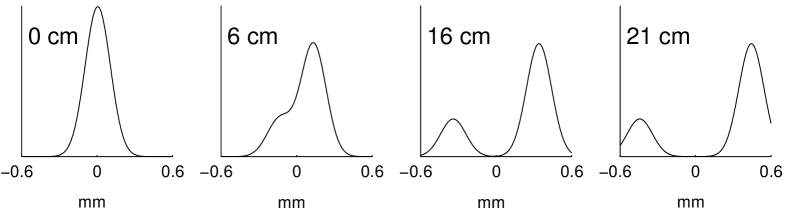
Figure 10: Evolution of the probability density of a pure state with $\theta_{0}=\pi/3$.

The decoherence time, where the two spots $N^{+}$ and $N^{-}$ are separated, is then given by the equation:

$$t_{D}\simeq\frac{3\sigma_{0}-z_{\Delta}}{u}=3\times 10^{-4}s.$$ (23)

This decoherence time is usually the time required to diagonalize the marginal density matrix of spin variables associated with a pure state Roston :

$$\rho^{S}(t)=\left(\begin{array}[]{ccccc}\int|\psi_{+}(z,t)|^{2}dz&\int\psi_{+}(z,t)\psi^{*}_{-}(z,t)dz\\ \int\psi_{-}(z,t)\psi^{*}_{+}(z,t)dz&\int|\psi_{-}(z,t)|^{2}dz\\ \end{array}\right)$$ (24)

For $t\geq t_{D}$, the product $\psi_{+}(z,t+\Delta t)\psi_{-}(z,t+\Delta t)$ is null and the density matrix is diagonal: the probability density of the initial pure state (20) is diagonal:

$$\rho^{S}(t+\Delta t)=(2\pi\sigma_{0}^{2})^{-1}\left(\begin{array}[]{ccccc}\cos^{2}\frac{\theta_{0}}{2}&0\\ 0&\sin^{2}\frac{\theta_{0}}{2}\\ \end{array}\right)$$ (25)

IV.2 Proof of the postulates of quantum measurement

We then obtain atoms with a spin oriented only along the $z$-axis (positively or negatively). Let us consider the spinor $\Psi(z,t+\Delta t)$ given by equation (20). Experimentally, we do not measure the spin directly, but the $\widetilde{z}$ position of the particle impact on $P_{1}$ (Figure 11).

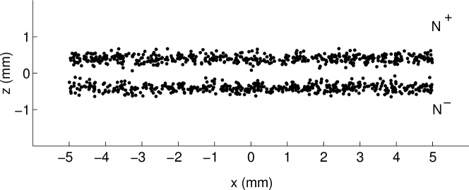
Figure 11: 1000 silver atom impacts on the detector $P_{1}$.

If  $\widetilde{z}\in N^{+}$, the term $\psi_{-}$ of (20) is numerically equal to zero and the spinor $\Psi$ is proportional to $\binom{1}{0}$, one of the eigenvectors of the spin operator $S_{z}=\frac{\hbar}{2}\sigma_{z}$: $\Psi(\tilde{z},t+\Delta t)\simeq(2\pi\sigma_{0}^{2})^{-\frac{1}{4}}\cos\frac{\theta_{0}}{2}e^{-\frac{(\tilde{z}_{1}-z_{\Delta}-ut)^{2}}{4\sigma_{0}^{2}}}e^{i\frac{mu\tilde{z}_{1}+\hbar\varphi_{+}}{\hbar}}\binom{1}{0}$. Then, we have $S_{z}\Psi=\frac{\hbar}{2}\sigma_{z}\Psi=+\frac{\hbar}{2}\Psi$.

If $\widetilde{z}\in N^{-}$, the term $\psi_{+}$ of (20) is numerically equal to zero and the spinor $\Psi$ is proportional to $\binom{0}{1}$, the other eigenvector of the spin operator $S_{z}$: $\Psi(\tilde{z},t+\Delta t)\simeq(2\pi\sigma_{0}^{2})^{-\frac{1}{4}}\sin\frac{\theta_{0}}{2}e^{-\frac{(\tilde{z}_{2}+z_{\Delta}+ut)^{2}}{4\sigma_{0}^{2}}}e^{i\frac{-mu\tilde{z}_{2}+\hbar\varphi_{-}}{\hbar}}\binom{0}{1}$. Then, we have $S_{z}\Psi=\frac{\hbar}{2}\sigma_{z}\Psi=-\frac{\hbar}{2}\Psi$. Therefore, the measurement of the spin corresponds to an eigenvalue of the spin operator. It is a proof of the postulate of quantization.

Equation (25) gives the probability $\cos^{2}\frac{\theta_{0}}{2}$ (resp. $\sin^{2}\frac{\theta_{0}}{2}$) to measure the particle in the spin state $+\frac{\hbar}{2}$ (resp. $-\frac{\hbar}{2}$); this proves the Born probabilistic postulate.

By drilling a hole in the detector $P_{1}$ to the location of the spot $N^{+}$ (figure 8), we select all the atoms that are in the spin state $|+\rangle=\binom{1}{0}$. The new spinor of these atoms is obtained by making the component $\Psi_{-}$ of the spinor $\Psi$ identically zero (and not only numerically equal to zero) at the time when the atom crosses the detector $P_{1}$; at this time the component $\Psi_{-}$ is indeed stopped by detector $P_{1}$. The future trajectory of the silver atom after crossing the detector $P_{1}$ will be guided by this new (normalized) spinor. The wave function reduction is therefore not linked to the electromagnet, but to the detector $P_{1}$ causing an irreversible elimination of the spinor component $\Psi_{-}$.

IV.3 Impacts and quantizations explained by de Broglie-Bohm trajectories

Finally, it remains to provide an explanation of the individual impacts of silver atoms. The spatial extension of the spinor (16) allows to take into account the particle’s initial position $z_{0}$ and to introduce the Broglie-Bohm trajectories Dewdney_1986 ; Holland_1993 ; Broglie_1927 ; Bohm_1952 ; Challinor which is the natural assumption to explain the individual impacts.

Figure 12 presents, for a silver atom with the initial spinor orientation $(\theta_{0}=\frac{\pi}{3},\varphi_{0}=0)$, a plot in the $(Oyz)$ plane of a set of 10 trajectories whose initial position $z_{0}$ has been randomly chosen from a Gaussian distribution with standard deviation $\sigma_{0}$. The spin orientations $\theta(z,t)$ are represented by arrows.

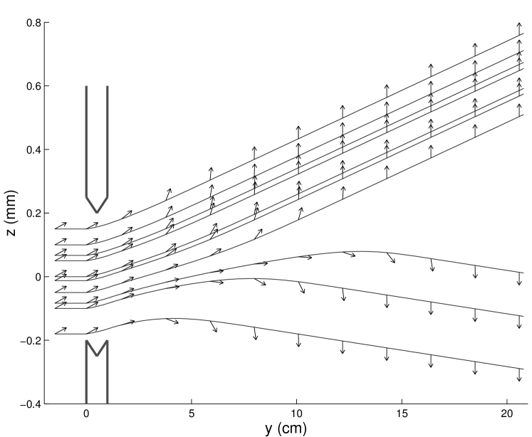
Figure 12: Ten silver atom trajectories with initial spin orientation $(\theta_{0}=\frac{\pi}{3})$ and initial position $z_{0}$; arrows represent the spin orientation $\theta(z,t)$ along the trajectories.

The final orientation, obtained after the decoherence time $t_{D}$, depends on the initial particle position $z_{0}$ in the spinor with a spatial extension and on the initial angle $\theta_{0}$ of the spin with the $z$-axis. We obtain $+\frac{\pi}{2}$ if $z_{0}>z^{\theta_{0}}$ and $-\frac{\pi}{2}$ if $z_{0}<z^{\theta_{0}}$ with

$$z^{\theta_{0}}=\sigma_{0}F^{-1}\left(\sin^{2}\frac{\theta_{0}}{2}\right)$$ (26)

where F is the repartition function of the normal centered-reduced law. If we ignore the position of the atom in its wave function, we lose the determinism given by equation (26).

In the de Broglie-Bohm interpretation with a realistic interpretation of the spin, the "measured" value is not independent of the context of the measure and is contextual. It conforms to the Kochen and Specker theorem: Kochen 1967 Realism and non-contextuality are inconsistent with certain quantum mechanics predictions.

Now let us consider a mixture of pure states where the initial orientation ($\theta_{0},\varphi_{0}$) from the spinor has been randomly chosen. These are the conditions of the initial Stern and Gerlach experiment. Figure 13 represents a simulation of 10 quantum trajectories of silver atoms from which the initial positions $z_{0}$ are also randomly chosen.

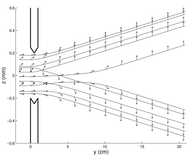
Figure 13: Ten silver atom trajectories where the initial orientation ($\theta_{0},\varphi_{0}$) has been randomly chosen; arrows represent the spin orientation $\theta(z,t)$ along the trajectories.

Finally, the de Broglie-Bohm trajectories propose a clear interpretation of the spin measurement in quantum mechanics. There is interaction with the measuring apparatus as is generally stated; and there is indeed a minimum time required to measure. However this measurement and this time do not have the signification that is usually applied to them. The result of the Stern-Gerlach experiment is not the measure of the spin projection along the $z$-axis, but the orientation of the spin either in the direction of the magnetic field gradient, or in the opposite direction. It depends on the position of the particle in the wave function. We have therefore a simple explanation for the non-compatibility of spin measurements along different axes. The measurement duration is then the time necessary for the particle to point its spin in the final direction.

V EPR-B experiment

Nonseparability is one of the most puzzling aspects of quantum mechanics. For over thirty years, the EPR-B, the spin version of the Einstein-Podolsky-Rosen experiment EPR proposed by Bohm Bohm_1951 , the Bell theorem Bell64 and the BCHSH inequalities Bell64 ; BCHSH ; Bell_1987 have been at the heart of the debate on hidden variables and non-locality. Many experiments since Bell’s paper have demonstrated violations of these inequalities and have vindicated quantum theory Clauser_1972 . Now, EPR pairs of massive atoms are also considered Beige . The usual conclusion of these experiments is to reject the non-local realism for two reasons: the impossibility of decomposing a pair of entangled atoms into two states, one for each atom, and the impossibility of interaction faster than the speed of light.

Here, we show that there exists a de Broglie-Bohm interpretation which answers these two questions positively. To demonstrate this non-local realism, two methodological conditions are necessary. The first condition is the same as in the Stern-Gerlach experiment: the solution to the entangled state is obtained by resolving the Pauli equation from an initial singlet wave function with a spatial extension as:

$$\Psi_{0}(\textbf{r}_{A},\textbf{r}_{B})=\frac{1}{\sqrt{2}}f(\textbf{r}_{A})f(\textbf{r}_{B})(|+_{A}\rangle|-_{B}\rangle-|-_{A}\rangle|+_{B}\rangle),$$ (27)

and not from a simplified wave function without spatial extension:

$$\Psi_{0}(\textbf{r}_{A},\textbf{r}_{B})=\frac{1}{\sqrt{2}}(|+_{A}\rangle|-_{B}\rangle-|-_{A}\rangle|+_{B}\rangle).$$ (28)

$f$ function and $|\pm\rangle$ vectors are presented later.

The resolution in space of the Pauli equation is essential: it enables the spin measurement by spatial quantization and explains the determinism and the disentangling process. To explain the interaction and the evolution between the spin of the two particles, we consider a two-step version of the EPR-B experiment. It is our second methodological condition. A first causal interpretation of EPR-B experiment was proposed in 1987 by Dewdney, Holland and Kyprianidis Dewdney_1987b using these two conditions. However, this interpretation had a flaw Holland_1993 (p. 418): the spin module of each particle depends directly on the singlet wave function, and thus the spin module of each particle varied during the experiment from 0 to $\frac{\hbar}{2}$. We present a de Broglie-Bohm interpretation that avoid this flaw. Gondran_2012

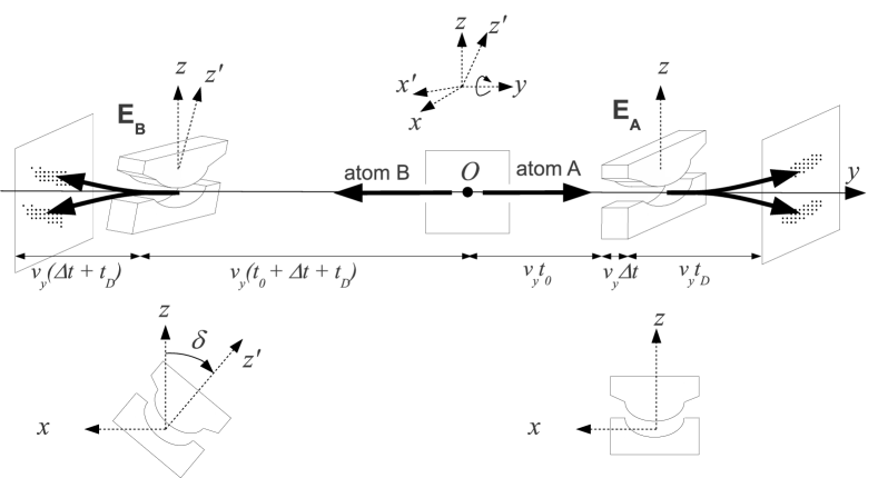
Figure 14: Schematic configuration of the EPR-B experiment.

Figure 14 presents the Einstein-Podolsky-Rosen-Bohm experiment. A source $S$ created in O pairs of identical atoms A and B, but with opposite spins. The atoms A and B split following the $y$-axis in opposite directions, and head towards two identical Stern-Gerlach apparatus $\textbf{E}_{\textbf{A}}$ and $\textbf{E}_{\textbf{B}}$. The electromagnet $\textbf{E}_{\textbf{A}}$ "measures" the spin of A along the $z$-axis and the electromagnet $\textbf{E}_{\textbf{B}}$ "measures" the spin of B along the $z^{\prime}$-axis, which is obtained after a rotation of an angle $\delta$ around the $y$-axis. The initial wave function of the entangled state is the singlet state (27) where $\textbf{r}=(x,z)$, $f(\textbf{r})=(2\pi\sigma_{0}^{2})^{-\frac{1}{2}}e^{-\frac{x^{2}+z^{2}}{4\sigma_{0}^{2}}}$, $|\pm_{A}\rangle$ and $|\pm_{B}\rangle$ are the eigenvectors of the operators $\sigma_{z_{A}}$ and $\sigma_{z_{B}}$: $\sigma_{z_{A}}|\pm_{A}\rangle=\pm|\pm_{A}\rangle$, $\sigma_{z_{B}}|\pm_{B}\rangle=\pm|\pm_{B}\rangle$. We treat the dependence with $y$ classically: speed $-v_{y}$ for A and $v_{y}$ for B. The wave function $\Psi(\textbf{r}_{A},\textbf{r}_{B},t)$ of the two identical particles A and B, electrically neutral and with magnetic moments $\mu_{0}$, subject to magnetic fields ${\textbf{E}_{\textbf{A}}}$ and ${\textbf{E}_{\textbf{B}}}$, admits on the basis of $|\pm_{A}\rangle$ and $|\pm_{B}\rangle$ four components $\Psi^{a,b}(\textbf{r}_{A},\textbf{r}_{B},t)$ and satisfies the two-body Pauli equation Holland_1993 (p. 417):

$$i\hbar\frac{\partial\Psi^{a,b}}{\partial t}= \left(-\frac{\hbar^{2}}{2m}\Delta_{A}-\frac{\hbar^{2}}{2m}\Delta_{B}\right)\Psi^{a,b}$$ (29)

$$+ \mu B^{\textbf{E}_{\textbf{A}}}_{j}(\sigma_{j})_{c}^{a}\Psi^{c,b}+\mu B^{\textbf{E}_{\textbf{B}}}_{j}(\sigma_{j})_{d}^{b}\Psi^{a,d}$$

with the initial conditions:

$$\Psi^{a,b}(\textbf{r}_{A},\textbf{r}_{B},0)=\Psi_{0}^{a,b}(\textbf{r}_{A},\textbf{r}_{B})$$ (30)

where $\Psi_{0}^{a,b}(\textbf{r}_{A},\textbf{r}_{B})$ corresponds to the singlet state (27).

To obtain an explicit solution of the EPR-B experiment, we take the numerical values of the Stern-Gerlach experiment.

One of the difficulties of the interpretation of the EPR-B experiment is the existence of two simultaneous measurements. By doing these measurements one after the other, the interpretation of the experiment will be facilitated. That is the purpose of the two-step version of the experiment EPR-B studied below.

V.1 First step EPR-B: Spin measurement of A

In the first step we make a Stern and Gerlach "measurement" for atom A, on a pair of particles A and B in a singlet state. This is the experiment first proposed in 1987 by Dewdney, Holland and Kyprianidis. Dewdney_1987b

Consider that at time $t_{0}$ the particle A arrives at the entrance of electromagnet $\textbf{E}_{\textbf{A}}$. After this exit of the magnetic field $\textbf{E}_{\textbf{A}}$, at time $t_{0}+\triangle t+t$, the wave function (27) becomes Gondran_2012 :

$$\Psi(\textbf{r}_{A},\textbf{r}_{B},t_{0}+\triangle t+t)=\frac{1}{\sqrt{2}}f(\textbf{r}_{B})\times( f^{+}(\textbf{r}_{A},t)|+_{A}\rangle|-_{B}\rangle$$

$$- f^{-}(\textbf{r}_{A},t)|-_{A}\rangle|+_{B}\rangle)$$

with

$$f^{\pm}(\textbf{r},t)\simeq f(x,z\mp z_{\triangle}\mp ut)e^{i(\frac{\pm muz}{\hbar}+\varphi^{\pm}(t))}$$ (32)

where $z_{\Delta}$ and $u$ are given by equation (21).

The atomic density $\rho(z_{A},z_{B},t_{0}+\Delta t+t)$ is found by integrating $\Psi^{*}(\textbf{r}_{A},\textbf{r}_{B},t_{0}+\triangle t+t)\Psi(\textbf{r}_{A},\textbf{r}_{B},t_{0}+\triangle t+t)$ on $x_{A}$ and $x_{B}$:

$$\rho (z_{A} ,z_{B},t_{0}+\Delta t+t)=\left((2\pi\sigma_{0}^{2})^{-\frac{1}{2}}e^{-\frac{(z_{B})^{2}}{2\sigma_{0}^{2}}}\right)$$

$$\times \left((2\pi\sigma_{0}^{2})^{-\frac{1}{2}}\frac{1}{2}\left(e^{-\frac{(z_{A}-z_{\Delta}-ut)^{2}}{2\sigma_{0}^{2}}}+e^{-\frac{(z_{A}+z_{\Delta}+ut)^{2}}{2\sigma_{0}^{2}}}\right)\right).$$

We deduce that the beam of particle A is divided into two, while the beam of particle B stays undivided:

• the density of A is the same, whether particle A is entangled with B or not,

• the density of B is not affected by the "measurement" of A.

Our first conclusion is: the position of B does not depend on the measurement of A, only the spins are involved. We conclude from equation (LABEL:eq:7psiexperience1) that the spins of A and B remain opposite throughout the experiment. These are the two properties used in the causal interpretation.

V.2 Second step EPR-B: Spin measurement of B

The second step is a continuation of the first and corresponds to the EPR-B experiment broken down into two steps. On a pair of particles A and B in a singlet state, first we made a Stern and Gerlach measurement on the A atom between $t_{0}$ and $t_{0}+\triangle t+t_{D}$, secondly, we make a Stern and Gerlach measurement on the B atom with an electromagnet $\textbf{E}_{\textbf{B}}$ forming an angle $\delta$ with $\textbf{E}_{\textbf{A}}$ during $t_{0}+\triangle t+t_{D}$ and $t_{0}+2(\triangle t+t_{D})$.

At the exit of magnetic field $\textbf{E}_{\textbf{A}}$, at time $t_{0}+\triangle t+t_{D}$, the wave function is given by (LABEL:eq:7psiexperience1). Immediately after the measurement of A, still at time $t_{0}+\triangle t+t_{D}$, the wave function of B depends on the measurement $\pm$ of A:

$$\Psi_{B/\pm A}(\textbf{r}_{B},t_{0}+\triangle t+t_{1})=f(\textbf{r}_{B})|\mp_{B}\rangle.$$ (34)

Then, the measurement of B at time $t_{0}+2(\triangle t+t_{D})$ yields, in this two-step version of the EPR-B experiment, the same results for spatial quantization and correlations of spins as in the EPR-B experiment.

V.3 Causal interpretation of the EPR-B experiment

We assume, at the creation of the two entangled particles A and B, that each of the two particles A and B has an initial wave function with opposite spins: $\Psi_{0}^{A}(\textbf{r}_{A},\theta^{A}_{0},\varphi^{A}_{0})=f(\textbf{r}_{A})\left(\cos\frac{\theta^{A}_{0}}{2}|+_{A}\rangle+\sin\frac{\theta^{A}_{0}}{2}e^{i\varphi^{A}_{0}}|-_{A}\rangle\right)$ and $\Psi_{0}^{B}(\textbf{r}_{B},\theta^{B}_{0},\varphi^{B}_{0})=f(\textbf{r}_{B})\left(\cos\frac{\theta^{B}_{0}}{2}|+_{B}\rangle+\sin\frac{\theta^{B}_{0}}{2}e^{i\varphi^{B}_{0}}|-_{B}\rangle\right)$ with $\theta_{0}^{B}=\pi-\theta_{0}^{A}$ and $\varphi_{0}^{B}=\varphi_{0}^{A}-\pi$. The two particles A and B are statistically prepared as in the Stern and Gerlach experiment. Then the Pauli principle tells us that the two-body wave function must be antisymmetric; after calculation we find the same singlet state (27):

$$\Psi_{0}(\textbf{r}_{A},\theta^{A},\varphi^{A},\textbf{r}_{B},\theta^{B},\varphi^{B})= - e^{i\varphi^{A}}f(\textbf{r}_{A})f(\textbf{r}_{B})$$

$$\times \left(|+_{A}\rangle|-_{B}\rangle-|-_{A}\rangle|+_{B}\rangle\right).$$

Thus, we can consider that the singlet wave function is the wave function of a family of two fermions A and B with opposite spins: the direction of initial spin A and B exists, but is not known. It is a local hidden variable which is therefore necessary to add in the initial conditions of the model.

This is not the interpretation followed by the Bohm school Dewdney_1987b ; Dewdney_1986 ; Bohm_1993 ; Holland_1993 in the interpretation of the singlet wave function; they do not assume the existance of wave functions $\Psi_{0}^{A}(\textbf{r}_{A},\theta^{A}_{0},\varphi^{A}_{0})$ and $\Psi_{0}^{B}(\textbf{r}_{B},\theta^{B}_{0},\varphi^{B}_{0})$ for each particle, but only the singlet state $\Psi_{0}(\textbf{r}_{A},\theta^{A},\varphi^{A},\textbf{r}_{B},\theta^{B},\varphi^{B})$. In consequence, they suppose a zero spin for each particle at the initial time and a spin module of each particle varied during the experiment from 0 to $\frac{\hbar}{2}$ Holland_1993 (p. 418).

Here, we assume that at the initial time we know the spin of each particle (given by each initial wave function) and the initial position of each particle.

Step 1: spin measurement of A

In the equation (LABEL:eq:7psiexperience1) particle A can be considered independent of B. We can therefore give it the wave function

$$\Psi^{A}(\textbf{r}_{A},t_{0}+\triangle t+t)= \cos\frac{\theta_{0}^{A}}{2}f^{+}(\textbf{r}_{A},t)|+_{A}\rangle$$ (36)

$$+\sin\frac{\theta_{0}^{A}}{2}e^{i\varphi_{0}^{A}}f^{-}(\textbf{r}_{A},t)|-_{A}\rangle$$

which is the wave function of a free particle in a Stern Gerlach apparatus and whose initial spin is given by ($\theta_{0}^{A},\varphi_{0}^{A}$). For an initial polarization ($\theta_{0}^{A},\varphi_{0}^{A}$) and an initial position ($z_{0}^{A}$), we obtain, in the de Broglie-Bohm interpretation Bohm_1993 of the Stern and Gerlach experiment, an evolution of the position ($z_{A}(t)$) and of the spin orientation of A ($\theta^{A}(z_{A}(t),t)$) Gondran_2005b .

The case of particle B is different. B follows a rectilinear trajectory with $y_{B}(t)=v_{y}t$, $z_{B}(t)=z_{0}^{B}$ and $x_{B}(t)=x_{0}^{B}$. By contrast, the orientation of its spin moves with the orientation of the spin of A: $\theta^{B}(t)=\pi-\theta^{A}(z_{A}(t),t)$ and $\varphi^{B}(t)=\varphi(z_{A}(t),t)-\pi$. We can then associate the wave function:

$$\Psi^{B}(\textbf{r}_{B},t_{0}+\triangle t+t)=f(\textbf{r}_{B}) \left(\cos\frac{\theta^{B}(t)}{2}|+_{B}\rangle\right.$$

$$\quad\left.+\sin\frac{\theta^{B}(t)}{2}e^{i\varphi^{B}(t)}|-_{B}\rangle\right).$$

This wave function is specific, because it depends upon initial conditions of A (position and spin). The orientation of spin of the particle B is driven by the particle A through the singlet wave function. Thus, the singlet wave function is the non-local variable.

Step 2: Spin measurement of B

At the time $t_{0}+\Delta t+t_{D}$, immediately after the measurement of A, $\theta^{B}(t_{0}+\Delta t+t_{D})=\pi$ or 0 in accordance with the value of $\theta^{A}(z_{A}(t),t)$ and the wave function of B is given by (34). The frame $(Ox^{\prime}yz^{\prime})$ corresponds to the frame $(Oxyz)$ after a rotation of an angle $\delta$ around the $y$-axis. $\theta^{B}$ corresponds to the B-spin angle with the $z$-axis, and $\theta^{\prime B}$ to the B-spin angle with the $z^{\prime}$-axis, then $\theta^{\prime B}(t_{0}+\Delta t+t_{D})=\pi+\delta$ or $\delta$. In this second step, we are exactly in the case of a particle in a simple Stern and Gerlach experiment (with magnet $\textbf{E}_{\textbf{B}}$) with a specific initial polarization equal to $\pi+\delta$ or $\delta$ and not random like in step 1. Then, the measurement of B, at time $t_{0}+2(\triangle t+t_{D})$), gives, in this interpretation of the two-step version of the EPR-B experiment, the same results as in the EPR-B experiment.

V.4 Physical explanation of non-local influences

From the wave function of two entangled particles, we find spins, trajectories and also a wave function for each of the two particles. In this interpretation, the quantum particle has a local position like a classical particle, but it has also a non-local behavior through the wave function. So, it is the wave function that creates the non classical properties. We can keep a view of a local realist world for the particle, but we should add a non-local vision through the wave function. As we saw in step 1, the non-local influences in the EPR-B experiment only concern the spin orientation, not the motion of the particles themselves. Indeed only spins are entangled in the wave function (27) not positions and motions like in the initial EPR experiment. This is a key point in the search for a physical explanation of non-local influences.

The simplest explanation of this non-local influence is to reintroduce the concept of ether (or the preferred frame), but a new format given by Lorentz-Poincaré and by Einstein in 1920Einstein_1920 : "Recapitulating, we may say that according to the general theory of relativity space is endowed with physical qualities; in this sense, therefore, there exists an ether. According to the general theory of relativity space without ether is unthinkable; for in such space there not only would be no propagation of light, but also no possibility of existence for standards of space and time (measuring-rods and clocks), nor therefore any space-time intervals in the physical sense. But this ether may not be thought of as endowed with the quality characteristic of ponderable media, as consisting of parts which may be tracked through time. The idea of motion may not be applied to it."

Taking into account the new experiments, especially Aspect’s experiments, Popper Popper_1982 (p. XVIII) defends a similar view in 1982:

"I feel not quite convinced that the experiments are correctly interpreted; but if they are, we just have to accept action at a distance. I think (with J.P. Vigier) that this would of course be very important, but I do not for a moment think that it would shake, or even touch, realism. Newton and Lorentz were realists and accepted action at a distance; and Aspect’s experiments would be the first crucial experiment between Lorentz’s and Einstein’s interpretation of the Lorentz transformations."

Finally, in the de Broglie-Bohm interpretation, the EPR-B experiments of non-locality have therefore a great importance, not to eliminate realism and determinism, but as Popper said, to rehabilitate the existence of a certain type of ether, like Lorentz’s ether and like Einstein’s ether in 1920.

VI Conclusion

In the three experiments presented in this article, the variable that is measured in fine is the position of the particle given by this impact on a screen. In the double-slit, the set of these positions gives the interferences; in the Stern-Gerlach and the EPR-B experiments, it is the position of the particle impact that defines the spin value.

It is this position that the de Broglie-Bohm interpretation adds to the wave function to define a complete state of the quantum particle. The de Broglie-Bohm interpretation is then based only on the initial conditions $\Psi^{0}(x)$ and $X(0)$ and the evolution equations (1) and (12). If we add as initial condition the "quantum equilibrium hypothesis" (14), we have seen that we can deduce, for these three examples, the three postulates of measurement. These three postulates are not necessary if we solve the time-dependent Schrödinger equation (double-slit experiment) or the Pauli equation with spatial extension (Stern-Gerlach and EPR experiments). However, these simulations enable us to better understand those experiments: In the double-slit experiment, the interference phenomena appears only some centimeters after the slits and shows the continuity with classical mechanics; in the Stern-Gerlach experiment, the spin up/down measurement appears also after a given time, called decoherence time; in the EPR-B experiment, only the spin of B is affected by the spin measurement of A, not its density. Moreover, the de Broglie-Bohm trajectories propose a clear explanation of the spin measurement in quantum mechanics.

However, we have seen two very different cases in the measurement process. In the first case (double slit experiment), there is no influence of the measuring apparatus (the screen) on the quantum particle. In the second case (Stern-Gerlach experiment, EPR-B), there is an interaction with the measuring apparatus (the magnetic field) and the quantum particle. The result of the measurement depends on the position of the particle in the wave function. The measurement duration is then the time necessary for the stabilisation of the result.

This heterodox interpretation clearly explains experiments with a set of quantum particles that are statistically prepared. These particles verify the "quantum equilibrium hypothesis" and the de Broglie-Bohm interpretation establishes continuity with classical mechanics. However, there is no reason that the de Broglie-Bohm interpretation can be extended to quantum particles that are not statistically prepared. This situation occurs when the wave packet corresponds to a quasi-classical coherent state, introduced in 1926 by Schrödinger Schrodinger_26 . The field quantum theory and the second quantification are built on these coherent states Glauber_65 . It is also the case, for the hydrogen atom, of localized wave packets whose motion are on the classical trajectory (an old dream of Schrödinger’s). Their existence was predicted in 1994 by Bialynicki-Birula, Kalinski, Eberly, Buchleitner and Delande Bialynicki_1994 ; Delande_1995 ; Delande_2002 , and discovered recently by Maeda and Gallagher Gallagher on Rydberg atoms. For these non statistically prepared quantum particles, we have shown Gondran2011 ; Gondran2012a that the natural interpetation is the Schrödinger interpretation proposed at the Solvay congress in 1927. Everythings happens as if the quantum mechanics interpretation depended on the preparation of the particles (statistically or not statistically prepared). It is perhaps a response to the "theory of the double solution" that Louis de Broglie was seeking since 1927: "I introduced as the "double solution theory" the idea that it was necessary to distinguish two different solutions that are both linked to the wave equation, one that I called wave $u$, which was a real physical wave represented by a singularity as it was not normalizable due to a local anomaly defining the particle, the other one as Schrödinger’s $\Psi$ wave, which is a probability representation as it is normalizable without singularities." Broglie

Appendix A Calculating the spinor evolution in the Stern-Gerlach experiment

In the magnetic field $B=(B_{x},0,B_{z})$, the Pauli equation (18) gives coupled Schrödinger equations for each spinor component

$$i\hbar\frac{\partial\psi_{\pm}}{\partial t}(x,z,t)= - \frac{\hbar^{2}}{2m}\nabla^{2}\psi_{\pm}(x,z,t)$$ (38)

$$\pm \mu_{B}(B_{0}-B_{0}^{\prime}z)\psi_{\pm}(x,z,t)$$

$$\mp i\mu_{B}B_{0}^{\prime}x\psi_{\mp}(x,z,t).$$

If one effects the transformation Platt_1992

$$\psi_{\pm}(x,z,t)=\exp\left(\pm\frac{i\mu_{B}B_{0}t}{\hbar}\right)\overline{\psi}_{\pm}(x,z,t)$$

equation (38) becomes

$$i\hbar\frac{\partial\overline{\psi}_{\pm}}{\partial t}(x,z,t)= - \frac{\hbar^{2}}{2m}\nabla^{2}\overline{\psi}_{\pm}(x,z,t)$$

$$\mp \mu_{B}B^{\prime}_{0}z\overline{\psi}_{\pm}(x,z,t)$$

$$\mp i\mu_{B}B^{\prime}_{0}x\overline{\psi}_{\mp}(x,z,t)\exp\left(\pm i\frac{2\mu_{B}B_{0}t}{\hbar}\right)$$

The coupling term oscillates rapidly with the Larmor frequency $\omega_{L}=\frac{2\mu_{B}B_{0}}{\hbar}=1,4\times 10^{11}s^{-1}$. Since $|B_{0}|\gg|B^{\prime}_{0}z|$ and $|B_{0}|\gg|B^{\prime}_{0}x|$, the period of oscillation is short compared to the motion of the wave function. Averaging over a period that is long compared to the oscillation period, the coupling term vanishes, which entailsPlatt_1992

$$i\hbar\frac{\partial\overline{\psi}_{\pm}}{\partial t}(x,z,t)=-\frac{\hbar^{2}}{2m}\nabla^{2}\overline{\psi}_{\pm}(x,z,t)\mp\mu_{B}B^{\prime}_{0}z\overline{\psi}_{\pm}(x,z,t).$$ (39)

Since the variable x is not involved in this equation and $\psi^{0}_{\pm}(x,z)$ does not depend on x, $\overline{\psi_{\pm}}(x,z,t)$ does not depend on x: $\overline{\psi_{\pm}}(x,z,t)\equiv\overline{\psi_{\pm}}(z,t)$. Then we can explicitly compute the preceding equations for all t in $[0,\Delta t]$ with $\Delta t=\frac{\Delta l}{v}=2\times 10^{5}s$.

We obtain:

$$\overline{\psi}_{+}(z,t)=\psi_{K}(z,t)\cos\frac{\theta_{0}}{2}e^{i\frac{\varphi_{0}}{2}}~{}~{}~{} ~{}~{}\text{and}~{}~{}K=-\mu_{B}B^{\prime}_{0}$$

$$\overline{\psi}_{-}(z,t)=\psi_{K}(z,t)i\sin\frac{\theta_{0}}{2}e^{-i\frac{\varphi_{0}}{2}} ~{}~{}\text{and}~{}~{}K=+\mu_{B}B^{\prime}_{0}$$

$\sigma_{t}^{2}=\sigma_{0}^{2}+\left(\frac{\hbar t}{2m\sigma_{0}}\right)^{2}$ and

$$\psi_{K}(z,t) = (2\pi\sigma_{t}^{2})^{-\frac{1}{4}}e^{-\frac{(z+\frac{Kt^{2}}{2m})^{2}}{4\sigma_{t}^{2}}}\exp\frac{i}{\hbar}\left[-\frac{\hbar}{2}\tan^{-1}\left(\frac{\hbar t}{2m\sigma_{0}^{2}}\right)\right.$$ (40)

$$\left.-Ktz-\frac{K^{2}t^{3}}{6m}+\frac{(z+\frac{Kt^{2}}{2m})^{2}\hbar^{2}t^{2}}{8m\sigma_{0}^{2}\sigma_{t}^{2}}\right].$$

where (40) is a classical result.Feynman

The experimental conditions give $\frac{\hbar\Delta t}{2m\sigma_{0}}=4\times 10^{-11}~{}m\ll\sigma_{0}=10^{-4}~{}m$. We deduce the approximations $\sigma_{t}\simeq\sigma_{0}$ and

$$\overline{\psi}_{K}(z,t)\simeq(2\pi\sigma_{0}^{2})^{-\frac{1}{4}}e^{-\frac{(z+\frac{Kt^{2}}{2m})^{2}}{4\sigma_{0}^{2}}}\exp\frac{i}{\hbar}\left[-Ktz-\frac{K^{2}t^{3}}{6m}\right].$$ (41)

At the end of the magnetic field, at time $\Delta t$, the spinor equals to

$$\Psi(z,\Delta t)=\left(\begin{array}[]{c}\psi_{+}(z,\Delta t)\\ \psi_{-}(z,\Delta t)\end{array}\right)$$ (42)

with

$$\psi_{+}(z,\Delta t) = (2\pi\sigma_{0}^{2})^{-\frac{1}{4}}e^{-\frac{(z-z_{\Delta})^{2}}{4\sigma_{0}^{2}}+\frac{i}{\hbar}muz}\cos\frac{\theta_{0}}{2}e^{i\varphi_{+}}$$

$$\psi_{-}(z,\Delta t) = (2\pi\sigma_{0}^{2})^{-\frac{1}{4}}e^{-\frac{(z+z_{\Delta})^{2}}{4\sigma_{0}^{2}}-\frac{i}{\hbar}muz}i\sin\frac{\theta_{0}}{2}e^{i\varphi_{-}}$$

$$z_{\Delta} =\frac{\mu_{B}B^{\prime}_{0}(\Delta t)^{2}}{2m},~{}~{}~{}~{}~{}~{}u=\frac{\mu_{0}B^{\prime}_{0}(\Delta t)}{m}~{}~{}~{}~{}\text{and}$$

$$\varphi_{+} =\frac{\varphi_{0}}{2}-\frac{\mu_{B}B_{0}\Delta t}{\hbar}-\frac{K^{2}(\Delta t)^{3}}{6m\hbar};$$

$$\varphi_{-} =-\frac{\varphi_{0}}{2}+\frac{\mu_{0}B_{0}\Delta t}{\hbar}-\frac{K^{2}(\Delta t)^{3}}{6m\hbar}.$$

We remark that the passage through the magnetic field gives the equivalent of a velocity $+u$ in the direction $0z$ to the function $\psi_{+}$ and a velocity $-u$ to the function $\psi_{-}$. Then we have a free particle with the initial wave function (42). The Pauli equation resolution again yields $\psi_{\pm}(x,z,t)=\psi_{x}(x,t)\psi_{\pm}(z,t)$ and with the experimental conditions we have $\psi_{x}(x,t)\simeq(2\pi\sigma_{0}^{2})^{-\frac{1}{4}}e^{-\frac{x^{2}}{4\sigma_{0}^{2}}}$ and

$$\psi_{+}(z,t+\Delta t) \simeq (2\pi\sigma_{0}^{2})^{-\frac{1}{4}}\cos\frac{\theta_{0}}{2}$$

$$\times\exp^{-\frac{(z-z_{\Delta}-ut)^{2}}{4\sigma_{0}^{2}}+\frac{i}{\hbar}(muz-\frac{1}{2}mu^{2}t+\hbar\varphi_{+})}$$

$$\psi_{-}(z,t+\Delta t) \simeq (2\pi\sigma_{0}^{2})^{-\frac{1}{4}}i\sin\frac{\theta_{0}}{2}$$

$$\times\exp^{-\frac{(z+z_{\Delta}+ut)^{2}}{4\sigma_{0}^{2}}+\frac{i}{\hbar}(-muz-\frac{1}{2}mu^{2}t+\hbar\varphi_{-})}$$

References

- (1) J. S. Bell, "On the impossible pilot wave", 1982, reprint in Bell 1987, in Speakable and Unspeakable in Quantum Mechanics (Cambridge University Press, 1987).
- (2) D. Bohm, "A suggested interpretation of the quantum theory in terms of hidden variables, I and II", Phys. Rev. 85, 166-193 (1952).
- (3) J. von Neumann, Mathematical Foundations of Quantum Mechanics (Princeton Univ. Press, 1996).
- (4) B. d’Espagnat, A la recherche du réel (Gauthiers-Villard, Paris, 1979).
- (5) J. S. Bell, Speakable and Unspeakable in Quantum Mechanics (Cambridge University Press, 1987), 2nd edition, 2004.
- (6) L. de Broglie, "La mécanique ondulatoire et la structure atomique de la matière et du rayonnement," J. de Phys. 8, 225-241 (1927). An English translation can be found in G. Bacciagalluppi and A. Valentini, Quantum Theory of the Crossroads (Cambridge University Press, Cambridge, 2009)
- (7) Madelung, E.: Quantentheorie in hydrodynamischer Form. Zeit. Phys. 40, 322-6 (1926).
- (8) M. Gondran and A. Gondran, "Discerned and non-discerned particles in classical mechanics and convergence of quantum mechanics to classical mechanics", Annales de la Fondation Louis de Broglie, vol. 36, 117-135 (2011).
- (9) M. Gondran, and A. Gondran, "The two limits of the Schrödinger equation in the semi-classical approximation : discerned and non-discerned particles in classical mechanics", Foundations of Probability and Physics-6, AIP Conf. Proc. 1424,111-115 (2012).
- (10) R. Feynman and A. Hibbs, Quantum Mechanics and Paths Integrals (McGraw-Hill, Inc., 1965), pp.63.
- (11) C. Cohen-Tannoudji, B. Diu, and F. Laloë, Quantum Mechanics (Wiley, New York, 1977).
- (12) D. Dürr, S. Golstein, and N. Zanghi, "Quantum equilibrium and the origin of absolute uncertainty," J. Stat. Phys. 67, 843-907 (1992).
- (13) A. S. Sanz and S. Miret-Artès, "Quantum phase analysis with quantum trajectories: A step towards the creation of a Bohmian thinking", Am. J. Phys. 80, 525 (2012).
- (14) T. Norsen, "The pilot-wave perspective on quantum scattering and tunneling", Am. J. Phys. 81, 258-266 (2013).
- (15) C. Jönsson, “Elektroneninterferenzen an mehreren künstlich hergestellten Feinspalten,” Z. Phy. 161, 454–474 (1961), English translation “Electron diffraction at multiple slits,” Am. J. Phys. 42, 4–11 (1974).
- (16) T. Young, "On the theory of light and colors,” Philos. Trans. RSL 92, 12–48 (1802).
- (17) C. J. Davisson and L. H. Germer, “The scattering of electrons by a single crystal of nickel,” Nature 119, 558–560 (1927). P. G. Merlin, C. F. Missiroli, and G. Pozzi, “On the statistical aspect of electron interference phenomena,” Am. J. Phys. 44, 306–307 (1976). A. Tonomura, J. Endo, T. Matsuda, T. Kawasaki, and H. Ezawa, “Demonstration of single-electron buildup of an interference pattern,” Am. J. Phys. 57, 117–120 (1989).
- (18) H. V. Halbon Jr. and P. Preiswerk, “Preuve expérimentale de la diffraction des neutrons,” C. R. Acad. Sci. Paris 203, 73–75 (1936). H. Rauch and A. Werner, Neutron Interferometry: Lessons in Experimental Quantum Mechanics (Oxford Univ. Press, London, 2000).
- (19) A. Zeilinger, R. Gähler, C. G. Shull, W. Treimer, and W. Mampe, “Single and double slit diffraction of neutrons,” Rev. Mod. Phys. 60, 1067–1073 (1988).
- (20) I. Estermann and O. Stern,“Beugung von Molekularstrahlen,” Z. Phy. 61, 95–125 (1930).
- (21) F. Shimizu, K. Shimizu, and H. Takuma, “Double-slit interference with ultracold metastable neon atoms,” Phys. Rev. A 46, R17–R20 (1992). M. H. Anderson, J. R. Ensher, M. R. Mattheus, C. E. Wieman, and E. A. Cornell, “Observation of Bose-Einstein condensation in a dilute atomic vapor,” Science 269, 198–201 (1995).
- (22) M. Arndt, O. Nairz, J. Voss-Andreae, C. Keller, G. van des Zouw, and A. Zeilinger, “Wave-particle duality of C60 molecules,” Nature 401, 680–682 (1999). O. Nairz, M. Arndt, and A. Zeilinger, “Experimental challenges in fullerene interferometry,” J. Mod. Opt. 47, 2811–2821 (2000).
- (23) R. P. Feynman, R. B. Leighton, and M. Sands, The Feynman Lectures on Physics (Addison-Wesley, New York, 1965).
- (24) M. Gondran, A. Gondran, "Numerical simulation of the double-slit interference with ultracold atoms", Am. J. Phys. 73, 6 (2005).
- (25) C. Philippidis, C. Dewdney, and B. J. Hiley, "Quantum interference and the quantum potential", Il Nuovo Cimento 52 B, 15-28 (1979).
- (26) W. Gerlach and O. Stern,"Der Experimentelle Nachweis des Magnetischen Moments des Silberatoms", Zeit. Phys. 8, 110 (1921); Zeit. Phys. 9, 349 (1922).
- (27) H. D. Zeh, "On the Interpretation of Measurement in Quantum Theory," Found. Phys.1, 69-76 (1970). Reprinted in Wheeler and Zurek (1983), pp. 342-349. W. H. Zurek, "Environment-Induced Superselection Rules", Phys.Rev.D26 1862 (1982) ; J.A. Wheeler, and W. H. Zurek, Quantum Theory of Measurement (Princeton University Press, 1983); W. H. Zurek, "Decoherence, einselection and the quantum origins of the classical", Rev. Mod. Phys. 75 (2003) 715. R. Omnes, "Consistent Interpretation of Quantum Mechanics", Rev. Mod. Phys. 64, 339 (1992). M. Schlosshauer, Decoherence and the Quantum-to-Classical Transition (Springer-Verlag, 2007).
- (28) J.J. Sakurai, Modern Quantum Mechanics (Addison-Wesley, 1985).
- (29) M. Le Bellac, Quantum Physics (Cambridge University Press, 2006).
- (30) T.Takabayasi, "On the Formulation of Quantum Mechanics associated with Classical Pictures", Prog. Theor. Phys., 8 2, 143 (1952); "The Formulation of Quantum Mechanics in terms of Ensemble in Phase Space", Prog. Theor. Phys., 11 4-5, 341 (1954).
- (31) D. Bohm, R. Schiller,and J. Tiomno, "A causal interpretation of the pauli equation", Nuovo Cim. supp. 1, 48-66 and 67-91(1955).
- (32) D. Bohm,and B.J. Hiley, The Undivided Universe (Routledge, London and New York, 1993).
- (33) C. Dewdney, P.R. Holland, and A. Kypianidis, "What happens in a spin measurement?", Phys. Lett. A, 119(6), 259-267 (1986).
- (34) P.R. Holland , The Quantum Theory of Motion (Cambridge University Press, 1993).
- (35) C. Dewdney, P.R. Holland, and A. Kyprianidis, "A causal account of non-local Einstein-Podolsky-Rosen spin correlations," J. Phys. A, Math. Gen. 20, 4717-32 (1987). C. Dewdney, P.R. Holland, A. Kyprianidis, and J.P. Vigier, "Spin and non-locality in quantum mechanics," Nature, 336, 536-44 (1988).
- (36) M. Gondran, A. Gondran, "A new causal interpretation of EPR-B experiment," Quantum Theory: Reconsideration of Foundations 6, AIP Conf. Proc. 1508, 370-375 (2012).
- (37) D.E. Platt, "A modern analysis of the Stern-Gerlach experiment", Am. J. Phys. 60(4), 306-308 (1992).
- (38) M. Gondran, A. Gondran, "A complete analysis of the Stern-Gerlach experiment using Pauli spinors", quant-ph/05 1276 (2005).
- (39) G.B. Roston, M. Casas, A. Plastino and A.R. Plastino, Eur.J.Phys. 26 (2005) 657-672.
- (40) A. Challinor, A. Lasenby, S. Gull, and Chris Doran, "A relativistic causal account of a spin measurement", Phys. Lett. A 218, 128-138 (1996).
- (41) S.Kochen and E..P. Specker, "The problem of hidden variables in quantum mechanics", J. Math. Mech. 17, 59-87 (1967).
- (42) A. Einstein, B. Podolsky and N. Rosen, "Can quantum mechanical description of reality be considered complete?," Phys. Rev. 47,777-780 (1935).
- (43) D. Bohm, Quantum Theory (New York, Prentice-Hall, 1951). D. Bohm, Y. Aharonov, "Discussion of experimental proofs for the paradox of Einstein, Rosen and Podolsky," Phys. Rev.108, 1070 (1957).
- (44) J.S. Bell, "On the Einstein Podolsky Rosen Paradox," Physics 1, 195 (1964).
- (45) J.F. Clauser, M.A. Horne, A. Shimony and R.A. Holt, "Proposed experiments to test local hidden-variable theories," Phys. Rev. Lett. 23, 880 (1969).
- (46) S.J. Freedman, J.F.Clauser, "Experimental test of local hidden-variable theories," Phys. Rev. Lett. 28, 938 (1972). A. Aspect, P.Grangier and G. Roger, "Experimental realization of Einstein-Podolsky-Rosen-Bohm GedankenExperiment: a new violation of Bell’inequalities," Phys. Rev. Lett. 49, 91 (1982). A. Aspect, J. Dalibard and G. Roger, "Experimental tests of Bell’inequalities using variable analysers," Phys. Rev. Lett. 49, 1804 (1982). W. Tittel, J.Brendel, H. Zbinden and N. Gisin, "Violation of Bell inequalities by photons more than 10 km apart," Phys. Rev. Lett. 81, 3563 (1998). G. Weihs, T. Jennewein, C.Simon,H. Weinfurter and A. Zeilinger, " Violation of Bell’inequalities under strict Einstein locality condition," Phys. Rev. Lett. 81, 5039 (1998). R.A. Bertlmann and A. Zeilinger (eds.), Quantum [un]speakables, from Bell to Quantum information (Springer, 2002). M. Genovese, "Research on hidden variables theories: a review of recent progress," Phys. Repts. 413, 319 (2005).
- (47) A. Beige, W.J. Munro and P.L. Knight, "A Bell’s inequality test with entangled atoms," Phys. Rev. A 62, 052102-1-052102-9 (2000). M.A. Rowe, D. Kielpinski, V. Meyer, C.A. Sackett, W.M. Itano, C. Monroe and D.J. Wineland, "Experimental violation of a Bell’s inequality with efficient detection," Nature 409, 791-794 (2001).
- (48) A. Einstein, "Ether and the Theory of Relativity", Einstein address delivered on May 5th, 1920, in the University of Leyden (1920).
- (49) K. Popper, Quantum Theory and the Schism in Physics: From the Postscript to The Logic of Scientific Discovery (W. Bartley, III, Hutchinson, Londres, 1982).
- (50) Schrödinger, E.: Der stetige bergang von der Mikro-zur Makromechanik. Naturwissenschaften 14, 664-666 (1926).
- (51) Glauber, R. J.: in: Quantum Optics and Electronics, Les Houches Lectures 1964, C. deWitt, A. Blandin and C. Cohen-Tanoudji eds., Gordon and Breach, New York (1965).
- (52) Bialynicki-Birula, I., Kalinski, M., Eberly, J. H.: Lagrange Equilibrium Points in Celestial Mechanics and Nonspreading Wave Packets for Strongly Driven Rydberg Electrons. Phys. Rev. Lett. 73, 1777 (1994).
- (53) Buchleitner, A., Delande, D.: Non-dispersive electronic wave packets in multiphoton processus. Phys. Rev. Lett. 75, 1487 (1995).
- (54) Buchleitner, A., Delande, D., Zakrzewski, J.: Non-dispersive wave packets in periodically driven quantum systems. Physics Reports 368, 409-547 (2002).
- (55) Maeda, H., Gallagher, T.F.: Non dispersing Wave Packets. Phys. Rev. Lett. 92, 133004-1 (2004).
- (56) de Broglie, L., Andrade e Silva, J.L.: La Réinterprétation de la mécanique ondulatoire. Gauthier-Villars (1971).