Cosmology with non-minimal derivative couplings: perturbation analysis and observational constraints

Abstract

We perform a combined perturbation and observational investigation of the scenario of non-minimal derivative coupling between a scalar field and curvature. First we extract the necessary condition that ensures the absence of instabilities, which is fulfilled more sufficiently for smaller coupling values. Then using Type Ia Supernovae (SNIa), Baryon Acoustic Oscillations (BAO), and Cosmic Microwave Background (CMB) observations, we show that, contrary to its significant effects on inflation, the non-minimal derivative coupling term has a negligible effect on the universe acceleration, since it is driven solely by the usual scalar-field potential. Therefore, the scenario can provide a unified picture of early and late time cosmology, with the non-minimal derivative coupling term responsible for inflation, and the usual potential responsible for late-time acceleration. Additionally, the fact that the necessary coupling term does not need to be large, improves the model behavior against instabilities.

1 Introduction

Over the last decade a huge amount of observational data of different origin supports that the universe is experiencing an accelerated expansion at late cosmological times [1, 2]. Although the reasonable explanation of this behavior is the simple cosmological constant, the possible dynamical features have led theorists to search for more complex explanations. The first direction that one can follow is to modify the gravitational sector itself (for reviews see [3] and references therein), acquiring a modified cosmological dynamics. The second direction is to modify the content of the universe introducing the dark energy concept, with its simpler candidates being a canonical scalar field (quintessence paradigm) [4, 5, 6, 7, 8, 9, 10], a phantom field (phantom scenario) [11, 12, 13, 14, 15, 16], or the combination of both fields in a unified model dubbed quintom [17, 18, 19, 20, 21, 22, 23] (for a review on dark energy see [24] and references therein). Additionally, note that the above scenarios, apart from offering an explanation to the late-time behavior of the universe, they can be also used for the description of the early-time epoch and in particular of inflation [26, 25]. We would like to mention here that there is no strict boundary between the above modified-gravity and dark-energy directions (with a non-minimally coupled scalar field being the simplest example), especially if one wishes to describe late-time acceleration and inflation simultaneously (see [27] for a review on such a unified point of view).

Apart from the above simple scalar scenarios (canonical or phantom ones), one can construct more complex models, in which the fields are non-minimally coupled to gravity [28, 29, 30, 31, 32, 33, 34, 35, 36, 37, 38, 39, 40, 41, 42, 43]. These extended scenarios, named “scalar-tensor” theories, present very interesting cosmological features, both for inflation and dark energy epochs, and have been investigated in detail. Moreover, one can extend further this construction by taking into account non-minimal couplings between the curvature and the derivatives of the scalar fields [44]. These cosmological scenarios exhibit interesting cosmological behaviors both at inflationary [45, 46, 47, 48, 49, 50, 51, 52, 53, 54, 55] as well as at late-time regime [56, 57, 58, 59, 60, 61, 62, 63, 64, 65, 66, 67, 68, 69, 70, 71, 72, 73, 74, 75, 76, 77, 78, 79, 80, 81, 82, 83, 84, 85, 86, 87, 88, 89, 90].

Up to now, almost all works on cosmologies with non-minimal derivative couplings had focused on the background evolution (apart from [54] where approximate perturbations are extracted under slow-roll conditions). However, in order to reveal the full structure and the physical implications of the theory, one must proceed to the detailed investigation of the perturbations, examining simultaneously the gravitational, scalar-field and matter sectors. Thus, the first goal of the present work is to perform such a perturbation analysis in the cosmological scenarios with non-minimal derivative couplings. Additionally, up to now the relevant investigation remains at the theoretical level, without comparison with observations. Therefore, the second goal of the present work is to use observational data from Type Ia Supernovae, Baryon Acoustic Oscillations (BAO) and the Cosmic Microwave Background radiation (CMB), in order to impose constraints on the parameters of the theory, and in particular of the non-minimal derivative coupling parameter. In summary, such a perturbative and observational completion of the investigation of cosmology with non-minimal derivative coupling will be enlightening concerning the acceptance of these scenarios.

The plan of the manuscript is as follows: In section 2 we present the scenario and we extract the relevant background cosmological equations, while in section 3 we perform a detailed perturbation analysis. In section 4 we constrain the coupling parameter using observations and we provide the corresponding likelihood contours. Finally, section 5 is devoted to discussion and summary of the results.

2 Cosmology with non-minimal derivative coupling

In this section we review the cosmological scenario with non-minimal derivative coupling between a scalar field and the curvature. For completeness, and in order to be able to cover all the existing literature, we adopt the $\varepsilon$-notation in order to describe the quintessence and the phantom field in a unified way, that is in the following the parameter $\varepsilon$ takes the value $+1$ for the canonical field and $-1$ for the phantom one. However, since it is known that the phantom case is plagued by severe instabilities, especially going at the quantum level [91], after providing the general equations we focus only on the well-determined quintessence scenario.

2.1 Action and field equations

The scenario at hand is a modification of gravity, in which the derivatives of a scalar field $\phi$ are non-minimally coupled to curvature invariants. In principle there are many possible forms of such couplings. Remaining in the case of four derivatives but still linear in curvature invariants, one could have terms like $\kappa_{1}R\phi_{,\mu}\phi^{,\mu}$, $\kappa_{2}R_{\mu\nu}\phi^{,\mu}\phi^{,\nu}$, $\kappa_{3}R\phi\square\phi$, $\kappa_{4}R_{\mu\nu}\phi\phi^{;\mu\nu}$, $\kappa_{5}R_{;\mu}\phi\phi^{,\mu}$ and $\kappa_{6}\square R\phi^{2}$, where the coefficients $\kappa_{1},\dots,\kappa_{6}$ are coupling parameters of length-squared dimensionality. However, as it was discussed in [44, 45, 56, 57], using total divergences and without loss of generality one can keep only the first two terms, and in particular in their specific combination that gives the Einstein tensor $G_{\mu\nu}$ in order for the theory to be free of ghosts. Therefore, the total action reads:

$$S=\int d^{4}x\sqrt{-g}\left\{\frac{R}{16\pi G}-\frac{1}{2}\big{[}\varepsilon g_{\mu\nu}-\zeta G_{\mu\nu}\big{]}\phi^{,\mu}\phi^{,\nu}-V(\phi)\right\}+S_{m}+S_{r},$$ (2.1)

where the first part is the gravitational action with $g_{\mu\nu}$ the metric, $g=\det(g_{\mu\nu})$, $R$ the scalar curvature, $\zeta$ the single derivative coupling parameter with dimensions of inverse mass-squared, and $V(\phi)$ the scalar field potential. Finally, in order to obtain a realistic cosmology we included the usual matter and radiation actions, corresponding to a matter fluid of energy density $\rho_{m}$ and pressure $p_{m}$, as well as a standard-model-radiation component (corresponding to photons and neutrinos) with $\rho_{r}$ and $p_{r}$ respectively.

Variation of the action with respect to the metric leads to the field equations

$$G_{\mu\nu}=8\pi G\big{[}\varepsilon T^{(\phi)}_{\mu\nu}+T^{(m)}_{\mu\nu}+T^{(r)}_{\mu\nu}+\zeta\Theta_{\mu\nu}\big{]}-8\pi Gg_{\mu\nu}V(\phi),$$ (2.2)

with

$$T^{(\phi)}_{\mu\nu} = \nabla_{\mu}\phi\nabla_{\nu}\phi-{\textstyle\frac{1}{2}}g_{\mu\nu}(\nabla\phi)^{2},$$

$$\Theta_{\mu\nu} = -{\textstyle\frac{1}{2}}\nabla_{\mu}\phi\,\nabla_{\nu}\phi\,R+2\nabla_{\alpha}\phi\,\nabla_{(\mu}\phi R^{\alpha}_{\nu)}+\nabla^{\alpha}\phi\,\nabla^{\beta}\phi\,R_{\mu\alpha\nu\beta}+\nabla_{\mu}\nabla^{\alpha}\phi\,\nabla_{\nu}\nabla_{\alpha}\phi$$

$$-\nabla_{\mu}\nabla_{\nu}\phi\,\square\phi-{\textstyle\frac{1}{2}}(\nabla\phi)^{2}G_{\mu\nu}+g_{\mu\nu}\big{[}-{\textstyle\frac{1}{2}}\nabla^{\alpha}\nabla^{\beta}\phi\,\nabla_{\alpha}\nabla_{\beta}\phi+{\textstyle\frac{1}{2}}(\square\phi)^{2}-\nabla_{\alpha}\phi\,\nabla_{\beta}\phi\,R^{\alpha\beta}\big{]},$$

where $\nabla_{(\mu}\phi R^{\alpha}_{\nu)}=\frac{1}{2}(\nabla_{\mu}\phi R^{\alpha}_{\nu}+\nabla_{\nu}\phi R^{\alpha}_{\mu})$, and $T^{(m)}_{\mu\nu}$,$T^{(r)}_{\mu\nu}$ the usual matter and radiation energy-momentum tensors respectively. Additionally, variation of the action (2.1) with respect to $\phi$ provides the scalar field equation of motion, namely

$$[\varepsilon g^{\mu\nu}+\zeta G^{\mu\nu}]\nabla_{\mu}\nabla_{\nu}\phi=V_{\phi},$$ (2.3)

where $V_{\phi}\equiv dV(\phi)/d\phi$.

2.2 Cosmological equations

Let us now focus on cosmological scenarios in a spatially-flat Friedmann-Robertson-Walker (FRW) background metric of the form

$$ds^{2}=-dt^{2}+a^{2}(t)\,\delta_{ij}dx^{i}dx^{j},$$ (2.4)

where $t$ is the cosmic time, $x^{i}$ are the comoving spatial coordinates, $a(t)$ is the scale factor and $H=\dot{a}/a$ is the Hubble parameter, (a dot denotes differentiation with respect to $t$). Additionally, we consider the scalar field to be homogeneous, that is $\phi=\phi(t)$. Thus, the field equations (2.2) provide the two Friedmann equations:

$$H^{2}=\frac{8\pi G}{3}\left[\frac{\dot{\phi}^{2}}{2}\left(\varepsilon+9\zeta H^{2}\right)+V(\phi)+\rho_{m}+\rho_{r}\right]\ \ \ \$$ (2.5)

$$2\dot{H}+3H^{2}=-8\pi G\Big{\{}\frac{\dot{\phi}^{2}}{2}\Big{[}\varepsilon-\zeta\Big{(}2\dot{H}+3H^{2}+\frac{4H\ddot{\phi}}{\dot{\phi}}\Big{)}\Big{]}-V(\phi)+p_{m}+p_{r}\Big{\}},$$ (2.6)

while equation (2.3) gives

$$\varepsilon(\ddot{\phi}+3H\dot{\phi})+3\zeta\left(H^{2}\ddot{\phi}+2H\dot{H}\dot{\phi}+3H^{3}\dot{\phi}\right)+V_{\phi}=0.\$$ (2.7)

From the above expressions one can see that the Friedmann equations can be written in the usual form, namely $H^{2}=\frac{8\pi G}{3}(\rho_{DE}+\rho_{m}+\rho_{r})$ and $2\dot{H}+3H^{2}=-8\pi G(p_{DE}+p_{m}+p_{r})$, defining an effective dark energy sector with energy density and pressure:

$$\rho_{DE}\equiv\rho_{\phi}=\frac{\dot{\phi}^{2}}{2}\left(\varepsilon+9\zeta H^{2}\right)+V(\phi)\ \ \ \ \ \ \ \ \ \ \ \ \ \ \ \ \ \ \ \ \ \ \ \ \$$ (2.8)

$$p_{DE}\equiv p_{\phi}=\frac{\dot{\phi}^{2}}{2}\left[\varepsilon-\zeta\left(2\dot{H}+3H^{2}+\frac{4H\ddot{\phi}}{\dot{\phi}}\right)\right]-V(\phi),$$ (2.9)

respectively. Therefore, in the scenario at hand the dark-energy equation-of-state parameter is given by:

$$w_{DE}\equiv\frac{p_{DE}}{\rho_{DE}}.$$ (2.10)

One can straightforwardly see that, in terms of the dark energy density and pressure, the scalar field evolution equation (2.7) can be written in the standard form

$$\dot{\rho}_{DE}+3H(\rho_{DE}+p_{DE})=0.$$ (2.11)

Furthermore, the matter energy density and pressure satisfy the standard evolution equation

$$\dot{\rho}_{m}+3H(\rho_{m}+p_{m})=0,$$ (2.12)

and similarly the radiation quantities satisfy $\dot{\rho}_{r}+3H(\rho_{r}+p_{r})=0$.

Finally, since in observational studies in the literature it is standard to write the cosmological equations using the conformal time $\eta$, which is related to the cosmic time $t$ through $dt=ad\eta$, for completeness in Appendix A we re-write the above equations in such a form.

3 Perturbations

One of the most important self-consistency tests for the acceptance of a gravitational theory is the detailed investigation of the perturbations. First, such an analysis reveals whether or not the theory exhibits instabilities. Additionally, it relates the gravitational perturbations with the growth of matter overdensities, which can in principle be observed. In summary, the perturbation examination is decisive for the reliability of a cosmological scenario.

In this section we analyze the linear scalar perturbations, in a cosmology with non-minimal derivative couplings. In particular, we extract the full set of gravitational and energy-momentum-tensor perturbations, focusing on the growth of matter overdensities. For simplicity we only present the results for the well-defined quintessence case, that is from now on we set $\varepsilon=+1$. Finally, we perform the calculations in the Newtonian gauge.

We start by perturbing the FRW metric (2.4) as

$$g_{\mu\nu}=\bar{g}_{\mu\nu}+h_{\mu\nu},$$ (3.1)

where the bar denotes the background value, and with

$$\bar{g}_{00} = -1$$

$$\bar{g}_{ij} = a^{2}\delta_{ij}$$

$$h_{00} = -E$$

$$h_{ij} = a^{2}A\delta_{ij},$$ (3.2)

along with the inverse relations

$$\bar{g}^{00} = -1$$

$$\bar{g}^{ij} = \frac{1}{a^{2}}\delta_{ij}$$

$$h^{00} = E$$

$$h^{ij} = -\frac{1}{a^{2}}A\delta_{ij},$$ (3.3)

where we have introduced the two usual scalar degrees of freedom $A$ and $E$. Additionally, we perturb the scalar field as

$$\phi(x)=\bar{\phi}_{0}(t)+\delta\phi(x).$$ (3.4)

Finally, the perturbations of the matter energy-momentum tensor are expressed as

$$\delta T^{(m)}_{\ \ \ \ 0}{}^{0} = -\delta\rho_{m}$$

$$\delta T^{(m)}_{\ \ \ \ 0}{}^{i} = a^{-2}(\rho_{m}+p_{m})(-\partial_{i}\delta u)$$

$$\delta T^{(m)}_{\ \ \ \ i}{}^{0} = (\rho_{m}+p_{m})(\partial_{i}\delta u)$$

$$\delta T^{(m)}_{\ \ \ \ i}{}^{j} = \delta_{ij}\delta p_{m}+\partial_{i}\partial_{j}\pi^{S},$$ (3.5)

where $u$ is the fluid velocity and $\pi^{S}$ is the scalar component of the anisotropic stress. Lastly, the radiation energy-momentum perturbations can arise in a similar way, but for simplicity in the following we neglect them.

The goal of this section is to extract the perturbed form of the field equations (2.2), of the scalar-field equation (2.3) and of the usual matter and radiation evolution equations, using the above imposed perturbations. We start by straightforwardly calculating the background values of the Ricci tensor as

$$\bar{R}_{00} = 3\frac{\ddot{a}}{a}=3H^{2}+3\dot{H}$$

$$\bar{R}_{ij} = -(2\dot{a}^{2}+a\ddot{a})\delta_{ij},$$ (3.6)

and their perturbations as

$$\delta R_{00}=-\frac{1}{2a^{2}}\nabla^{2}E-\frac{3}{2}H\dot{E}+3H\dot{A}+\frac{3}{2}\ddot{A}$$

$$\delta R_{0j}=-H\partial_{j}E+\frac{1}{2}\partial_{t}\left(3\partial_{j}A-\delta_{kj}\partial_{k}A\right)$$

$$\delta R_{jk}=\frac{1}{2}\partial_{j}\partial_{k}E+\delta_{jk}(2\dot{a}^{2}+a\ddot{a})E+\frac{a\dot{a}}{2}\delta_{jk}\dot{E}$$

$$\ \ \ \ \ \ \ \ +\frac{1}{2}\left(\delta_{jk}\nabla^{2}-\delta_{ik}\partial_{i}\partial_{j}-\delta_{ij}\partial_{i}\partial_{k}+3\partial_{j}\partial_{k}\right)A$$

$$\ \ \ \ \ \ \ \ -\frac{1}{2}\delta_{jk}(a^{2}\ddot{A}+2a\ddot{a}A+6a\dot{a}\dot{A}+4\dot{a}^{2}A).$$ (3.7)

Similarly, we can calculate the perturbations of $T^{(\phi)}_{\mu\nu}$, $\Theta_{\mu\nu}$ and $V(\phi)$ of (2.2), however due to their length we do not show them separately since we will present the full perturbation equations straightaway.

After some algebra, the perturbed equations are the following:

• The 0-0 equation of (2.2).

  $$P_{1}E+P_{2}\dot{A}+P_{3}\nabla^{2}A+P_{4}\delta\phi+P_{5}\delta\dot{\phi}+P_{6}\nabla^{2}\delta\phi+P_{7}\delta\rho_{m}=0.$$ (3.8)

• The i-i equation of (2.2).

  Adding the three i-i equations results in

  $$Q_{1}E+Q_{2}\dot{E}+Q_{3}\nabla^{2}E+Q_{4}A+Q_{5}\dot{A}+Q_{6}\ddot{A}$$

  $$+Q_{7}\nabla^{2}A+Q_{8}\delta\phi+Q_{9}\delta\dot{\phi}+Q_{10}\delta\ddot{\phi}+Q_{11}\nabla^{2}\delta\phi=0.\ \$$ (3.9)

• The 0-i equation of (2.2).

  $$R_{1}E_{,i}+R_{2}\dot{A}_{,i}+R_{3}\delta\phi_{,i}+R_{4}\delta\dot{\phi}_{,i}=0.$$

  Note that we can further simplify this by integrating with respect to the spatial variable $x^{i}$, and setting the integration constant equal to 0, obtaining

  $$R_{1}E+R_{2}\dot{A}+R_{3}\delta\phi+R_{4}\delta\dot{\phi}=0.$$ (3.10)

• The i-j equation of (2.2).

  $$S_{1}E_{,ij}+S_{2}A_{,ij}+S_{3}\delta\phi_{,ij}=0.$$

  Integrating with respect to the variables $x^{i}$ and $x^{j}$, and setting the integration constant equal to 0, we acquire the following algebraic constraint equation:

  $$S_{1}E+S_{2}A+S_{3}\delta\phi=0.$$ (3.11)

• The scalar-field evolution equation (2.3).

  $$T_{1}E+T_{2}\dot{E}+T_{3}\nabla^{2}E+T_{4}\dot{A}+T_{5}\ddot{A}+T_{6}\nabla^{2}{A}$$

  $$\ \ \ \ \ \ \ \ \ +T_{7}\delta\phi+T_{8}\delta\dot{\phi}+T_{9}\delta\ddot{\phi}+T_{10}\nabla^{2}\delta\phi=0.\$$ (3.12)

• The matter energy density evolution equation (2.12).

  $$U_{1}E+U_{2}\dot{E}+U_{3}\dot{A}+U_{4}\delta\rho_{m}+U_{5}\delta\dot{\rho}_{m}=0.$$ (3.13)

The coefficients $P_{i}$,$Q_{i}$,$R_{i}$,$S_{i}$,$T_{i},U_{i}$ of the above equations are functions of $a,H,\dot{H},\phi,\dot{\phi},\ddot{\phi}$, and are explicitly given below.

As usual we transform all the above quantities and equations to the Fourier space, introducing the mode expansions, as

$$\phi(t,{\bf x})=\int\frac{d^{3}k}{(2\pi)^{\frac{3}{2}}}~{}\tilde{\phi}_{k}(t)e^{i{\bf k}\cdot{\bf x}},$$ (3.14)

and similarly for all the other quantities. Concerning the equations this has as an effect the substitution $\nabla^{2}\rightarrow-k^{2}$, while all quantities are “replaced” by their “tilde”-$k$ mode functions. For simplicity in the remaining part of this section we suppress the tilde and the $k$ subscripts on the Fourier-transformed variables.

In summary the perturbation equations in the Fourier space can be written in the form

$$\mathbb{W}\mathbb{X}=0,$$ (3.15)

where $\mathbb{W}$ is the perturbation matrix

$$\mathbb{W}=\left(\begin{array}[]{cccccccccc}P_{1}&0&-k^{2}P_{3}&P_{2}&0&P_{4}-k^{2}P_{6}&P_{5}&0&P_{7}&0\\ Q_{1}-k^{2}Q_{3}&Q_{2}&Q_{4}-k^{2}Q_{7}&Q_{5}&Q_{6}&Q_{8}-k^{2}Q_{11}&Q_{9}&Q_{10}&0&0\\ R_{1}&0&R_{2}&0&0&R_{3}&R_{4}&0&0&0\\ S_{1}&0&S_{2}&0&0&S_{3}&0&0&0&0\\ T_{1}-k^{2}T_{3}&T_{2}&-k^{2}T_{6}&T_{4}&T_{5}&T_{7}-k^{2}T_{10}&T_{8}&T_{9}&0&0\\ U_{1}&0&0&U_{2}&0&0&0&0&U_{3}&1\end{array}\right),$$

and $\mathbb{X}$ is the column-vector of the perturbation variables and their derivatives:

$$\mathbb{X}=\left(E,\dot{E},A,\dot{A},\ddot{A},\delta\phi,\delta\dot{\phi},\delta\ddot{\phi},\delta\rho_{m},\delta\dot{\rho}_{m}\right)^{T},$$ (3.17)

while the various coefficients are functions of $a,H,\dot{H},\phi,\dot{\phi},\ddot{\phi}$ and are given in Appendix B.

It proves convenient to use the constraint equation (3.11) and its derivative in order to eliminate the variables $E$ and $\dot{E}$ from the equation system (3.15), and rewrite it in a more compact form as:

$$\delta\dot{\rho}_{m} = C_{1}A+C_{2}\dot{A}+C_{3}\delta\phi+C_{4}\delta\dot{\phi}+\delta\rho_{m}$$ (3.18)

$$\ddot{A} = C_{5}A+C_{6}\dot{A}+C_{7}\delta\phi+C_{8}\delta\dot{\phi}$$ (3.19)

$$\delta\ddot{\phi} = C_{9}A+C_{10}\dot{A}+C_{11}\delta\phi+C_{12}\delta\dot{\phi},$$ (3.20)

where the various coefficients $C_{i}$ are functions of $t$ and $k$ and are also given in Appendix B.

In summary, the sound speed of the dark energy component is found to be:

$$c_{s}^{2}\equiv\frac{\delta p}{\delta\rho}=\frac{\dot{\phi}\delta\dot{\phi}-V^{\prime}\delta\phi-E\dot{\phi}^{2}/2}{\dot{\phi}\delta\dot{\phi}+V^{\prime}\delta\phi-E\dot{\phi}^{2}/2}.$$ (3.21)

Therefore, in order for the scenario to be free of Laplacian instabilities we should demand $c_{s}^{2}\geq 0$. As it is usual in the majority of higher-derivative models, the above condition cannot be handled analytically in general. One could indeed find analytical expressions for the asymptotically far future [92], however for the bulk of the cosmological evolution one has to rely on numerical elaboration. An additional complexity, known also from other higher-derivative models scenarios [93], is that the unstable regimes are not determined solely from the model parameters, but they depend on the initial conditions too, as can be immediately seen by (3.21). Finally, note that in the case of Galileon cosmology there is still an ongoing discussion whether superluminality should be considered as a decisive disadvantage or an artifact that could be cured relatively easily [94, 95, 96, 97].

The detailed investigation of the instabilities and superluminality of the scenario of non-minimal derivative couplings lies beyond the scope of the present work. We just mention that a stable evolution is not guaranteed and it is not determined solely form the parameters, that is a consistent cosmological application on the whole universe evolution would require a tuning on both the parameters and the initial conditions. However, note that as the coupling $\zeta$ decreases, the stability regimes are significantly enhanced, and in the limit $\zeta\rightarrow 0$ the scenario becomes always stable as expected. Therefore, the scenario at hand can be safely used to drive the inflationary epoch, where the required $\zeta$ values are small [53, 89, 90].

4 Observational constraints

Having obtained the cosmological equations of a universe in which the scalar field has a non-minimal derivative coupling with the curvature, we proceed to investigate the observational constraints on the model parameters, and in particular on the coupling parameter $\zeta$.

In the following we work in the usual units suitable for observational fittings, namely setting $8\pi G=1$. Moreover, we consider the matter to be dust ($p_{m}\approx 0$), an assumption which is valid in the epoch in which observations exist, therefore the matter evolution equation gives $\rho_{m}=\rho_{m0}/a^{3}$, with $\rho_{m0}$ its present value. Similarly, since radiation has an equation-of-state parameter equal to $1/3$, its evolution as usual reads $\rho_{r}=\rho_{r0}/a^{4}$. Additionally, we split the matter component into dark matter $\rho_{dm}$ and baryonic matter $\rho_{b}$. Finally, concerning the scalar field potential we will consider two choices, namely the widely-used exponential form [101, 102, 103, 104]:

$$V(\phi)=V_{0}e^{\lambda\phi},$$ (4.1)

and the power-law form [105, 106, 107, 108, 109, 110]:

$$V(\phi)=V_{0}\phi^{n}.$$ (4.2)

We now proceed to constrain the free parameter $\zeta$ using the combined SNIa+CMB+BAO data. The details of the procedure are given in Appendix C, and in the following we provide the constructed contour plots.

In Fig. 1 we present the likelihood contours for the parameter $\zeta$ for a canonical field, that is for $\varepsilon=+1$, in the case of the exponential potential (4.1).

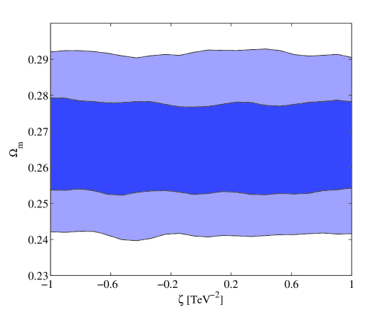
Figure 1: (Color Online) Contour plots of $\zeta$ vs $\Omega_{m}$ for a canonical field, that is for $\varepsilon=+1$, in the case of the exponential potential (4.1), under SNIa, BAO and CMB observational data. The white region is excluded at the 2$\sigma$ level, the light blue (light) region is excluded at the 1$\sigma$ level, and the blue (darkest) region is not excluded at either confidence level.

Concerning the units of $\zeta$ we use TeV^-2 in order to be closer to the particle physics origin of $\zeta$ [53], having in mind that in units where $8\pi G=1$ we obtain $1$TeV${}^{-2}\sim 5\times 10^{30}$. Similarly, in Fig. 2 we present the likelihood contours for the parameter $\zeta$ for a canonical field in the case of the power-law potential (4.2).

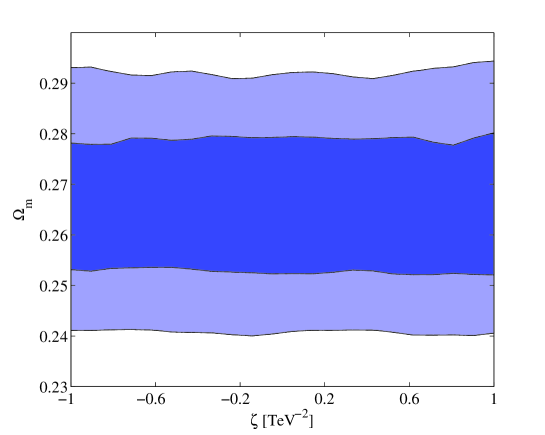
Figure 2: (Color Online) Contour plots of $\zeta$ vs $\Omega_{m}$, for a canonical field, that is for $\varepsilon=+1$, in the case of the power-law potential (4.2) for $n=2$, under SNIa, BAO and CMB observational data. The white region is excluded at the 2$\sigma$ level, the light blue (light) region is excluded at the 1$\sigma$ level, and the blue (darkest) region is not excluded at either confidence level.

As we observe from both figures, it seems that $\zeta$ remains quite unconstrained by the data. This is actually expected by observing the form of Friedmann equations (2.5) and (2.6), that is in order to have a significant effect we would approximately require $\zeta H^{2}\sim{\mathcal{O}}(1)$, which implies a huge value for $\zeta$ at current times. However, even such huge values would not have a significant effect since in the equations $\zeta$ always appears multiplied by $\phi^{\prime}$ or $\phi^{\prime 2}$, which are always very small, and thus $\zeta$-effects are negligible. In particular, in order to obtain a non-negligible effect of $\zeta$ on the Hubble parameter $\mathcal{H}$ (expressed in conformal time for convenience), we need to have $\zeta\phi^{\prime 2}/a^{2}\sim{\mathcal{O}}(1)$. However, this condition is never fulfilled since increasing $\zeta$ leads to a decrease in $\phi^{\prime}$, independently of the potential, as can be seen by the first term on the right hand side of the relation

$$\frac{d(a^{2}\phi^{\prime})}{d\ln a}=\left(\varepsilon+\frac{3\zeta{\cal H}^{2}}{a^{2}}+\frac{12\zeta^{2}{\cal H}^{2}\phi^{\prime 2}}{2a^{4}-a^{2}\zeta{\phi^{\prime 2}}}\right)^{-1}$$

$$\Big{\{}3\zeta{\phi^{\prime}}\left\{3{\cal H}^{2}+(2a^{2}-\zeta{\phi^{\prime 2}})^{-1}\left[{\varepsilon a^{2}\phi^{\prime 2}}+12\zeta{\cal H}^{2}\phi^{\prime 2}\right.\right.$$

$$\left.\left.\ \ \ -2a^{4}V(\phi)+2a^{4}(p_{dm}+p_{b}+p_{r})\right]\right\}-\frac{a^{4}V_{\phi}}{{\cal H}}\Big{\}},$$ (4.3)

which arises from (A.2)-(A.4).

In summary, when the scenario of non-minimal derivative coupling is quantitatively applied to late-time cosmology then the non-minimal derivative coupling term has a negligible effect on the background evolution, and thus the coupling parameter $\zeta$ remains quite unconstrained. We stress here that this result holds for the $\zeta$-term itself and not on the scenario as a whole. In other words the scenario of non-minimal derivative coupling can perfectly describe late-time acceleration, but the acceleration is driven by the usual potential term and not by the $\zeta$-term, that is the scenario practically coincides with standard quintessence (that is why in the above we did not present the usual contour plots of the various density parameters, since they practically coincide with those of standard quintessence [111]).

However, we mention that the present scenario can indeed have significant effects in early-time cosmology and in particular during inflation [45, 46, 47, 48, 49, 50, 51, 52, 53, 55]. The difference between the late-time and early-time application lies in the value of the Hubble parameter, which is huge during inflation, and thus along with the slow-roll approximation it allows the non-minimal derivative coupling to play a role even if it is quite small (since the “correction” term $9\zeta H^{2}$ will be indeed large).

5 Conclusions

In this work we performed a combined perturbation and observational investigation of the scenario of non-minimal derivative coupling between a scalar field and curvature. Both analyses are necessary in order to start applying the scenario as a realistic candidate for the description of the universe.

Concerning the perturbation examination, we extracted the necessary condition that ensures the absence of instabilities. As it is usual in higher-derivative models, a stable evolution is not guaranteed, that is a consistent cosmological application on the whole universe evolution would require a tuning on both the parameters and the initial conditions. However, we mention that, as expected, the stability improves significantly as the non-minimal derivative coupling parameter decreases (with its quintessence limit being always stable).

Concerning the observational constraining, our analyses shows that the non-minimal derivative coupling term cannot drive late-time acceleration. Note however that this result holds for this term itself and not for the scenario as a total, which can perfectly describe late-time acceleration, with the acceleration driven by the usual potential term and not by the $\zeta$-term, that is the scenario practically coincides with standard quintessence. On the contrary, during early-time evolution, the large Hubble-parameter value along with the slow-roll conditions allow even a small non-minimal derivative coupling term to drive inflation alone.

From these results we deduce that the non-minimal derivative coupling can drive inflation at early times, with the evolution being safe from instabilities since the required $\zeta$ is not large [53, 54]. On the other hand, at late times the usual potential term becomes the driving force of the universe acceleration, while the $\zeta$-terms has a negligible role, and the corresponding evolution remains instability-free since $\zeta$ still has the small value that was adequate for inflation [89, 90]. The combination of these evolutions makes the scenario of non-minimal derivative coupling a good candidate for the description of nature, since it can provide a unified picture of inflation and late-time acceleration. In such a case a detailed investigation of the perturbation evolution, and in particular of the growth of structure, would be necessary for the acceptance, constraining or exclusion of the scenario. Since such an analysis lies beyond the present work it is left for a future project.

Appendix A Equations in conformal time

For the purpose of this work, that is confronting the scenario with observations, it proves more convenient to write the cosmological equations using the conformal time $\eta$, which is related to the cosmic time $t$ through $dt=ad\eta$. Thus, using primes to denote differentiation with respect to $\eta$ and defining the conformal Hubble parameter as

$${\cal{H}}(\eta)=\frac{a^{\prime}(\eta)}{a(\eta)}=a(t)H(a(t)),$$ (A.1)

the two Friedmann equations become:

$$\frac{{\cal{H}}^{2}}{a^{2}}=\frac{8\pi G}{3}\left[\frac{\phi^{\prime 2}}{2a^{2}}\left(\varepsilon+9\zeta\frac{{\cal{H}}^{2}}{a^{2}}\right)+V(\phi)+\rho_{m}+\rho_{r}\right]\ \ \ \ \,\$$ (A.2)

$$2\frac{{\cal{H}}^{\prime}}{a^{2}}+\frac{{\cal{H}}^{2}}{a^{2}}=-8\pi G\left\{\frac{\phi^{\prime 2}}{2a^{2}}\left\{\varepsilon-\zeta\left[2\frac{{\cal{H}}^{\prime}}{a^{2}}+\frac{{\cal{H}}^{2}}{a^{2}}\right.\right.\right.$$

$$\left.\left.\left.\ \ \ \,\ \ +\frac{4{\cal{H}}}{a\phi^{\prime}}\left(\frac{\phi^{\prime\prime}}{a}-\frac{\phi^{\prime}{\cal{H}}}{a}\right)\right]\right\}-V(\phi)+p_{m}+p_{r}\right\},$$ (A.3)

while the field equation (2.7) writes as

$$\varepsilon\left(\frac{\phi^{\prime\prime}}{a^{2}}-\frac{\phi^{\prime}a^{\prime}}{a^{3}}+\frac{3{\cal{H}}\phi^{\prime}}{a^{2}}\right)+3\zeta\left(\frac{{\cal{H}}^{2}\phi^{\prime\prime}}{a^{4}}+\frac{2{\cal{H}}{\cal{H}}^{\prime}\phi^{\prime}}{a^{4}}\right)+V_{\phi}=0.$$ (A.4)

Finally, the energy density and pressure (2.8),(2.9) respectively write as

$$\rho_{DE}\equiv\rho_{\phi}=\frac{\phi^{\prime 2}}{2a^{2}}\left(\varepsilon+9\zeta\frac{{\cal{H}}^{2}}{a^{2}}\right)+V(\phi)\ \ \ \ \ \ \ \ \ \$$ (A.5)

$$p_{DE}\equiv p_{\phi}=\frac{\phi^{\prime 2}}{2a^{2}}\left\{\varepsilon-\zeta\left[2\frac{{\cal{H}}^{\prime}}{a^{2}}+\frac{{\cal{H}}^{2}}{a^{2}}+\frac{4{\cal{H}}}{a\phi^{\prime}}\left(\frac{\phi^{\prime\prime}}{a}-\frac{\phi^{\prime}{\cal{H}}}{a}\right)\right]\right\}-V(\phi).$$ (A.6)

One can verify that the scalar field equation A.4 can be written as

$$\rho^{\prime}_{DE}+3{\cal{H}}(\rho_{DE}+p_{DE})=0.$$ (A.7)

Appendix B Coefficients of perturbations equations

The various coefficients of the perturbation equation (3.15) are functions of $a,H,\dot{H},\phi,\dot{\phi},\ddot{\phi}$ and write as:

$$P_{1} = 8\pi G\left(-V-\rho_{m}+\frac{9}{2}\xi H^{2}\dot{\phi}^{2}\right)$$

$$P_{2} = 3H-\frac{9}{2}8\pi G\xi H\dot{\phi}^{2}$$

$$P_{3} = \frac{1}{a^{2}}\left(\frac{8\pi G\xi\dot{\phi}^{2}}{2}-1\right)$$

$$P_{4} = -8\pi GV^{\prime}$$

$$P_{5} = -8\pi G\dot{\phi}\left(1+9\xi H^{2}\right)$$

$$P_{6} = \frac{16\pi G\xi H\dot{\phi}}{a^{2}}$$

$$P_{7} = -8\pi G,$$

$$Q_{1} = \frac{1}{2}8\pi G\dot{\phi}^{2}+\left(3H^{2}+2\dot{H}\right)\left(1-\xi 8\pi G\dot{\phi}^{2}\right)-32\pi G\xi H\dot{\phi}\ddot{\phi}$$

$$Q_{2} = H\left(1-\frac{3}{2}\xi 8\pi G\dot{\phi}^{2}\right)$$

$$Q_{3} = \frac{2-8\pi G\xi\dot{\phi}^{2}}{6a^{2}}$$

$$Q_{4} = 8\pi GV-\frac{1}{2}8\pi G\dot{\phi}^{2}+16\pi G\xi H\dot{\phi}\ddot{\phi}+\left(\dot{H}+\frac{3}{2}H^{2}\right)\left(-2+8\pi G\xi\dot{\phi}^{2}\right)$$

$$Q_{5} = \frac{3}{2}H\left(-2+8\pi G\xi\dot{\phi}^{2}\right)+8\pi G\xi\dot{\phi}\ddot{\phi}$$

$$Q_{6} = -1+\frac{1}{2}8\pi G\xi\dot{\phi}^{2}$$

$$Q_{7} = \frac{2+8\pi G\xi\dot{\phi}^{2}}{6a^{2}}$$

$$Q_{8} = 8\pi GV^{\prime}$$

$$Q_{9} = 8\pi G\left[\left(-1+3\xi H^{2}+2\xi\dot{H}\right)\dot{\phi}+2\xi H\ddot{\phi}\right]$$

$$Q_{10} = 16\pi G\xi H\dot{\phi}$$

$$Q_{11} = -\frac{16\pi G\xi}{3a^{2}}\left(\ddot{\phi}+H\dot{\phi}\right),$$

$$R_{1} = H-\frac{3}{2}8\pi G\xi H\dot{\phi}^{2}$$

$$R_{2} = -1+\frac{1}{2}8\pi G\xi\dot{\phi}^{2}$$

$$R_{3} = -8\pi G\dot{\phi}\left(1+3\xi H^{2}\right)$$

$$R_{4} = 16\pi G\xi H\dot{\phi},$$

$$S_{1} = \frac{-2+8\pi G\xi\dot{\phi}^{2}}{4a^{2}}$$

$$S_{2} = \frac{-2-8\pi G\xi\dot{\phi}^{2}}{4a^{2}}$$

$$S_{3} = \frac{8\pi G\xi}{a^{2}}\left(\ddot{\phi}+H\dot{\phi}\right),$$

$$T_{1} = -V^{\prime}-\left(27\xi H^{3}-6H+18\xi H\dot{H}\right)\dot{\phi}-\left(2+9\xi H^{2}\right)\ddot{\phi}$$

$$T_{2} = -\frac{1}{2}\left(1+9\xi H^{2}\right)\dot{\phi}$$

$$T_{3} = \frac{-\xi H\dot{\phi}}{a^{2}}$$

$$T_{4} = \frac{3}{2}\left[\left(1+9\xi H^{2}+2\xi\dot{H}\right)\dot{\phi}+2\xi H\ddot{\phi}\right]$$

$$T_{5} = 3\xi H\dot{\phi}$$

$$T_{6} = -\frac{\xi}{a^{2}}\left(\ddot{\phi}+H\dot{\phi}\right)$$

$$T_{7} = V^{\prime\prime}$$

$$T_{8} = 18\xi H^{3}+6H+12\xi H\dot{H}+\frac{\ddot{\phi}\left(1+3\xi H^{2}\right)+V^{\prime}}{\dot{\phi}}$$

$$T_{9} = 1+3\xi H^{2}$$

$$T_{10} = -\frac{1+3\xi H^{2}+2\xi\dot{H}}{a^{2}},$$

$$U_{1} = -3H\rho_{m}-\dot{\rho}_{m}=0$$

$$U_{2} = 3\rho_{m}/2$$

$$U_{3} = 3H.$$

Additionally, the coefficients $C_{i}$ of the final perturbation equations (3.18)-(3.19) are functions of $t$ and $k$ and are given by

$$C_{1} = 0$$

$$C_{2} = -U_{2}$$

$$C_{3} = 0$$

$$C_{4} = 0$$

$$C_{5} = \left[\frac{Q_{10}S_{1}S_{2}T_{3}-Q_{10}S_{1}^{2}T_{6}+Q_{7}S_{1}^{2}T_{9}-Q_{3}S_{1}S_{2}T_{9}}{B}\right]k^{2}$$

$$+\frac{Q_{10}S_{2}T_{2}\dot{S}_{1}-Q_{10}S_{1}S_{2}T_{1}-Q_{4}S_{1}^{2}T_{9}+Q_{1}S_{1}S_{2}T_{9}}{B}$$

$$+\frac{Q_{2}S_{1}T_{9}\dot{S}_{2}-Q_{2}S_{2}T_{9}\dot{S}_{1}-Q_{10}S_{1}T_{2}\dot{S}_{2}}{B}$$

$$C_{6} = \frac{-Q_{10}S_{1}S_{2}T_{2}+Q_{10}S_{1}^{2}T_{4}-Q_{5}S_{1}^{2}T_{9}+Q_{2}S_{1}S_{2}T_{9}}{B}$$

$$C_{7} = \left[\frac{Q_{10}S_{1}S_{3}T_{3}-Q_{10}S_{1}^{2}T_{10}+Q_{11}S_{1}^{2}T_{9}-Q_{3}S_{1}S_{3}T_{9}}{B}\right]k^{2}$$

$$+\frac{Q_{10}S_{1}^{2}T_{7}-Q_{10}S_{1}S_{3}T_{1}-Q_{8}S_{1}^{2}T_{9}+Q_{1}S_{1}S_{3}T_{9}}{B}$$

$$+\frac{Q_{10}S_{3}T_{2}\dot{S}_{1}-Q_{2}S_{3}T_{9}\dot{S}_{1}-Q_{10}S_{1}T_{2}\dot{S}_{3}+Q_{2}S_{1}T_{9}\dot{S}_{3}}{B}$$

$$C_{8} = \frac{-Q_{10}S_{1}S_{3}T_{2}+Q_{10}S_{1}^{2}T_{8}-Q_{9}S_{1}^{2}T_{9}+Q_{2}S_{1}S_{3}T_{9}}{B}$$

$$C_{9} = \left[\frac{Q_{6}S_{1}S_{2}T_{3}+Q_{7}S_{1}^{2}T_{5}-Q_{3}S_{1}S_{2}T_{5}-Q_{6}S_{1}^{2}T_{6}}{B}\right]k^{2}$$

$$+\frac{Q_{6}S_{2}T_{2}\dot{S}_{1}-Q_{6}S_{1}S_{2}T_{1}-Q_{4}S_{1}^{2}T_{5}+Q_{1}S_{1}S_{2}T_{5}}{B}$$

$$+\frac{Q_{2}S_{1}T_{5}\dot{S}_{2}-Q_{2}S_{2}T_{5}\dot{S}_{1}-Q_{6}S_{1}T_{2}\dot{S}_{2}}{B}$$

$$C_{10} = \frac{-Q_{6}S_{2}T_{2}+Q_{6}S_{1}T_{4}-Q_{5}S_{1}T_{5}+Q_{2}S_{2}T_{5}}{B}$$

$$C_{11} = \left[\frac{-Q_{6}S_{1}^{2}T_{10}+Q_{6}S_{1}S_{3}T_{3}+Q_{11}S_{1}^{2}T_{5}-Q_{3}S_{1}S_{3}T_{5}}{B}\right]k^{2}$$

$$+\frac{Q_{6}S_{1}^{2}T_{7}-Q_{6}S_{1}S_{3}T_{1}-Q_{8}S_{1}^{2}T_{5}+Q_{1}S_{1}S_{3}T_{5}}{B}$$

$$+\frac{Q_{6}S_{3}T_{2}\dot{S}_{1}-Q_{2}S_{3}T_{5}\dot{S}_{1}-Q_{6}S_{1}T_{2}\dot{S}_{3}+Q_{2}S_{1}T_{5}\dot{S}_{3}}{B}$$

$$C_{12} = \frac{-Q_{6}S_{3}T_{2}-Q_{9}S_{1}T_{5}+Q_{2}S_{3}T_{5}+Q_{6}S_{1}T_{8}}{B},$$

with $B=S_{1}\left(Q_{10}T_{5}-Q_{6}T_{9}\right)$.

Appendix C Observational data and constraints

In the following we review briefly the main sources of observational constraints used in the present analysis, namely Type Ia Supernovae, Baryon Acoustic Oscillations (BAO) and Cosmic Microwave Background (CMB).

a. Type Ia Supernovae constraints

In order to take into account supernova constraints we use the Union 2.1 compilation of SnIa data [112]. This is a heterogeneous data-set, with data from the Supernova Legacy Survey, the Essence survey and the Hubble-Space-Telescope observed distant supernovae.

The corresponding $\chi^{2}$ is given by

$$\chi^{2}_{SN}=\frac{{\sum\limits_{i=1}^{N}{\left[{\mu_{\text{obs}}\left({z_{i}}\right)-\mu_{\rm th}\left({z_{i}}\right)}\right]}^{2}}}{{\sigma^{2}_{\mu,i}}},$$ (C.1)

where $N=580$ is the number of SNIa data points. $\mu_{\rm obs}$ is the observed distance modulus, defined as the difference between the supernova apparent and absolute magnitude. Additionally, $\sigma_{\mu,i}$ are the errors in the observed distance moduli, arising from a variety of sources, and assumed to be uncorrelated and Gaussian. The theoretical distance modulus $\mu_{\rm th}$ depends on the model parameters $a_{i}$ through the dimensionless luminosity distance $D_{L}(z;a_{i})$ given by

$$D_{L}\left(z;a_{i}\right)\equiv\left(1+z\right)\int^{z}_{0}dz^{\prime}\frac{H_{0}}{H\left(z^{\prime};a_{i}\right)},$$ (C.2)

as:

$$\mu_{\rm th}\left(z\right)=42.38-5\log_{10}h+5\log_{10}\left[D_{L}\left(z;a_{i}\right)\right].$$ (C.3)

The marginalization over the present Hubble parameter value is performed following the procedures described in [113], leading to the construction of $\chi^{2}$ likelihood contours for the involved model parameters.

b. Baryon Acoustic Oscillation constraints

The measured quantity in this class of observations is the ratio $d_{z}=r_{s}\left(z_{d}\right)/D_{V}\left(z\right)$, with $D_{V}\left(z\right)$ the “volume distance”, defined through the angular diameter distance $D_{A}\equiv r\left(z\right)/\left(1+z\right)$ as

$$D_{v}\left(z\right)\equiv\left[\frac{\left(1+z\right)^{2}D_{A}^{2}(z)z}{H(z)}\right]^{1/3},$$ (C.4)

and $z_{d}$ the baryon drag-epoch redshift calculated with the fitting formula [114]

$$z_{d}=\frac{1291\left(\Omega_{dm0}h^{2}\right)^{0.251}}{1+\left(\Omega_{dm0}h^{2}\right)^{0.828}}\left[1+b_{1}\left(\Omega_{b0}h^{2}\right)^{b_{2}}\right],$$ (C.5)

where $b_{1}$ and $b_{2}$ write as

$$b_{1} = 0.313\left(\Omega_{dm0}h^{2}\right)^{-0.419}\left[1+0.607\left(\Omega_{dm0}h^{2}\right)^{0.674}\right]$$

$$b2 = 0.238\left(\Omega_{dm0}h^{2}\right)^{0.223}.$$

In the present work we use the two $d_{z}$-measurements at redshifts $z=0.2$ and $z=0.35$ [115]. Thus, the $\chi^{2}$ contribution of the BAO measurements is calculated as

$$\chi^{2}_{BAO}=\mathbf{V}_{\rm BAO}^{\mathbf{T}}\mathbf{C}_{\rm inv}\mathbf{V}_{\rm BAO},$$ (C.6)

with $\mathbf{V}_{\rm BAO}\equiv\mathbf{P}-\mathbf{P}_{\rm data}$, where the vectors $\mathbf{P}\equiv\left(d_{0.2},d_{0.35}\right)$ and $\mathbf{P}_{\rm data}\equiv\left(0.1905,0.1097\right)$, are formed by the two measured BAO data points [115]. Lastly, the inverse covariance matrix is also given in [115].

c. CMB constraints

The incorporation of CMB data is performed following the techniques of [116]. We define the “CMB shift parameters” [117, 118] as

$$R\equiv\sqrt{\Omega_{dm0}}H_{0}r\left(z_{*}\right),\,\quad l_{a}\equiv\pi r\left(z_{*}\right)/r_{s}\left(z_{*}\right),$$ (C.7)

where the physical interpretation of $R$ is a scaled distance to recombination, and $l_{a}$ can be interpreted as the angular scale of the recombination sound horizon. Additionally, $r(z)$ is the comoving distance to redshift $z$ given by

$$r(z)\equiv\int_{0}^{z}\frac{1}{H\left(z\right)}dz,$$ (C.8)

while $r_{s}\left(z_{*}\right)$ is the comoving sound horizon at decoupling (corresponding to redshift $z_{*}$), which reads

$$r_{s}\left(z_{*}\right)=\int_{z_{*}}^{\infty}\frac{1}{H\left(z\right)\sqrt{3\left[1+R_{b}/\left(1+z\right)\right]}}dz.$$ (C.9)

$R_{b}$ is the ratio of the energy densities of photons to baryons, and its value is calculated to be $R_{b}=31500\Omega_{b0}h^{2}\left(T_{CMB}/2.7K\right)^{-4}$, (where $\Omega_{b0}$ is the present baryon density parameter) with $T_{CMB}=2.725$ [116]. The decoupling redshift $z_{*}\left(\Omega_{b0},\Omega_{dm0},h\right)$ can be estimated from the fitting formula [119]

$$z_{*}=1048\left[1+0.00124\left(\Omega_{b0}h^{2}\right)^{-0.738}\right]\left[1+g_{1}\left(\Omega_{dm0}h^{2}\right)^{g_{2}}\right],$$ (C.10)

where $g_{1}$ and $g_{2}$ read

$$g_{1} = \frac{0.0783\left(\Omega_{b0}h^{2}\right)^{-0.238}}{1+39.5\left(\Omega_{b0}h^{2}\right)^{0.763}}$$

$$g_{2} = \frac{0.560}{1+21.1\left(\Omega_{b0}h^{2}\right)^{1.81}}.$$

Then, the $\chi^{2}$ contribution of the CMB reads

$$\chi^{2}_{CMB}=\mathbf{V}_{\rm CMB}^{\mathbf{T}}\mathbf{C}_{\rm inv}\mathbf{V}_{\rm CMB},$$ (C.11)

with $\mathbf{V}_{\rm CMB}\equiv\mathbf{P}-\mathbf{P}_{\rm data}$, where $\mathbf{P}$ is the vector $\left(l_{a},R,z_{*}\right)$ and the vector $\mathbf{P}_{\rm data}$ is created from the WMAP $9$-year maximum likelihood values of these quantities [116]. Finally, the inverse covariance matrix $\mathbf{C}_{\rm inv}$ is also provided in [116].

References

- [1] A. G. Riess et al. [Supernova Search Team Collaboration], Observational evidence from supernovae for an accelerating universe and a cosmological constant, Astron. J. 116, 1009 (1998), [arXiv:astro-ph/9805201].
- [2] S. Perlmutter et al. [Supernova Cosmology Project Collaboration], Measurements of Omega and Lambda from 42 high redshift supernovae, Astrophys. J. 517, 565 (1999), [arXiv:astro-ph/9812133].
- [3] S. Capozziello and M. De Laurentis, Extended Theories of Gravity, Phys. Rept. 509, 167 (2011), [arXiv:1108.6266].
- [4] B. Ratra and P. J. E. Peebles, Cosmological Consequences of a Rolling Homogeneous Scalar Field, Phys. Rev. D 37, 3406 (1988).
- [5] C. Wetterich, Cosmology and the Fate of Dilatation Symmetry, Nucl. Phys. B 302, 668 (1988).
- [6] A. R. Liddle and R. J. Scherrer, A Classification of scalar field potentials with cosmological scaling solutions, Phys. Rev. D 59, 023509 (1999), [arXiv:astro-ph/9809272].
- [7] S. Basilakos and M. Plionis, Galaxy bias in quintessence cosmological models, Astrophys. J. 593, L61 (2003), [arXiv:astro-ph/0306105].
- [8] Z. -K. Guo, N. Ohta and Y. -Z. Zhang, Parametrizations of the dark energy density and scalar potentials, Mod. Phys. Lett. A 22, 883 (2007), [arXiv:astro-ph/0603109].
- [9] S. Dutta and R. J. Scherrer, Hilltop Quintessence, Phys. Rev. D 78, 123525 (2008), [arXiv:0809.4441].
- [10] S. Dutta, E. N. Saridakis and R. J. Scherrer, Dark energy from a quintessence (phantom) field rolling near potential minimum (maximum), Phys. Rev. D 79, 103005 (2009), [arXiv:0903.3412].
- [11] R. R. Caldwell, A Phantom menace?, Phys. Lett. B 545, 23 (2002), [arXiv:astro-ph/9908168].
- [12] R. R. Caldwell, M. Kamionkowski and N. N. Weinberg, Phantom energy and cosmic doomsday, Phys. Rev. Lett. 91, 071301 (2003), [arXiv:astro-ph/0302506].
- [13] S. ’i. Nojiri and S. D. Odintsov, Quantum de Sitter cosmology and phantom matter, Phys. Lett. B 562, 147 (2003), [arXiv:hep-th/0303117].
- [14] V. K. Onemli and R. P. Woodard, Quantum effects can render on cosmological scales, Phys. Rev. D 70, 107301 (2004), [arXiv:gr-qc/0406098].
- [15] E. N. Saridakis, Theoretical Limits on the Equation-of-State Parameter of Phantom Cosmology, Phys. Lett. B 676, 7 (2009), [arXiv:0811.1333].
- [16] S. Dutta and R. J. Scherrer, Dark Energy from a Phantom Field Near a Local Potential Minimum, Phys. Lett. B 676, 12 (2009), [arXiv:0902.1004].
- [17] B. Feng, X. L. Wang and X. M. Zhang, Dark Energy Constraints from the Cosmic Age and Supernova, Phys. Lett. B 607, 35 (2005), [arXiv:astro-ph/0404224].
- [18] Z. K. Guo, Y. S. Piao, X. M. Zhang and Y. Z. Zhang, Cosmological evolution of a quintom model of dark energy, Phys. Lett. B 608, 177 (2005), [arXiv:astro-ph/0410654].
- [19] W. Zhao, Quintom models with an equation of state crossing -1, Phys. Rev. D 73, 123509 (2006), [arXiv:astro-ph/0604460].
- [20] M. R. Setare and E. N. Saridakis, Coupled oscillators as models of quintom dark energy, Phys. Lett. B 668, 177 (2008), [arXiv:0802.2595].
- [21] M. R. Setare and E. N. Saridakis, Quintom model with O(N) symmetry, JCAP 0809, 026 (2008), [arXiv:0809.0114].
- [22] Y. F. Cai, E. N. Saridakis, M. R. Setare and J. Q. Xia, Quintom Cosmology: Theoretical implications and observations, Phys. Rept. 493, 1 (2010), [arXiv:0909.2776].
- [23] M. Khurshudyan and A. Khurshudyan, A model of a varying Ghost Dark energy, [arXiv:1307.7859].
- [24] E. J. Copeland, M. Sami and S. Tsujikawa, Dynamics of dark energy, Int. J. Mod. Phys. D 15, 1753 (2006), [arXiv:hep-th/0603057].
- [25] S. ’i. Nojiri, S. D. Odintsov, Introduction to modified gravity and gravitational alternative for dark energy, [arXiv:hep-th/0601213].
- [26] J. E. Lidsey, A. R. Liddle, E. W. Kolb, E. J. Copeland, T. Barreiro and M. Abney, Reconstructing the inflation potential : An overview, Rev. Mod. Phys. 69, 373 (1997), [arXiv:astro-ph/9508078].
- [27] V. Sahni and A. Starobinsky, Reconstructing Dark Energy, Int. J. Mod. Phys. D 15, 2105 (2006), [arXiv:astro-ph/0610026].
- [28] V. Sahni and S. Habib, Does inflationary particle production suggest Omega(m) less than 1?, Phys. Rev. Lett. 81, 1766 (1998), [arXiv:hep-ph/9808204].
- [29] J. -P. Uzan, Cosmological scaling solutions of nonminimally coupled scalar fields, Phys. Rev. D 59, 123510 (1999), [arXiv:gr-qc/9903004].
- [30] N. Bartolo and M. Pietroni, Scalar tensor gravity and quintessence, Phys. Rev. D 61, 023518 (2000), [arXiv:hep-ph/9908521].
- [31] O. Bertolami and P. J. Martins, Nonminimal coupling and quintessence, Phys. Rev. D 61, 064007 (2000), [arXiv:gr-qc/9910056].
- [32] B. Boisseau, G. Esposito-Farese, D. Polarski and A. A. Starobinsky, Reconstruction of a scalar tensor theory of gravity in an accelerating universe, Phys. Rev. Lett. 85, 2236 (2000), [arXiv:gr-qc/0001066]
- [33] V. Faraoni, Inflation and quintessence with nonminimal coupling, Phys. Rev. D 62, 023504 (2000), [arXiv:gr-qc/0002091].
- [34] R. de Ritis, A. A. Marino, C. Rubano and P. Scudellaro, Tracker fields from nonminimally coupled theory, Phys. Rev. D 62, 043506 (2000), [arXiv:hep-th/9907198].
- [35] S. Sen and A. A. Sen, Late time acceleration in Brans-Dicke cosmology, Phys. Rev. D 63, 124006 (2001), [arXiv:gr-qc/0010092].
- [36] K. Farakos and P. Pasipoularides, Gauss-Bonnet gravity, brane world models, and non-minimal coupling, Phys. Rev. D 75, 024018 (2007), [arXiv:hep-th/0610010].
- [37] S. ’i. Nojiri, S. D. Odintsov and M. Sami, Dark energy cosmology from higher-order, string-inspired gravity and its reconstruction, Phys. Rev. D 74, 046004 (2006), [arXiv:hep-th/0605039].
- [38] R. Gannouji, D. Polarski, A. Ranquet and A. A. Starobinsky, Scalar-Tensor Models of Normal and Phantom Dark Energy, JCAP 0609, 016 (2006), [arXiv:astro-ph/0606287].
- [39] K. Farakos, G. Koutsoumbas and P. Pasipoularides, Graviton localization and Newton’s law for brane models with a non-minimally coupled bulk scalar field, Phys. Rev. D 76, 064025 (2007), [arXiv:0705.2364].
- [40] M. Szydlowski, O. Hrycyna and A. Kurek, Coupling constant constraints in a nonminimally coupled phantom cosmology, Phys. Rev. D 77, 027302 (2008), [arXiv:0710.0366].
- [41] M. R. Setare and E. N. Saridakis, Non-minimally coupled canonical, phantom and quintom models of holographic dark energy, Phys. Lett. B 671, 331 (2009), [arXiv:0810.0645].
- [42] M. R. Setare and E. N. Saridakis, Braneworld models with a non-minimally coupled phantom bulk field: A Simple way to obtain the -1-crossing at late times, JCAP 0903, 002 (2009), [arXiv:0811.4253].
- [43] G. Gupta, E. N. Saridakis and A. A. Sen, Non-minimal quintessence and phantom with nearly flat potentials, Phys. Rev. D 79, 123013 (2009), [arXiv:0905.2348].
- [44] L. Amendola, Cosmology with nonminimal derivative couplings, Phys. Lett. B 301, 175 (1993), [arXiv:gr-qc/9302010].
- [45] S. Capozziello and G. Lambiase, Nonminimal derivative coupling and the recovering of cosmological constant, Gen. Rel. Grav. 31, 1005 (1999), [arXiv:gr-qc/9901051].
- [46] S. Capozziello, G. Lambiase and H. J. Schmidt, Nonminimal derivative couplings and inflation in generalized theories of gravity, Annalen Phys. 9, 39 (2000), [arXiv:gr-qc/9906051].
- [47] S. F. Daniel and R. R. Caldwell, Consequences of a cosmic scalar with kinetic coupling to curvature, Class. Quant. Grav. 24, 5573 (2007), [arXiv:0709.0009].
- [48] A. B. Balakin, H. Dehnen and A. E. Zayats, Effective metrics in the non-minimal Einstein-Yang-Mills-Higgs theory, Annals Phys. 323, 2183 (2008), [arXiv:0804.2196].
- [49] L. N. Granda, Inflation driven by scalar field with non-minimal kinetic coupling with Higgs and quadratic potentials, JCAP 1104, 016 (2011), [arXiv:1104.2253].
- [50] H. M. Sadjadi and P. Goodarzi, Reheating in nonminimal derivative coupling model, JCAP 1302, 038 (2013), [arXiv:1203.1580].
- [51] K. Feng, T. Qiu and Y. -S. Piao, Curvaton with nonminimal derivative coupling to gravity, [arXiv:1307.7864].
- [52] H. M. Sadjadi and P. Goodarzi, Oscillatory inflation in non-minimal derivative coupling mode, [arXiv:1309.2932].
- [53] C. Germani and A. Kehagias, New Model of Inflation with Non-minimal Derivative Coupling of Standard Model Higgs Boson to Gravity, Phys. Rev. Lett. 105, 011302 (2010), [arXiv:1003.2635].
- [54] C. Germani and A. Kehagias, Cosmological Perturbations in the New Higgs Inflation, JCAP 1005, 019 (2010), [arXiv:1003.4285].
- [55] S. Tsujikawa, Observational tests of inflation with a field derivative coupling to gravity, Phys. Rev. D 85, 083518 (2012), [arXiv:1201.5926].
- [56] S. V. Sushkov, Exact cosmological solutions with nonminimal derivative coupling, Phys. Rev. D 80, 103505 (2009), [arXiv:0910.0980].
- [57] E. N. Saridakis and S. V. Sushkov, Quintessence and phantom cosmology with non-minimal derivative coupling, Phys. Rev. D 81, 083510 (2010), [arXiv:1002.3478].
- [58] C. Gao, When scalar field is kinetically coupled to the Einstein tensor, JCAP 1006, 023 (2010), [arXiv:1002.4035].
- [59] L. N. Granda and W. Cardona, General Non-minimal Kinetic coupling to gravity, JCAP 1007, 021 (2010), [arXiv:1005.2716].
- [60] S. Chen and J. Jing, Greybody factor for a scalar field coupling to Einstein’s tensor, Phys. Lett. B 691, 254 (2010), [arXiv:1005.5601].
- [61] S. Chen and J. Jing, Dynamical evolution of a scalar field coupling to Einstein’s tensor in the Reissner-Nordstróm black hole spacetime, Phys. Rev. D 82, 084006 (2010), [arXiv:1007.2019].
- [62] C. Deffayet, O. Pujolas, I. Sawicki and A. Vikman, Imperfect Dark Energy from Kinetic Gravity Braiding, JCAP 1010, 026 (2010), [arXiv:1008.0048].
- [63] K. Karwan, Dynamics of entropy perturbations in assisted dark energy with mixed kinetic terms, JCAP 1102, 007 (2011), [arXiv:1009.2179].
- [64] L. N. Granda, Non-minimal kinetic coupling and the phenomenology of dark energy, Class. Quant. Grav. 28, 025006 (2011), [arXiv:1009.3964].
- [65] H. M. Sadjadi, Super-acceleration in non-minimal derivative coupling model, Phys. Rev. D 83, 107301 (2011), [arXiv:1012.5719].
- [66] K. Van Acoleyen and J. Van Doorsselaere, Galileons from Lovelock actions, Phys. Rev. D 83, 084025 (2011), [arXiv:1102.0487].
- [67] V. K. Shchigolev and M. P. Rotova, Modelling Tachyon Cosmology with Non-Minimal Derivative Coupling to Gravity, Grav. Cosmol. 18, 88 (2012), [arXiv:1105.4536].
- [68] A. Banijamali and B. Fazlpour, Crossing of with Tachyon and Non-minimal Derivative Coupling, Phys. Lett. B 703, 366 (2011), [arXiv:1105.4967].
- [69] C. Charmousis, E. J. Copeland, A. Padilla and P. M. Saffin, General second order scalar-tensor theory, self tuning, and the Fab Four, Phys. Rev. Lett. 108, 051101 (2012), [arXiv:1106.2000].
- [70] L. N. Granda, E. Torrente-Lujan and J. J. Fernandez-Melgarejo, Non-minimal kinetic coupling and Chaplygin gas cosmology, Eur. Phys. J. C 71, 1704 (2011), [arXiv:1106.5482].
- [71] C. de Rham and L. Heisenberg, Cosmology of the Galileon from Massive Gravity, Phys. Rev. D 84, 043503 (2011), [arXiv:1106.3312].
- [72] L. N. Granda, Dark energy from scalar field with Gauss Bonnet and non-minimal kinetic coupling, Mod. Phys. Lett. A 27, 1250018 (2012), [arXiv:1108.6236].
- [73] T. Kolyvaris, G. Koutsoumbas, E. Papantonopoulos and G. Siopsis, Scalar Hair from a Derivative Coupling of a Scalar Field to the Einstein Tensor, Class. Quant. Grav. 29, 205011 (2012), [arXiv:1111.0263].
- [74] S. V. Sushkov and R. Korolev, Scalar wormholes with nonminimal derivative coupling, Class. Quant. Grav. 29, 085008 (2012), [arXiv:1111.3415].
- [75] A. Banijamali and B. Fazlpour, Phantom Behavior Bounce with Tachyon and Non-minimal Derivative Coupling, JCAP 1201, 039 (2012), [arXiv:1201.1627].
- [76] F. Farakos, C. Germani, A. Kehagias and E. N. Saridakis, A New Class of Four-Dimensional N=1 Supergravity with Non-minimal Derivative Couplings, JHEP 1205, 050 (2012), [arXiv:1202.3780].
- [77] J. -P. Bruneton, M. Rinaldi, A. Kanfon, A. Hees, S. Schlogel and A. Fuzfa, Fab Four: When John and George play gravitation and cosmology, Adv. Astron. 2012, 430694 (2012), [arXiv:1203.4446].
- [78] J. -A. Gu, C. -C. Lee and C. -Q. Geng, Teleparallel Dark Energy with Purely Non-minimal Coupling to Gravity, Phys. Lett. B 718, 722 (2013), [arXiv:1204.4048].
- [79] K. Bamba, S. Capozziello, S. ’i. Nojiri and S. D. Odintsov, Dark energy cosmology: the equivalent description via different theoretical models and cosmography tests, Astrophys. Space Sci. 342, 155 (2012), [arXiv:1205.3421].
- [80] A. Banijamali, B. Fazlpour and B. Fazlpour, Phantom Divide Crossing with General Non-minimal Kinetic Coupling, [arXiv:1206.3299].
- [81] A. Banijamali, J. Sadeghi and H. Vaez, Tachyon cosmology with nonminimal derivative coupling, Can. J. Phys. 90, 999 (2012).
- [82] M. Sami, M. Shahalam, M. Skugoreva, A. Toporensky, M. Shahalam, M. Skugoreva and A. Toporensky, Cosmological dynamics of non-minimally coupled scalar field system and its late time cosmic relevance, Phys. Rev. D 86, 103532 (2012), [arXiv:1207.6691].
- [83] J. Li and Y. Zhong, Dynamical evolution of a scalar field coupling to Einstein’s tensor in charged braneworld black holes, Int. J. Theor. Phys. 51, 2585 (2012).
- [84] L. N. Granda and E. Loaiza, Exact solutions in a scalar-tensor model of dark energy, JCAP 1209, 011 (2012), [arXiv:1209.1137].
- [85] H. M. Sadjadi and P. Goodarzi, Reheating temperature in non-minimal derivative coupling model, JCAP 1307, 039 (2013), [arXiv:1302.1177].
- [86] G. Koutsoumbas, K. Ntrekis and E. Papantonopoulos, Gravitational Particle Production in Gravity Theories with Non-minimal Derivative Couplings, JCAP 1308, 027 (2013), [arXiv:1305.5741].
- [87] Y. Zhou, Non-minimal coupling scalar field quasinormal modes of Schwarzschild-de Sitter black hole with a global monopole, Int. J. Theor. Phys. 52, 1431 (2013).
- [88] T. Kolyvaris, G. Koutsoumbas, E. Papantonopoulos and G. Siopsis, Phase Transition to a Hairy Black Hole in Asymptotically Flat Spacetime, [arXiv:1308.5280].
- [89] S. Sushkov, Realistic cosmological scenario with non-minimal kinetic coupling, Phys. Rev. D 85, 123520 (2012), [arXiv:1204.6372].
- [90] M. A. Skugoreva, S. V. Sushkov and A. V. Toporensky, Cosmology with nonminimal kinetic coupling and a power-law potential, [arXiv:1306.5090].
- [91] J. M. Cline, S. Jeon and G. D. Moore, The phantom menaced: Constraints on low-energy effective ghosts, Phys. Rev. D 70, 043543 (2004), [arXiv:hep-ph/0311312].
- [92] G. Leon and E. N. Saridakis, Dynamical analysis of generalized Galileon cosmology, JCAP 1303, 025 (2013), [arXiv:1211.3088].
- [93] A. De Felice and S. Tsujikawa, Conditions for the cosmological viability of the most general scalar-tensor theories and their applications to extended Galileon dark energy models, JCAP 1202, 007 (2012), [arXiv:1110.3878].
- [94] G. L. Goon, K. Hinterbichler and M. Trodden, Stability and superluminality of spherical DBI galileon solutions, Phys. Rev. D 83, 085015 (2011), [arXiv:1008.4580].
- [95] C. Burrage, C. de Rham, L. Heisenberg and A. J. Tolley, Chronology Protection in Galileon Models and Massive Gravity, JCAP 1207, 004 (2012), [arXiv:1111.5549].
- [96] C. Germani, On the Covariant Galileon and a consistent self-accelerating Universe, Phys. Rev. D 86, 104032 (2012), [arXiv:1207.6414].
- [97] P. de Fromont, C. de Rham, L. Heisenberg and A. Matas, Superluminality in the Bi- and Multi- Galileon, JHEP 1307, 067 (2013), [arXiv:1303.0274].
- [98] R. J. Scherrer and A. A. Sen, Thawing quintessence with a nearly flat potential, Phys. Rev. D 77, 083515 (2008), [arXiv:0712.3450].
- [99] R. J. Scherrer and A. A. Sen, Phantom Dark Energy Models with a Nearly Flat Potential, Phys. Rev. D 78, 067303 (2008), [arXiv:0808.1880].
- [100] M. R. Setare and E. N. Saridakis, Quintom dark energy models with nearly flat potentials, Phys. Rev. D 79, 043005 (2009), [arXiv:0810.4775].
- [101] E. J. Copeland, A. RLiddle and D. Wands, Exponential potentials and cosmological scaling solutions, Phys. Rev. D 57, 4686 (1998), [arXiv:gr-qc/9711068].
- [102] P. G. Ferreira and M. Joyce, Structure formation with a selftuning scalar field, Phys. Rev. Lett. 79, 4740 (1997), [arXiv:astro-ph/9707286].
- [103] X. -m. Chen, Y. -g. Gong and E. N. Saridakis, Phase-space analysis of interacting phantom cosmology, JCAP 0904, 001 (2009), [arXiv:0812.1117].
- [104] G. Leon and E. N. Saridakis, Phase-space analysis of Horava-Lifshitz cosmology, JCAP 0911, 006 (2009), [arXiv:0909.3571].
- [105] A. de la Macorra and C. Stephan-Otto, Quintessence restrictions on negative power and condensate potentials, Phys. Rev. D 65, 083520 (2002), [arXiv:astro-ph/0110460].
- [106] J. P. Kneller and L. E. Strigari, Inverse power law quintessence with non-tracking initial conditions, Phys. Rev. D 68, 083517 (2003), [arXiv:astro-ph/0302167].
- [107] L. R. W. Abramo and F. Finelli, Cosmological dynamics of the tachyon with an inverse power-law potential, Phys. Lett. B 575, 165 (2003), [arXiv:astro-ph/0307208].
- [108] X. Zhang, Coupled quintessence in a power-law case and the cosmic coincidence problem, Mod. Phys. Lett. A 20, 2575 (2005), [arXiv:astro-ph/0503072].
- [109] E. N. Saridakis, Phantom evolution in power-law potentials, Nucl. Phys. B 819, 116 (2009), [arXiv:0902.3978].
- [110] E. N. Saridakis, Quintom evolution in power-law potentials, Nucl. Phys. B 830, 374 (2010), [arXiv:0903.3840].
- [111] P. A. R. Ade et al. [Planck Collaboration], Planck 2013 results. XVI. Cosmological parameters, [arXiv:1303.5076].
- [112] N. Suzuki, D. Rubin, C. Lidman, G. Aldering, R. Amanullah, K. Barbary, L. F. Barrientos and J. Botyanszki et al., The Hubble Space Telescope Cluster Supernova Survey: V. Improving the Dark Energy Constraints Above z¿1 and Building an Early-Type-Hosted Supernova Sample, Astrophys. J. 746, 85 (2012), [arXiv:1105.3470].
- [113] R. Lazkoz, S. Nesseris and L. Perivolaropoulos, Comparison of Standard Ruler and Standard Candle constraints on Dark Energy Models, JCAP 0807, 012 (2008), [arXiv:0712.1232].
- [114] D. J. Eisenstein and W. Hu, Baryonic Features in the Matter Transfer Function, Astrophys. J. 496, 605 (1998), [arXiv:astro-ph/9709112].
- [115] W. J. Percival et al. [SDSS Collaboration], Baryon Acoustic Oscillations in the Sloan Digital Sky Survey Data Release 7 Galaxy Sample, Mon. Not. Roy. Astron. Soc. 401, 2148 (2010), [arXiv:0907.1660].
- [116] G. Hinshaw et al. [WMAP Collaboration], Nine-Year Wilkinson Microwave Anisotropy Probe (WMAP) Observations: Cosmological Parameter Results, [arXiv:1212.5226].
- [117] Y. Wang and P. Mukherjee, Robust Dark Energy Constraints from Supernovae, Galaxy Clustering, and Three-Year Wilkinson Microwave Anisotropy Probe Observations, Astrophys. J. 650, 1 (2006), [arXiv:astro-ph/0604051].
- [118] Y. Wang and P. Mukherjee, Observational Constraints on Dark Energy and Cosmic Curvature, Phys. Rev. D 76, 103533 (2007), [arXiv:astro-ph/0703780].
- [119] W. Hu and N. Sugiyama, Small scale cosmological perturbations: An Analytic approach, Astrophys. J. 471, 542 (1996), [arXiv:astro-ph/9510117].