Parity violation in proton-proton scattering
from chiral effective field theory

J. de Vries¹, Ulf-G. Meißner^1,2, E. Epelbaum³, N. Kaiser⁴

¹ Institute for Advanced Simulation, Institut für Kernphysik, and Jülich Center for Hadron Physics, Forschungszentrum Jülich, D-52425 Jülich, Germany

² Helmholtz-Institut für Strahlen- und Kernphysik and Bethe Center for Theoretical Physics, Universität Bonn, D-53115 Bonn, Germany

³ Institut für Theoretische Physik II, Ruhr-Universität Bochum, 44780 Bochum, Germany

⁴ Physik Department T39, Technische Universität München, D-85747 Garching, Germany

We present a calculation of the parity-violating longitudinal asymmetry in proton-proton scattering. The calculation is performed in the framework of chiral effective field theory which is applied systematically to both the parity-conserving and parity-violating interactions. The asymmetry is calculated up to next-to-leading order in the parity-odd nucleon-nucleon potential. At this order the asymmetry depends on two parity-violating low-energy constants: the weak pion-nucleon coupling constant $h_{\pi}$ and one four-nucleon contact coupling. By comparison with the existing data, we obtain a rather large range for $h_{\pi}=(1.1\pm 2)\cdot 10^{-6}$. This range is consistent with theoretical estimations and experimental limits, but more data are needed to pin down a better constrained value. We conclude that an additional measurement of the asymmetry around $125$ MeV lab energy would be beneficial to achieve this goal.

1 Introduction

The observation of parity ($P$) violation in the weak interaction is one of the pillars on which the Standard Model of particle physics was built. In the Standard Model parity violation is implemented by specifying different gauge-symmetry representations of the chiral fermions which has the consequence that only left-handed quarks and leptons participate in the (charged current) weak interaction. At the fundamental level, parity violation originates from the exchange of the charged (and neutral) weak gauge bosons. For low-energy (hadronic) processes, the heavy gauge bosons decouple from the theory leading to effective parity-violating four-fermion interactions. The effective interactions resulting from the exchange of charged gauge bosons induce, for example, the beta-decay of the muon and the neutron, while the exchange of neutral gauge bosons gives rise to various parity-violating four-quark operators.

Despite this theoretical foundation, the manifestation of the $P$-violating four-quark operators in hadronic and nuclear systems is not fully understood. The problem arises mainly from the nonperturbative nature of QCD at low energies. In order to circumvent this problem, the nucleon-nucleon ($N\!N$) interaction has been parametrized in the past through $P$-violating meson exchanges with adjustable strengths. Nevertheless, theoretically allowed ranges for the coupling constants could be estimated. This meson-exchange model is usually called the DDH-framework [1]. Given enough experimental input the unknown couplings can be determined and other processes can then be predicted. However, the extractions of the coupling constants from different experiments seem to be in disagreement, although a recent study [2] shows that a consistent picture does emerge if only results from few-body experiments are used in the analysis (for recent reviews, see Refs. [2, 3]).

In the last three decades tremendous progress has been made in understanding low-energy strong interactions by the application of effective field theories (EFTs). By writing down the most general Lagrangian for the relevant low-energy degrees of freedom that is consistent with the symmetries of the underlying theory, i.e QCD, one obtains an effective field theory, called chiral-perturbation theory ($\chi$PT), which is a low-energy equivalent of QCD (in the sense of fulfilling the same chiral Ward identities) (for a pedagogical review, see Ref. [4]). $\chi$PT has a major advantage that observables can be calculated perturbatively in the form of an expansion in $p/\Lambda_{\chi}$, where $p$ is the typical momentum of the process and $\Lambda_{\chi}\sim 1$ GeV the chiral symmetry breaking scale. In principle calculations can be performed up to any order although in practice the number of unknown low-energy constants (LECs) increases quickly which limits the predictive power. Another success of $\chi$PT is the explanation of the hierarchy and the form of multi-nucleon interactions with respect to $N\!N$ interactions. The strong $N\!N$ potential has been derived up to next-to-next-to-next-to-leading order (N³LO) and describes the $N\!N$ experimental database with a similar quality as the phenomenological “high-precision” potentials (for recent reviews, see Refs. [5, 6]).

The application of $\chi$PT has led to a derivation of the effective $P$-violating $N\!N$ potential. At leading order (LO) this potential consists of one-pion exchange involving as a parameter the weak pion-nucleon coupling constant $h_{\pi}$ [7]. At next-to-leading order (NLO) corrections appear due to $P$-violating two-pion exchange [8, 9] and five $P$-odd $N\!N$ contact interactions [8, 10, 11, 12] representing short-range dynamics (one for each $S\leftrightarrow P$ wave transition). These corrections are suppressed by two powers of $p/\Lambda_{\chi}$. Additional interactions involving external photons appear also at this order.

The effective $P$-violating $N\!N$ potential in combination with phenomenological $P$-conserving potentials have been applied in several so-called “hybrid” calculations. Full EFT calculations of $P$-violating effects in proton-proton ($pp$) scattering have only been performed within pionless EFT in which the pion is integrated out and both $P$-conserving and $P$-violating effects are described by $N\!N$ contact interactions [13]. Although this is a consistent framework, the absence of pions implies that the EFT is only applicable in the very low energy region $E\sim M_{\pi}^{2}/(2m_{N})\simeq 10.5$ MeV, while a pionfull treatment can be extended up to higher energies of a few hundred MeV. Additionally, by integrating out the pion, important information on the chiral-symmetry properties of the $P$-violating interactions gets lost. For a review, see Ref. [14].

In this paper we apply simultaneously $P$-even and $P$-odd chiral nuclear interactions in a systematic fashion. We focus on the calculation of the longitudinal analyzing power in $pp$ scattering for which several experimental data points exist. There are two special features that arise for $pp$ scattering. The first one is that the leading-order $N\!N$ potential which causes a ${}^{3}S_{1}\leftrightarrow{}^{3}P_{1}$ transition is forbidden for two identical protons. It becomes thus mandatory to consider the NLO $P$-odd potential which makes the analyzing power dependent on two independent LECs. Secondly, the presence of the Coulomb interaction complicates the calculation. We will discuss both issues in detail. Our main goal is to perform a careful extraction of the two LECs and compare these with theoretical estimates.

The present paper is organized as follows. In Sec. 2 we give the parity-violating $N\!N$ potential at NLO and summarize the present knowledge of the weak pion-nucleon coupling $h_{\pi}$. In Sec. 3 we discuss the Lippmann-Schwinger equation to solve the scattering problem in the presence of the Coulomb interaction and define the pertinent longitudinal analyzing power $A_{z}$ that measures the parity violation. Sec. 4 gives a detailed discussion of the extraction of the $P$-odd LECs from the data at low and intermediate energies. Sec. 5 contains a short summary and conclusions.

2 Parity-even and parity-odd nucleon-nucleon potentials

In this paper $P$-even and $P$-odd $N\!N$ potentials as obtained in chiral effective field theory [15, 16, 17, 18] are employed. In order to obtain a description of $N\!N$ scattering data with high precision, the chiral nucleon-nucleon potential has been extended up to N³LO in Refs. [19, 20]. Both approaches differ in the regularization scheme and the treatment of the cut-off appearing in the solution of the Lippmann-Schwinger equation. An advantage of the potential of Ref. [20] (which is also used here) is that the cut-off can be varied over a certain range which gives a handle on theoretical uncertainties. Obviously, the N³LO potential consists of many terms and we refer to Ref. [20] for further details. Let us continue with presenting the $P$-violating part of the $N\!N$ potential.

The $P$-odd $N\!N$ potential has been first derived in chiral perturbation theory in Refs. [7, 10, 11, 8]. At leading order it arises from the $P$-odd pion-nucleon interaction

$$\mathcal{L}_{/P}=\frac{h_{\pi}}{\sqrt{2}}\bar{N}(\vec{\pi}\times\vec{\tau})^{3}N,$$ (1)

with the coupling constant $h_{\pi}$. Here $N=(p\,n)^{t}$ denotes the nucleon isospin-doublet, $\vec{\pi}$ the pion isospin-triplet, and $\vec{\tau}$ the isospin Pauli matrices. In combination with the standard pseudovector parity-conserving pion-nucleon interaction, the leading-order $P$-odd one-pion-exchange (OPE) potential follows as

$$V_{\text{OPE}}=-\frac{g_{A}h_{\pi}}{2\sqrt{2}F_{\pi}}i(\vec{\tau}_{1}\times\vec{\tau}_{2})^{3}\frac{(\vec{\sigma}_{1}+\vec{\sigma}_{2})\cdot\vec{q}}{m_{\pi}^{2}+q^{2}},$$ (2)

with $\vec{q}=\vec{p}-\vec{p}^{\,\prime}$ ($q=|\vec{q}\,|$), where $\vec{p}$ and $\vec{p}^{\,\prime}$ are the relative momenta of the incoming and outgoing nucleon pair in the center-of-mass frame. $F_{\pi}=92.4$ MeV is the pion decay constant, $m_{\pi}=139.57$ MeV the charged pion mass, and $g_{A}=1.29$ the nucleon axial-vector coupling constant. By using this value of $g_{A}$ we have accounted for the Goldberger-Treiman discrepancy [20].

It is not hard to see that this OPE potential vanishes between states of equal total isospin and dominantly contributes to the ${}^{3}S_{1}\leftrightarrow{}^{3}P_{1}$ transition. The OPE potential therefore does not contribute to parity violation in $pp$ (or $nn$) scattering. The NLO corrections to the $P$-odd potential appear at relative order $(p/\Lambda_{\chi})^{2}$ and consist, among other contributions, of two-pion-exchange (TPE) diagrams [8, 9]. The TPE contributions come in the form of triangle, box, and crossed-box diagrams. The triangle diagrams lead to the same isospin operator $(\vec{\tau}_{1}\times\vec{\tau}_{2})^{3}$ as the OPE potential and do therefore not contribute to $pp$ scattering. Apart from a contribution with the same isospin-operator, the box and crossed-box diagrams sum up to

$$V_{\text{TPE}}=\frac{\sqrt{2}g^{3}_{A}h_{\pi}}{(4\pi F_{\pi})^{2}F_{\pi}}\left[i(\vec{\tau}_{1}+\vec{\tau}_{2})^{3}\,(\vec{\sigma}_{1}\times\vec{\sigma}_{2})\cdot\vec{q}\,\right]L(q,\Lambda_{S})\,,$$ (3)

in terms of the loop function

$$L(q,\Lambda_{S})=\frac{\omega}{2q}\ln\left(\frac{\Lambda_{S}^{2}\omega^{2}+q^{2}s^{2}+2\Lambda_{S}s\omega q}{4m_{\pi}^{2}(\Lambda_{S}^{2}+q^{2})}\right)\,,\qquad\omega=\sqrt{4m_{\pi}^{2}+q^{2}},\qquad s=\sqrt{\Lambda_{S}^{2}-4m_{\pi}^{2}}~{}.$$ (4)

Following Ref. [20] we have used the method of spectral regularization [21] to regularize the finite part of the pion-loop. The $P$-even $N\!N$ potential has been regularized in the same way with a spectral cut-off $\Lambda_{S}$.

The TPE diagrams are divergent and counter terms are necessary in order to absorb these divergences. Such counter terms naturally arise within chiral EFT and appear as $N\!N$ contact interactions at the same order as the TPE potential [8]. In principle, five independent contact interactions appear [12] but only one linear combination enters in $pp$ scattering. Writing this combination as $C$ gives the following contribution to the $P$-odd potential

$$V_{\text{CT}}=\frac{C}{2F_{\pi}\Lambda_{\chi}^{2}}\left[i(\vec{\tau}_{1}+\vec{\tau}_{2})^{3}(\vec{\sigma}_{1}\times\vec{\sigma}_{2})\cdot\vec{q}\,\right],$$ (5)

where $\Lambda_{\chi}=1$ GeV is the chiral symmetry breaking scale. The factor $(F_{\pi}\Lambda_{\chi}^{2})^{-1}$ is inserted in order to make $C$ dimensionless.

At the order of the TPE diagrams and counter terms, there appear corrections to the one-pion exchange $V_{\rm OPE}$ proportional to the quark mass. These corrections can be absorbed into coupling constant $h_{\pi}$. In the power-counting scheme of Ref. [20], relativistic and isospin-breaking corrections appear at higher order in the potential.

Summarizing, the relevant $P$-odd potential in the case of $pp$ scattering at NLO is simply given by $V_{\rm TPE}+V_{\rm CT}$ in Eqs. (3) and (5).

2.1 Estimates and limits of $h_{\pi}$

In an EFT, the LECs corresponding to the various effective interactions are a priori unknown and need to be determined by fitting them to experimental data. In the present case the microscopic theory is well-known, i.e. QCD supplemented with $P$-violating four-quark operators, which means that one can attempt to calculate the LECs directly. This is a highly non-trivial task due to the nonperturbativeness of QCD at low energies. Despite this difficulty, several approaches exist to tackle this problem.

Clearly the most simple one is the use of naive-dimensional analysis (NDA) [22, 23] which gives the following estimates

$$h_{\pi}\sim C\sim\mathcal{O}(G_{F}F_{\pi}\Lambda_{\chi})\sim 10^{-6},$$ (6)

in terms of the Fermi coupling constant $G_{F}$. This should be seen as an order-of-magnitude estimate, providing a rough scale for the size of parity violation in hadronic systems.

In the original DDH paper [1], the authors have attempted to estimate $h_{\pi}$, and several other LECs associated with heavier mesons, using $SU(6)$ symmetry arguments and the quark model. They have found a range of reasonable values for $h_{\pi}$:

$$0\leq h_{\pi}\leq 1.2\cdot 10^{-6},$$ (7)

and a “best” value of $h_{\pi}\simeq 4.6\cdot 10^{-7}$, consistent with the NDA estimate.

The authors of Ref. [24] have calculated several $P$-violating meson-nucleon vertices in a framework of a non-linear chiral Lagrangian where the nucleon emerges as a soliton. They have obtained significantly smaller values for $h_{\pi}\simeq 0.2\cdot 10^{-7}$. This approach simultaneously predicts the strong meson-nucleon coupling constants which were found to be in good agreement with phenomenological boson-exchange models. In Ref. [25], the calculation of $h_{\pi}$ has been sharpened based on a three-flavor Skyrme model calculation with the result $h_{\pi}\simeq 1\cdot 10^{-7}$, which lies in between the DDH best value and the results of Ref. [24].

Recently, the first lattice QCD calculation has been made for $h_{\pi}$ using a lattice size of $2.5\,\mathrm{fm}$ and a pion mass $M_{\pi}\simeq 389\,\mathrm{MeV}$, finding the result

$$h_{\pi}=\left(1.1\pm 0.5\,(\mathrm{stat})\pm 0.5\,(\mathrm{sys})\right)\cdot 10^{-7},$$ (8)

which is also rather small with respect to the DDH range [26]. It should be noted that this result does not contain contributions from disconnected diagrams nor was the result extrapolated to the physical pion mass.

The smaller estimates seem to be in better agreement with data. Experiments on $\gamma$-ray emission from ${}^{18}F$ set the rather strong upper limit [27, 28]

$$h_{\pi}<1.3\cdot 10^{-7}~{}.$$ (9)

Although calculations for nuclei bring in additional uncertainties, in this case these can to a certain extent be “cancelled out” by comparison with the analogous $\beta$-decay of ${}^{18}\mathrm{Ne}$ [29].

Historically, the calculation of the longitudinal asymmetry in $pp$ scattering has not been done in terms of $h_{\pi}$ because, as mentioned above, the OPE potential does not contribute. Within the modern EFT approach, this argument is no longer valid because $h_{\pi}$ contributes via the two-pion-exchange potential. So far, these contributions have been considered in a hybrid approach in Refs. [30, 31]. In this paper, we investigate within a full EFT approach which ranges of $h_{\pi}$ and $C$ are consistent with existing data and how these ranges relate to the above estimates and limits.

3 Aspects of the calculation

We apply the following form of the non-relativistic Lippmann-Schwinger (LS) equation in momentum space

$$T^{l^{\prime}l\,s^{\prime}s}_{j}(p^{\prime},p,E)=V^{l^{\prime}l\,s^{\prime}s}_{j}(p^{\prime},p)+\sum_{l^{\prime\prime}\,s^{\prime\prime}}\int_{0}^{\infty}dp^{\prime\prime}\,V^{l^{\prime}l^{\prime\prime}\,s^{\prime}s^{\prime\prime}}_{j}(p^{\prime},p^{\prime\prime})\left(\frac{p^{\prime\prime\,2}}{E-p^{\prime\prime\,2}/m_{p}+i\epsilon}\right)T^{l^{\prime\prime}l\,s^{\prime\prime}s}_{j}(p^{\prime\prime},p,E)~{},$$ (10)

where $E$ is the center-of-mass energy and $m_{p}=938.272$ MeV is the proton mass. $T^{l^{\prime}l\,s^{\prime}s}_{j}$ denotes the $T$-matrix element corresponding to conserved total angular momentum $j$ for states with initial and final orbital angular momentum (spin) $l$ ($s)$ and $l^{\prime}$ ($s^{\prime})$. The on-shell $T$-matrix is related to the $S$-matrix via

$$S^{l^{\prime}l\,s^{\prime}s}_{j}(E)=\delta^{l^{\prime}l}\delta^{s^{\prime}s}-i\pi m_{p}q_{0}T^{l^{\prime}l\,s^{\prime}s}_{j}(q_{0},q_{0},E)~{},$$ (11)

where $q_{0}=\sqrt{m_{p}E}$ is the on-shell center-of-mass momentum. $V^{l^{\prime}l\,s^{\prime}s}_{j}(p^{\prime},p)$ is the partial-wave-decomposed sum of the $P$-conserving and -violating potentials. In order to use the form of Eq. (10) the $P$-odd potentials in Eqs. (2), (3), and (5) need to be multiplied by $1/(2\pi)^{3}$. The partial-wave-decomposed $P$-violating potential is given in App. A.

Despite the regularization of the TPE diagrams, the momentum integral in the LS equation is divergent. Following Ref. [20] we regularize the LS equation by multiplying the potential by a regulator function

$$V^{l^{\prime}l\,s^{\prime}s}_{j}(p^{\prime},p)\to\mathrm{exp}[-p^{\prime\,6}/\Lambda^{6}]\,\,V^{l^{\prime}l\,s^{\prime}s}_{j}(p^{\prime},p)\,\,\mathrm{exp}[-p^{6}/\Lambda^{6}]~{},$$ (12)

where $\Lambda$ is a momentum cut-off. This regulator has the advantage that it does not influence the partial-wave decomposition ensuring that the potential acts in the same channels as before applying the regulator. Although $\Lambda$ can in principle be any high-energy scale, it seems to make little sense to pick $\Lambda$ larger than the chiral symmetry breaking scale $\Lambda_{\chi}\sim 1$ GeV. We vary $\Lambda$ between $450$ and $600$ MeV in order to quantify the theoretical uncertainty of the calculation.

Because we consider $pp$ scattering, it is necessary to include the Coulomb interaction. To do so, we follow the approach of Ref. [32] which was used in Refs. [33, 34, 20] (the treatment of the Coulomb interaction in a pionless EFT was discussed in Ref. [35]). The potential is separated into a short- and long-range part

$$V=V_{\mathrm{short}}+V_{\mathrm{long}}~{},$$ (13)

where $V_{\mathrm{short}}$ is the sum of the strong and weak potentials and $V_{\mathrm{long}}$ the Coulomb potential. At a certain range $R$, the effects of the short-range potential can be neglected such that for $r\geq R$

$$V=V_{\mathrm{long}}~{}.$$ (14)

At such distances, the wave functions are simply the Coulomb asymptotic states expressed in terms of a linear combination of regular ($F$) and irregular ($G$) Coulomb functions.

For $r<R$, the total potential is given by the strong and weak potentials and the Fourier-transformed Coulomb potential integrated up to $r=R$

$$V_{C}(|p^{\prime}-p|)=\int_{0}^{R}d^{3}r\,e^{i(\vec{p}^{\,\prime}-\vec{p})\cdot\vec{r}}\,\frac{\alpha}{r}~{},$$ (15)

where $\alpha=1/137.036$ is the fine-structure constant. The LS equation is then solved with the potential

$$V=V_{P}+V_{/P}+V_{C}~{},$$ (16)

to obtain the $T_{\mathrm{short}}$- and $S_{\mathrm{short}}$-matrices. Here, $V_{P}$ and $V_{/P}$ are, respectively, the $P$-conserving and -violating potentials. We solve the LS equation in two different ways by treating the $P$-odd potential both perturbatively and nonperturbatively. We have verified that for a small enough $P$-odd potential (as is the case in nature where the $P$-odd potential is smaller than the strong potential by approximately seven orders of magnitude) both approaches give identical results. Technical details on the solutions are provided in App. B.

At the boundary of the sphere with radius $R$ the two solutions with potentials $V_{\mathrm{short}}+V_{\mathrm{long}}$ and $V_{\mathrm{long}}$ need to match. This can be done by demanding the logarithmic derivative of both solutions to be equal. The actual matching is most conveniently done via the $K$-matrix which is related to the $S$-matrix by

$$K_{\mathrm{short}}=-\frac{i}{m_{p}q_{0}}(1-S_{\mathrm{short}})(1+S_{\mathrm{short}})^{-1},$$ (17)

where $K_{\mathrm{short}}$ and $S_{\mathrm{short}}$ are $4\times 4$ matrices analogous to Eq. (63). The $K$-matrix $K_{\mathrm{long}}$ is then obtained from the relation

$$K_{\mathrm{long}} = \frac{1}{m_{p}q_{0}}\left[F(F_{0}-m_{p}q_{0}K_{\mathrm{short}}G_{0})^{-1}(F^{\prime}_{0}-m_{p}q_{0}K_{\mathrm{short}}G^{\prime}_{0})-F^{\prime}\right]$$ (18)

$$\times\left[G(F_{0}-m_{p}q_{0}K_{\mathrm{short}}G_{0})^{-1}(F^{\prime}_{0}-m_{p}q_{0}K_{\mathrm{short}}G^{\prime}_{0})-G^{\prime}\right]^{-1},$$

where we introduced $4\times 4$ matrices containing the (ir)regular Coulomb functions

$$F(r)=\begin{pmatrix}F_{j-1}(r)&0&0&0\\ 0&F_{j+1}(r)&0&0\\ 0&0&F_{j}(r)&0\\ 0&0&0&F_{j}(r)\end{pmatrix},\,G(r)=\begin{pmatrix}G_{j-1}(r)&0&0&0\\ 0&G_{j+1}(r)&0&0\\ 0&0&G_{j}(r)&0\\ 0&0&0&G_{j}(r)\end{pmatrix}~{}.$$ (19)

Here, $F_{0}$ and $G_{0}$ denote the Coulomb functions in the presence of zero charge and the ^′ implies differentiation with respect to $r$. We still need to specify at what range $R$ we perform the matching. It cannot be too low, since the short-range potential needs to vanish but too large radii give problems due to rapid oscillations induced by Eq. (15). Here we follow Ref. [20] and perform the matching at $R=12$ fm.

Once $K_{\mathrm{long}}$ has been determined, the $S_{\mathrm{long}}$- and $T_{\mathrm{long}}$-matrices in the presence of the Coulomb interaction with respect to the Coulomb asymptotic states can be obtained via the inverse relations of Eqs. (11) and (17). In what follows below, we always refer to these quantities and drop the subscript.

3.1 Scattering amplitude

The solution of the $T$-matrix can be used to calculate the scattering amplitude $M^{m_{1}^{\prime}m_{2}^{\prime}\,m_{1}m_{2}}$ where $m_{1}$ ($m_{2}$) and $m_{1}^{\prime}$ ($m_{2}^{\prime}$) are the third component of the spin of the incoming and outgoing protons. To do so, we first write the on-shell $T$-matrix in a different basis

$$T^{s^{\prime}m_{s}^{\prime}\,sms}(\hat{p}^{\prime},\,\hat{p},E) = \sum_{jm_{j}l^{\prime}l}T^{l^{\prime}l\,s^{\prime}s}_{j}(E)Y_{l^{\prime}\,m_{j}-m_{s}^{\prime}}(\hat{p}^{\prime})Y^{\star}_{l^{\prime}\,m_{j}-m_{s}}(\hat{p})$$ (20)

$$\times C(l^{\prime}\,s^{\prime}\,j;m_{j}-m_{s}^{\prime}\,m_{s}^{\prime}\,m_{j})C(l\,s\,j;m_{j}-m_{s}\,m_{s}\,m_{j})~{},$$

in terms of the spherical harmonics $Y_{lm}(\Omega)$ and the Clebsch-Gordan coefficients $C(j_{1}\,j_{2}\,j;m_{1}\,m_{2}\,m_{1}+m_{2})$. In the results below, unless stated otherwise, we perform the sum over the total angular momentum up to $j\leq 4$. Contributions from higher values of $j$ are negligible. The choice $\hat{p}=\hat{z}$ implies

$$Y^{\star}_{l^{\prime}\,m_{j}-m_{s}}(\hat{p})=\sqrt{\frac{2l+1}{4\pi}}\delta^{m_{j}m_{s}},$$

such that

$$T^{s^{\prime}m_{s}^{\prime}\,sms}(\theta,E) = \sum_{jl^{\prime}l}\sqrt{\frac{2l+1}{4\pi}}T^{l^{\prime}l\,s^{\prime}s}_{j}(E)Y_{l^{\prime}\,m_{s}-m_{s}^{\prime}}(\theta)$$ (21)

$$\times C(l^{\prime}\,s^{\prime}\,j;m_{s}-m_{s}^{\prime}\,m_{s}^{\prime}\,m_{s})C(l\,s\,j;0\,m_{s}\,m_{s}),$$

where $\theta$ is the scattering angle in the center-of-mass frame. A final basis change then gives

$$T^{m_{1}^{\prime}m_{2}^{\prime}\,m_{1}m_{2}}(\theta,E)=\sum_{s^{\prime}s\,m_{s}^{\prime}m_{s}}C(\frac{1}{2}\,\frac{1}{2}\,s;m_{1}\,m_{2}\,m_{s})C(\frac{1}{2}\,\frac{1}{2}\,s^{\prime};m_{1}^{\prime}\,m_{2}^{\prime}\,m_{s}^{\prime})\,T^{s^{\prime}m_{s}^{\prime}\,sms}(\theta,E).$$ (22)

For identical particles, the amplitude $M$ is related to the on-shell $T$-matrix via

$$M^{m_{1}^{\prime}m_{2}^{\prime}\,m_{1}m_{2}}(\theta,E)=-m_{p}(4\pi^{2})\,T^{m_{1}^{\prime}m_{2}^{\prime}\,m_{1}m_{2}}(\theta,E)\times\frac{1}{2}[1+(-1)^{l+s}]\times\frac{1}{2}[1+(-1)^{l^{\prime}+s^{\prime}}],$$ (23)

where the factors between square brackets are there to ensure the Pauli principle.

So far, we have calculated the scattering amplitude in the presence of the Coulomb interaction with respect to the Coulomb asymptotic states. Due to screening effects, experiments are performed with free asymptotic states and, in order to compare with the experimental data, this discrepancy needs to be remedied. We follow the approach outlined in Ref. [36]. First, the amplitude obtains a Coulomb phase factor

$$M^{m_{1}^{\prime}m_{2}^{\prime}\,m_{1}m_{2}}(\theta,E)\to M^{m_{1}^{\prime}m_{2}^{\prime}\,m_{1}m_{2}}(\theta,E)e^{i\sigma_{l}}e^{i\sigma_{l^{\prime}}}~{},$$ (24)

in terms of $\sigma_{l}=\mathrm{arg}[\Gamma(l+1+i\eta)]$ and $\eta=\alpha m_{p}/(2q_{0})$. Second, we add the anti-symmetrized Coulomb amplitude

$$M_{C}^{m_{1}^{\prime}m_{2}^{\prime}\,m_{1}m_{2}}(\theta,E) = \sum_{sm_{s}}C(\frac{1}{2}\,\frac{1}{2}\,s;m_{1}\,m_{2}\,m_{s})C(\frac{1}{2}\,\frac{1}{2}\,s;m_{1}^{\prime}\,m_{2}^{\prime}\,m_{s})$$ (25)

$$\times\left(f_{C}(\theta,E)+(-1)^{s}f_{C}(\pi-\theta,E)\right),$$

where

$$f_{C}(E,\theta)=-\frac{\eta}{2q_{0}\sin^{2}{\theta/2}}e^{i\left(2\sigma_{0}-\eta\ln\sin^{2}\theta/2\right)}~{}.$$ (26)

The total amplitude $\bar{M}$ thus becomes

$$\bar{M}^{m_{1}^{\prime}m_{2}^{\prime}\,m_{1}m_{2}}(\theta,E)=M^{m_{1}^{\prime}m_{2}^{\prime}\,m_{1}m_{2}}(\theta,E)e^{i\sigma_{l}}e^{i\sigma_{l^{\prime}}}+M_{C}^{m_{1}^{\prime}m_{2}^{\prime}\,m_{1}m_{2}}(\theta,E)~{}.$$ (27)

Before continuing, it is instructive to look at the total Coulomb cross section given by

$$\sigma_{C}(E) = \int d\Omega\frac{1}{4}\mathrm{tr}\left[M_{C}(\theta,E)M_{C}^{\dagger}(\theta,E)\right]$$ (28)

$$= \frac{\pi\eta^{2}}{q_{0}^{2}}\left(\frac{1}{\sin^{2}\theta_{c}/2}-\frac{1}{\cos^{2}\theta_{c}/2}+\frac{1}{\eta}\sin\left[2\eta\ln\left\{\tan\theta_{c}/2\right\}\right]\right)~{}.$$

Here, we introduced a small critical opening angle $\theta_{c}$ in order to keep the result finite. For small values of $\theta_{c}$ and/or $E$ the Coulomb cross section becomes very large which has important consequences for the longitudinal asymmetry, to which we now turn.

3.2 Longitudinal analyzing power

The longitudinal asymmetry is defined as the difference in cross section between the scattering of an unpolarized target with a beam with positive and negative helicity normalized to the sum of both cross sections. Mathematically this becomes

$$A_{z}(\theta,E)=\frac{\mathrm{tr}\left[\bar{M}(\theta,E)\,\sigma_{z}\,\bar{M}(\theta,E)^{\dagger}\right]}{\mathrm{tr}\left[\bar{M}(\theta,E)\!\bar{M}(\theta,E)^{\dagger}\right]}~{},$$ (29)

where $\sigma_{z}=\sigma_{z}^{(1)}\otimes\,\mathcal{I}_{2}^{(2)}$ is the Kronecker product of the third Pauli matrix and the two-dimensional unit matrix, corresponding to a longitudinally polarized beam and an unpolarized target. Experiments typically measure over a certain angular range and report the integrated asymmetry

$$\bar{A}_{z}(E)=\frac{\int_{\theta_{1}}^{\theta_{2}}d\!\cos\theta\,\mathrm{tr}\left[\bar{M}(\theta,E)\,\sigma_{z}\,\bar{M}(\theta,E)^{\dagger}\right]}{\int_{\theta_{1}}^{\theta_{2}}d\!\cos\theta\,\mathrm{tr}\left[\bar{M}(\theta,E)\!\bar{M}(\theta,E)^{\dagger}\right]}.$$ (30)

Transmission experiments, on the other hand, measure the transmitted beam from which the total cross section (apart from scattering under angles smaller than some critical angle $\theta_{c}$) is inferred [37]. That is, in the absence of inelastic scattering, they report

$$\bar{A}_{z}(E)=\frac{\int_{\theta_{c}}^{\pi/2}d\!\cos\theta\,\mathrm{tr}\left[\bar{M}(\theta,E)\,\sigma_{z}\,\bar{M}(\theta,E)^{\dagger}\right]}{\int_{\theta_{c}}^{\pi/2}d\!\cos\theta\,\mathrm{tr}\left[\bar{M}(\theta,E)\!\bar{M}(\theta,E)^{\dagger}\right]}.$$ (31)

As can be seen from Eq. (28) for small values of $\theta_{c}$, the Coulomb cross section becomes very large which suppresses the integrated longitudinal asymmetry. The results can therefore become very sensitive to the specific value of $\theta_{c}$ [37]. We will discuss this in more detail below.

4 Comparison with experiments

The longitudinal asymmetry in $pp$ scattering has been measured at several energies. The experiments with highest precision are the Bonn experiment at $13.6$ MeV [38, 39], the PSI experiment at $45$ MeV [40], and the TRIUMF experiment at $221$ MeV [41] (all energies are lab energies). The first two experiments are scattering experiments which report $\bar{A}_{z}$ over an angular range of, respectively, $20^{\circ}$-$78^{\circ}$ and $23^{\circ}$-$52^{\circ}$ (lab coordinates)

$$\bar{A}_{z}(13.6\,\mathrm{MeV}) = (-0.93\pm 0.21)\cdot 10^{-7}~{},$$ (32)

$$\bar{A}_{z}(45\,\mathrm{MeV}) = (-1.50\pm 0.22)\cdot 10^{-7}~{}.$$ (33)

The results of the calculations at $13.6$ MeV are almost independent of the angular range as long as a small forward angles are excluded. We have confirmed that using the range $23^{\circ}$-$52^{\circ}$ gives results within $3\%$ of using the actual range measured in the experiment. For presentation purposes in most plots below we use the range of the $45$ MeV experiment.

The experiment at $221$ MeV is a transmission experiment and reports

$$\bar{A}_{z}(221\,\mathrm{MeV}) = (0.84\pm 0.34)\cdot 10^{-7}~{}.$$ (34)

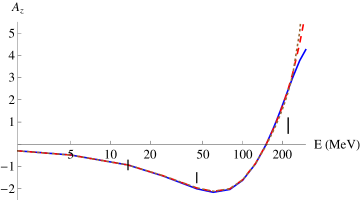
Figure 1: The integrated (angular range $23^{\circ}$ to $52^{\circ}$ (lab)) asymmetry $\bar{A}_{z}$ (in units of $10^{-7}$) as a function of laboratory energy. The energy in MeV is plotted on a logarithmic scale. The blue (solid), red (dashed), and brown (dotted) lines correspond to the different cut-off combinations in Eq. (35). The DDH “best” value, $h_{\pi}=4.6\cdot 10^{-7}$, has been used.

4.1 Fit of the counter term

The calculation of $\bar{A}_{z}(E)$ depends on two unknown LECs: the pion-nucleon coupling constant $h_{\pi}$ and the nucleon-nucleon coupling constant $C$. We require two data points in order to fit both LECs. Before doing so, we first study the results if we use what is known as the DDH “best” value $h_{\pi}=4.6\cdot 10^{-7}$. We fit the LEC $C$ to the central value of the lowest-energy data point. In order to probe the cut-off dependence we perform the fit for three different cut-off combinations (all values in MeV)

$$\{\Lambda,\,\Lambda_{S}\}=\{450,\,500\},\,\{550,\,600\},\,\{600,\,700\}~{},$$ (35)

to obtain the three fits

$$C=\{-4.5,\,-5.1,\,-5.5\}\cdot 10^{-6}~{},$$ (36)

corresponding to cut-off dependence of approximately $10\%$. Using the DDH value for $h_{\pi}$ and the fit values for $C$, the prediction for $\bar{A}_{z}(E)$, integrated from $23^{\circ}$ to $52^{\circ}$, is shown in Fig. 1. First of all, the cut-off dependence of $\bar{A}_{z}$ over the whole relevant energy range is very small, only becoming visible at energies above $221$ MeV. Second, the predictions seem to disagree significantly with the $221$ MeV data point. This, however, is of no concern. The reason being that the measurement at $221$ MeV corresponds to a different angular range which, as we will discuss below, has important consequences. Finally, the predictions somewhat overestimate $|\bar{A}_{z}(45\,\mathrm{MeV})|$. To study this in more detail, we now take the intermediate cut-off combination and fit $C$ to the central value plus or minus one standard deviation of the first data point. We obtain the following fits

$$C=\{-4.3,\,-5.1,\,-6.0\}\cdot 10^{-6}~{}.$$ (37)

The predictions are shown in the left panel of Fig. 2. The second data point is now well described within the experimental uncertainty. Alternatively, we can fit $C$ to the data point at $45$ MeV. Doing so with the intermediate cut-off combination gives the fit

$$C=\{-4.1,\,-4.5,\,-4.9\}\cdot 10^{-6}~{},$$ (38)

and the predictions in the right panel of Fig. 2. Again both low-energy data points are well described within the experimental uncertainty.

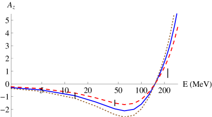
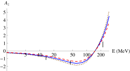
Figure 2: The integrated (angular range $23^{\circ}$ to $52^{\circ}$ (lab)) asymmetry $\bar{A}_{z}$ (in units of $10^{-7}$) as a function of lab energy. The blue (solid), red (dashed), and brown (dotted) lines correspond to a fit to the central value of the first (left plot) or second (right plot) data point, the central value plus one standard deviation, and the central value minus one standard deviation. The intermediate cut-off combination in Eq. (35) has been used and $h_{\pi}=4.6\cdot 10^{-7}$.

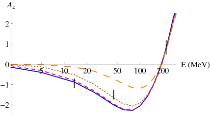
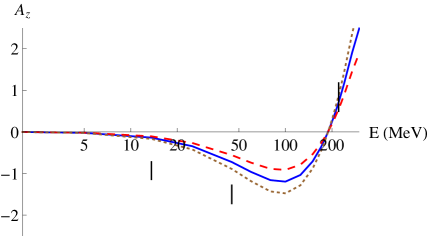
Figure 3: The integrated (angular range $\theta_{c}$ to $90^{\circ}$ (CM frame)) asymmetry $\bar{A}_{z}$ (in units of $10^{-7}$) as a function of lab-energy. Left plot: the blue (solid), red (dashed), brown (dotted), and orange (long-dashed) lines correspond, respectively, to $\theta_{c}=15^{\circ},\,10^{\circ},\,5^{\circ},\,2^{\circ}$. Right plot: The integrated asymmetry with $\theta_{c}=2^{\circ}$. The blue (solid), red (dashed), and brown (dotted) lines correspond to a fit through the first data point plus or minus one standard deviation. In both plots the intermediate cut-off combination has been used and $h_{\pi}=4.6\cdot 10^{-7}$.

In order to include the third data point into the analysis we need to integrate over a different angular range. The experiment at $221$ MeV measures almost the whole cross section apart from scattering under angles smaller than a small critical angle $\theta_{c}$. In the left graph of Fig. 3, we plot $\bar{A}_{z}(E)$ for various values of $\theta_{c}$. We use the intermediate cut-off combination, the DDH best value for $h_{\pi}$, and $C=-5.1\cdot 10^{-6}$ corresponding to a fit to the central value of the first data point. The graphs tells us that at low energies a transmission experiment would be very dependent on the critical angle, but at $221$ MeV there is only a small difference when varying $\theta_{c}$ between $15^{\circ}$ and $2^{\circ}$. These conclusions are in line with the observations made in Refs. [37, 34, 31] where the critical angle behaviour was also studied, albeit for different $P$-even and -odd potentials. With the current fit parameters we predict an asymmetry as measured in the $221$ MeV experiment of

$$6.7\cdot 10^{-8}\leq\bar{A}_{z}(221\,\mathrm{MeV})\leq 7.7\cdot 10^{-8}~{},$$ (39)

in excellent agreement with data. Here the variance, much smaller than the experimental uncertainty, is due to the different choices for $\theta_{c}$.

It should be noted that for $\theta_{c}\geq 10^{\circ}$, the results for $\bar{A}_{z}(13.6\,\mathrm{MeV})$ and $\bar{A}_{z}(45\,\mathrm{MeV})$ are largely insensitive to the angular range as can be seen by comparison of Figs. 1 and 3. At higher energies, varying the angular range has more impact.

In the right panel of Fig. 3, we show $\bar{A}_{z}(E)$ integrated from $2^{\circ}$ to $90^{\circ}$, using the fit values in Eq. (37) for $C$. In order to see how well this fit describes the three data points, one needs to look at this graph for the high-energy data point and the left panel of Fig. 2 for the two low-energy points. The annoyance of having to look at two plots can be avoided by choosing an angular range which corresponds reasonably well to all three data points. As discussed above, the value of $\bar{A}_{z}(E)$ at $13.6$ and $45$ MeV is rather insensitive to the actual angular range as long as the opening angle is larger than $10^{\circ}$, while $\bar{A}_{z}(221\,\mathrm{MeV})$ corresponds very well to the range $10^{\circ}$ to $90^{\circ}$. Using this range we find indeed a good fit to all three data points.

Although the DDH “best” value $h_{\pi}=4.6\cdot 10^{-7}$, accompanied by one four-nucleon operator with the LEC $C\simeq-5.1\cdot 10^{-6}$, describes the existing data satisfactory, this does not imply that these values correspond to the values taken by nature. Taking the lattice-QCD predicted value [26], which agrees with a Skyrme-based prediction [25], $h_{\pi}=1\cdot 10^{-7}$ gives a fit (intermediate cut-off)

$$C=\{-3.2,\,-4.1,\,-4.9\}\cdot 10^{-6}~{},$$ (40)

and predicts asymmetries at $45$ MeV and $221$ MeV of

$$\bar{A}_{z}(45\,\mathrm{MeV})=-(1.9\pm 0.45)\cdot 10^{-7},\qquad\bar{A}_{z}(221\,\mathrm{MeV})=+(0.72\pm 0.16)\cdot 10^{-7}~{},$$ (41)

in agreement with the data, despite a somewhat large prediction of $|\bar{A}_{z}(45\,\mathrm{MeV}|$. At these small values of $h_{\pi}$, $\bar{A}_{z}(E)$ depends dominantly on the counter-term contributions while the TPE contributions are smaller by an order of magnitude.

Finally, rather large values of $h_{\pi}$ are allowed as well. Using $h_{\pi}=1.5\cdot 10^{-6}$, which lies somewhat above the DDH reasonable range, gives the following fit for $C$ (intermediate cut-off)

$$C=\{-7.4,\,-8.3,\,-9.2\}\cdot 10^{-6}~{},$$ (42)

and

$$\bar{A}_{z}(45\,\mathrm{MeV})=-(1.5\pm 0.45)\cdot 10^{-7}~{},\qquad\bar{A}_{z}(221\,\mathrm{MeV})=+(0.54\pm 0.17)\cdot 10^{-7}~{},$$ (43)

again consistent with the data. It should be noted that with these large values for $h_{\pi}$ the cut-off dependence of the results for $\bar{A}_{z}(E)$ becomes significant (approximately $20\%$ at $45$ MeV and $50\%$ at $221$ MeV). This uncertainty is not captured in the error margins of Eq. (43). The increase of the cut-off dependence is due to the larger value of $h_{\pi}$. The counter term only absorbs cut-off dependence in the lowest partial-wave transition ${}^{1}S_{0}\leftrightarrow{}^{3}P_{0}$ while, at higher energies, the TPE potential also contributes to transitions with larger total angular momentum.

What might be surprising is that in the results of Eqs. (41) and (43), the uncertainty of $\bar{A}_{z}(221\,\mathrm{MeV})$ is smaller than that of $\bar{A}_{z}(45\,\mathrm{MeV})$. We will come back to this peculiar behaviour later.

4.2 Fit of both low-energy constants

So far we have been inspired by theoretical estimates of the pion-nucleon coupling constant $h_{\pi}$. However, we have also seen that a relatively large range of values for $h_{\pi}$ describes the data properly, assuming the counter term is fitted to one of the data points. In this section we assume no, a priori, knowledge of $h_{\pi}$ and fit both LECs to the data points. We first fit the LECs to the low-energy data points and predict the third. The reason for fitting first to the low-energy points is that at these energies we can expect our EFT analysis to be most accurate while at higher energies higher-order corrections might start playing a role.

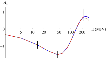
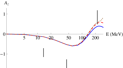
Figure 4: The integrated asymmetry $\bar{A}_{z}$ (in units of $10^{-7}$) as a function of the lab energy (left plots: angular range $23^{\circ}$ to $52^{\circ}$ (lab), right plots: angular range $2^{\circ}$ to $90^{\circ}$ (CM)). The blue (solid), red (dashed), and brown (dotted) lines correspond to the three cut-off combinations in Eq. (35). $h_{\pi}$ and $C$ have been fitted to the central values of the low-energy data points.

Fitting $h_{\pi}$ and $C$ to the central value of the first two data points, while using the three cut-off combinations in Eq. (35), gives the following fits

$$h_{\pi} = \{1.3,\,1.5,\,2.0\}\cdot 10^{-6},$$

$$C = \{-7.5,\,-8.3,\,-10\}\cdot 10^{-6}.$$ (44)

The fit of $h_{\pi}$ is remarkably large with respect to the estimated values and in stark disagreement with the experimental limits given in Sec. 2.1. Before investigating this in more detail, we show the plot of the asymmetry in Fig. 4 for the relevant angular ranges. First of all, we note that the cut-off dependence has increased with respect to the results in Fig. 1 which is due to the increase of $h_{\pi}$. The cut-off dependence is still much smaller than the experimental uncertainty. Secondly, the prediction for the high-energy data point is on the low side but the theoretical and experimental error bands do overlap.

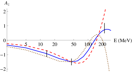
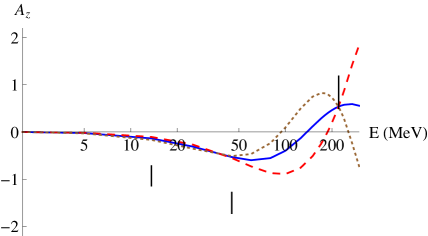
Figure 5: The integrated asymmetry $\bar{A}_{z}$ (in units of $10^{-7}$) as a function of the lab energy (left plots: angular range $23^{\circ}$ to $52^{\circ}$ (lab), right plots: angular range $2^{\circ}$ to $90^{\circ}$ (CM)). The blue (solid), red (dashed), and brown (dotted) lines correspond to the three different fits. For details, see text.

In Fig. 5 we show similar graphs, but we now fitted the LECs to the central value plus or minus one standard deviation of the first data point and the central value of the second data point. The intermediate cut-off combination has been used. The range of the LECs becomes very large

$$h_{\pi} = \{0.14,\,1.5,\,2.8\}\cdot 10^{-6}~{},$$

$$C = \{-3.3,\,-8.3,\,-13\}\cdot 10^{-6}~{},$$ (45)

spanning more than an order of magnitude. The smallest value of $h_{\pi}$ is not far from the experimental limit and rather close to the smaller estimates in Sec. 2.1. Noteworthy is that, despite the huge variance in coupling constants, all three fits almost exactly cross at the energy of the third data point. We will come back to this in detail later.

If we simultaneously vary the second data point by plus or minus one standard deviation and the cut-off combination we obtain the following allowed values

$$h_{\pi} = (1.7\pm 2.5)\cdot 10^{-6}~{},$$

$$C = (-9.3\pm 10)\cdot 10^{-6}~{}.$$ (46)

Here we only give an estimate for the allowed range, in Sec. 4.4 we perform a more detailed analysis. The fits of $h_{\pi}$ and $C$ are, of course, highly correlated which can be seen from the contours in Fig. 8. The fits tell us that small values of $h_{\pi}\sim 10^{-7}$ are not ruled out, however they are definitely not favored. Most fits prefer an $h_{\pi}\sim 10^{-6}$ which is of the order of the NDA estimate but, as mentioned, such values disagree strongly with the experimental upper limits. The cut-off dependence of the fits is modest.

4.3 Crossing points

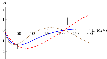
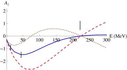
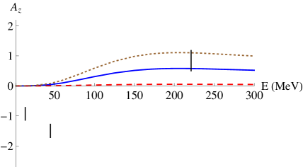
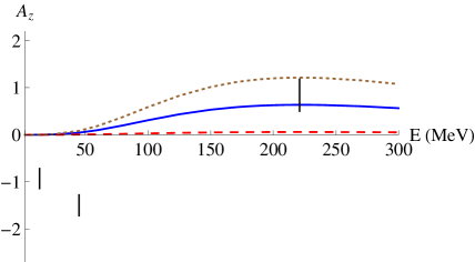
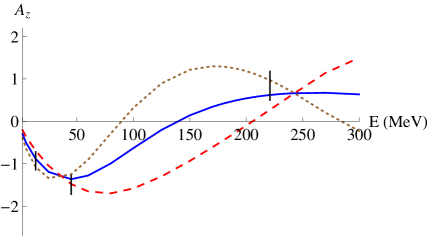
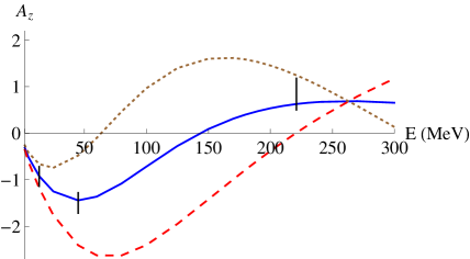
Figure 6: The integrated (angular range $0^{\circ}$ to $90^{\circ}$ (CM frame)) asymmetry $\bar{A}_{z}$ (in units of $10^{-7}$) as a function of the lab energy. The Coulomb amplitude $M_{C}$ is neglected. In the top-plot only $j=0$ $P$-odd transitions are taken into account, in the middle plot all $P$-odd transitions for $0<j\leq 4$, and in the bottom all $P$-odd transition with $j\leq 4$. The plots on the left correspond to the N³LO potential with intermediate cut-off, and the plots on the right to the NijmII potential.

The observation that the three different fits cross in one point in the right plot of Fig. 5 around $220$ MeV is somewhat surprising. In order to understand this behaviour it is useful to dissect the results in terms of different partial-wave contributions. For simplicity we first do the analysis without including the Coulomb amplitude $M_{C}$. In Fig. 6 we use the three fit-values in Eq. (4.2) for the LECs and plot the total asymmetry in the case we neglect $M_{C}$. The plot at the top-left shows the contribution coming from ${}^{1}S_{0}\leftrightarrow{}^{3}P_{0}$ transitions only, the middle-left plot shows the contribution from all $P$-odd transitions with $0<j\leq 4$, and the bottom-left plot shows the complete asymmetry and is, therefore, the sum of the two plots above.

The top-left plot shows that the $j=0$ contributions vanish at an energy of approximately $210$ MeV. This well-known behaviour [37, 42, 34] is due to the vanishing of $\delta_{{}^{1}S_{0}}+\delta_{{}^{3}P_{0}}$ (where $\delta$ denotes the strong phase shifts) at this particular energy. In fact, this zero-crossing was one of the main reasons for the chosen energy of the TRIUMF experiment. It should be noted that the exact point of crossing can vary by $\pm 5$ MeV for the different cut-off combinations. Also, more phenomenological potentials such as the NijmII potential [43] have the zero-crossing around $225$ MeV (see the top-right plot). This dependence on the details of the strong potential already indicates a larger theoretical uncertainty.

The second observation is that between $200$ and $270$ MeV the $j=0$ contributions depends almost linearly on the energy. Around these energies the asymmetry is proportional to

$$\sin(\delta_{{}^{1}S_{0}}-\delta_{{}^{3}P_{0}})\sin(\delta_{{}^{1}S_{0}}+\delta_{{}^{3}P_{0}}+\sigma_{0}+\sigma_{1})\simeq(\delta_{{}^{1}S_{0}}-\delta_{{}^{3}P_{0}})(\delta_{{}^{1}S_{0}}+\delta_{{}^{3}P_{0}})~{},$$ (47)

which indeed shows a linear behaviour from $190$ MeV onwards. Here, we neglected $\sigma_{0}+\sigma_{1}\simeq-0.1^{\circ}$ ($\sigma_{l}$ is defined right below Eq. (24)) which is much smaller than the individual strong phase shifts. The linearity is not affected significantly by the energy dependence of the $P$-odd potentials or total cross section which are fairly constant in this range. Since the $j=0$ contributions depend both on $h_{\pi}$ and $C$, the contributions can be parametrized by

$$\bar{A}_{z}(E)^{i}_{j=0}=(a\,h_{\pi}^{i}+b\,C^{i})(E-E_{0})~{},$$ (48)

where the index $i$ specifies which fit parameters are used, $E_{0}$ is the energy of the zero-crossing point, and $a$ and $b$ are fit-independent constants which can be determined from the slopes of the lines in the top plot. This parametrization only holds in the range where our assumptions regarding the strong phase-shift behaviour hold, which is more-or-less between $200$ and $270$ MeV.

The middle-left plot of Fig. 6 shows that the contributions from the higher partial waves (which are to good approximation dominated by the ${}^{3}P_{2}\leftrightarrow{}^{1}D_{2}$ transitions [34]) are almost constant between $200$ and $270$ MeV, due to the fact that the $j=2$ strong phase-shifts and mixing angle hardly vary over this range. Since the $j>0$ contributions depend only on $h_{\pi}$ the total asymmetry can be parametrized as

$$\bar{A}_{z}(E)^{i}=(a\,h_{\pi}^{i}+b\,C^{i})(E-E_{0})+c\,h_{\pi}^{i}~{},$$ (49)

introducing one more constant $c$ which can be obtained from the height of the lines in the middle plot.

In order to have a crossing point as seen in the bottom-left plot, the following equation should hold for any two fits $i$ and $j$

$$0=\bar{A}_{z}(E_{0}^{\prime})^{i}-\bar{A}_{z}(E_{0}^{\prime})^{j}=[a\,(h_{\pi}^{i}-h_{\pi}^{j})+b\,(C^{i}-C^{j})](E_{0}^{\prime}-E_{0})+c\,(h_{\pi}^{i}-h_{\pi}^{j}),$$ (50)

at a certain energy $E_{0}^{\prime}$. In general, such an equation does not hold for all $i$ and $j$. However, due to the fact that $P$ violation is a perturbative effect, the fitting procedure will always provide a linear relation between the two LECs, as can be clearly seen from the contours in Fig. 8. Using $C^{i}=\alpha h_{\pi}^{i}+\beta$ in Eq. (50), in terms of two new constants, gives

$$0=[a+b\alpha](E_{0}^{\prime}-E_{0})+c~{}.$$ (51)

This relation needs to hold, within the energy range where the approximations are valid, in order for a crossing point to exist. The constants $a$, $b$, and $c$ can be determined from the graphs giving $a\simeq-3.5\cdot 10^{-3}\,\mathrm{MeV}^{-1}$, $b\simeq-6.5\cdot 10^{-4}\,\mathrm{MeV}^{-1}$, and $c\simeq 3.0\cdot 10^{-2}$, while $\alpha\simeq-3.5$ can be obtained from Fig. 8. For these values, we obtain

$$E_{0}^{\prime}-E_{0}\simeq 25\,\mathrm{MeV}~{},$$ (52)

which implies a crossing point at approximately $E_{0}+25\,\mathrm{MeV}\simeq 235\,\mathrm{MeV}$, close to the actual crossing point and within the range where the approximations hold.

The above analysis shows that the existence of crossing point mostly hinges on the energy-dependence of the relevant strong phase shifts. As such, the existence of these points is quite insensitive to the strong potential used as long as it roughly predicts the correct energy scaling of the phase shifts. The actual location of the crossing point, on the other hand, is much more sensitive to details of the potential, in particular to the exact point where $\delta_{{}^{1}S_{0}}+\delta_{{}^{3}P_{0}}=0$, but also on the precise sizes of the phase shifts. To illustrate this, we show the same graphs as before but now using the NijmII potential (note that, for illustrative purposes, we use the same values for $h_{\pi}$ and $C$ and did not refit them), on the right-hand side of Fig. 6. The crossing point still exists, but now appears around $265$ MeV and is shifted by $40$ MeV from $E_{0}\simeq 225\,\mathrm{MeV}$.

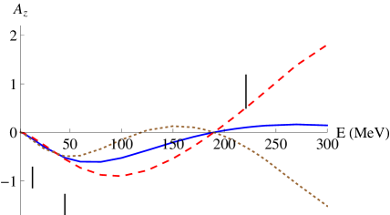
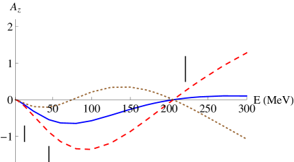
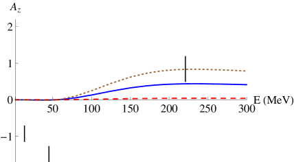
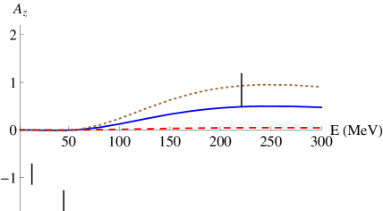
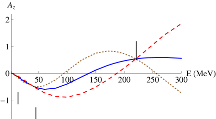
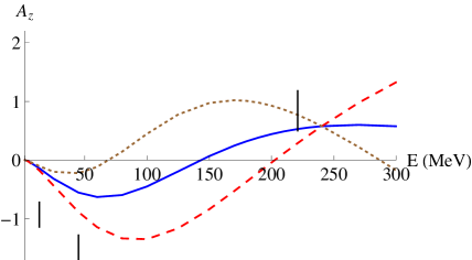
Figure 7: The integrated (angular range $2^{\circ}$ to $90^{\circ}$ (CM frame)) asymmetry $\bar{A}_{z}$ (in units of $10^{-7}$) as a function of the lab energy. The Coulomb amplitude $M_{C}$ is included. In the top-plot only $j=0$ $P$-odd transitions are taken into account, in the middle plot all $P$-odd transitions for $0<j\leq 4$, and in the bottom all $P$-odd transition with $j\leq 4$. The plots on the left correspond to the N³LO potential with intermediate cut-off, and the plots on the right to the NijmII potential.

The analysis so far has neglected the Coulomb amplitude. In Fig. 7, we show the same plots (using the same fits) which do take $M_{C}$ into account. We have used $\theta_{c}=2^{\circ}$ as the critical angle in order to avoid the Coulomb divergence. The plots are very similar to the ones in Fig. 6. The main difference is the location of the zero-crossing points in the plots at the top, and the crossing points in the plots at the bottom. All these points are shifted to lower energies by approximately $20$ MeV. As shown in Refs. [37, 34], introducing the Coulomb amplitude causes the $j=0$ transitions to become proportional to

$$\sin(\delta_{{}^{1}S_{0}}-\delta_{{}^{3}P_{0}})\sin(\delta_{{}^{1}S_{0}}+\delta_{{}^{3}P_{0}}+\sigma_{0}+\sigma_{1}+\phi)~{},$$ (53)

where

$$\phi=2\left[\eta\,\ln(\sin\frac{\theta_{c}}{2})-\sigma_{0}\right]\simeq-4^{\circ},$$ (54)

around $200$ MeV lab energy and using $\theta_{c}=2^{\circ}$. Due to this additional phase, the zero-crossing for $j=0$ contributions is shifted to the energy where $\delta_{{}^{1}S_{0}}+\delta_{{}^{3}P_{0}}=4^{\circ},$ which happens at an energy approximately $20$ MeV lower than the original zero-crossing point at $E_{0}$.

Although the prediction of the total asymmetry is not influenced by a large amount (at least for energies larger than $100$ MeV) by the Coulomb amplitude, as can be seen by comparing the bottom plots in Figs. 6 and 7, the interpretation of the $221$ MeV data point in terms of partial-wave transitions has become murkier. This is best illustrated by looking at the right panels which correspond to the NijmII potential. In the plot without the Coulomb amplitude, the asymmetry is only due to $j>0$ transitions and thus depends only on $h_{\pi}$. This was the reason why the experiment was done at this energy in the first place. The Coulomb amplitude, however, shifts the zero-crossing of the $j=0$ transitions to $205$ MeV which means that the asymmetry at $221$ MeV obtains contributions from $j=0$ and $j>0$ transitions and depends on both $h_{\pi}$ and $C$. The argument that the $221$ MeV is only sensitive to $j>0$ transitions is thus not completely correct once the Coulomb amplitude is included, even if one uses phenomenological potentials which have a phase-shift cancellation at this energy. Of course, the same analysis holds for the chiral potential, but in this case the asymmetry at $221$ MeV already depends on both $j=0$ and $j>0$ transitions before including the Coulomb amplitude.

The fact that, once the Coulomb amplitude has been included, the crossing point for the chiral potential lies almost exactly at the energy of the third data point, should be seen as a coincidence. Nevertheless, the observation that, in general, the crossing point lies very close to the third data point implies that this point has less discriminating power with respect to the fit parameters than might be expected. Furthermore, the sensitivity to details of the strong interaction potential combined with the knowledge that the chiral potentials are not very accurate at these energies, means that this data point is hard to analyze in our EFT framework.

4.4 Fit through all data points

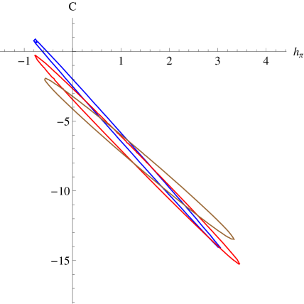
Figure 8: Contours of constant $\chi^{2}$ in the $h_{\pi}-C$ plane (both in units of $10^{-6}$). The left plot shows contours of total $\chi^{2}=1,\,2,\,3,\,4$ for the intermediate cut-off combination, while the right plot shows contours of total $\chi^{2}=2.71$ for the three different cut-off combinations.

Despite the issues raised in the previous section related to the data point at $221$ MeV, it is still interesting to investigate a fit through all points. In the left part of Fig. 8, we plot contours of constant total $\chi^{2}=1,\,2,\,3,\,4$ using the intermediate cut-off combination. In the right part we study the cut-off dependence of the fit by plotting contours of constant total $\chi^{2}=2.71$ for the three different cut-off combinations.

From the right plot it becomes clear that the cut-off dependence of the fit is small since the contours mostly overlap. Second, the left plot shows that at the level of total $\chi^{2}=1$ the contour does not include small values of $h_{\pi}\sim 10^{-7}$ which are favored by theory [24, 25, 26] and the experimental data on ${}^{18}F$ $\gamma$-ray emission [27, 28]. However, these values are already included at the level of total $\chi^{2}=2$ and we conclude that our analysis of the longitudinal asymmetry is consistent with such small values of $h_{\pi}$. Clearly, our analysis allows for much larger (and smaller) values of $h_{\pi}$ as well and more data is needed to further pinpoint the size of this important LEC. All in all, the allowed range for the LECs, at the total $\chi^{2}=2.71$ level, is approximately

$$h_{\pi} = (1.1\pm 2)\cdot 10^{-6}~{},$$

$$C = (-6.5\pm 8)\cdot 10^{-6}~{}.$$ (55)

Although the uncertainties of the fit are reduced compared to Eq. (4.2), the reduction is smaller than might be expected due to the existence of the crossing points.

With the latter comments in mind, it becomes interesting to study at which energies a new experiment would have most impact. A smaller energy than $221$ MeV is preferred because at lower energies the chiral potentials are more reliable. Simultaneously, the energy should be significantly higher than $45$ MeV in order not to overlap with the PSI experiment. An experiment at a lab energy between $100$ and $150$ MeV seems to be best suited. These energies have the major advantage over $221$ MeV that they are sufficiently far from the crossing points.

Apart from the energy, the angular range is also of importance [37, 34]. By looking at Fig. 5, we see that a larger angular range has more discriminating power. On the other hand, the opening angle needs to be big enough such that there is no large sensitivity to small variations in $\theta_{c}$. It seems an experiment measuring from $10^{\circ}$ to $80^{\circ}$ (lab coordinates) combines the best of both worlds.

5 Discussion and conclusions

Historically, parity violation in hadronic processes has mostly been discussed in the one-boson-exchange framework of DDH [1]. In this framework, parity violation arises due to the single exchange of a pion, $\rho$- or $\omega$-meson. In the chiral EFT approach we adopt here, the exchange of the heavy mesons are captured by four-nucleon contact interactions. One-pion exchange appears in both the DDH and the chiral EFT framework, however, in the latter, at the same order as the contact interactions, there are contributions due to two-pion-exchange diagrams [8, 9]. Due to its isospin properties one-pion exchange vanishes in $pp$ scattering. In the DDH framework the longitudinal asymmetry does therefore not depend on the weak pion-nucleon coupling constant $h_{\pi}$. Consequently, this important LEC has been often neglected in calculations of the longitudinal asymmetry. A proper low-energy description of hadronic parity violation contains two-pion-exchange diagrams which do contribute to the asymmetry in $pp$ scattering. These contributions have so far been investigated in a hybrid approach in Refs. [30, 31], but the authors of these references did not extract the value of $h_{\pi}$.

In this work, we reinvestigated the asymmetry in $pp$ scattering in chiral effective field theory. For the $P$-conserving $N\!N$ potential we used the N³LO potential obtained from chiral effective field theory [20] and, within the same power-counting scheme, the $P$-violating potential up to NLO. Both potentials are systematically regularized and theoretical errors due to cut-off dependence have been investigated and found to be negligible at low energies. At higher energies the uncertainty grows but is still much smaller than experimental errors.

We have found that the $P$-odd NLO potential, consisting of TPE contributions and one four-nucleon contact term, successfully describes the existing data. The two unknown LECs can be fitted to the data at $13.6$ and $45$ MeV, and the third data point at $221$ MeV can be predicted. Unfortunately, our analysis has shown that, due to the particular energy-dependence of the strong phase shifts and the $P$-odd potential, different fits for the unknown LECs predict more-or-less similar asymmetries around $221$ MeV. This behaviour limits the discriminating power of the $221$ MeV data point and forces us to adopt a rather large allowed range for $h_{\pi}$ and $C$.

The allowed range for $h_{\pi}=(1.1\pm 2)\cdot 10^{-6}$ is consistent with the experimental limits obtained from $\gamma$-ray emission of ${}^{18}F$ and with theoretical estimations. However, it is clear that more experimental data is needed to reduce the uncertainty on $h_{\pi}$. Our analysis shows that an additional measurement of the asymmetry in the energy range of $100$ to $150$ MeV would be beneficial. This energy has some advantages over the $221$ MeV data point. The most important ones being that the chiral potentials (both the $P$-conserving and $P$-violating) are more accurate at lower energies and that such energies are sufficiently far away from the crossing points discussed in Sec. 4.3.

Additional input can, of course, come from other observables than the $pp$ longitudinal asymmetry. In particular, the angular asymmetry in $\vec{n}p\rightarrow d\gamma$ is a very promising observable although, so far, there only exists an experimental upper bound. A major advantage of this observable is that, in contrast with the $pp$ asymmetry, it does depend on the LO $P$-odd potential and thus cleanly probes $h_{\pi}$ [44]. A caveat is that, if $h_{\pi}$ is really as small as suggested, this observable might also obtain important contributions from higher-order corrections in the form of parity-violating four-nucleon contact or nucleon-pion-photon interactions. We plan to investigate this observable in our chiral-EFT approach in future work.

The allowed range for $C=(-6.5\pm 8)\cdot 10^{-6}$ is harder to compare with existing literature in which these contributions are usually described via $\rho$- and $\omega$-meson exchange. The $pp$ asymmetry is typically expressed in terms of two independent combinations (one for the ${}^{1}S_{0}-{}^{3}P_{0}$ transition and one for the ${}^{3}P_{2}-{}^{1}D_{2}$ transition) of DDH couplings [2]. By application of resonance-saturation methods these approaches can be compared, but one must be careful to not double count the TPE contributions (for details, see Refs. [45, 46]). Here we refrain from a detailed comparison. Instead, we compare our results to the calculation in pionless EFT [13]. In this framework pions are integrated out and $P$-odd interactions are fully described by contact interactions among nucleons and, as such, the asymmetry in $pp$ scattering depends on only one LEC, in the notation of Ref. [13], $\mathcal{A}_{pp}$. The authors performed an analysis of the data points at $13.6$ and $45$ MeV and found $\mathcal{A}_{pp}=(1.3\pm 0.3)\cdot 10^{-14}\,\mathrm{MeV}^{-3}$. In order to compare to the pionless approach we should set $h_{\pi}=0$. From Fig. 8 we infer that this means $C=-(3.0\pm 1.0)\cdot 10^{-6}$, in order to describe the data. Translating this to the notation of Ref. [13] we obtain a value for $\mathcal{A}_{pp}$

$$\mathcal{A}_{pp}=-\frac{C}{2F_{\pi}\Lambda_{\chi}^{2}}=(1.6\pm 0.5)\cdot 10^{-14}\,\mathrm{MeV}^{-3},$$ (56)

in good agreement with the pionless result. Of course, non-vanishing values of $h_{\pi}$ can give very different values for $C$. Notice further that the above comparison should not be taken too seriously since the LEC $C$ we consider in this work is, strictly speaking, a bare quantity. On the other hand, the quoted value for $\mathcal{A}_{pp}$ corresponds to a renormalized LEC at the scale $\mu=m_{\pi}$.

As mentioned, more experimental data is needed to further constrain the LECs. If additional data is at odds with our allowed ranges for $h_{\pi}$ and $C$, for example if upcoming experiments on the angular asymmetry in $\vec{n}p\rightarrow d\gamma$ find a value of $h_{\pi}\sim 10^{-7}$ while, simultaneously, a new experiment on the $pp$ asymmetry constrains $h_{\pi}\sim 10^{-6}$, it might be that higher-order corrections to the $P$-odd potential need to be taken into account. In fact, by analogy to the $P$-conserving case where next-to-next-to-leading order (N²LO) and N³LO contributions are very relevant, this might be expected. On the other hand, the analysis of Ref. [9] shows that certain corrections to the TPE-diagrams, which are important for the $P$-conserving potential, are small in the $P$-violating case. A full calculation of the N²LO $P$-odd potential is necessary to say more about this potential issue.

In summary, we have investigated the longitudinal asymmetry in proton-proton scattering in chiral effective field theory. We calculated the asymmetry up to next-to-leading order in the parity-violating potential. By a careful comparison with the experimental data we have extracted allowed ranges for the two relevant parity-odd low-energy constants. The allowed ranges are consistent with theoretical calculations of the LECs and with experimental limits. However, more data is required in order to extract preciser values of the coupling constants.

Acknowledgements

We thank Andreas Nogga for many helpful comments and discussions, Dieter Eversheim for providing helpful information about details of the Bonn experiment, and Matthias Schindler for clarifications of the pionless calculation. This work is supported in part by the DFG and the NSFC through funds provided to the Sino-German CRC 110 “Symmetries and the Emergence of Structure in QCD”, by the EU (HadronPhysics3) and ERC project 259218 NUCLEAREFT.

Appendix A Partial-wave decomposition of the $P$-odd potential

In order to solve the LS equation, it is necessary to have a partial wave decomposition of the potential. Details on the decomposition of the $P$-even potential can be found in Ref. [20] and here we consider the $P$-odd potential. Let us first ignore isospin, we then need to decompose a potential of the form

$$V=i(\vec{\sigma}_{1}\times\vec{\sigma}_{2})\cdot\vec{q}\,f(q)~{},$$ (57)

where the form of $f(q)$ depends on whether we look at the TPE or the contact potential. Apart from isospin we have

$$V^{l^{\prime}l\,s^{\prime}s}_{j}(p^{\prime},p) = \langle p^{\prime}\,(l^{\prime}s^{\prime})j||V||p\,(ls)j\rangle$$ (58)

$$= -216\pi\sum_{k}\hat{k}^{3/2}(-1)^{k}g_{k}(q)\!\!\!\sum_{\lambda_{1}+\lambda_{2}=1}\sqrt{\frac{\hat{\lambda}_{1}\hat{\lambda}_{2}}{\hat{\lambda}_{1}!\hat{\lambda}_{2}!}}(p)^{\lambda_{1}}(-p^{\prime})^{\lambda_{2}}$$

$$\times C(\lambda_{1}\,k\,l;000)\,C(\lambda_{2}\,k\,l^{\prime};000)\begin{pmatrix}\lambda_{1}&\lambda_{2}&1\\ k&k&0\\ l&l^{\prime}&1\end{pmatrix}$$

$$\times(-1)^{l}\sqrt{\hat{s}\hat{s^{\prime}}\hat{j}}\begin{pmatrix}l^{\prime}&\l&1\\ s^{\prime}&s&1\\ j&j&0\end{pmatrix}\begin{pmatrix}1/2&1/2&1\\ 1/2&1/2&1\\ s^{\prime}&s&1\end{pmatrix}~{},$$

where $\hat{x}=2x+1$ and

$$g_{k}(q)=\int_{-1}^{1}dx^{\prime}\,P_{k}(x^{\prime})f(q(x^{\prime}))~{},$$ (59)

in terms of $q^{2}(x^{\prime})=p^{2}+p^{\prime\,2}-2pp^{\prime}x^{\prime}$ and $P_{k}(x^{\prime})$ are the Legendre polynomials. To be specific, for the TPE potential

$$f(q(x^{\prime}))=\frac{1}{(2\pi)^{3}}V_{\text{TPE}}(q^{\prime},\Lambda_{S})e^{-p^{6}/\Lambda^{6}}e^{-p^{\prime\,6}/\Lambda^{6}}~{}.$$

To include isospin, we should multiply by the following factor

$$\langle(\frac{1}{2}\frac{1}{2})t^{\prime}m_{t}^{\prime}|(\vec{\tau}_{1}+\vec{\tau}_{2})^{3}|(\frac{1}{2}\frac{1}{2})tm_{t}\rangle = C(t\,1\,t^{\prime};m_{t}\,0\,m_{t}^{\prime})\langle(\frac{1}{2}\frac{1}{2})t^{\prime}m_{t}^{\prime}||(\vec{\tau}_{1}+\vec{\tau}_{2})^{3}||(\frac{1}{2}\frac{1}{2})tm_{t}\rangle$$ (60)

$$= C(t\,1\,t^{\prime};m_{t}\,0\,m_{t}^{\prime})6\sqrt{\hat{t}}\,[1+(-1)^{t+t^{\prime}}]\begin{pmatrix}1/2&1/2&1\\ 1/2&1/2&0\\ t^{\prime}&t&1\end{pmatrix}.$$

In the case of proton-proton scattering we can put $t^{\prime}=t=m_{t}^{\prime}=m_{t}=1$.

Appendix B Solution of the LS equation in momentum space

There are two main ways of approaching the problem in the sense that we can treat the $P$-odd potential either perturbatively or nonperturbatively. We begin with the latter approach. The first step involves the removal of the $i\epsilon$ in the numerator by writing

$$\frac{1}{E-p^{\prime\prime\,2}/m_{p}+i\epsilon}=\frac{m_{p}}{q_{0}^{2}-p^{\prime\prime\,2}+i\epsilon}=\frac{m_{p}}{q_{0}+p^{\prime\prime}}\left(\frac{\mathcal{P}}{q_{0}-p^{\prime\prime}}-i\pi\delta(q_{0}-p^{\prime\prime})\right)~{},$$

where $\mathcal{P}$ denotes the principal value integral, and $E=q_{0}^{2}/m_{p}$ such that $q_{0}$ is the on-shell momentum. We can now write the LS equation as

$$T^{l^{\prime}l\,s^{\prime}s}_{j}(p^{\prime},p,E) = V^{l^{\prime}l\,s^{\prime}s}_{j}(p^{\prime},p)+m_{p}\sum_{l^{\prime\prime}\,s^{\prime\prime}}\mathcal{P}\!\!\int_{0}^{p_{\mathrm{max}}}dp^{\prime\prime}\,V^{l^{\prime}l^{\prime\prime}\,s^{\prime}s^{\prime\prime}}_{j}(p^{\prime},p^{\prime\prime})\frac{p^{\prime\prime\,2}}{q_{0}^{2}-p^{\prime\prime\,2}}T^{l^{\prime\prime}l\,s^{\prime\prime}s}_{j}(p^{\prime\prime},p,E)$$ (61)

$$-i\frac{\pi m_{p}q_{0}}{2}\sum_{l^{\prime\prime}\,s^{\prime\prime}}V^{l^{\prime}l^{\prime\prime}\,s^{\prime}s^{\prime\prime}}_{j}(p^{\prime},q_{0})T^{l^{\prime\prime}l\,s^{\prime\prime}s}_{j}(q_{0},p,E)~{},$$

where we introduced $p_{\mathrm{max}}\gg\Lambda$ which corresponds to the final grid point used in the numerical solution. We now subtract the divergence in the first integral and add it back again and write

$$T^{l^{\prime}l\,s^{\prime}s}_{j}(p^{\prime},p,E) = V^{l^{\prime}l\,s^{\prime}s}_{j}(p^{\prime},p)$$ (62)

$$+m_{p}\sum_{l^{\prime\prime}\,s^{\prime\prime}}\int_{0}^{p_{\mathrm{max}}}dp^{\prime\prime}\,\bigg{[}V^{l^{\prime}l^{\prime\prime}\,s^{\prime}s^{\prime\prime}}_{j}(p^{\prime},p^{\prime\prime})\frac{p^{\prime\prime\,2}}{q_{0}^{2}-p^{\prime\prime\,2}}T^{l^{\prime\prime}l\,s^{\prime\prime}s}_{j}(p^{\prime\prime},p,E)$$

$$-V^{l^{\prime}l^{\prime\prime}\,s^{\prime}s^{\prime\prime}}_{j}(p^{\prime},q_{0})\frac{q_{0}^{2}}{q_{0}^{2}-p^{\prime\prime\,2}}T^{l^{\prime\prime}l\,s^{\prime\prime}s}_{j}(q_{0},p,E)\bigg{]}$$

$$+m_{p}q_{0}^{2}V^{l^{\prime}l^{\prime\prime}\,s^{\prime}s^{\prime\prime}}_{j}(p^{\prime},q_{0})T^{l^{\prime\prime}l\,s^{\prime\prime}s}_{j}(q_{0},p,E)\mathcal{P}\!\!\int_{0}^{p_{\mathrm{max}}}dp^{\prime\prime}\frac{1}{q_{0}^{2}-p^{\prime\prime\,2}}$$

$$-i\frac{\pi m_{p}q_{0}}{2}\sum_{l^{\prime\prime}\,s^{\prime\prime}}V^{l^{\prime}l^{\prime\prime}\,s^{\prime}s^{\prime\prime}}_{j}(p^{\prime},q_{0})T^{l^{\prime\prime}l\,s^{\prime\prime}s}_{j}(q_{0},p,E)~{},$$

where the first integral has no pole so the principal value has been removed. The second integral can be done analytically and gives

$$\mathcal{P}\!\!\int_{0}^{p_{\mathrm{max}}}dp^{\prime\prime}\frac{1}{q_{0}^{2}-p^{\prime\prime\,2}}=\frac{1}{2q_{0}}\ln\frac{p_{\mathrm{max}}+q_{0}}{|p_{\mathrm{max}}-q_{0}|}~{}.$$

The LS equation can now be solved numerically. The main difference with respect to only strong interactions is that more channels are coupled. Where in the limit of no parity violation (and isospin violation) there are two coupled and two uncoupled channels, in this case there are in general four coupled channels. In the case of $pp$ scattering there are always less channels (two coupled channels if $j=0$, one uncoupled channel if $j$ is odd, and three coupled channels if $j>0$ and even). In general, we solve the whole $T$-matrix at once. We write it as

$$T^{l^{\prime}l\,s^{\prime}s}_{j}=\begin{pmatrix}T^{j-1\,j-1\,11}_{j}&T^{j-1\,j+1\,11}_{j}&T^{j-1\,j\,11}_{j}&T^{j-1\,j\,10}_{j}\\ T^{j+1\,j-1\,11}_{j}&T^{j+1\,j+1\,11}_{j}&T^{j+1\,j\,11}_{j}&T^{j+1\,j\,10}_{j}\\ T^{j\,j-1\,11}_{j}&T^{j\,j+1\,11}_{j}&T^{j\,j\,11}_{j}&T^{j\,j\,10}_{j}\\ T^{j\,j-1\,01}_{j}&T^{j\,j+1\,01}_{j}&T^{j\,j\,01}_{j}&T^{j\,j\,00}_{j}\end{pmatrix}~{}.$$ (63)

The top-left $2\times 2$ matrix corresponds to the “standard” coupled channels and the $33$ and $44$ entries are the “standard” uncoupled channels. The entries connecting $j$ and $j\pm 1$ are zero in the absence of parity violation. The entries $T^{j\,j\,10}_{j}$ and $T^{j\,j\,01}_{j}$ remain zero unless there is isospin violation which changes total isospin in the strong interaction.

The other option is to solve the LS equation perturbatively. Ignoring all indices, the LS equation becomes

$$T=V+VG_{0}T~{},$$

where $V=V_{P}+V_{/P}$, with $V_{P}$ denoting the $P$-conserving potential and $V_{/P}$ the $P$-violating potential. If we treat $V_{/P}$ as a perturbation we can use first-order perturbation theory and write $T=T_{P}+T_{/P}$ as well. The leading equation becomes

$$T_{P}=V_{P}+V_{P}G_{0}T_{P}~{}.$$

This is just the ordinary strong LS equation which can be solved with the methods described above. The first-order equation becomes

$$T_{/P}=V_{/P}+V_{P}G_{0}T_{/P}+V_{/P}G_{0}T_{P}\qquad\rightarrow\qquad(1-V_{P}G_{0})T_{/P}=V_{/P}+V_{/P}G_{0}T_{P}~{}.$$

The leading-order equation can be rewritten into

$$1-V_{P}G_{0}=(1+T_{P}G_{0})^{-1}$$

such that

$$T_{/P}=(1+T_{P}G_{0})(V_{/P}+V_{/P}G_{0}T_{P})=V_{/P}+V_{/P}G_{0}T_{P}+T_{P}G_{0}V_{/P}+T_{P}G_{0}V_{/P}G_{0}T_{P}~{},$$ (64)

which can be solved directly. We have checked explicitly that the perturbative and the nonperturbative treatments give the same solution for the $T$-matrix, if the $P$-odd potential is small enough.

References

- [1] B. Desplanques, J. F. Donoghue and B. R. Holstein, Annals Phys. 124 (1980) 449.
- [2] W. C. Haxton and B. R. Holstein, Prog. Part. Nucl. Phys. 71 (2013) 185.
- [3] M. R. Schindler and R. P. Springer, Prog. Part. Nucl. Phys. 72 (2013) 1.
- [4] V. Bernard and U.-G. Meißner, Ann. Rev. Nucl. Part. Sci. 57 (2007) 33.
- [5] E. Epelbaum, H.-W. Hammer and U.-G. Meißner, Rev. Mod. Phys. 81 (2009) 1773.
- [6] R. Machleidt and D. R. Entem, Phys. Rept. 503 (2011) 1.
- [7] D. B. Kaplan and M. J. Savage, Nucl. Phys. A 556 (1993) 653 [Erratum-ibid. A 570 (1994) 833] [Erratum-ibid. A 580 (1994) 679].
- [8] S.-L. Zhu, C. M. Maekawa, B. R. Holstein, M. J. Ramsey-Musolf and U. van Kolck, Nucl. Phys. A 748 (2005) 435.
- [9] N. Kaiser, Phys. Rev. C 76 (2007) 047001.
- [10] M. J. Savage and R. P. Springer, Nucl. Phys. A 644 (1998) 235 [Erratum-ibid. A 657 (1999) 457].
- [11] M. J. Savage, Nucl. Phys. A 695 (2001) 365.
- [12] L. Girlanda, Phys. Rev. C 77 (2008) 067001.
- [13] D. R. Phillips, M. R. Schindler and R. P. Springer, Nucl. Phys. A 822 (2009) 1.
- [14] B. R. Holstein, Eur. Phys. J. A 41 (2009) 279.
- [15] C. Ordonez, L. Ray and U. van Kolck, Phys. Rev. Lett. 72 (1994) 1982.
- [16] C. Ordonez, L. Ray and U. van Kolck, Phys. Rev. C 53 (1996) 2086.
- [17] E. Epelbaum, W. Glöckle and U.-G. Meißner, Nucl. Phys. A 637 (1998) 107.
- [18] E. Epelbaum, W. Glöckle and U.-G. Meißner, Nucl. Phys. A 671 (2000) 295.
- [19] D. R. Entem and R. Machleidt, Phys. Rev. C 68 (2003) 041001.
- [20] E. Epelbaum, W. Glöckle and U.-G. Meißner, Nucl. Phys. A 747 (2005) 362.
- [21] E. Epelbaum, W. Glöckle and U.-G. Meißner, Eur. Phys. J. A 19 (2004) 125.
- [22] A.V. Manohar and H. Georgi, Nucl. Phys. B 234 (1984) 189.
- [23] H. Georgi and L. Randall, Nucl. Phys. B 276 (1986) 241.
- [24] N. Kaiser and U.-G. Meißner, Nucl. Phys. A 499 (1989) 699.
- [25] U.-G. Meißner and H. Weigel, Phys. Lett. B 447 (1999) 1.
- [26] J. Wasem, Phys. Rev. C 85 (2012) 022501.
- [27] E. G. Adelberger, M. M. Hindi, C. D. Hoyle, H. E. Swanson, R. D. Von Lintig and W. C. Haxton, Phys. Rev. C 27 (1983) 2833.
- [28] S. A. Page, H. C. Evans, G. T. Ewan, S. P. Kwan, J. R. Leslie, J. D. Macarthur, W. Mclatchie and P. Skensved et al., Phys. Rev. C 35 (1987) 1119.
- [29] W. C. Haxton, Phys. Rev. Lett. 46 (1981) 698.
- [30] C.-P. Liu, Phys. Rev. C 75 (2007) 065501.
- [31] T. M. Partanen, J. A. Niskanen and M. J. Iqbal, Eur. Phys. J. A 48 (2012) 119.
- [32] C. M. Vincent and S. C. Phatak, Phys. Rev. C 10 (1974) 391.
- [33] M. Walzl, U.-G. Meißner and E. Epelbaum, Nucl. Phys. A 693 (2001) 663.
- [34] J. Carlson, R. Schiavilla, V. R. Brown and B. F. Gibson, Phys. Rev. C 65 (2002) 035502.
- [35] X. Kong and F. Ravndal, Nucl. Phys. A 665 (2000) 137.
- [36] J. R. Taylor, Scattering Theory, (Dover Publications, 2006).
- [37] D. E. Driscoll and G. A. Miller, Phys. Rev. C 39 (1989) 1951.
- [38] P. D. Eversheim, W. Schmitt, S. E. Kuhn, F. Hinterberger, P. von Rossen, J. Chlebek, R. Gebel and U. Lahr et al., Phys. Lett. B 256 (1991) 11.
- [39] P. D. Eversheim, private communication.
- [40] S. Kistryn, J. Lang, J. Liechti, T. Maier, R. Muller, F. Nessi-Tedaldi, M. Simonius and J. Smyrski et al., Phys. Rev. Lett. 58 (1987) 1616.
- [41] A. R. Berdoz et al. [TRIUMF E497 Collaboration], Phys. Rev. Lett. 87 (2001) 272301.
- [42] D. E. Driscoll and U.-G. Meißner, Phys. Rev. C 41 (1990) 1303.
- [43] V. G. J. Stoks, R. A. M. Klomp, C. P. F. Terheggen and J. J. de Swart, Phys. Rev. C 49 (1994) 2950.
- [44] D. B. Kaplan, M. J. Savage, R. P. Springer and M. B. Wise, Phys. Lett. B 449 (1999) 1.
- [45] E. Epelbaum, U.-G. Meißner, W. Glöckle and C. Elster, Phys. Rev. C 65 (2002) 044001.
- [46] J. C. Berengut, E. Epelbaum, V. V. Flambaum, C. Hanhart, U.-G. Meißner, J. Nebreda and J. R. Pelaez, Phys. Rev. D 87 (2013) 085018.