RUNHETC-2013-15

Classical Conformal Blocks and Painlevé VI

Alexey Litvinov¹, Sergei Lukyanov¹,
Nikita Nekrasov${}^{2,\,3^{*},\,4^{*},\,5^{*}}$ and Alexander Zamolodchikov${}^{1^{*},\,3}$

$\ {}^{1}$NHETC, Department of Physics and Astronomy, Rutgers University,

Piscataway, NJ 08855-0849, USA

² Simons Center for Geometry and Physics, Stony Brook, NY 11794-3636, USA

³ Institut des Hautes Etudes Scientifiques, Bures-sur-Yvette 91440, France

⁴ Kharkevich Institute for Information Transmission Problems, Lab. 5, Moscow 127994 Russia

⁵ Alikhanov Institute of Theoretical and Experimental Physics, Moscow 117218, Russia

Abstract

We study the classical $c\to\infty$ limit of the Virasoro conformal blocks. We point out that the classical limit of the simplest nontrivial null-vector decoupling equation on a sphere leads to the Painlevé VI equation. This gives the explicit representation of generic four-point classical conformal block in terms of the regularized action evaluated on certain solution of the Painlevé VI equation. As a simple consequence, the monodromy problem of the Heun equation is related to the connection problem for the Painlevé VI.

 

^∗ On leave of absence

1 Introduction

Originally, conformal blocks were introduced in the context of two dimensional conformal field theories [1], where they play fundamental role in the holomorphic factorization of the correlation functions. More recently, these functions attracted renewed attention because of their remarkable relation to the correlators of supersymmetry-protected chiral operators in the ${\mathcal{N}}=2$ supersymmetric gauge theories in four dimensions. This relation, dubbed the BPS/CFT correspondence in [2], following the prior work in [3, 4, 5], became a subject of intense development after the seminal work [6] where the instanton partition functions of the $\mathcal{S}$-class $\mathcal{N}=2$ gauge theories in the $\Omega$-background [3] were conjectured to be the Liouville (and, more generally, the $ADE$ Toda) conformal blocks.

The conformal blocks are fully determined by their defining properties (the conformal symmetry in CFT, and, for the quiver gauge theories, the instanton integrals of the supersymmetric gauge theories). However, apart from (numerous) special cases, no closed form expressions are known beyond the power series expansions. Therefore, any relations which could provide an additional analytic control are of interest. In this note we establish a relation between the so-called classical conformal blocks [7, 8] and the classical action evaluated on the special solutions of the celebrated Painlevé VI equation.

Generally, the conformal blocks are associated with the moduli spaces ${\mathcal{M}}_{g,n}$ of genus $g$ Riemann surfaces with $n$ punctures. In the present note we limit our attention to the $n$-punctured spheres (and ultimately our result will be concerned with the simplest nontrivial case $n=4$). Loosely speaking, the conformal blocks are $n$-point correlation functions $\langle\,V_{\Delta_{1}}(z_{1})\cdots V_{\Delta_{n}}(z_{n})\,\rangle$ of the chiral primary operators $V_{\Delta}(z)$. The subscripts $\Delta$ indicate the associated conformal dimensions. Since generally the chiral primaries are not local fields, the notion of their correlation functions is ambiguous. Actual conformal blocks are defined relative to a given “pant decomposition” of the $n$-punctured sphere, usually represented by a “dual diagram”. For example, the diagram in Fig. 1

\psfrag{z1}{$z_{1},\Delta_{1}$}\psfrag{z2}{$z_{2},\Delta_{2}$}\psfrag{z3}{$z_{n-1},\Delta_{n-1}$}\psfrag{z4}{$z_{n},\Delta_{n}$}\psfrag{p1}{$\Delta(P_{1})$}\psfrag{p2}{$\Delta(P_{2})$}\psfrag{p3}{$\Delta(P_{n-3})$}\includegraphics[width=398.33858pt]{paint.eps}

Figure 1: Dual diagram representing the “pant decomposition” of $n$-punctured sphere for the conformal block (1.1). The external legs are associated with the insertions $V_{\Delta_{i}}(z_{i}),\ i=1,...,n$, while the internal links represent the intermediate spaces with the primary dimensions $\Delta(P_{\alpha})$. The vertices correspond to the elementary three-punctured spheres of the given pant decomposition.

represents the instruction to include only the states from the irreducible representations with the conformal weights $\Delta(P_{\alpha})$ in the intermediate-state decompositions of the operator product,

$$\mathcal{F}_{\bf P}({\bf z})=\langle\,V_{\Delta_{1}}(z_{1})\Pi_{\Delta(P_{1})}V_{\Delta_{2}}(z_{2})\Pi_{\Delta(P_{2})}\cdots\Pi_{\Delta(P_{n-3})}V_{\Delta_{n}}(z_{n})\,\rangle\,,$$ (1.1)

where $\Pi_{\Delta(P)}$ stand for the projection operators. (In what follows we often omit the projection operators and just refer to the associated dual diagram.) Here and below we use the Liouville-inspired parameterization of the “intermediate” dimensions $\Delta(P)$ and the Virasoro central charge $c$,

$$\Delta(P)=\frac{c-1}{24}+P^{2}\,,\qquad c=1+6\,(b+b^{-1})^{2}\,.$$ (1.2)

Thus, the $n$-point conformal block depends on $n-3$ parameters ${\bf P}=\{P_{1},P_{2},\ldots P_{n-3}\}$. Although the definition (1.1) involves $n$ points $z_{1},\ldots z_{n}$, projective transformations allow one to fix three of them, e.g. by sending the three points, say $z_{n-2},\ z_{n-1},\ z_{n}$, to the standard locations $0,\ 1$ and $\infty$. Therefore, the conformal block (1.1) depends on $n-3$ moduli, which we collectively denote by ${\bf z}=\{z_{1},\ldots z_{n-3}\}$. Although the conformal block also depends on $n$ “external leg” dimensions $\Delta_{1},\Delta_{2},\ldots\Delta_{n}$, we omit these parameters in the above notation $\mathcal{F}_{\bf P}({\bf z})$. In the simplest nontrivial case $n=4$ there is only one complex modulus. In this special case we fix the coordinate $x$ on the moduli space ${\mathcal{M}}_{0,4}$ by setting

$$\{z_{1},\,z_{2},\,z_{3},\,z_{4}\}=\{0,\,x,\,1,\,\infty\}\,.$$ (1.3)

Also, there is only one intermediate state parameter, the momentum $P$. Suppressing again the dependence on $\Delta_{i},\ i=1,\ldots,4$, we denote by $\mathcal{F}_{P}(x)$ the $4$-point conformal block associated with the dual diagram in Fig. 2.

\psfrag{z1}{$0,\Delta_{1}$}\psfrag{z2}{$x,\Delta_{2}$}\psfrag{z3}{$\Delta(P)$}\psfrag{z4}{$1,\Delta_{3}$}\psfrag{z5}{$\infty,\Delta_{4}$}\includegraphics[width=284.52756pt]{paint4.eps}

Figure 2: The dual diagram representation of the four-point conformal block $\mathcal{F}_{P}(x)$.

The conformal properties allow one to determine, in principle, any coefficient in the power series expansion in the moduli, e.g. in

$$\mathcal{F}_{P}(x)=x^{\Delta(P)-\Delta_{1}-\Delta_{2}}\,\sum_{n=0}^{\infty}\,\mathcal{F}_{P}^{(n)}\,x^{n}\,.$$ (1.4)

The recursion of [10] allows one to generate the coefficients in a fast and efficient way, especially numerically. The AGT conjecture [6] provides another powerful combinatorial representation for these coefficients, using the explicit expression for the instanton partition sums in the supersymmetric gauge theories [3] found using the fixed point methods. The equivalence of the two representations for the linear quiver theories was recently proven in [11].

The classical limits of the conformal blocks appear when the Virasoro central charge $c$ goes to infinity along with all the dimensions, so that the ratios $\Delta_{i}/c$ and $\Delta(P_{\alpha})/c$ remain fixed. In what follows it will be convenient to regard $b^{2}$ defined in (1.2) as the Planck’s constant. Thus, the classical limit corresponds to $b\to 0$ and

$$\Delta_{i}\to{\textstyle\frac{1}{b^{2}}}\ \delta_{i}\,,\qquad\Delta(P_{\alpha})\to{\textstyle\frac{1}{b^{2}}}\ \delta_{\nu_{\alpha}}$$ (1.5)

with finite “classical dimensions” $\delta_{i}$ and $\delta_{\nu}=\frac{1-\nu^{2}}{4}$. The new classical parameter $\nu$ relates to $P$ as $P^{2}=-\nu^{2}/4b^{2}$ (In this discussion the parameters $P$ and $\nu$ are generally regarded as complex numbers). In the classical limit thus defined the $n$-point conformal blocks are expected to exponentiate as

$$\mathcal{F}_{\bf P}({\bf z})\ \sim\ \exp\big{(}\,{\textstyle\frac{1}{b^{2}}}\,\,f_{{\boldsymbol{\nu}}}({\bf z})\,\big{)}\,,$$ (1.6)

where the “classical conformal block” $f_{{\boldsymbol{\nu}}}({\bf z})$ depends on the moduli ${\bf z}$, the parameters ${\boldsymbol{\nu}}=\{\nu_{1},\nu_{2},...\nu_{n-3}\}$, and $n$ external “classical dimensions” $\delta_{i}$.

Classical conformal blocks are of interest from several points of view. They offer solution to the monodromy problem for the linear second order differential equations with $n$ regular singularities, as we explain below. The solution of classical Liouville equation and related uniformization problem can be found in terms of the classical conformal blocks via certain Legendre transform [8]. On the gauge theory side of the AGT correspondence, the classical conformal blocks, or rather closely related functions

$$W({\boldsymbol{\nu}},{\bf z})=W_{0}({\boldsymbol{\nu}})+f_{{\boldsymbol{\nu}}}({\bf z})\ ,$$ (1.7)

where $W_{0}({\boldsymbol{\nu}})$ is related to the $b\to 0$ limit of the $3$-point structure functions, it can also be interpreted as the perturbative contribution to the twisted superpotential on the $\mathbb{SU}(2)$ gauge theory side. Classical conformal blocks (or rather the twisted superpotentials) can be interpreted in the language of the symplectic geometry of the moduli space of $\mathbb{SL}(2)$-flat connections, as explained in [17].

In the simplest case $n=4$ the classical conformal block $f_{\nu}(x)$ depends on a single intermediate classical dimension $\delta_{\nu}=\frac{1-\nu^{2}}{4}$, and a single modulus $x$ (both will be generally treated here as complex numbers). With the conventional normalization $\mathcal{F}_{P}^{(0)}=1$ of the conformal block (1.4), the classical conformal block defined by (1.6) behaves as

$$f_{\nu}(x)=(\delta_{\nu}-\delta_{1}-\delta_{2})\,\log x+O(x)\qquad\text{as}\quad x\to 0\,.$$ (1.8)

The main goal of this note is to show that this function is given by (regularized) classical action evaluated on certain solution of the Painlevé VI equation, which we specify in Section 3.

2 Classical Conformal Blocks and Monodromies of Ordinary Differential Equations

The classical conformal blocks are closely related to the monodromy problem for ordinary linear differential equations. Consider the second order differential equation with $n$ regular singularities,

$$\psi^{\prime\prime}(z)+t(z)\psi(z)=0\,,\qquad t(z)=\sum_{i=1}^{n}\,\bigg{(}\,\frac{\delta_{i}}{(z-z_{i})^{2}}+\frac{c_{i}}{z-z_{i}}\,\bigg{)}\ .$$ (2.1)

The variable $z$ can be regarded as the complex coordinate on $\mathbb{CP}^{1}\,\backslash\{z_{1},z_{2},\ldots z_{n}\}$, the Riemann sphere with $n$ punctures. The parameters $\delta_{i}$ will be identified with the classical dimensions in (2.1), and in this discussion we will always regard them as fixed numbers. The coefficients $c_{i}$ are often referred to as the “accessory parameters”; they, along with the positions of the singularities $z_{i}$, are treated as the variables. The accessory parameters $c_{i}$ are constrained by three elementary relations

$$\sum_{i=1}^{n}c_{i}=0\,,\qquad\sum_{i=1}^{n}(c_{i}\,z_{i}+{\delta}_{i})=0\,,\qquad\sum_{i=1}^{n}(c_{i}\,z_{i}^{2}+2\,{\delta}_{i}\,z_{i})=0\,,$$ (2.2)

ensuring that $t(z)$ has no additional singularity at $z=\infty$. Thus only $n-3$ of these parameters, say $c_{1},\ldots c_{n-3}$, are independent. Also, the projective transformations of the variable $z$ in (2.1) allow one to send three of the points $z_{i}$, say $z_{n-2},z_{n-1},z_{n}$, to the predesigned positions, usually $0,1,\infty$. Therefore, with $\delta_{i}$ fixed, the differential equation essentially depends on $2\,(n-3)$ complex parameters $c_{i},\,z_{i}$, $\ i=1,2,\ldots n-3$.

The differential equation (2.1) generates the “monodromy group” – the homomorphism of the fundamental group

$$M:\ \ {\pi}_{1}(\mathbb{CP}^{1}\backslash\{z_{i}\})\longrightarrow\mathbb{SL}(2,\mathbb{C}).$$ (2.3)

To define the homomorphism precisely one has to pick a point $z_{*}\in{\mathbb{C}\mathbb{P}}^{1}$, distinct from $z_{1},\ldots z_{n}$. If $\Psi(z_{*})=(\psi_{1}(z_{*}),\psi_{2}(z_{*}))$ is some basis in the vector space of solutions of (2.1), specified by the local data at the point $z_{*}$, then the continuation along any closed path defines the monodromy matrix $M(\gamma)$: $\Psi(\gamma\circ z_{*})=\Psi(z_{*})M(\gamma)$, which depends only on the homotopy class $\gamma\in\pi_{1}(\mathbb{CP}^{1}\,\backslash\{z_{i}\})$ (the fundamental group defined relative to the marked point $z_{*}$) of the path. Let $\gamma_{i}\in\pi_{1}(\mathbb{CP}^{1}\backslash\{z_{i}\}),\ i=1,2,\ldots n$ be the elementary paths around the points $z_{i}$, and $M(\gamma_{i})\in\mathbb{SL}(2,\mathbb{C})$ the associated elements of the monodromy group of (2.1). If we change the marked point $z_{*}$ to another point $z_{*}^{\prime}$, then the matrices $M({\gamma}_{i})$ change as well. However, the change is the simultaneous conjugation of all $M({\gamma}_{i})$ by the same $\mathbb{SL}(2,\mathbb{C})$ element $h$ (which is the holonomy of (2.1) from $z_{*}$ to $z_{*}^{\prime}$), $M({\gamma}_{i})\mapsto hM({\gamma}_{i})h^{-1}$. The parameters $\delta_{i}=(1-\lambda_{i}^{2})/4$ determine the conjugacy classes of $M_{i}$ via the equation

$$m_{i}={\rm Tr}\big{(}M(\gamma_{i})\big{)}=-2\cos(\pi\lambda_{i})\ .$$ (2.4)

With these parameters fixed, the space of such homomorphisms, taken modulo overall conjugation, is essentially isomorphic to the moduli space of flat $\mathbb{SL}(2,\mathbb{C})$ connections $\mathcal{A}_{0,n}$ [14] . The point of this space can be parameterized by the invariants ${\rm Tr}\big{(}M(\gamma_{a_{1}}\ldots\gamma_{a_{N}})\big{)}$, which obey certain polynomial relations. It is well known that for the $n$-punctured sphere the complex dimension of this space is exactly $2\,(n-3)$. This means that the differential equation (2.1) generally does not admit continuous isomonodromic deformations, and $2\,(n-3)$ parameters $c_{i},z_{i}$ $(i=1,2,\ldots n-3)$ in (2.1) can be taken as local coordinates on at least a part of the moduli space ${\mathcal{A}}$ of the flat connections.

The moduli space $\mathcal{A}_{0,n}$ admits a natural symplectic form, due to Atiyah and Bott [14]. It turns out that the parameters $c_{i},z_{i}$ are canonically conjugate, i.e. Darboux coordinates with respect to this form [15, 16, 17, 28]

$$\Omega=\sum_{i=1}^{n-3}\,{\rm d}c_{i}\wedge{\rm d}z_{i}\,.$$ (2.5)

To connect the classical conformal block in (1.6) to the differential equation (2.1), recall that in general case of $c$ and at special values of $\Delta$ the chiral vertex operators $V_{\Delta}(z)$ correspond to the highest weight vectors of the so called “degenerate representations” of the Virasoro algebra. In such cases the Verma module contains null vectors, and as the result the conformal blocks involving such degenerate vertex operators satisfy special differential equations. The simplest nontrivial cases correspond to the null vectors on the level 2, which appear at two values of $\Delta$, $\Delta_{(1,2)}$ and $\Delta_{(2,1)}$,

$$\Delta_{(1,2)}=-\frac{1}{2}-\frac{3b^{2}}{4}\,,\qquad\mid\text{null}\,\rangle=\left(b^{-2}\,L_{-1}^{2}+L_{-2}\right)\mid\Delta_{(1,2)}\,\rangle\,,$$

$$\Delta_{(2,1)}=-\frac{1}{2}-\frac{3}{4b^{2}}\,,\qquad|\,\text{null}\,\rangle=\left(b^{2}\,\,L_{-1}^{2}+L_{-2}\right)|\,\Delta_{(2,1)}\,\rangle\,,$$ (2.6)

where we also display the associated null-vectors. The null-vector decoupling leads to the second-order differential equations for the conformal blocks, e.g.

$$\left[\,\frac{1}{b^{2}}\,\frac{\partial^{2}}{\partial z^{2}}+\sum_{i=1}^{n}\left(\,\frac{\Delta_{i}}{(z-z_{i})^{2}}+\frac{1}{z-z_{i}}\,\frac{\partial}{\partial z_{i}}\,\right)\,\right]\,\langle\,V_{(1,2)}(z)V_{\Delta_{1}}(z_{1})\ldots V_{\Delta_{n}}(z_{n})\,\rangle=0\,,$$ (2.7)

where $V_{(1,2)}=V_{\Delta_{(1,2)}}$. Conformal blocks with the vertex $V_{(2,1)}$ obey similar differential equation with $b^{2}$ replaced by $b^{-2}$. The differential equation itself does not depend on the “dual diagram” which must be added to specify the conformal block; the later comes through the choice of the solution. Note that unlike $\Delta_{i}$, the dimension $\Delta_{(1,2)}$ approaches finite limit $-1/2$ as $b\to 0$. The usual semiclassical intuition then suggests the following semiclassical form of the $n+1\,$-point conformal block involving $V_{(1,2)}$,

$$\langle\,V_{(1,2)}(z)V_{\Delta_{1}}(z_{1})\ldots V_{\Delta_{n}}(z_{n})\,\rangle_{b\to 0}\to\psi(z|\,{\bf z})\,\exp\big{(}\,{\textstyle\frac{1}{b^{2}}}\ \,f_{\boldsymbol{\nu}}({\bf z})\,\big{)}\,,$$ (2.8)

where $f_{\boldsymbol{\nu}}({\bf z})$ is the same classical conformal block as in (1.6). Then the consistency with the null-vector decoupling equation (2.7) requires that the accessory parameters are determined in terms of the classical conformal block as follows

$$c_{i}=\frac{\partial}{\partial z_{i}}\,f_{\boldsymbol{\nu}}({\bf z})\,.$$ (2.9)

Eq.(2.9) is similar to the equation appearing in the context of the uniformization problem [18], but the associated monodromy problem for (2.1) is quite different; in particular the “action” $f_{\boldsymbol{\nu}}({\bf z})$ has different meaning. In the classic uniformization problem [19, 20] one is interested in the set $\bf c$ of accessory parameters $\{c_{i}\}$ such that the monodromy group of (2.1) is Fuchsian (which means it can be embedded into a real subgroup of $\mathbb{SU}(2)$ or $\mathbb{SL}(2,\mathbb{R})$). This monodromy problem involves the reality condition, and the corresponding accessory parameters obey (2.1) with the real action $f({\bf z},{\overline{\bf z}})$. The latter coincides with the Liouville action on the $n$-punctured sphere [18]. In our case $f_{\boldsymbol{\nu}}({\bf z})$ is the classical conformal block, and the accessory parameters given by (2.9) solve another monodromy problem, which is holomorphic in ${\bf z}$, and involves $n-3$ additional parameters ${\boldsymbol{\nu}}$, as follows.

The choice of the accessory parameters according to (2.9) locally defines $n-3$ (complex) dimensional subspace in the $2\,(n-3)$ dimensional moduli space of flat connections. Recall that the definition of the conformal block $\mathcal{F}_{\bf P}({\bf z})$, and ultimately of its classical limit $f_{\boldsymbol{\nu}}({\bf z})$, involves the “dual diagram”. In this discussion we assume the “haircomb” diagram in Fig. 1, so that the parameters ${\boldsymbol{\nu}}=\{\nu_{1},\nu_{2},\ldots\nu_{n-3}\}$ are inherited, in the classical limit, from the dimensions $\{\Delta(P_{1}),\ldots\Delta(P_{n-3})\}$ in the intermediate state decomposition (1.1). Therefore the parameters $\boldsymbol{\nu}$ have a simple interpretation in terms of the monodromy of the the $n+1\,$-point conformal block (2.8) under the continuations in the variable $z$. Namely, let $M_{12}=M(\gamma_{12})$, $M_{123}=M(\gamma_{123})$, …$M_{123\ldots n-2}=M(\gamma_{12\ldots n-2})$ be the the monodromy matrices associated with the paths $\gamma_{12\ldots k}=\gamma_{1}\circ\gamma_{2}\circ\ldots\circ\gamma_{k}$ shown in Fig. 3.

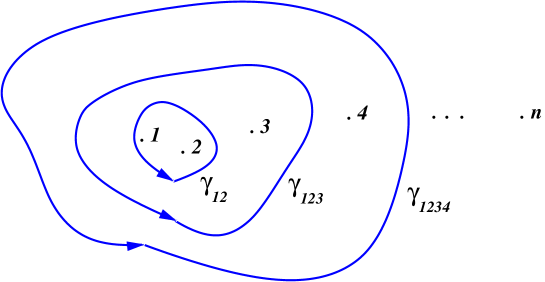
Figure 3: The elements $\gamma_{12},\ \gamma_{123},\ldots\gamma_{12...n-2}$ of the fundamental group ${\pi}_{1}(\mathbb{CP}^{1}\backslash\{z_{i}\})$. Choosing the accessory parameters in (2.1) according to (2.9) fixes the conjugacy classes of the associated elements of the monodromy group of (2.1) as given in (2.10).

The choice (2.9) of the accessory parameters in (2.1) fixes the conjugacy classes

$${\rm Tr}(M_{12})=-2\,\cos(\pi\nu_{1}),\ {\rm Tr}(M_{123})=-2\,\cos(\pi\nu_{2}),\ \ldots\ {\rm Tr}(M_{12\ldots n-2})=-2\,\cos(\pi\nu_{n-3})\,.$$ (2.10)

A neat geometric way to express the above statement is as follows [17]. The $n-3$ monodromy parameters $\nu_{1},\ldots\nu_{n-3}$ can be taken as a half of local coordinates on the moduli space of flat connections. It is easy to see that these variables are Poisson-commuting with respect to the Atiyah-Bott symplectic form.

One can then define, using a geometric construction involving an $n$-gon in the group $\mathbb{SL}(2,{\mathbb{C}})$ [17], a set of canonically conjugate variables ${\mu}_{1},\ldots{\mu}_{n-3}$, so that

$$\Omega=\sum_{i=1}^{n-3}\,{\rm d}\nu_{i}\wedge{\rm d}\mu_{i}\ .$$ (2.11)

In view of (2.9), it is useful to introduce a function (1.7), with an appropriate choice of the term $W_{0}(\boldsymbol{\nu})$. This function then generates the canonical transformation between the coordinates $(c_{i},z_{i})$ to another set of local coordinates $(\nu_{i},\mu_{i})$,

$$\mu_{i}=\frac{\partial W}{\partial\nu_{i}}\,,\qquad c_{i}=\frac{\partial W}{\partial z_{i}}\ .$$ (2.12)

In the simplest nontrivial case $n=4$ Eq.(2.1) is known as the Heun equation,

$$\psi^{\prime\prime}(z)+\left(\,\frac{\delta_{1}}{z^{2}}+\frac{\delta_{2}}{(z-x)^{2}}+\frac{\delta_{3}}{(z-1)^{2}}+\frac{x(x-1)\,C}{z(z-1)(z-x)}-\frac{\delta_{1}+\delta_{2}+\delta_{3}-\delta_{4}}{z(z-1)}\,\right)\psi(z)=0\,.$$ (2.13)

The four-point classical conformal block $f_{\nu}(x)$ solves the monodromy problem for this equation in the following sense. The choice

$$C=C(x,\nu)=\frac{\partial}{\partial x}\,f_{\nu}(x)$$ (2.14)

of the accessory parameter $C$ in (2.13) fixes the conjugacy class of the monodromy along the path $\gamma_{12}=\gamma_{1}\circ\gamma_{2}$ (see Fig. 4),

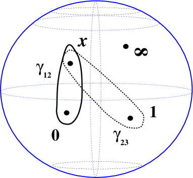
Figure 4: Elements $\gamma_{12}=\gamma_{1}\circ\gamma_{2}$ and $\gamma_{23}=\gamma_{2}\circ\gamma_{3}$ of the fundamental group of $\mathbb{CP}^{1}$ with four punctures. The parameters $\nu,\ \mu$ describe the conjugacy classes of $M(\gamma_{12})$ and $M(\gamma_{23})$ via Eqs.(2.15), (2).

$${\rm Tr}\big{(}M(\gamma_{12})\big{)}=-2\,\cos(\pi\nu)\,.$$ (2.15)

On the other hand

$${\mu}=\frac{\partial}{\partial\nu}\,\big{(}W_{0}({\nu})+f_{\nu}(x)\big{)}$$ (2.16)

determines the conjugacy class of the monodromy along the path $\gamma_{23}=\gamma_{2}\circ\gamma_{3}$ (see Fig. 4). With the choice

$$W_{0}(\nu)=-\frac{1}{4}\ \int{\rm d}\nu\ \log\big{(}\,\Omega(\nu,\lambda_{1}+\lambda_{2})\,\Omega(\nu,\lambda_{1}-\lambda_{2})\,\Omega(\nu,\lambda_{3}+\lambda_{4})\,\Omega(\nu,\lambda_{3}-\lambda_{4})\,\big{)}\ ,$$ (2.17)

where

$$\Omega(\nu,\lambda)=\frac{\Gamma(\frac{1}{2}+\frac{\nu}{2}+\frac{\lambda}{2})\,\Gamma(\frac{1}{2}+\frac{\nu}{2}-\frac{\lambda}{2})}{\Gamma(\frac{1}{2}-\frac{\nu}{2}+\frac{\lambda}{2})\,\Gamma(\frac{1}{2}-\frac{\nu}{2}-\frac{\lambda}{2})}\ \frac{\Gamma(1-\nu)}{\Gamma(1+\nu)}\ ,$$

this relation reads, explicitly (cf. [17]):

$${\rm Tr}\big{(}M(\gamma_{23})\big{)} = -\frac{\cosh(2\mu)}{2\,{\sin}^{2}({\pi}{\nu})}\ \sqrt{c_{12}({\nu})c_{34}({\nu})}$$

$$- \frac{(m_{1}-m_{2})(m_{3}-m_{4})}{8\,{\cos}^{2}(\frac{\pi\nu}{2})}+\frac{(m_{1}+m_{2})(m_{3}+m_{4})}{8\,{\sin}^{2}(\frac{\pi\nu}{2})}\ ,$$

where $m_{i}$’s were defined in (2.4) and

$$c_{ij}({\nu})=16\,{\cos}\big{(}{\textstyle\frac{\pi}{2}}({\nu}+{\lambda}_{i}+{\lambda}_{j})\big{)}\,{\cos}\big{(}{\textstyle\frac{\pi}{2}}({\nu}+{\lambda}_{i}-{\lambda}_{j})\big{)}\,{\cos}\big{(}{\textstyle\frac{\pi}{2}}({\nu}-{\lambda}_{i}+{\lambda}_{j})\big{)}\,{\cos}\big{(}{\textstyle\frac{\pi}{2}}({\nu}-{\lambda}_{i}-{\lambda}_{j})\big{)}\ .$$ (2.19)

3 Hamilton-Jacobi equation and Painlevé VI

3.1 Classical limit of $V_{(2,1)}$

The equation (2.1) has emerged in the classical limit from the insertion of the degenerate vertex operator $V_{(1,2)}$. Inserting the other level-2 degenerate operator $V_{(2,1)}$ has quite different effect. In the limit $b\to 0$ its dimension $\Delta_{(2,1)}$ goes to infinity as $-3/4b^{2}$, therefore the $n+1\,-\,$point conformal block with the $V_{(2,1)}$ insertion exponentiates as

$$\langle\,V_{(2,1)}(y)V_{\Delta_{1}}(z_{1})\ldots V_{\Delta_{n}}(z_{n})\,\rangle_{b\to 0}\sim\exp\big{(}\,{\textstyle\frac{1}{b^{2}}}\,S(y,\{z_{i}\})\,\big{)}\,.$$ (3.1)

The null-vector decoupling equation has the form (2.7) but with $b$ replaced with $b^{-1}$, so that the coefficient in front of the second derivative becomes large. This is fully consistent with the WKB form (3.1), and leads to the Hamilton-Jacobi - like equation (see e.g. [21])

$$\left(\frac{\partial S}{\partial y}\right)^{2}+\sum_{i=1}^{n}\,\left(\,\frac{\delta_{i}}{(y-z_{i})^{2}}+\frac{1}{y-z_{i}}\,\frac{\partial S}{\partial z_{i}}\,\right)=0\ .$$ (3.2)

Here we will show how this equation can be quite useful in the simplest nontrivial case of $n=4$. Thus, we will start with the 5-point conformal block with one of its insertions being $V_{(2,1)}(y)$. We use projective transformations to move $z_{1}$, $z_{3}$, and $z_{4}$ to the positions $0$, $1$ and $\infty$, respectively, and we denote $z_{2}=t$. In the classical limit we have

$$\langle\,V_{(2,1)}(y)V_{\Delta_{1}}(0)V_{\Delta_{2}}(t)V_{\Delta_{3}}(1)V_{\Delta_{5}}(\infty)\,\rangle_{b\to 0}\ \sim\ \exp\big{(}\,{\textstyle\frac{1}{b^{2}}}\,{S}(y,t)\,\big{)}\,.$$ (3.3)

At this point we do not specify the particular choice of the conformal block. Note also that we denoted $\Delta_{5}$, not $\Delta_{4}$, the dimension associated with $z_{4}=\infty$; the reason will become clear soon. Introducing the function

$$\tilde{S}(y,t)={S}(y,t)+\varphi(y,t)\,,$$ (3.4)

$$\varphi(y,t)=\big{(}\delta_{1}+\delta_{2}-{\textstyle\frac{1}{4}}\big{)}\,\log(t)+\big{(}{\textstyle\frac{1}{4}}+\delta_{2}+\delta_{3}-\delta_{1}-\delta_{5}\big{)}\log(1-t)-{\textstyle\frac{1}{2}}\,\log\big{(}y(y-1)\big{)}$$

allows one write the equation (3.2) as the conventional Hamilton-Jacobi equation

$$\frac{\partial{\tilde{S}}}{\partial t}+H\left(y,\frac{\partial{\tilde{S}}}{\partial y},t\right)=0$$ (3.5)

for a one-dimensional dynamical system with the phase-space coordinates $(y,p)$ and the time-dependent Hamiltonian

$$H(y,p,t)=\frac{(y-t)y(1-y)}{t(1-t)}\ p^{2}-\frac{\delta_{1}-\frac{1}{4}}{y(1-t)}-\frac{\delta_{2}}{t-y}-\frac{y(\delta_{3}-\frac{1}{4})}{t(y-1)}-\frac{(\delta_{5}-\frac{1}{4})\,y}{t(1-t)}\ .$$ (3.6)

Here, as before, $\delta_{i}$ are classical dimensions associated with $\Delta_{i}$ in (3.3).

3.2 Painlevé VI

The Hamiltonian might not look terribly attractive, but the corresponding equation of motion

$${\ddot{y}} = \frac{1}{2}\,\Big{(}\frac{1}{y}+\frac{1}{y-1}+\frac{1}{y-t}\Big{)}\,{\dot{y}}^{2}-\Big{(}\frac{1}{t}+\frac{1}{t-1}+\frac{1}{y-t}\Big{)}\ {\dot{y}}$$

$$+ \frac{2y(y-1)(y-t)}{t^{2}(1-t)^{2}}\ \bigg{(}\,\big{(}\delta_{1}-{\textstyle\frac{1}{4}}\big{)}\,\frac{t}{y^{2}}+\delta_{2}\,\frac{t(t-1)}{(y-t)^{2}}+\big{(}\delta_{3}-{\textstyle\frac{1}{4}}\big{)}\,\frac{1-t}{(y-1)^{2}}+{\textstyle\frac{1}{4}}-\delta_{5}\,\bigg{)}$$

is recognized as the celebrated Painlevé VI equation. This is of course the most general of the ordinary differential equations of the type ${\ddot{y}}=R(y,{\dot{y}},t)$ whose solutions $y(t)$ have no “movable singularities” but simple poles. Movable singularities are the singularities of a solution $y(t)$, viewed as the function of complex $t$, whose locations depend on the specific choice of the solution. Since by construction it is natural to regard the variable $y$ as living on the Riemann sphere, the simple poles are not really singularities, and one can say that the solutions of (3.2) have no movable singularities at all. Of course, there are “fixed” singularities of the solutions $y(t)$ at $t=0,1,\infty$.

3.3 Classical conformal block as Painlevé VI action

How this relation to the Painlevé VI can be useful in evaluating the classical conformal block in Fig. 5?

\psfrag{z1}{\large{$0,\delta_{1}$}}\psfrag{z2}{\large{$x,\delta_{2}$}}\psfrag{z3}{\large{$\delta_{\nu}$}}\psfrag{z4}{\large{$1,\delta_{3}$}}\psfrag{z5}{\large{$\infty,\delta_{4}$}}\includegraphics[width=284.52756pt]{4block_a.eps}

Figure 5: Dual diagram representing the classical conformal block $f_{\nu}(x)$.

Let us first make the following trivial observation. Let $y(t)$ be a solution of (3.2) such that

$$y(t_{1})=y_{1}\,,\qquad y(t_{2})=y_{2}\,.$$ (3.8)

Then by the definition of the classical action we have

$$\langle\,V_{(2,1)}(y_{2})\,V_{\Delta_{1}}(0)\,V_{\Delta_{2}}(t_{2})\,V_{\Delta_{3}}(1)\,V_{\Delta_{5}}(\infty)\,\rangle_{b\to 0}\ \sim\ \exp\Big{[}\,{\textstyle\frac{1}{b^{2}}}\,\big{(}\,\varphi(y_{1},t_{1})-\varphi(y_{2},t_{2})\,\big{)}\,\Big{]}\times$$

$$\ \ \ \ \exp\left(\,{\frac{1}{b^{2}}}\,\int_{t_{1}}^{t_{2}}{\rm d}t\ L(y,{\dot{y}},t)\,\right)\ \ \ \langle\,V_{(2,1)}(y_{1})\,V_{\Delta_{1}}(0)\,V_{\Delta_{2}}(t_{1})\,V_{\Delta_{3}}(1)\,V_{\Delta_{5}}(\infty)\,\rangle_{b\to 0}\ ,$$ (3.9)

where $\varphi(y,t)$ is the same as in (3.4), and $L(y,{\dot{y}},t)$ is the Lagrangian associated with the Hamiltonian (3.6). As was mentioned, general solution $y(t)$ is singular at $t=0,1,\infty$. Choose one of these points, say $t=0$. Near this singularity $y(t)$ behaves as $y(t)\to-\kappa\,t^{\nu}$ where $\kappa$ and $\nu$ are parameters of the solution. The exponent $\nu$ always satisfies $0\leq\Re\,\nu\leq 1$, so that generally $y(t)\to 0$ as $t\to 0$. Therefore, if one chooses $t_{1}=0$ in (3.9), three of the five points in the conformal block in the r.h.s. collide, and thus it reduces to a constant. On the other hand, the same trajectory $y(t)$ passes, at some nonsingular values of $t=x\neq 0,1,\infty$, through the other insertion points $0$, $t$, $1$, or $\infty$. At any such event two of the five insertions in the l.h.s. five-point conformal block in (3.9) merge, and it becomes a four point block. Thus such trajectory $y(t)$ interpolates between the three-point block (a constant) and a four point block which, according to (3.9) is then expressed essentially through the action $\int_{0}^{x}{\rm d}t\,L(y,{\dot{y}},t)$ evaluated on the trajectory. This outlines our strategy.

Let us add some details. For a solution $y(t)$ we call the “intercept points” the (generally complex) values of $t\neq 0,1,\infty$ at which $y(t)$ takes any of the values $y(t)=0,t,1,\infty$. Note that according to the Painlevé property (no movable singularities) the intercept points are regular point of $y(t)$ on the Riemann sphere. Out strategy requires setting $t_{2}$ in (3.9) equal to one of the intercept points. For definiteness, assume that the intercept point closest to zero is a pole at some $t=x$. The equation (3.2) dictates two possibilities for the residue at the pole, $y(t)\to\pm\,\frac{1}{\lambda_{5}}\,\frac{x(1-x)}{t-x}$ as $t\to x$, where $\lambda_{5}$ parameterizes the classical dimension $\delta_{5}=\frac{1-\lambda_{5}^{2}}{4}$. As explained above, at $t_{2}=x$ the l.h.s. of (3.9) becomes the four point conformal block

$$\langle\,V_{\Delta_{1}}(0)\,V_{\Delta_{2}}(x)\,V_{\Delta_{3}}(1)\,V_{\Delta_{4}}(\infty)\,\rangle_{b\to 0}\ .$$ (3.10)

Here $\Delta_{4}$ is related to $\Delta_{5}$ in (3.9) through the well known fusion rule [1]

$$V_{(2,1)}V_{\Delta(P)}=\big{[}\,V_{\Delta(P+{\rm i}/2b)}\,\big{]}+\big{[}\,V_{\Delta(P-{\rm i}/2b)}\,\big{]}\ .$$ (3.11)

The fusion rule (3.11) suggests two possible values for the classical dimension $\delta_{4}$ associated with $\Delta_{4}$ in (3.10), namely $\delta_{4}=\frac{1-(\lambda_{5}\pm 1)^{2}}{4}$. In fact, in the classical limit only one of the two terms in (3.11) dominates. It turns out that at all $\lambda_{5}$ with non-negative real part the dominating term corresponds to $\lambda_{4}=\lambda_{5}+1$, at least for $x$ sufficiently close to $0$ (we have verified this statement numerically for real $\lambda_{4}$), so that we have to take $\delta_{5}=\frac{1-(\lambda_{4}-1)^{2}}{4}$ in order to reproduce given $\delta_{4}=\frac{1-\lambda_{4}^{2}}{4}$.

To summarize, in evaluating the classical conformal block emerging in the limit $b\to 0$ of (3.10), we are interested in the solution of the Painlevé VI equation (3.2) with the following properties

$$y(t)\to-\kappa\,t^{\nu}\qquad\qquad\qquad\qquad\ \ \ \ \ \ \ \ \ \text{as}\quad t\to 0\,,$$ (3.12)

$$y(t)=\frac{1}{\lambda_{4}-1}\,\frac{x(1-x)}{t-x}+y_{0}+\ldots\qquad\text{as}\quad t\to x\,,$$ (3.13)

where the dots in the second line represent a power series in $(t-x)$. In (3.12) $\nu$ and $x$ should be regarded as independent parameters; equation (3.2) then determines $\kappa$ and $y_{0}$ as the functions of these. Note that in (3.13) we have chosen one of two signs of the residue at $t=x$ consistent with (3.2); this choice leads to the desired value $\frac{1-\lambda_{4}^{2}}{4}$ for the classical dimension $\delta_{4}$, while the opposite sign of the residue would produce $\frac{1-(2-\lambda_{4})^{2}}{4}$. Once the solution is found, the classical conformal block is expressed through the Painlevé VI action evaluated on this solution, from $t=0$ to $t=x$, according to the Eq.(3.9).

3.4 Regularized action and accessory parameter

Although the solution $y(t)$ described in the previous subsection is singular only at the singular points $0,1,\infty$, the Lagrangian $L(y,{\dot{y}},t)$ has poles at all intercept points. In particular, the action integral in (3.9), when specified to $t_{1}=0$ and $t_{2}=x$, diverges logarithmically at both ends of the integration contour. These divergences are well expected. Thus, the divergence at $t\to x$ reproduces the classical limit of the divergence of the operator product expansion

$$V_{(2,1)}(y(t))V_{\Delta_{5}}(\infty)\ \sim\ (y(t))^{\Delta_{4}-\Delta_{5}-\Delta_{(2,1)}}\,V_{\Delta_{4}}(\infty)\qquad\text{as}\quad y(t)\to\infty$$ (3.14)

in (3.9), while the divergence at $t\to 0$ represents the singular fusion of the three chiral vertices $V_{(2,1)}(y(t))V_{\Delta_{1}}(0)V_{\Delta_{2}}(t)$.

This interpretation leads to the regularization prescription. One adds $x$-independent counterterms to the classical action designed to compensate for the divergences of the OPE coefficients. The result is the the following regularized expression for the classical conformal block

$$f_{\nu}(x) = (\delta_{\nu}-\delta_{1}-\delta_{2})\ \log(x)+(\delta_{1}-\delta_{2}-\delta_{3}+\delta_{4})\ \log(1-x)$$

$$+ \frac{\nu}{2}\ \Big{(}\log\big{(}\kappa/\kappa_{0}\big{)}+\nu\,\log(x)\,\Big{)}+\int_{0}^{x}\,dt\,\bigg{(}\,L(y,{\dot{y}},t)-\frac{\nu^{2}}{4t}-\frac{\lambda_{4}-1}{2(x-t)}\,\bigg{)}\ ,$$

where $\delta_{i}={\textstyle\frac{1}{4}}\ (1-\lambda_{i}^{2})$ and

$$\kappa_{0}=\lim_{x\to 0}\big{(}x^{\nu}\,\kappa(x,\nu)\big{)}=\frac{4\,\nu^{2}}{(\nu-1-\lambda_{3}+\lambda_{4})(\nu-1+\lambda_{3}+\lambda_{4})}$$ (3.16)

is fixed by the condition (1.8) (see Eqs. (3.20), (3.21) and (3.22) below).

This formula looks somewhat difficult for practical applications. However, if one is interested in the accessory parameter (2.14), it is possible to bypass altogether the evaluation of the action integral in (3.4). Indeed, the derivative of the action with respect to $x$ generates two terms. The first, easy term comes from the upper integration limit, while the second, more difficult terms accounts for the derivative of the solution $y(t)$ itself with respect to $x$. But since the action is stationary with respect to the variations around the trajectory $y(t)$, this second term reduces to the boundary contribution. As the result, one finds

$$C(x,\nu)=\frac{\partial f_{\nu}(x)}{\partial x}=\frac{(\lambda_{4}-1)^{2}}{x(1-x)}\ (x-y_{0})+\frac{\delta_{3}-\delta_{1}+\delta_{2}-\delta_{4}}{x}+\frac{\delta_{2}+\delta_{3}+\delta_{4}-\delta_{1}}{1-x}\ ,$$ (3.17)

where $y_{0}=y_{0}(x,\nu)$ is the constant term in the expansion (3.13). Thus, finding the accessory parameter $C(x,\nu)$ is closely related to solving the connection problem for the Painlevé VI equation, i.e. relating the parameters $(x,y_{0})$ to $(\nu,\kappa)$. Similar calculation yields

$$\frac{\partial f_{\nu}(x)}{\partial\nu}=\frac{1}{2}\ \log(\kappa)-\frac{1}{2}\ \frac{\partial}{\partial\nu}\,\big{(}\nu\,\log(\kappa_{0})\big{)}\ .$$ (3.18)

We note that Eqs.(3.17), (3.18) generalize the equations (4.36) of Ref.[22] obtained previously for the monodromy of the Mathieu equation and connection problem of Painlevé III.

3.5 Power series

As is well known (see e.g.[23]), in the vicinity of the singular point, e.g. near $t=0$, the solution $y(t)$ with the asymptotic behavior (3.12) expands in a double power series

$$\frac{1}{y(t)}=\sum_{n=0}^{\infty}t^{n}\ U_{n}(t)\,,\qquad U_{n}(t)=\sum_{m=-n-1}^{n+1}t^{-\nu m}\ U_{n,m}\,,$$ (3.19)

where all the coefficients $U_{n,m}$ are uniquely determined by the equation (3.2) once the parameters $\nu$ and $\kappa$ are given. In particular

$$U_{0}(t) = -\frac{(\nu+\lambda_{3}-\lambda_{5})(\nu-\lambda_{3}-\lambda_{5})}{4\,\nu^{2}}\,A\ t^{\nu}-\frac{(\nu-\lambda_{3}+\lambda_{5})(\nu+\lambda_{3}+\lambda_{5})}{4\,\nu^{2}}\,A^{-1}\ t^{-\nu}$$ (3.20)

$$+ \frac{\nu^{2}-\lambda_{3}^{2}+\lambda_{5}^{2}}{2\,\nu^{2}}\ .$$

where $\lambda_{5}=\lambda_{4}-1$ and $A$ relates to $\kappa$ as

$$A=\frac{(\nu-\lambda_{3}+\lambda_{5})(\nu+\lambda_{3}+\lambda_{5})}{4\,\nu^{2}}\ \kappa\ .$$ (3.21)

The expansion (3.19) allows one to develop expansion of the accessory parameter (2.14) in power series of $x$ as follows. For small $x$, we are interested in the solution $y(t)$ satisfying (3.12) with $\kappa\gg 1$; if this condition is met, $y(t)$ develops poles at sufficiently small values of $t$, where $1/y(t)$ is still dominated by the low-$n$ terms of the expansion (3.19). Let us make technical assumption that $\Re e(\nu)$ is small (in fact we only need $\Re e(\nu)<1$), so that the term $U_{0}(t)$ in (3.19) dominates at small $t$. Neglecting all terms with $n>0$ leads to quadratic equation which determines points $t=x$, $|x|\ll 1$ such that $1/y(x)=0$. The roots of this equation

$$x^{\nu}=A^{-1}\qquad\text{and}\qquad x^{\nu}=A^{-1}\ \frac{(\nu-\lambda_{3}+\lambda_{5})(\nu+\lambda_{3}+\lambda_{5})}{(\nu+\lambda_{3}-\lambda_{5})(\nu-\lambda_{3}-\lambda_{5})}$$ (3.22)

provide potential initial approximation for the position of the pole $t=x$ in (3.12). It is not difficult to check that only the first of these roots corresponds to the correct sign of the residue at the pole, as show in (3.12); the second root would lead to the opposite sign, and thus to the wrong value $\frac{1-(2-\lambda_{4})^{2}}{4}$ instead of $\frac{1-\lambda_{4}^{2}}{4}$ of the classical dimension $\delta_{4}$. With this choice, one can systematically take into account the higher-$n$ terms in the expansion (3.19), which leads to the power-like corrections to the equation determining the pole position $x$ in terms of $\nu$ and $\kappa$,

$$A\,x^{\nu}=1+a_{1}\,x+a_{2}\,x^{2}+\ldots\ ,$$ (3.23)

where $A$ is given by (3.21), and the coefficients $a_{k}$ are systematically computed order by order in terms of $A$ and $\nu$, for example,

$$a_{1}=-\frac{\nu}{2}\ \bigg{(}1+\frac{16\,(\delta_{1}-\delta_{2})(\delta_{3}-\delta_{4})}{(1-\nu^{2})^{2}}\,\bigg{)}\ .$$ (3.24)

Expressions for the higher coefficients quickly become rather cumbersome, and we do not present them here. Finally, according to (3.17), the accessory parameter $C(x,\nu)$ can be expressed through the slope and the curvature of the function $U(t)=1/y(t)$ at its zero $t=x$,

$$C=\frac{1}{2}\,x(1-x)\,\Big{[}\,U^{\prime\prime}(t)+2t\,\big{(}U^{\prime}(t)\big{)}^{2}\Big{]}_{t=x}+\frac{\delta_{3}-\delta_{1}+\delta_{2}-\delta_{4}}{x}+\frac{\delta_{2}+\delta_{3}+\delta_{4}-\delta_{1}}{1-x}\ .$$ (3.25)

Explicit calculation yields

$$C = \frac{\delta_{\nu}-\delta_{1}-\delta_{2}}{x}+\frac{(\delta_{\nu}-\delta_{1}+\delta_{2})(\delta_{\nu}-\delta_{4}+\delta_{3})}{2\,\delta_{\nu}}+\bigg{(}\,\frac{(\delta_{\nu}-\delta_{1}+\delta_{2})(\delta_{\nu}-\delta_{4}+\delta_{3})}{2\,\delta_{\nu}}$$

$$+ \frac{\big{(}\,\delta_{\nu}^{2}+2\,\delta_{\nu}\,(\delta_{1}+\delta_{2})-3\,(\delta_{1}-\delta_{2})^{2}\,\big{)}\big{(}\,\delta^{2}_{\nu}+2\,\delta_{\nu}\,(\delta_{3}+\delta_{4})-3\,(\delta_{3}-\delta_{4})^{2}\,\big{)}}{32\,\delta^{2}_{\nu}\,(\delta_{\nu}+\frac{3}{4})}$$

$$- \frac{\big{(}\,(\delta_{1}-\delta_{2})^{2}-\delta^{2}_{\nu}\,\big{)}\big{(}\,(\delta_{3}-\delta_{4})^{2}-\delta^{2}_{\nu}\,\big{)}}{8\,\delta_{\nu}^{3}}\,\bigg{)}\ x+O(x^{2})\ ,$$

in complete agreement with the classical limit of well known expansion coefficients of the four point conformal block.

4 Remarks

It is well known that the Painlevé VI equation describes the isomonodromic deformations of the second order Fuchsian system with four singular points. Consider the linear problem

$$\partial_{z}{\boldsymbol{\Psi}}(z)={\boldsymbol{A}}(z)\,{\boldsymbol{\Psi}(z)}\,,\qquad{\boldsymbol{A}}(z)=\frac{{\boldsymbol{A}}_{1}}{z}+\frac{{\boldsymbol{A}}_{2}}{z-t}+\frac{{\boldsymbol{A}}_{3}}{z-1}\ ,$$ (4.1)

where ${\boldsymbol{A}}_{i}$ are constant (i.e. $z$-independent) traceless $2\times 2$ matrices with ${\rm det}({\boldsymbol{A}}_{i})=-\frac{\lambda_{i}^{2}}{4}$, and ${\boldsymbol{\Psi}}=\left(\begin{array}[c]{cc}\psi_{+}&\\ \psi_{-}&\end{array}\!\!\!\!\!\!\right)$. If ${\boldsymbol{A}}_{4}=-\sum_{i=1}^{3}{\boldsymbol{A}}_{i}\neq 0$ then there are four regular singularities $t$, $0$, $1$ and $\infty$. It is convenient to choose the gauge such that ${\boldsymbol{A}}_{4}={\rm diag}(\lambda_{4}/2,-\lambda_{4}/2)$, so that the off-diagonal elements of the matrix ${\boldsymbol{A}}(z)$ in (4.1) decay as $1/z^{2}$ as $z\to\infty$. Define $y$ as the zero of the off-diagonal matrix element $B(z)$ of the matrix

$${\boldsymbol{A}}(z)=\left(\begin{array}[c]{cc}A(z)&\ \ \,B(z)\\ C(z)&-A(z)\end{array}\right)$$ (4.4)

in (4.1), which then must have the form

$$B(z)=k\ \frac{y-z}{z(z-1)(z-t)}\,.$$ (4.5)

The parameter $k$ can be set to $1$ by the remaining gauge transformation.

The linear Fuchsian systems admit monodromy preserving deformations, generally expressed by the Schlesinger’s equations [24, 25]. For the system (4.1), these equations reduce to the Painlevé VI equation (3.2) for the parameter $y$ as the function of $t$ (with the equations for the remaining elements of the matrices ${\boldsymbol{A}}_{i}$ dependent of this function).

The Darboux coordinates $({\nu},{\mu})$ of the $\mathbb{SL}(2,\mathbb{C})$ flat connection ${\boldsymbol{A}}(z)$ defined in [17] can be computed at any point of the Schlesinger-Painlevé VI flow, in particular in the limit $t\to 0$. In this limit the connection (4.1) reduces to a pair of hypergeometric connections on the $3$-punctured spheres, connected by certain gauge transformation, and can be evaluated in closed form. Thus, the coordinate ${\nu}$ is determined in this limit from the eigenvalues of ${\boldsymbol{A}}_{1}+{\boldsymbol{A}}_{2}$, confirming that it coincides with the parameter $\nu$ in (3.12). Similarly, calculating the connection at $t\to 0$ allows one to relate the coordinate $\mu$ to the parameter $\kappa$ in (3.12), in full agreement with (2.16), (3.18). We note that this agreement can be regarded as an alternative derivation of (3.4) which, unlike our arguments in Section 3, avoids any references to quantum conformal blocks. However, we believe that the arguments in Section 3 are more compact and suggestive.

The $n>4$ generalization of our formalism seems to be straightforward. Let ${\mathcal{A}}_{0,n}$ be the moduli space of representations of the fundamental group of the $n$-punctured sphere into $\mathbb{SL}(2,\mathbb{C})$ with the fixed conjugacy classes of the elementary loops. It is endowed with the symplectic form $\Omega$ whose Darboux coordinates $({\nu}_{i},{\mu}_{i})$, $i=1,\ldots n-3$, are defined in [17] relative to a pant decomposition of the $n$-punctured sphere. On the other hand, the space ${\mathcal{X}}_{n}$ of residues ${\boldsymbol{A}}_{i}$, $i=1,\ldots n$, with fixed eigenvalues ${\rm Tr}({\boldsymbol{A}}_{i}^{2})=\frac{1}{2}\,{\lambda}_{i}^{2}$, of the meromorphic ${\mathfrak{s}l}(2)$-connection

$${\boldsymbol{A}}(z)=\sum_{i=1}^{n}\frac{{\boldsymbol{A}}_{i}}{z-z_{i}}$$ (4.6)

obeying the moment map equation

$$\sum_{i=1}^{n}{\boldsymbol{A}}_{i}=0$$ (4.7)

and considered up to the simultaneous $\mathbb{SL}(2,\mathbb{C})$ conjugation, is a symplectic manifold, with the Darboux coordinates $(p_{i},y_{i}),\ i=1,\ldots n-3,$ defined relative to a point $(z_{1},\ldots z_{n})$ on the moduli space ${\mathcal{M}}_{0,n}$ of $n$-punctured sphere. Let us parameterize points of ${\mathcal{M}}_{0,n}$ by ${\bf z}=\{z_{1},\ldots z_{n-3}\}$, by setting $z_{n-2}=0$, $z_{n-1}=1$, $z_{n}=\infty$ (this is the same convention as we adopted in Sections 1 and 2 for generic $n$, but is slightly different from the conventions (1.3) chosen for $n=4$ in the main body of the paper). The coordinates $y_{i}$ are the zeros of the matrix element $B(z)$ defined in the general case in (4.4) in the gauge where ${\boldsymbol{A}}_{n}$ is diagonal. The coordinates $p_{i}$ are the eigenvalues of ${\boldsymbol{A}}(y_{i})$ (see [26, 27, 28, 29] for precise definitions). The map ${\Phi}:{\mathcal{M}}_{0,n}\times{\mathcal{X}}_{n}\longrightarrow{\mathcal{A}}_{0,n}$ sends the set of residues to the monodromy data of the connection (4.6). We have:

$${\Phi}^{*}{\Omega}=\sum_{i=1}^{n-3}{\rm d}p_{i}\wedge{\rm d}y_{i}-\sum_{i=1}^{n-3}{\rm d}h_{i}\wedge{\rm d}z_{i}\ ,$$ (4.8)

where $h_{i}({\bf p},{\bf y},{\bf z})$ are the Hamiltonians of the Schlesinger flows, generating the isomonodromic deformations of (4.6). Here and below ${\bf p}=\{p_{i}\}\,,\ {\bf y}=\{y_{i}\}$, etc. Writing the left hand side of (4.8) as ${\rm d}{\boldsymbol{\nu}}\wedge{\rm d}{\boldsymbol{\mu}}$ and taking the ${\rm d}$-antiderivative we arrive at the equation:

$${\rm d}S=\sum_{i=1}^{n-3}\left({\mu}_{i}\,{\rm d}{\nu}_{i}+p_{i}\,{\rm d}y_{i}-h_{i}\,{\rm d}z_{i}\right)$$ (4.9)

for some master function $S({\bf z},{\bf y},{\boldsymbol{\nu}})$, which solves the Hamilton-Jacobi equations

$$h_{i}\left(\frac{{\partial}S}{{\partial}{\bf y}},{\bf y},{\bf z}\right)=-\frac{{\partial}S}{{\partial}z_{i}}\,,\qquad i=1,\ldots n-3$$ (4.10)

and can be related in a standard way to the action evaluated on a solution of the Schlesinger equation. The function $S$ should be related to the $b\to 0$ limit of the $2n-3$-point conformal block

$$\Big{\langle}\,\prod_{i=1}^{n-3}V_{(2,1)}(y_{i})\prod_{i=1}^{n}V_{{\Delta}_{i}}(z_{i})\,\Big{\rangle}_{b\to 0}\ .$$ (4.11)

To make contact with the twisted superpotential $W({\boldsymbol{\nu}},{\bf q})$ of the linear quiver theory with the gauge group $\big{(}\mathbb{SU}(2)\big{)}^{\otimes(n-3)}$ in the context of the AGT correspondence, with the exponentiated complexified coupling $q_{i}$ of the $i^{\rm th}$ gauge factor given by $z_{i}/z_{i+1}$, proceed as follows. First pick a path ${\bf z}(t)$ in $\overline{{\mathcal{M}}_{0,n}}$ with $t\in\mathbb{CP}^{1}$, which originates at ${\bf z}(0)=0$ in such a way that $0<|\,z_{1}|\ll|\,z_{2}|\ll|\,z_{3}|\ll\ldots\ll|\,z_{n-3}|\ll 1$. This corresponds to the maximal degeneration of the $n$-punctured sphere at $t=0$, associated with the dual diagram in Fig. 1 (with the legs $1$ and $n-2$ interchanged). Also, let ${\bf z}={\bf z}(1)$. Now, consider a solution of Schlesinger equations restricted onto this path. The details of the path are not essential except for the global monodromy properties, because the Hamiltonians $h_{i}$ obey

$${\partial}_{z_{i}}h_{j}-{\partial}_{z_{j}}h_{i}=0\ ,\qquad\{h_{i},h_{j}\}_{\bf p,y}=0\ .$$ (4.12)

One must pick the solution such that for $t=1$ the corresponding zeroes $y_{i}$ are equal to the “moving points” $z_{i}$: $y_{i}({\bf z}(1))=z_{i}$. Then integrate $\int_{0}^{1}\,\left({\bf p}\,{\dot{\bf y}}-{\bf h}\,{\dot{\bf z}}\right)\,{\rm d}t$ and subtract the logarithmically divergent terms to arrive at $W({\boldsymbol{\nu}},{\bf z})$.

Potential developments of the relation discussed in this note include its extension to the general classical conformal blocks along the lines described above, in particular analysis of the suitable solutions of the Schlesinger equations, and its possible applications to the study of the analytic properties. We hope to come back to these problems in the future.

References

- [1] A. A. Belavin, A. M. Polyakov and A. B. Zamolodchikov, “Infinite conformal symmetry in two-dimensional Quantum Field Theory,” Nucl. Phys. B 241, 333 (1984).
- [2] N. Nekrasov, “On the BPS/CFT correspondence,” seminar at the string theory group, University of Amsterdam, Feb. 3, 2004.
- [3] N. A. Nekrasov, “Seiberg-Witten prepotential from instanton counting,” Adv. Theor. Math. Phys. 7, 831 (2004) [arXiv:hep-th/0206161].
- [4] A. S. Losev, A. Marshakov and N. A. Nekrasov, “Small instantons, little strings and free fermions,” In: Shifman, M. (ed.) et al.: From fields to strings, vol. 1, 581-621 [arXiv:hep-th/0302191].
- [5] N. Nekrasov and A. Okounkov, “Seiberg-Witten theory and random partitions” [arXiv:hep-th/0306238].
- [6] L. F. Alday, D. Gaiotto and Y. Tachikawa, “Liouville correlation functions from four-dimensional gauge theories,” Lett. Math. Phys. 91, 167 (2010) [arXiv:hep-th/0906.3219].
- [7] Al. B. Zamolodchikov, “Conformal symmetry in two-dimensions: recursion representation of conformal block,” Teor. Mat. Fiz. 73, No.1, 103 (1987) (Theor. Math. Phys., 53, 1088 (1987)).
- [8] A. B. Zamolodchikov and Al. B. Zamolodchikov, “Structure constants and conformal bootstrap in Liouville field theory,” Nucl. Phys. B 477, 577 (1996) [arXiv:hep-th/9506136].
- [9] O. Gamayun, N. Iorgov and O. Lisovyy, “Conformal field theory of Painlevé VI,” JHEP 1210, 038 (2012) [Erratum-ibid. 1210, 183 (2012)] [arXiv:hep-th/1207.0787].
- [10] Al. B. Zamolodchikov, “Conformal symmetry in two-dimensions: an explicit recurrence formula for the conformal partial wave amplitude,” Commun. Math. Phys. 96, 419 (1984).
- [11] V. A. Alba, V. A. Fateev, A. V. Litvinov and G. M. Tarnopolsky, “On combinatorial expansion of the conformal blocks arising from AGT conjecture,” Lett. Math. Phys. 98, 33 (2011) [arXiv:hep-th/1012.1312].
- [12] N. A. Nekrasov and S. L. Shatashvili, “Quantization of integrable systems and four dimensional gauge theories” [arXiv:hep-th/0908.4052].
- [13] N. Nekrasov, V. Pestun and S. Shatashvili, “Quantum geometry and quiver gauge theories,” to appear.
- [14] M. F. Atiyah and R. Bott, “The Yang-Mills equations over Riemann surfaces,” Phil. Trans. R. Soc. Lond. A 308, 523-615 (1982).
- [15] A. Bilal, V. V. Fock and I. I. Kogan, “On the origin of W algebras,” Nucl. Phys. B 359, 635 (1991).
- [16] P. Boalch, “Symplectic manifolds and isomonodromic deformations,” Adv. Math. 163, 137-205 (2001).
- [17] N. Nekrasov, A. Rosly and S. Shatashvili, “Darboux coordinates, Yang-Yang functional, and gauge theory,” Nucl. Phys. Proc. Suppl. 216, 69 (2011) [arXiv:hep-th/1103.3919].
- [18] L. Takhtajan and P. Zograf, “Action for the Liouville equation as a generating function for the accessory parameters and as a potential for the Weil-Petersson metric on the Teichmller space,” Funkts. Anal. Prilozh. 19, 67 (1985) [Engl. transl.: Funct. Anal. Appl. 19, 219 (1986)]; “On the Liouville equation, accessory parameters and the geometry of the Teichmller space for the Riemann surfaces of genus ,” Mat. Sbornik 132, 147 (1987) [Engl. transl.: Math. USSR Sbornik 60, 143 (1988)].
- [19] F. Klein, “Neue Beitrge zur Riemann’schen Functionentheorie,” Math. Ann. 21, 201 (1883).
-
[20]
A. Poincare,
“Sur les groupes des equations lineaires”, Acta Math., 4, 201 (1884);
“Les fonctions fuchsiennes et l’equation ,” J. Math. Pures Appl., 5, 157, (1898). - [21] J. Teschner, “Quantization of the Hitchin moduli spaces, Liouville theory, and the geometric Langlands correspondence I,” Adv. Theor. Math. Phys. 15, 471 (2011) [arXiv:hep-th/1005.2846].
- [22] S. L. Lukyanov, “Critical values of the Yang-Yang functional in the quantum sine-Gordon model,” Nucl.Phys. B 853, 475-507 (2011) [arXiv/hep-th:1105.2836].
- [23] D. Guzzetti, “Tabulation of PVI transcendents and parametrization formulas,” Nonlinearity 25, 3235 (2012) [arXiv:math.CA/1108.3401].
- [24] L. Schlesinger, “Ueber eine klasse von differentsial system beliebliger ordnung mit festen kritischer punkten”, J. fur Math. 141, 96 (1912).
- [25] M. Jimbo, T. Miwa and K. Ueno, “Monodromy preserving deformations of linear differential equations with rational coefficients (1),” Physica D 2, 407 (1981).
- [26] E. K. Sklyanin, “Goryachev-Chaplygin top and the inverse scattering method,” Zapiski Nauch. Semin. LOMI133, 236 257 (1984) [Engl. transl.: J. Soviet Math. 31, 3417 3431 (1985)];
- [27] E. K. Sklyanin, “Separation of variables – new trends,” Prog. Theor. Phys. Suppl. 118, 35-60 (1995) [arXiv:solv-int/9504001].
- [28] I. Krichever, “Isomonodromy equations on algebraic curves, canonical transformations and Whitham equations” [arXiv:hep-th/0112096].
- [29] B. Dubrovin, M. Mazzocco, “Canonical structure and symmetries of the Schlesinger equations” [arXiv:math/0311261].
- [30] A.-K. Kashani-Poor, J. Troost, “Transformations of spherical blocks” [arXiv:hep-th/1305.7408].