Steady self-diffusion in classical gases

Abstract

A steady self-diffusion process in a gas of hard spheres at equilibrium is analyzed. The system exhibits a constant gradient of labeled particles. Neither the concentration of these particles nor its gradient are assumed to be small. It is shown that the Boltzmann-Enskog kinetic equation has an exact solution describing the state. The hydrodynamic transport equation for the density of labeled particles is derived, with an explicit expression for the involved self-diffusion transport coefficient. Also an approximated expression for the one-particle distribution function is obtained. The system does not exhibit any kind of rheological effects. The theoretical predictions are compared with numerical simulations using the direct simulation Monte Carlo method and a quite good agreement is found.

1 Introduction

Self-diffusion is a particularly simple transport phenomenon in fluids that has attracted much attention [1, 2, 3, 4]. The situation usually considered corresponds to a very dilute concentration of tagged particles [1, 2, 3]. Moreover, the limit of small density gradient is considered. On the other hand, not too much attention has been devoted to study the peculiarities of self-diffusion as compared with mutual diffusion when the concentrations of the two components of the mixture are of the same order and the density gradients are large. Also the attention paid to states exhibiting a steady flux of tagged particles is rather restricted.

In this paper, self-diffusion will be understood as an idealization of a mutual two-component diffusion process in which the particles are all mechanically identical, but some of them are assumed to be distinguishable from the others, e.g., they carry a label, are colored, have some spin or are in different internal atomic state [5]. The system considered will be a gas at equilibrium. It is not assumed that the number of labeled particles is much smaller than the total number of particles, i.e. the density of both labeled and unlabeled particles can be of the same order. Moreover, the relative gradient of the density of labeled particles can be arbitrarily large.

It will be shown that the kinetic Boltzmann-Enskog equation has an exact solution describing the above state.The kinetic theory analysis is local and does not require specification of the boundary conditions of the distribution function necessary for the state.This is a relevant result since solutions of the Boltzmann-Enskog equation describing nontrivial non-equilibrium states are scarce, and they provide a solid starting point to develop a macroscopic theory of non-equilibrium states. Actually, the results are trivially extended to the Boltzmann equation for an arbitrary interaction potential.

2 The state and the kinetic equation

Consider a gas composed of mechanically identical particles of mass $m$ that is at equilibrium at temperature T, being $n$ the number of particles density. Then, the one-particle distribution function $f({\bm{v}})$ of the system has the form

$$f({\bm{v}})=n\varphi(v),$$ (1)

where $\varphi(v)$ is the Maxwellian velocity distribution,

$$\varphi(v)=\left(\frac{m}{2\pi k_{B}T}\right)^{d/2}e^{-\frac{mv^{2}}{2k_{B}T}}.$$ (2)

Here $d$ is the dimension ($2$ or $3$) of the system and $k_{B}$ is the Boltzmann constant. The above distribution refers to all particles without regards to the possible existence of labels. Suppose now that some of the particles are labeled, Their one-particle distribution function will be denoted by $f_{l}({\bm{r}},{\bm{v}},t)$. Since all the particles are mechanically equivalent, the equilibrium state of the system as a whole will be conserved in time, independently of the distribution of labeled particles.

The Enskog equation provides a successful empirical theory to study gases of hard particles beyond the limit of asymptotically small density, in which the Boltzmann equation applies [3, 4]. Moreover, the low density limit of any solution of the Enskog equation is a solution of the Boltzmann equation for hard spheres ($d=3$) or disks ($d=2$).

The state being analyzed here is characterized by a steady self-diffusion flow of labeled particles with gradients only in the $z$-direction. Applied to this state, the Enskog equation has the form

$$v_{z}\frac{\partial f_{l}(z,{\bm{v}})}{\partial z}=g_{e}(n)J_{B}[z,{\bm{v}}|f_{l},n\varphi],$$ (3)

where $g_{e}(n)$ is the equilibrium pair correlation function of two particles of the gas at contact and $J_{B}$ is the Boltzmann collision operator,

$$J_{B}[z,{\bm{v}}_{1}|f_{l},n\varphi] = n\sigma^{d-1}\int d{\bm{v}}_{2}\int d\widehat{\bm{\sigma}}\,\Theta\left({\bm{v}}_{12}\cdot\widehat{\bm{\sigma}}\right){\bm{v}}_{12}\cdot\widehat{\bm{\sigma}}$$

$$\times\left[f_{l}(z,{\bm{v}}_{1}^{\prime})\varphi(v^{\prime}_{2})-f_{l}(z,{\bm{v}}_{1})\varphi(v_{2})\right].$$

In this expression, $\sigma$ is the diameter of the particles, $d\widehat{\bm{\sigma}}$ is the solid angle element around the unit vector $\widehat{\bm{\sigma}}$ pointing from the center of particle $2$ to the center of particle $1$ at contact, ${\bm{v}}_{12}\equiv{\bm{v}}_{1}-{\bm{v}}_{2}$, and ${\bm{v}}_{1}^{\prime}$ and ${\bm{v}}_{2}^{\prime}$ are the precollisional velocities given by

$${\bm{v}}^{\prime}_{1}={\bm{v}}_{1}-{\bm{v}}_{12}\cdot\widehat{\bm{\sigma}}\widehat{\bm{\sigma}},\quad\quad{\bm{v}}^{\prime}_{2}={\bm{v}}_{2}+{\bm{v}}_{12}\cdot\widehat{\bm{\sigma}}\widehat{\bm{\sigma}}.$$ (5)

It is worth to mention that in the present context there is no difference between the original version of the Enskog equation [5] and the revised version introduced by van Beijeren and Ernst [6]. The reason is that the local density at which the equilibrium pair correlation must be evaluated is the total one, since this is the one determining the collision frequency, and this density is uniform. The validity of the linear Boltzmann equation obtained by putting $g_{e}=1$ in Eq. (3) to describe steady self-diffusion in the low density limit, has been discussed in detail in refs [7, 8]. Here, we will look for a normal solution to it having the form,

$$f_{l}(z,{\bm{v}})=n_{l}(z)\varphi(v)+\chi({\bm{v}})\varphi(v),$$ (6)

where the density profile $n_{l}$ defined by

$$n_{l}({\bm{r}},t)\equiv\int d{\bm{v}}\,f_{l}({\bm{r}},{\bm{v}},t),$$ (7)

is assumed to be linear,

$$n_{l}(z)=az+b,$$ (8)

$a$ and $b$ being constants to be fixed by the hydrodynamic boundary conditions. To guarantee that $n_{l}$ is the actual number density of labeled particles, the function $\chi$ introduced in Eq. (6) must verify

$$\int d{\bm{v}}\chi({\bm{v}})\varphi(v)=0.$$ (9)

Substitution of Eqs. (6) and (8) into Eq. (3) gives

$$v_{z}a\varphi(v)=g_{e}(n)J_{B}[{\bm{v}}|\chi\varphi,n\varphi],$$ (10)

where it has been taken into account that $\varphi$ is a steady solution of the Enskog equation, $J_{B}[{\bm{v}}|\varphi,\varphi]=0$. Eq. (10) verifies the solubility condition that the inhomogeneous term is orthogonal to the solutions of the homogeneous equation [4, 9], since the only collision invariant in this case is unity. Moreover, Eq. (9) establishes uniqueness of the solution. Because of the symmetry of the collision operator in Eq. (10), its solution has to be proportional to the scalar $av_{z}$, i.e.

$$\chi({\bm{v}})=av_{z}\psi(v),$$ (11)

where $\psi(v)$ is an isotropic function of the velocity. Then, the steady flux of labeled particles is given by

$$j_{l,z}\equiv\int d{\bm{v}}\,v_{z}f_{l}(z,{\bm{v}})=-Da,$$ (12)

with the self-diffusion coefficient identified as

$$D=-\int d{\bm{v}}v_{z}^{2}\psi(v)\varphi(v).$$ (13)

Substitution of Eq. (11) into Eq. (10) yields

$$v_{z}\varphi(v)=g_{e}(n)J_{B}[{\bm{v}}|v_{z}\psi\varphi,n\varphi].$$ (14)

Multiplication of this equation by $v_{z}$ and later integration over the velocity gives

$$D=\frac{k_{B}T}{mg_{e}n\nu_{D}},$$ (15)

where $\nu_{D}$ is a diffusive frequency given by

$$\nu_{D}=-\frac{\int d{\bm{v}}\,v_{z}J_{B}[{\bm{v}}|v_{z}\psi\varphi,\varphi]}{\int d{\bm{v}}\,v_{z}^{2}\psi(v)\varphi(v)}.$$ (16)

This expression agrees with the one obtained for the coefficient appearing in the self-diffusion equation to Navier-Stokes order, derived from the Enskog-Lorentz equation by means of the Chapman-Enskog procedure [4, 10]. It is worth to stress that in the present context, that equation is exact for the steady state under consideration. An explicit evaluation of the frequency $\nu_{D}$ requires some kind of approximation. In the first Sonine approximation, the function $\psi(v)$ becomes a constant, and it is obtained,

$$D=\frac{\Gamma(d/2)d}{4\pi^{(d-1)/2}n\sigma^{d-1}g_{e}(n)}\left(\frac{k_{B}T}{m}\right)^{1/2}.$$ (17)

Now, it is easy to compute the distribution function of labeled particles in the first Sonine approximation. Equations (6) and (11) lead to

$$f_{l}(z,v)=\left[n_{l}(z)-c_{D}av_{z}\right]\varphi(v),$$ (18)

The coefficient $c_{D}$ can be expressed in terms of the self-diffusion coefficient by use of Eq. (18) into Eq. (12), giving

$$f_{l}(z,{\bm{v}})=\left[n_{l}(z)-\frac{maDv_{z}}{k_{B}T}\right]\varphi(v).$$ (19)

Define velocity moments $\mu_{k}$ by

$$\mu_{k}\equiv\int d{\bm{v}}\,v_{z}^{k}f_{l}(z,{\bm{v}}),$$ (20)

$k=0,1,2,\ldots$ In particular, it is $\mu_{0}(z)\equiv n_{l}(z)$ and $\mu_{1}\equiv j_{l,z}\,$. From Eq. (19) it is obtained:

$$\mu_{k}(z)=c_{k}\mu_{0}(z),$$ (21)

for $k>0$ and even, and

$$\mu_{k}=-c_{k+1}\frac{amD}{k_{B}T},$$ (22)

for $k$ odd. Here,

$$c_{k}\equiv\left(\frac{2k_{B}T}{m}\right)^{k/2}\pi^{-1/2}\Gamma\left(\frac{k+1}{2}\right).$$ (23)

It must be noticed that Eq. (19) has been obtained considering the leading term in an expansion of the distribution function in orthogonal functions. The fact that it becomes negative for large values of $v_{z}$ is a consequence of this approximation.

3 Simulation results

To test the theoretical predictions presented above, computer simulations have been performed. In order to generate the steady self-diffusion state, the general approach initiated by Lees and Edwards [11] and Ashurst and Hoover [12] has been employed. The basic idea is to alter the boundary conditions in such a way that they drive the system into a non-equilibrium steady state. The specific boundaries used here for the self-diffusion problem are similar to those described by Erpenbeck and Wood in ref. [13].

The standard periodic boundary conditions are complemented by a color or label change algorithm, as described now. Whenever a particle leaves the system through the boundary located at $z=L$ ($z=0$) it is reinjected at $z=0$ ($z=L$), and it is labeled with probability $p$ ($q$), independently of whether it was or was not labeled before. Without loss of generality, the choice $q=1-p$ can be done in order to make symmetric the roles of labeled and unlabeled particles. The effect of the label change is to generate a difference in the number density of labeled particles at both boundaries. In the long time limit, it is expected that the system reaches a steady one-dimensional state with a uniform flux of labeled particles along the $z$ direction.

The main goal of the simulations to be presented is to verify the existence of the solution of the Boltzmann equation discussed above and to check the accuracy of the derived expressions. Note that if this solution exists, it is trivial that the corresponding solution of the Enskog equation also exists. For this reason, the simulation technique employed has been the direct simulation Monte Carlo (DSMC) method [14]. This is a particle simulation method designed to mimic the dynamics of a dilute gas of particles described by the Boltzmann equation. One advantage of the DSMC method is that it allows to explote the symmetry of the system. In the present case, we are interested in states showing gradients only in one direction. Consequently, it is enough to consider the system as limited by two infinite parallel walls located at z=0 and z=L, respectively, and to divide it into layers perpendicular to the $z$-axis, being irrelevant the coordinates of the particles perpendicular to the $z$-axis [14].

In the simulations, a gas of hard spheres ($d=3$) of diameter $\sigma$ has been employed. The reported results will be expressed in the units defined by the mass of the particles $m$, the average mean free path $\lambda=(\pi\sqrt{2}n\sigma^{2})^{-1}$, and the temperature $T$, taken such that $k_{B}T=1$. Although the number of particles $N$ used in the DSMC method does not affect the dynamics of the particles nor the physical density of the system, and it has only a statistical meaning, let us mention for the sake of completeness that in all the cases to be reported it has been $N/L=800\lambda^{-1}$.

The simulations started with the same number ($N/2$) of labeled and unlabeled particles uniformly distributed in the system. The initial velocity distribution of all particles was Gaussian with vanishing average. As expected, the system always reached a steady state, after some transient period. Once the system was in the steady state, the relevant quantities (hydrodynamic profiles, number of labeled particles flux, and velocity distribution) were measured. To identify the position dependence of the properties, the system was divided into layers of width $\Delta z=\lambda$. The results presented below have been averaged over a number of different trajectories, typically 200. Also, they have been time averaged over a period time of the order of 2000 collisions per particle.

A way of modifying the expected density gradient is to vary $p$ keeping constant the size of the system $L$. Another possibility is to keep constant the value of $p$ and to modify $L$. We have verified that both methods lead to equivalent results. Then, the choice has been made of taking $p=1$, so that the boundary conditions can be interpreted as the system being in contact with a reservoir of labeled particles at $z=L$ and a reservoir of unlabeled ones at $z=0$.

As an example, in Figs. 1 and 2 the number density and temperature profiles of labeled particles in a system with $L=60\lambda$ are plotted. The partial temperature of the labeled particles is defined by considering the peculiar velocities with respect to the whole gas, which is at rest. This explains the abrupt variation of the partial temperature near the boundary at $z=0$. The flux of labeled particles for the same system is given in Fig. 3. Its profile is uniform as it must be in a steady state, and no significant boundary layer is identified. Similar results were obtained in systems with $L=30\lambda$ and $L=90\lambda$.

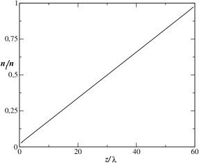
Figure 1: Steady relative number density profile of labeled particles for a system of hard spheres of width $L=60\lambda$, where $\lambda$ is the mean free path of the gas.

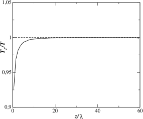
Figure 2: Steady temperature profile of labeled particles $T_{l}$ for a system of hard spheres of width $L=60\lambda$, where $\lambda$ is the mean free path of the gas. The temperature is scaled with the temperature of the system $T$.

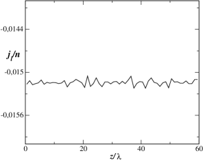
Figure 3: Steady flux of labeled particles $j_{l,z}$ profile for a system of hard spheres of width $L=60\lambda$, where $\lambda$ is the mean free path of the gas. The flux is measured in the dimensionless units defined in the main text.

The linearity of the density profiles indicates the absence of linear rheological effects that would affect the shape of the density profile. By fitting the profiles to a straight line, the values $a$ of the slope have been measured. This quantity differs from $1/L$ due to the existence of kinetic boundary layers near both walls. Then, from the values of the current $j_{l,z}$ and $a$, the self-diffusion constant was obtained, $D_{sim}=-j_{l,z}/a$.

In Table 1 the computed values of the self-diffusion coefficient are compared with the theoretical prediction $D$ given by Eq. (17). Since the Boltzmann dynamics is being simulated, the correlation function $g_{e}$ has been set equal to unity. An excellent agreement is found. In particular, the fact that the discrepancy does not show any trend with the gradient $a$ confirms the absence of nonlinear effects predicted by the theory. It is quite possible that the small discrepancy between theory and simulations be due to the use of the first Sonine approximation to evaluate the self-diffusion coefficient in the former.

$L/\lambda$	$a\lambda/n$	$D_{sim}/{D}$
$30$	$3.064\times 10^{-2}$	$1.008\pm 10^{-3}$
$60$	$1.596\times 10^{-2}$	$1.009\pm 2\times 10^{-3}$
$90$	$1.0793\times 10^{-2}$	$1.008\pm 4\times 10^{-3}$

Table 1: Comparison between the self-diffusion coefficients measured in the non-equilibrium simulations, $D_{sim}$, and the theoretical prediction from the Boltzmann equation, $D$, given by Eq. (17).

A more demanding test of the theory is to compare higher velocity moments $\mu_{k}$, defined in Eq. (20). Consider first the case of $k$ being odd. The theoretical prediction following from the Enskog equation, and also valid for the Boltzmann equation, is given by Eq. (22). In Fig. 4, the profiles of the scaled moments

$$M_{k}\equiv\frac{\mu_{k}k_{B}T}{c_{k+1}amD}\,,$$ (24)

with $k=1$, $k=3$, and $k=5$, obtained from the simulation for the system with $L=60\lambda$ are shown. It is observed that, outside rather narrow boundary layers, the moments are uniform along the system. Moreover, the values of the three moments are close, although a small systematic deviation from the theoretical prediction (unity) is observed. The discrepancy increases as the order of the moment considered, i.e. the value of $k$, increases. This seems to indicate that the origin of the discrepancy is the first Sonine approximation used to derive Eq. (22).

Next, consider moments $\mu_{k}$ with $k$ even. The theoretical prediction is given by Eq. (21). To test it, in Fig. 5, the measured profiles for the ratios $\mu_{k}/nc_{k}$ for $k=2,4,6$ are plotted, again for the system with $L=60\lambda$. Now they perfectly collapse and agree with the theoretical prediction, $n_{l}(z)/n$. The fact that the agreement for the even moments is better than for the odd ones can be easily understood. The even moments are determined by the first contribution to the distribution function on the right hand side of Eq. (6), and this part is identified without resorting to the Sonine approximation.

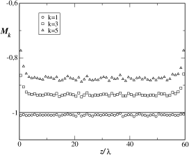
Figure 4: Steady profiles of the scaled dimensionless odd moments $M_{k}$, $k=1,3,5$, defined in Eq. (24), for a system with $L=60\lambda$. According with the theoretical prediction, $M_{k}$ should be uniform and equal to one for all $k$ odd.

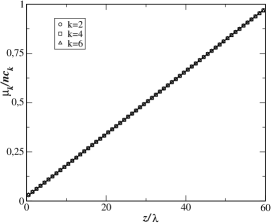
Figure 5: Steady profiles of the scaled dimensionless even moments $\mu_{k}/nc_{k}$, $k=2,4,6$, for a system with $L=60\lambda$. Also plotted (solid line) is the theoretical prediction, which is $n_{l}(z)/n$ for all $k$ even.

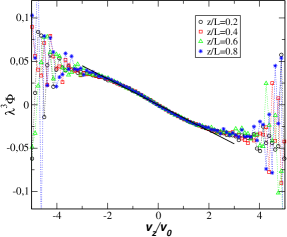
Figure 6: (Color online) Marginal velocity distribution $\Phi(z,v_{z})$ for different values of $z$ as indicated in the inset. The velocity is scaled with the thermal velocity $v_{0}=(k_{B}T/m)^{1/2}$. The symbols are simulation data for a system with $L=60\lambda$ and the solid line is the theoretical prediction given by Eq. (27).

Finally, let us consider the velocity distribution function itself. The marginal distribution for the component $z$ of the velocity, $f_{l,z}(v_{z},z)$ is defined as

$$f_{l,z}(z,v_{z})=\int d{\bm{v}}_{\perp}f_{l}(z,{\bm{v}}),$$ (25)

where the integral is carried out over those components of the velocity perpendicular to the $z$ axis. Also define

$$\Phi(z,v_{z})\equiv\frac{f_{l,z}(z,v_{z})-n_{l}(z)\varphi_{z}(v_{z})}{\varphi_{z}(v_{z})}.$$ (26)

Here $\varphi_{z}(v_{z})$ is the one-dimensional Maxwell-Boltzmann velocity distribution for $v_{z}$ with temperature $T$. The theoretical prediction in the first Sonine approximation follows directly from Eq. (18),

$$\Phi(z,v_{z})=-\frac{mDa}{k_{B}T}\,v_{z}.$$ (27)

i.e., it is independent of $z$ and linear in $v_{z}$. The first property is an exact consequence of the Boltzmann equation, while the second one is associated to the first Sonine approximation.

To measure the velocity distribution $\Phi(z,v_{z})$ in the simulations, four slices of width $\Delta z=\lambda$, located at $z=0.2L$, $0.4L$, $0.6L$, and $0.8L$ were considered. In Fig. 6 the results obtained are illustrated for the case $L=60\lambda$. The different symbols correspond to simulation data obtained at different values of $z$ as indicated in the inset. The first aspect to emphasize is that the four curves collapse, confirming that the distribution $\Phi(v_{z})$ does not depend on $z$. Moreover, the theoretical prediction, Eq. (27) is also plotted, using the slope $a$ measured in the simulations and the theoretical expression for $D$, Eq. (17). It is seen that the agreement between theory and simulation results is fairly good, especially in the thermal velocity region. On the other hand, it is true that a slight curvature is clearly identified in the simulation results. This indicates that the agreement between theory and simulation would increase probably if higher order Sonine polynomials were considered. Similar results were obtained for systems with $L=30\lambda$ and $L=90\lambda$.

4 Summary

In this paper, a steady self-diffusion process in a gas at equilibrium has been considered. The state has been shown to be predicted by the Enskog kinetic equation. Moreover, DSMC simulation results obtained under appropriate boundary conditions also indicate that the system exhibits a steady state similar to the one described by the kinetic equation. Even more, a very good quantitative agreement between the theoretical predictions and the simulation results has been found. Quite interestingly, the expressions obtained for the self-diffusion equation and for the distribution function of labeled particles to Navier-Stkes order from the Boltzmann equation, seem to hold also in the steady state, for arbitrary large gradients of labeled particles.

Exact solutions of the Boltzmann and Enskog equations are rather scarce. Moreover, self-diffusion can be considered as the prototype of transport processes and the associate self-diffusion equation as the prototype hydrodynamic equation. This includes not only usual molecular systems but also intrinsic non-equilibrium systems, as granular gases [15]. The detailed knowledge of far from equilibrium states allows to investigate the way in which hydrodynamic is approached by the system, as well as many questions related with the stability of the state and the properties of hydrodynamic fluctuations far from equilibrium. In addition, the simplicity of the exact solution reported in this paper makes it possible to address issues that are almost inaccessible otherwise.

To put the results here in a proper context, it is important to realize that they also hold for dilute gases described by the Boltzmann equation, with an arbitrary interaction potential. The Boltzmann limit of Eq.  (10) is obtained simply by putting $g_{e}(n)=1$, and the solubility condition is also verified by the Boltzmann collision operator for other interaction potentials different from hard spheres.

As a consequence of the analysis here, some relevant questions, deserving further consideration, arise. Given that the self-diffusion coefficient in the steady state agrees with the Navier-Stokes one, it means that the former is also given by the usual Green-Kubo expression. It is then interesting to see how it can be derived by considering the dynamics in the steady self-diffusion state. This requires an extension of the usual linear response theory and could be a significant first step towards the analysis of other non-equilibrium steady states.

Another important issue is whether there exist other self-diffusion steady states exhibiting different density profiles of labeled particles and, if they do, which is the relationship between them. Also, the possible generalization to dense systems described directly by the Liouville equation should be addressed as well as self-diffusion in steady non-equilibrium states.

- [1] \NameJ.R. Dorfman \BookFundamental Problems in Statistical Mechanics III \EditorE.G.D. Cohen \PublNorth-Holland, Amasterdam \Year1975 \Page277.
- [2] \NameJ.R. Dorfman H. van Beijeren \BookStatistical Medchanics, Pt.B \EditorB.J. Berne \PublPlenun Press, New York \Year1977 \Page65.
- [3] \NameP. Résibois M. de Leener \BookClassical Kinetic Theory of fluids \PublWiley, New York \Year1977.
- [4] \NameJ.A. McLennan \BookIntroduction to Non-Equilibrium Statistical Mechanics \PublPrentice-H, Englewood Cliffs, NJ \Year1989.
- [5] \NameS. Chapman T.G. Cowling \BookThe Mathematical Theory of Non-uniform Gases \PublCambridge University Press, Cambridge \Year1970.
- [6] \NameH. van Beijeren M.H. Ernst \REVIEWPhysica A681973437.
- [7] \NameJ.L. Lebowitz H. Spohn \REVIEWJ. Stat. Phys.281982539.
- [8] \NameJ.L. Lebowitz H. Spohn \REVIEWJ. Stat. Phys.29198239.
- [9] \NameC. Cercignani \BookTheory and Application of the Boltzmann Equation \PublElsevier, New York \Year1975.
- [10] \NameJ.J. Brey, M.J. Ruiz-Montero, D. Cubero R. García-Rojo \REVIEWPhysics of Fluids122000876. In this paper, a gas of inlestic particles is considered, but the elastic limit can be easily taken.
- [11] \NameA.W. LeesS.F. Edwards \REVIEWJ. Phys. C: Solid State Phys.519721921.
- [12] \NameW.T. Ashurst W.G. Hoover \REVIEWPhys. Rev. Lett.311973206.
- [13] \NameJ.J. Erpenbeck W.W. Wood \BookStatistical Mechanics, Pt. B \EditorB.J. Berne \PublPlenum Press, New York \Year1977.
- [14] \NameG. Bird \BookMolecular Gas Dynamics and the Direct Simulation of Gas Flows \PublClarendom Press, Oxford \Year1994.
- [15] \NameJ.W. Dufty, J.J. Brey, J.L. Lutsko \REVIEWPhys. Rev. E652002051303.