Chapter 1
Quantum Hall fluids in the presence of topological defects: noncommutativity, generalized magnetic translations and non-Abelian statistics

Abstract

We review our recent results on the physics of quantum Hall fluids at Jain and non conventional fillings within a general field theoretic framework. We focus on a peculiar conformal field theory (CFT), the one obtained by means of the $m$-reduction technique, and stress its power in describing strongly correlated low dimensional condensed matter systems in the presence of localized impurities or topological defects. By exploiting the notion of Morita equivalence for field theories on noncommutative two-tori and choosing rational values of the noncommutativity parameter, we find a general one-to-one correspondence between the $m$-reduced conformal field theory describing the quantum Hall fluid and an Abelian noncommutative field theory. In this way we give a meaning to the concept of ”noncommutative conformal field theory”, as the Morita equivalent version of a CFT defined on an ordinary space. In this context the image of Morita duality in the ordinary space is given by the $m$-reduction technique and the corresponding noncommutative torus Lie algebra is naturally realized in terms of generalized magnetic translations.

As an example of application of the formalism, we study a quantum Hall bilayer at nonconventional fillings in the presence of a localized topological defect and briefly recall its boundary state structure corresponding to two different boundary conditions, the periodic as well as the twisted boundary conditions respectively, which give rise to different topological sectors on a torus. By analyzing the boundary interaction terms present in the action we recognize a boundary magnetic term and a boundary potential. Then we introduce generalized magnetic translation operators as tensor products, which act on the quantum Hall fluid and defect space respectively, and compute their action on the boundary partition functions: in this way their role as boundary condition changing operators is fully evidenced. From such results we infer the general structure of generalized magnetic translations in our model and clarify the deep relation between noncommutativity and non-Abelian statistics of quasi-hole excitations, which is crucial for physical implementations of topological quantum computing. In particular, noncommutativity is strictly related to the presence of a topological defect on the edge of the bilayer system, which supports protected Majorana fermion zero modes. That happens in close analogy with point defects in topological insulators and superconductors, where the existence of Majorana bound states is related to a $Z_{2}$ topological invariant. Finally, some prospects on the implementation of a topologically protected qubit with quantum Hall bilayers are presented.

PACS 11.25.Hf, 11.10.Nx, 73.43.Cd

Keywords: Noncommutative field theory, Topological defects, Quantum Hall fluids.

1. Introduction

The experimental discovery of fractional quantum Hall (FQH) effect [1] in 1982 has opened the door to a new fascinating state of matter. Indeed the unusual properties of the incompressible quantum fluid that arises in a two dimensional electron gas subjected to a strong magnetic field and at very low temperatures are the signature of an emergent topological state of matter, whose quasiparticle excitations show up fractional charge and statistics [2][3]. As such, it has been proposed that FQH states display a new kind of order, termed topological order [4][5]. In particular they lack long range correlation and local order parameters but display a weak form of order which is sensitive to the topology of the underlying two dimensional manifold. Further appealing features are a non-Abelian Berry’s phase under modular transformations and a ground state degeneracy depending on the topology of the underlying space, which is robust against any local perturbations.

Laughlin states [6] with $\nu=\frac{1}{k}$ and $k$ odd are today well understood, both theoretically and experimentally. In order to take into account more general observed filling factors $\nu$ different from $\frac{1}{k}$, a hierarchical scheme was introduced [7], in which quasiparticles of a $\nu=\frac{1}{k}$ state can themselves condense into a new quantized state. In this way it has been possible to construct Hall states for any odd denominator filling fraction $\nu$, whose quasiparticles have fractional charge and Abelian fractional statistics. Some years later Jain introduced the composite fermions picture [8] in order to explain more general filling fractions of the form $\nu=\frac{p}{2p+1}$. The observation of a quantum Hall state with an even denominator filling fraction [9], $\nu=\frac{5}{2}$, paved the way to the study of states which do not follow the hierarchical picture and then are an exception to the odd denominator rule. The most promising theoretical candidate for such a state is believed to be the Moore-Read (MR) Pfaffian model [10], whose anyonic quasiparticles exhibit non Abelian braiding statistics. This last prediction is appealing in view of condensed matter implementations of topological quantum computation [11]. Indeed quantum information is stored in topologically degenerate states with multiple quasiparticles while unitary gate operations are carried out by braiding such quasiparticles and then by reading the corresponding states. The topological nature of these quasiparticles states makes them robust against any local perturbation. A strong support to the Moore-Read hypothesis for the $\nu=\frac{5}{2}$ state comes from recent experimental data about the charge $\frac{e}{4}$ of localized excitations [12], which coincide with previous shot noise [13] and quasiparticle interference oscillation [14] results. Further experimental evidence has been gained through the observation of the predicted neutral mode [15], also consistent with the MR picture.

At the same time, increasing technological progress in molecular beam epitaxy techniques has led to the ability to produce pairs of closely spaced two-dimensional electron gases. Since then such bilayer quantum Hall systems have been widely investigated theoretically as well as experimentally [3][16, 17]. Strong correlations between the electrons in different layers lead to new physical phenomena involving spontaneous interlayer phase coherence with an associated Goldstone mode. In particular a spontaneously broken $U(1)$ symmetry [18] has been discovered and identified and many interesting properties of such systems have been studied: the Kosterlitz-Thouless transition, the zero resistivity in the counter-current flow, a DC/AC Josephson-like effect in interlayer tunneling as well as the presence of a gapless superfluid mode [19][20]. Indeed, when tunneling between the layers is weak, the quantum Hall bilayer state can be viewed as arising from the condensation of an excitonic superfluid in which an electron in one layer is paired with a hole in the other layer. The uncertainty principle makes it impossible to tell which layer either component of this composite boson is in. Equivalently the system may be regarded as a ferromagnet in which each electron exists in a coherent superposition of the ”pseudospin” eigenstates, which encode the layer degrees of freedom [21][20]. The phase variable of such a superposition fixes the orientation of the pseudospin magnetic moment and its spatial variations govern the low energy excitations in the system. So quantum Hall bilayers are an interesting realization of the pairing picture at non-standard fillings. Indeed they show up several even denominator states.

The topological nature of quantum Hall states makes possible the classification of the different electronic phases of the quantum liquid according to topological invariants, as pioneered by Thouless [22]. He identified the integer topological invariant characterizing the two dimensional ($2D$) integer quantum Hall state, which gives the Hall conductance and characterizes the Bloch Hamiltonian defined in the magnetic Brillouin zone. As a consequence of this topological classification a bulk-boundary correspondence arises, which relates the topological class of the bulk system to the number of gapless chiral edge states on the sample boundary [4]. Topologically protected zero modes and gapless states can also occur when topological defects are present on the edge of the sample; recently a generalization of the bulk-boundary correspondence has been introduced as well [23], which relates the topological class of the Hamiltonian characterizing the defect to the structure of the protected modes associated with the defect. In this way the crucial role of localized topological defects clearly emerges and that appears to be deeply related to noncommutativity, as we showed in our recent work [24][25][26].

On the other hand, the relevance of $2D$ CFT for the fractional quantum Hall effect (FQHE) was first pointed out in Ref. [27], where the analogy between the Laughlin-Jastrow (LJ) wave function and the dual amplitudes was exploited. Then the $2D$ CFT formalism was extensively employed in the study of Hall fluids at the plateaux, assuming that it can describe successfully the universal topological features of the fractional quantum Hall effect (FQHE) [28][5]. The key point for the introduction of $2D$ CFT is the consideration that it is possible to build up a Coulomb Gas in terms of vertex operators of a $c=1$ CFT and then to compute in a natural way topological quantities such as the Hall conductance. That relies strongly on the one-component plasma interpretation of the modulus square of the Hall ground state wave function proposed by Laughlin [6]. Furthermore the vertex operator formalism describes very well states with particles carrying an electric as well as a magnetic charge, i. e. dyons. We also point out that the $2D$ CFT approach to FQHE holds not only on the plane but also on a torus [29] and in general on a Riemann surface with arbitrary genus; in this way the topological properties of the system can be made very transparent. Indeed the topological nature of the order present in the FQHE at fillings $\nu=\frac{1}{k}$ shows up as a $k$-fold degeneracy of the ground state wave function. Such a result, as well as the value of the Hall conductance, is deeply related [5] to the algebraic properties of a finite subgroup of the magnetic translation group for a $2D$ electrons system. More recently, a particular CFT, the one obtained via $m$-reduction technique [30], has been introduced by our group and applied to the description of a quantum Hall fluid (QHF) at Jain [31][32] as well as paired states fillings [33][34] and in the presence of topological defects [35][36][37]. The $m$-reduction technique is based on the simple observation that, for any CFT (mother), a class of sub-theories exists, which is parameterized by an integer $m$ with the same symmetry but different representations. The resulting theory (daughter), called Twisted Model (TM), has the same algebraic structure but a different central charge $c_{m}=mc$. Its application to the physics of the QHF arises by the incompressibility of the Hall fluid droplet at the plateaux, which implies its invariance under the $W_{1+\infty}$ algebra at different fillings [38], and by the peculiarity of the $m$-reduction procedure to provide a daughter CFT with the same $W_{1+\infty}$ invariance property of the mother theory [31][32]. Thus the $m$-reduction furnishes automatically a mapping between different incompressible plateaux of the QHF while the characteristics of the daughter theory is the presence of twisted boundary conditions on the fundamental fields.

But how noncommutativity does arise in the physics of quantum Hall regime and how does it fit to our CFT description? Really, it comes out in a very natural way as an effective description of the dynamics when the simplest framework is considered, namely the quantum mechanics of the motion of $N_{e}$ charged particles in two dimensions subjected to a transverse magnetic field (Landau problem)[39]. The strong field limit $B\rightarrow\infty$ at fixed mass $m$ projects the system onto the lowest Landau level and, for each particle $I=1,...,N_{e}$, the corresponding coordinates ($\frac{eB}{c}x_{I},y_{I}$) are a pair of canonical variables which satisfy the commutation relations $\left[x_{I},y_{I}\right]=i\delta_{I,J}\theta$, $\theta=\frac{\hbar c}{eB}\equiv l_{M}^{2}$ being the noncommutativity parameter. In this picture the electron is not a point-like particle and can be localized at best at the scale of the magnetic length $l_{M}$. The same thing happens to the endpoints of an open string attached to a $D$-brane embedded in a constant magnetic field [40], which is the string theory analogue of the Landau problem: the $D$-brane worldvolume becomes a noncommutative manifold. Indeed the worldsheet field theory for open strings attached to $D$-branes is defined by a $\sigma$-model on the string worldsheet $\Sigma$ with action

$$S_{\Sigma}=\frac{1}{4\pi l_{s}^{2}}\int_{\Sigma}d^{2}\xi\left(g_{ij}\partial^{a}y^{i}\partial_{a}y^{j}-2\pi\mathrm{i}l_{s}^{2}B_{ij}\epsilon^{ab}\partial_{a}y^{i}\partial_{b}y^{j}\right).$$ (1)

Here $y^{i}$ are the open string endpoint coordinates, $\xi^{a}$, $a=1,2$ are local coordinates on the surface $\Sigma$, $l_{s}$ is the intrinsic string length, $g_{ij}$ is the spacetime metric and $B_{ij}$ is the Neveu-Schwarz two-form which is assumed non-degenerate and can be viewed as a magnetic field on the $D$-brane. Indeed, when $B_{ij}$ are constant the second term in Eq. (1) can be integrated by parts and gives rise to the boundary action:

$$S_{\partial\Sigma}=-\frac{\mathrm{i}}{2}\int_{\partial\Sigma}dtB_{ij}y^{i}\left(t\right)\overset{.}{y}^{j}\left(t\right),$$ (2)

where $t$ is the coordinate of the boundary $\partial\Sigma$ of the string world sheet lying on the $D$-brane worldvolume and $\overset{.}{y}^{i}=\partial y^{i}/\partial t$. Such a boundary action formally coincides with the one of the Landau problem in a strong field. Now, by taking the Seiberg-Witten limit [41], i. e. by taking $g_{ij}\sim l_{s}^{4}\sim\varepsilon\rightarrow 0$ while keeping fixed the field $B_{ij}$, the effective worldsheet field theory reduces to the boundary action (2) and the canonical quantization procedure gives the commutation relations $\left[y^{i},y^{j}\right]=i\theta^{ij}$, $\theta=\frac{1}{B}$ on $\partial\Sigma$. Summarizing, the quantization of the open string endpoint coordinates $y^{i}\left(t\right)$ induces a noncommutative geometry on the $D$-brane worldvolume and the effective low-energy field theory is a noncommutative field theory (NCFT) [42] for the massless open string modes.

In such a picture also a tachyon condensation phenomenon can be considered, which introduces the following boundary interaction for the open string:

$$S_{T}=-\mathrm{i}\int_{\partial\Sigma}dtT\left(y^{i}\left(t,0\right)\right),$$ (3)

where $T\left(y^{i}\left(t,0\right)\right)$ is a general tachyon profile. In general, $D$-branes in string theory correspond to conformal boundary states, i. e. to conformally invariant boundary conditions of the associated CFT. They are charged and massive objects that interact with other objects in the bulk, for instance through exchange of higher closed string modes. In turn boundary excitations are described by fields that can be inserted only at points along the boundary, i. e. the boundary fields. There exists an infinite number of open string modes, which correspond to boundary fields in the associated boundary CFT. In other words tachyonic condensation is a boundary phenomenon and as such it is related to Kondo-like effects in condensed matter systems [43][44]. In this case, the presence of the background $B$-field makes the open string states to disappear and that explains the independence on the background [45].

The above picture coincides with the one proposed in Ref. [46] in the context of boundary conformal field theories (BCFT). The authors consider a system of two massless free scalar fields which have a boundary interaction with a periodic potential and furthermore are coupled to each other through a boundary magnetic term, whose expressions coincide with Eqs. (2) and (3). By using a string analogy, the boundary magnetic interaction allows for exchange of momentum of the open string moving in an external magnetic field. Indeed it enhances one chirality with respect to the other producing the effect of a rotation together with a scale transformation on the fields and the string parameter plays the role of dissipation. It is crucial to observe that conformal invariance of the theory is preserved only at special values of the parameters entering the action, the so called “magic” points. That happens in close analogy with the motion of an electron confined in a plane, subjected to an external magnetic field $B$, normal to the plane, and in the presence of dissipation [47]. Furthermore we have shown how our $m$-reduced theory at paired states fillings describes a dissipative system precisely at the “magic” points [36].

In this way noncommutativity comes into play and a deep relation emerges between the quantum mechanical and the string and $D$-brane description of the quantum Hall regime. Now, in order to show how it relates to our CFT description of QHF, we start by considering quantum field theories defined on a noncommutative two-torus and then resort to the concept of Morita duality [48][49][50]. Such a kind of duality establishes a relation, via a one-to-one correspondence, between representations of two noncommutative algebras and, within the context of gauge theories on noncommutative tori, it can be viewed as a low energy analogue of $T$-duality of the underlying string model [51]: as such, it results a powerful tool in order to establish a correspondence between NCFT and well known standard field theories. Indeed, for rational values of the noncommutativity parameter, $\theta=\frac{1}{N}$, one of the theories obtained by using the Morita equivalence is a commutative field theory of matrix valued fields with twisted boundary conditions and magnetic flux $c$ [52] (which, in a string description, behaves as a $B$-field modulus). Our recent work [24][25][26] strongly relies on such an idea. It aims at building up a general effective theory for QHF which could add further evidence to the relationship between the string theory picture and the condensed matter theory one as well as to the role of noncommutativity in QHF physics. In particular, we show by means of the Morita equivalence that a NCFT with $\theta=2p+\frac{1}{m}$ or $\theta=\frac{p}{2}+\frac{1}{m}$ respectively is mapped to a CFT on an ordinary space. We identify such a CFT with the $m$-reduced CFT developed for a QHF at Jain $\nu=\frac{m}{2pm+1}$ [31][32], as well as paired states fillings $\nu=\frac{m}{pm+2}$ [33][34], whose neutral fields satisfy twisted boundary conditions. Indeed the presence of a $Z_{m}$ twist is the fingerprint of a topological defect [35][36][37] localized somewhere on the edge of the system and accounts, in the open string picture, for a mismatch of momentum exchange at its two endpoints. In this way we give a meaning to the concept of ”noncommutative conformal field theory”, as the Morita equivalent version of a CFT defined on an ordinary space. The image of Morita duality in the ordinary space is given by the $m$-reduction technique and the corresponding noncommutative torus Lie algebra is naturally realized in terms of Generalized Magnetic Translations (GMT). That introduces a new relationship between noncommutative spaces and QHF and paves the way for further investigations on the role of noncommutativity in the physics of general strongly correlated many body systems [53].

In this chapter we illustrate such developments and then, as an example of application, we study in detail the physics of a system of two parallel layers of $2D$ electrons gas in a strong perpendicular magnetic field and interacting with an impurity placed somewhere on the boundary (quantum Hall bilayer). We focus on the case of non standard filling factor, which is relevant both from an experimental point of view and for possible topological quantum computing implementations. Indeed it is described by a $m$-reduced CFT with $m=2$ and we find that the $2$-reduced theory on the two-torus obtained as a Morita dual starting from a NCFT keeps track of noncommutativity in its structure. Furthermore GMT are a realization of the noncommutative torus Lie algebra. We analyze in detail the presence of a topological defect placed between the layers somewhere on the edges and discuss the relation between different defects and different possible boundary conditions by introducing the corresponding boundary partition function. A boundary state can be defined in correspondence to each class of defects [35] and a boundary partition function can be computed which corresponds to a boundary fixed point, e. g. to a different topological sector of the theory on the torus. In this context GMT are identified with operators which act on the boundary states and realize the transition between fixed points of the boundary flow. In the language of Kondo effect [44] they behave as boundary condition changing operators. We introduce general GMT operators as tensor products which act on the QHF and defect space respectively and discuss in detail their behaviour. Then, the emergence of noncommutativity as a consequence of the presence of the topological defect is emphasized and its connection with non-Abelian statistics of the quasi-hole excitations fully elucidated. We find for such excitations a $SO\left(2n\right)$ structure, typical of Ising anyons [54][55], while the topological defect supports protected Majorana fermion zero modes in close analogy with point defects in topological insulators and superconductors [23][56]. Finally we give some insights on how to build up a topologically protected qubit with a quantum Hall bilayer when two localized defects are introduced on the edge [57].

The outline of the chapter is the following.

In Section 2, we give a brief account of our theoretical approach, the $m$-reduction procedure [30], and illustrate how it works in the description of a QHF at Jain as well as paired states fillings. In this last case we discuss explicitly the $m=2$ theory, which corresponds to a quantum Hall bilayer in the presence of a localized topological defect.

Section 3 is devoted to show how noncommutativity comes into play in our CFT description by focusing on the issue of Morita equivalence for field theories on noncommutative two-tori. That allows us to introduce a new relationship between noncommutative spaces and QHF, which is explicitly discussed for Jain $\nu=\frac{m}{2pm+1}$ [31][32], as well as paired states fillings $\nu=\frac{m}{pm+2}$ [33][34]. In this last case we make explicit reference to the bilayer theory $m=2$, which will be the subject of our study in the following Sections.

In Section 4 we focus on the physics of a quantum Hall bilayer at paired states fillings because it is the simplest non trivial example on which all the relevant features of our theory can be exploited. We discuss in detail the different possible boundary interactions of the system and show how it is equivalent to a system of two massless scalar bosons with a magnetic boundary interaction at particular points [46]. Then the boundary content of our theory is rephrased in terms of boundary partition functions, which are shown to be closed upon action of GMT. These results allow us to infer the structure of the most general GMT operators.

In Section 5 we present and discuss in detail the structure of GMT for quantum Hall bilayers as tensor products acting on the QHF and defect space respectively. In particular we find an interesting relation between noncommutativity and non-Abelian statistics of quasihole excitations, as a consequence of the presence of a defect. Finally we briefly sketch a possible implementation of a topologically protected qubit with two localized defects introduced on the edge of the bilayer system.

In Section 6, some comments and outlooks of our work are given.

Finally, the operator content of our theory, the TM, on the torus for a quantum Hall bilayer at paired states fillings is recalled in the Appendix.

2. The $m$-reduction technique

In this Section we briefly review the basics of the $m$-reduction procedure on the plane (genus $g=0$) [30] and then we show how it works, referring to the description of a QHF at Jain $\nu=\frac{m}{2pm+1}$ [31][32] as well as paired states fillings $\nu=\frac{m}{pm+2}$ [33][34].

In general, the $m$-reduction technique is based on the simple observation that for any CFT (mother) exists a class of sub-theories parameterized by an integer $m$ with the same symmetry but different representations. The resulting theory (daughter) has the same algebraic structure but a different central charge $c_{m}=mc$. In order to obtain the generators of the algebra in the new theory we need to extract the modes which are divided by the integer $m$. These can be used to reconstruct the primary fields of the daughter CFT. This technique can be generalized and applied to any extended chiral algebra which includes the Virasoro one. Following this line one can generate a large class of CFTs with the same extended symmetry but with different central extensions. It can be applied in particular to describe the full class of Wess-Zumino-Witten (WZW) models with symmetry $\widehat{su(2)}_{m}$, obtaining the associated parafermions in a natural way or the incompressible $W_{1+\infty}$ minimal models [38] with central charge $c=m$. Indeed the $m$-reduction preserves the commutation relations between the algebra generators but modify the central extension (i.e. the level for the WZW models). In particular this implies that the number of the primary fields gets modified.

The general characteristics of the daughter theory is the presence of twisted boundary conditions (TBC) which are induced on the component fields and are the signature of an interaction with a localized topological defect. It is illuminating to give a geometric interpretation of that in terms of the covering on a $m$-sheeted surface or complex curve with branch-cuts, see for instance Figs. 1, 2 for the particular case $m=2$.

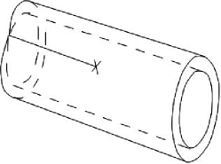
Figure 1.: The edge of the $2$-covered cylinder can be viewed as a separation line of two different domains of the $2$-reduced CFT.

Indeed the fields which are defined on the left domain of the boundary have TBC while the fields defined on the right one have periodic boundary conditions (PBC). When we generalize the construction to a Riemann surface of genus $g=1$, i. e. a torus, we find different sectors corresponding to different boundary conditions on the cylinder, as shown in detail in Refs. [32][34]. Finally we recognize the daughter theory as an orbifold of the usual CFT describing the QHF at a given plateau.

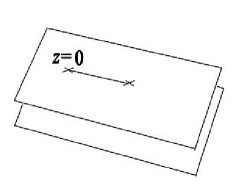
Figure 2.: The local branched plane.

The physical interpretation of such a construction within the context of a QHF description is the following. The two sheets simulate a two-layer quantum Hall system and the branch cut represents TBC which emerge from the interaction with a localized topological defect on the edge [35][36][37].

Let us now briefly summarize our $m$-reduction procedure on the plane [30]. The starting point is described by a CFT with $c=1$, in terms of a scalar chiral field compactified on a circle with general radius $R^{2}$ ($R^{2}=1$ for the Jain series [31] while $R^{2}=2$ for the non standard one [33], as we will recall in the following). Then the $u(1)$ current is given by $J(z)=i\partial_{z}Q(z)$, where $Q(z)$ is the compactified Fubini field with the standard mode expansion:

$$Q(z)=q-i\,p\,lnz+\sum_{n\neq 0}\frac{a_{n}}{n}z^{-n},$$ (4)

where $a_{n}$, $q$ and $p$ satisfy the commutation relations $\left[a_{n},a_{n^{\prime}}\right]=n\delta_{n,n^{\prime}}$ and $\left[q,p\right]=i$. The primary fields are expressed in terms of the vertex operators $U^{\alpha_{s}}(z)=:e^{i\alpha_{s}Q(z)}:$ with $\alpha_{s}=\frac{s}{R}$ ($s=1,...,R^{2}$) and conformal dimension $h=\frac{s^{2}}{2R^{2}}$.

Starting with the set of fields in the above CFT and using the $m$-reduction procedure, which consists in considering the subalgebra generated only by the modes in Eq. (4), which are multiple of an integer $m$, we get the image of the twisted sector of a $c=m$ orbifold CFT (i. e. the TM), which describes the Lowest Landau Level (LLL) dynamics of the new filling in the QHF context. In this way the fundamental fields are mapped into $m$ twisted fields which are related by a discrete Abelian group. Indeed the fields in the mother CFT can be factorized into irreducible orbits of the discrete $Z_{m}$ group, which is a symmetry of the TM, and can be organized into components, which have well defined transformation properties under this group. To compare the orbifold so built with the $c=m$ CFT, we use the mapping $z\rightarrow z^{1/m}$ and the isomorphism, defined in Ref. [30], between fields on the $z$ plane and fields on the $z^{m}$ covering plane given by the following identifications: $a_{nm+l}\longrightarrow\sqrt{m}a_{n+l/m}$, $q\longrightarrow\frac{1}{\sqrt{m}}q$.

We perform a “double” $m$-reduction which consists in applying this technique into two steps.

1) The $m$-reduction is applied to the Fubini field $Q(z).$ That induces twisted boundary conditions on the currents. It is useful to define the invariant scalar field:

$$X(z)=\frac{1}{m}\sum_{j=1}^{m}Q(\varepsilon^{j}z),$$ (5)

where $\varepsilon^{j}=e^{i\frac{2\pi j}{m}}$, corresponding to a compactified boson on a circle with radius now equal to $R_{X}^{2}=R^{2}/m$. This field describes the $U(1)$ electrically charged component of the new filling in a QHF description.

On the other hand the non-invariant fields defined by

$$\phi^{j}(z)=Q(\varepsilon^{j}z)-X(z),~{}~{}~{}~{}~{}~{}~{}~{}~{}~{}~{}~{}~{}~{}~{}~{}\sum_{j=1}^{m}\phi^{j}(z)=0$$ (6)

naturally satisfy twisted boundary conditions, so that the $J(z)$ current of the mother theory decomposes into a charged current given by $J(z)=i\partial_{z}X(z)$ and $m-1$ neutral ones $\partial_{z}\phi^{j}(z)$.

2) The $m$-reduction applied to the vertex operators $U^{\alpha_{s}}(z)$ of the mother theory also induces twisted boundary conditions on the vertex operators of the daughter CFT. The discrete group used in this case is just the $m$-ality group which selects the neutral modes with a complementary cut singularity, which is necessary to reinforce the locality constraint.

The vertex operator in the mother theory can be factorized into a vertex that depends only on the $X(z)$ field:

$$\mathcal{U}^{\alpha_{s}}(z)=z^{\frac{\alpha_{s}^{2}(m-1)}{m}}:e^{i\alpha_{s}{\ }X(z)}:$$ (7)

and in vertex operators depending on the $\phi^{j}(z)$ fields. It is useful to introduce the neutral component:

$$\psi_{1}(z)=\frac{z^{\frac{1-m}{m}}}{m}\sum_{j=1}^{m}\varepsilon^{j}:e^{i\phi^{j}(z)}:$$ (8)

which is invariant under the twist group given in 1) and has $m$-ality charge $l=1$. Then, the new primary fields are the composite vertex operators $V^{\alpha_{s}}(z)=\mathcal{U}^{\alpha_{s}}(z)\psi_{l}(z)$, where $\psi_{l}$ are the neutral operators with $m$-ality charge $l$.

From these primary fields we can obtain the new Virasoro algebra with central charge $c=m$ which is generated by the energy-momentum tensor $T(z)$. It is the sum of two independent operators, one depending on the charged sector:

$$T_{X}(z)=-\frac{1}{2}:\left(\partial_{z}X\left(z\right)\right)^{2}:$$ (9)

with $c=1$ and the other given in terms of the $Z_{m}$ twisted bosons $\phi^{j}(z)$:

$$T_{\phi}(z)=-\frac{1}{2}\sum_{j,j^{\prime}=1}^{m}:\partial_{z}\phi^{j}(z)\partial_{z}\phi^{j^{\prime}}(z):+\ \frac{m^{2}-1}{24mz^{2}}$$ (10)

with $c=m-1$.

Let us notice here that, although the daughter CFT has the same central charge value, it differs in the symmetry properties and in the spectrum, depending on the mother theory we are considering, i.e. for Jain [31] or non standard series [33] in the case of a QHF as we will show in the following.

2.1. Jain fillings

In this Subsection we focus on the description of a QHF at Jain fillings in terms of vertex operators and review the main results of $m$-reduction procedure in order to classify its excitations. The starting point is a CFT with $c=1$, in terms of a scalar chiral field compactified on a circle with radius $R^{2}=1$. Then the $U(1)$ current is given by $J(z)=i\partial_{z}Q(z)$, where $Q(z)$ is the compactified Fubini field given in Eq. (4). The primary fields are expressed in terms of the vertex operators $U^{\alpha_{s}}(z)=:e^{i\alpha_{s}Q(z)}:$ with $s=1$ and conformal dimension $h=\frac{1}{2}$. The dynamical symmetry is given by the $W_{1+\infty}$ algebra [58] with $c=1$, whose generators are simply given by a power of the current $J(z)$. By using the $m$-reduction procedure, we get the image of the twisted sector of a $c=m$ orbifold CFT which has $\widehat{U}(1){\times}\widehat{SU}(m)_{1}$ as extended symmetry and describes the QHF at the new general filling $\nu=\frac{m}{2pm+1}$. In order to do so, we factorize the fields into two parts, the first is the $c_{X}=1$ charged sector with radius $R_{X}^{2}=\frac{2pm+1}{m}$, the second describes neutral excitations with total conformal central charge $c_{\phi}=m-1$ for any $p\in N$ [31].

In order to obtain a pure holomorphic wave function we have to consider the correlator of the TM primary fields, which are the composite vertex operators $V^{\alpha_{s}}(z)=\mathcal{U}^{\alpha_{s}}(z)\psi_{l}(z)$ with conformal dimension:

$$h_{l}=\frac{l^{2}}{2m\left(2pm+1\right)}+\frac{a}{2}\left(\frac{m-a}{m}\right),\text{ \ \ \ \ \ \ \ \ }l=1,2,...,m\left(2pm+1\right);$$ (11)

they describe excitations with electric charge $q_{e}=\frac{l}{2pm+1}$ and magnetic charge $q_{m}=l$ in units of $\frac{hc}{e}$. There exist also integer charge quasi-particles (termed $a$-electrons), with half integer (or integer) conformal dimension given by:

$$h_{l}=a^{2}p+\frac{a}{2},\text{ \ \ \ \ \ \ \ \ }l=\left(2pm+1\right)a;\text{ \ \ \ \ \ \ \ }a=1,2,...,m.$$ (12)

In particular the electrons are obtained in correspondence of $q_{e}=1$ and $q_{m}=2pm+1$, while the other $2pm$ primary fields correspond to anyons.

The spectrum just obtained follows from the construction of the Virasoro algebra with central charge $c=m$ (see Eqs. (9)-(10)). We should point out that $m$-ality in the neutral sector is coupled to the charged one exactly, as it was derived in Refs. [59][38] according to the physical request of locality of the electrons with respect to the edge excitations. Indeed our projection, when applied to a local field (namely the electron field in the case of filling factor $\nu=1$), automatically couples the discrete $Z_{m}$ charge of $U(1)$ with the neutral sector in order to give rise to a well defined, i. e. single valued, composite field. Let us also notice that the $m$-electron vertex operator does not contain any neutral field, so its wave function is realized only by means of the $c_{X}=1$ charged sector: we deal with a pseudoparticle with electric charge $m$ and magnetic charge $2pm+1$. The above construction has been generalized to the torus topology as well [32], confirming the picture just outlined for the spectrum of excitations of a QHF at Jain fillings.

2.2. Paired states fillings

Let us now review how the $m$-reduced theory describes successfully a QHF at paired states fillings $\nu=\frac{m}{pm+2}$ [33, 34]. We focus mainly on the special case $m=2$ and on the physics of a quantum Hall bilayer, which will be of our interest in the following sections as a case study to illustrate the main theoretical developments we are going to present in this paper.

The idea is to build up an unifying theory for all the plateaux with even denominator starting from the bosonic Laughlin filling $\nu=1/pm+2$, which is described by a CFT with $c=1$, in terms of a scalar chiral field compactified on a circle with radius $R^{2}=1/\nu=pm+2$ (or the dual $R^{2}=4/pm+2$). Then the $U(1)$ current is given by $J(z)=i\partial_{z}Q(z)$, where $Q(z)$ is the compactified Fubini field with the standard mode expansion (4). Let us notice that the informations about the quantization of momentum and the winding numbers are stored in the lattice geometry induced by the QHE quantization (see Ref. [33] for details); in other words the QHE physics fixes the compactification radius. The corresponding primary fields are expressed in terms of the vertex operators $U^{\alpha}(z)=:e^{i\alpha Q(z)}:$ with $\alpha^{2}=1,...,2+pm$ and conformal dimension $h=\frac{\alpha^{2}}{2}$. Also here, as for Jain fillings, starting with this set of fields and using the $m$-reduction procedure, we get the image of the twisted sector of a $c=m$ orbifold CFT, which describes the lowest Landau level dynamics.

Let us now concentrate on the special $m=2$ case, which describes a system consisting of two parallel layers of $2D$ electrons gas in a strong perpendicular magnetic field. The filling factor $\nu^{(a)}=\frac{1}{2p+2}$ is the same for the two $a=1$, $2$ layers while the total filling is $\nu=\nu^{(1)}+\nu^{(2)}=\frac{1}{p+1}$. For $p=0$ ($p=1$) it describes the bosonic $220$ (fermionic $331$) Halperin (H) state [60].

The CFT description for such a system can be given in terms of two compactified chiral bosons $Q^{(a)}$ with central charge $c=2$. In order to construct the fields $Q^{(a)}$ for the TM, the starting point is the bosonic filling $\nu=1/2(p+1)$, described by a CFT with $c=1$ in terms of a scalar chiral field $Q$ compactified on a circle with radius $R^{2}=1/\nu=2(p+1)$ (or its dual $R^{2}=2/(p+1)$), see Eq. (4). The $m$-reduction procedure generates a daughter theory which is a $c=2$ orbifold. Its primary fields content can be expressed in terms of a $Z_{2}$-invariant scalar field $X(z)$, given by

$$X(z)=\frac{1}{2}\left(Q^{(1)}(z)+Q^{(2)}(-z)\right),$$ (13)

describing the electrically charged sector of the new filling, and a twisted field

$$\phi(z)=\frac{1}{2}\left(Q^{(1)}(z)-Q^{(2)}(-z)\right),$$ (14)

which satisfies the twisted boundary conditions $\phi(e^{i\pi}z)=-\phi(z)$ and describes the neutral sector [33]. Such TBC signal the presence of a localized topological defect which couples the $2$ edges in such a way to get a crossing, as sketched in Fig. 3.

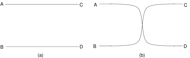
Figure 3.: The bilayer system, (a) without the topological defect (PBC), (b) with the topological defect (TBC).

The chiral fields $Q^{(a)}$, defined on a single layer $a=1$, $2$, due to the boundary conditions imposed upon them by the orbifold construction, can be thought of as components of a unique “boson” defined on a double covering of the disc (layer) ($z_{i}^{(1)}=-z_{i}^{(2)}=z_{i}$). As a consequence the two layers system becomes equivalent to one-layer QHF (in contrast with the Halperin model in which they appear independent) and the $X$ and $\phi$ fields defined in Eqs. (13) and (14) diagonalize the interlayer interaction. In particular the $X$ field carries the total charge with velocity $v_{X}$, while $\phi$ carries the charge difference of the two edges with velocity $v_{\phi}$, i.e. no charge, being the number of electrons the same for each layer (balanced system).

The primary fields are the composite operators $V(z)=\mathcal{U}_{X}(z)\psi(z)$, where $\mathcal{U}_{X}(z)=\frac{1}{\sqrt{z}}:e^{i\alpha X(z)}:$ are the vertices of the charged sector with $\alpha^{2}=2(p+1)$. Furthermore the highest weight states of the neutral sector can be classified in terms of two kinds of chiral operators, $\psi(z)\left(\bar{\psi}(z)\right)=\frac{1}{2\sqrt{z}}\left(e^{i\alpha{\cdot}\phi(z)}\pm e^{i\alpha{\cdot}\phi(-z)}\right)$, which, in a fermionic language, correspond to $c=1/2$ Majorana fermions with periodic (Ramond) or anti-periodic (Neveu-Schwarz) boundary conditions [34]. As a consequence this theory decomposes into a tensor product of two CFTs, a twisted invariant one with $c=3/2$, realized by the charged boson $X(z)$ and the Ramond Majorana fermion, which is coupled to the charged sector, while the second one has $c=1/2$ and is realized in terms of the Neveu-Schwarz Majorana fermion. The two Majorana fermions just defined are inequivalent, due to the breaking of the symmetry which exchanges them, and that results in a non-Abelian statistics. Such a factorization is much more evident in the construction of the modular invariant partition function, as we briefly recall in the Appendix [34]. The bosonized energy-momentum tensor of the $Z_{2}$ twist invariant theory develops a cosine term in its neutral sector which is described by the Ramond fields:

$$T_{\psi_{s}}(z)=-\frac{1}{4}(\partial\phi)^{2}-\frac{1}{16z^{2}}\cos(2\sqrt{2}\phi).$$ (15)

It is a clear signature of a tunneling phenomenon which selects out a new stable vacuum, the $c=3/2$ one. If we refer to the bilayer system, we can reduce the spacing between the layers so that the two species of electrons which live on them become indistinguishable: in such a case the tunneling amplitude gets large enough to make the H states flow to the Moore-Read (MR) states [10]. In the limit of strong tunneling the velocity of one Majorana becomes zero and the theory reduces to the $c=3/2$ CFT. Let us also point out that $m$-ality in the neutral sector is coupled to the charged one exactly, according to the physical request of locality of the electrons with respect to the edge excitations. Indeed our projection, when applied to a local field, automatically couples the discrete $Z_{m}$ charge of $U(1)$ with the neutral sector in order to give rise to a single valued composite field.

Now let us give an interpretation of the existence of these sectors in terms of conformal invariant boundary conditions which are due to the scattering of the particles on localized impurities [35][36][37]. The H sector describes a pure QHF phase in which  no impurities are present and the two layers edges are not connected (see Fig. 3(a)). In realistic samples however this is not the case and the deviations from the Halperin state may be regarded as due to the presence of localized impurities. These effects can be accounted for by allowing for more general boundary conditions just as the ones provided by our TM. In fact an impurity located at a given point on the edge induces twisted boundary conditions for the boson $\phi$ and, as a consequence, a current can flow between the layers. Then a coherent superposition of interlayer interactions could drive the bilayer to a more symmetric phase in which the two layers are indistinguishable due to the presence of a one electron tunneling effect along the edge.

The primary fields content of the theory just introduced on the torus topology will be given in the Appendix.

3. m-reduction, noncommutativity and Morita equivalence

In this Section we show how the issue of noncommutativity enters our CFT description for QHF by fully exploiting the notion of Morita equivalence on noncommutative tori; as we will see, it will be crucial to choose rational values of the noncommutativity parameter $\theta$. That allows us to build up a general isomorphism between NCFTs and CFTs on the ordinary space. We will make an explicit reference to the $m$-reduced theory describing a QHF at Jain and paired states fillings, recalled in Section 2. We obtain two main results: i) from a theoretical perspective, a new characterization of the $m$-reduction procedure is derived, as the image in the ordinary space of Morita duality; ii) from a more applicative perspective, a new relationship emerges between noncommutativity and QHF physics. Furthermore the noncommutative torus Lie algebra is naturally realized, within the QHF context, in terms of GMT.

The Morita equivalence [48][50] is an isomorphism between noncommutative algebras that conserves all the modules and their associated structures. Let us consider an $U(N)$ NCFT defined on the noncommutative torus $\mathrm{T}_{\theta}^{2}$ and, for simplicity, of radii $R$. The coordinates satisfy the commutation rule $[x_{1},x_{2}]=i\theta$ [42]. In such a simple case the Morita duality is represented by the following $SL(2,Z)$ action on the parameters:

$$\theta^{{}^{\prime}}=\frac{a\theta+b}{c\theta+d};\text{ \ \ \ \ \ \ \ \ }R^{{}^{\prime}}=\left|c\theta+d\right|R,$$ (16)

where $a,b,c,d$ are integers and $ad-bc=1$.

For rational values of the non commutativity parameter, $\theta=-\frac{b}{a}$, so that $c\theta+d=\frac{1}{a}$, the Morita transformation (16) sends the NCFT to an ordinary one with $\theta^{{}^{\prime}}=0$ and different radius $R^{{}^{\prime}}=\frac{R}{a}$, involving in particular a rescaling of the rank of the gauge group [61][62][63][64]. Indeed the dual theory is a twisted $U(N^{{}^{\prime}})$ theory with $N^{{}^{\prime}}=aN$. The classes of $\theta^{{}^{\prime}}=0$ theories are parametrized by an integer $m$, so that for any $m$ there is a finite number of Abelian theories which are related by a subset of the transformations given in Eq. (16). This is a crucial remark as we will show in the following, for CFT theories describing QHF at Jain as well as paired states fillings, respectively.

3.1. Jain fillings

Let us show in detail how Morita duality works for Jain fillings. Indeed the $m$-reduction technique applied to the QHF at Jain fillings ($\nu=\frac{m}{2pm+1}$) can be viewed as the image of the Morita map (characterized by $a=2p(m-1)+1$, $b=2p$, $c=m-1$, $d=1$) between the two NCFTs with $\theta=1$ and $\theta=2p+\frac{1}{m}$ respectively and corresponds to the Morita map in the ordinary space. The $\theta=1$ theory is an $U\left(1\right)_{\theta=1}$ NCFT while the mother CFT is an ordinary $U\left(1\right)$ theory; furthermore, when the $U\left(1\right)_{\theta=2p+\frac{1}{m}}$ NCFT is considered, its Morita dual CFT has $U\left(m\right)$ symmetry. As a consequence, the following correspondence Table between the NCFTs and the ordinary CFTs is established:

$$\begin{array}[]{ccc}&\text{Morita}&\\ U\left(1\right)_{\theta=1}&\rightarrow&U\left(1\right)_{\theta=0}\\ &\left(a=1,b=-1,c=0,d=1\right)&\\ \text{Morita}\downarrow\left(a,b,c,d\right)&&m-\text{reduction}\downarrow\\ &\text{Morita}&\\ U\left(1\right)_{\theta=2p+\frac{1}{m}}&\rightarrow&U\left(m\right)_{\theta=0}\\ &\left(a=m,b=-2pm-1,c=1-m,d=2p\left(m-1\right)+1\right)&\end{array}$$ (17)

For more general commutativity parameters $\theta=\frac{q}{m}$ such a correspondence can be easily extended. Indeed the action of the $m$-reduction procedure on the number $q$ doesn’t change the central charge of the CFT under study but modifies the compactification radius of the charged sector [31][32]. Nevertheless here we are interested to the action of the Morita map on the denominator of the parameter $\theta$ which has interesting consequences on noncommutativity, so in the following we will concentrate on such an issue.

In order to show that the $m$-reduction technique applied to the QHF at Jain fillings is the image of the Morita map between the two NCFTs with $\theta=1$ and $\theta=2p+\frac{1}{m}$ respectively and corresponds to the Morita map in the ordinary space it is enough to show how the twisted boundary conditions on the neutral fields of the $m$-reduced theory (see Section 2) arise as a consequence of the noncommutative nature of the $U\left(1\right)_{\theta=2p+\frac{1}{m}}$ NCFT.

In order to carry out this program let us recall that an associative algebra of smooth functions over the noncommutative two-torus $\mathrm{T}_{\theta}^{2}$ can be realized through the Moyal product ($\left[x_{1},x_{2}\right]=i\theta$):

$$f\left(x\right)\ast g\left(x\right)=\left.\exp\left(\frac{i\theta}{2}\left(\partial_{x_{1}}\partial_{y_{2}}-\partial_{x_{2}}\partial_{y_{1}}\right)\right)f\left(x\right)g\left(y\right)\right|_{y=x}.$$ (18)

It is convenient to decompose the elements of the algebra, i. e. the fields, in their Fourier components. However a general field operator $\Phi$ defined on a torus can have different boundary conditions associated to any of the compact directions. For the torus we have four different possibilities:

$$\begin{array}[]{cc}\Phi\left(x_{1}+R,x_{2}\right)=e^{2\pi i\alpha_{1}}\Phi\left(x_{1},x_{2}\right),&\Phi\left(x_{1},x_{2}+R\right)=e^{2\pi i\alpha_{2}}\Phi\left(x_{1},x_{2}\right),\end{array}$$ (19)

where $\alpha_{1}$ and $\alpha_{2}$ are the boundary parameters. The Fourier expansion of the general field operator $\Phi_{\overrightarrow{\alpha}}$ with boundary conditions $\overrightarrow{\alpha}=\left(\alpha_{1},\alpha_{2}\right)$ takes the form:

$$\Phi_{\overrightarrow{\alpha}}=\sum_{\overrightarrow{n}}\Phi^{\overrightarrow{n}}U_{\overrightarrow{n}+\overrightarrow{\alpha}}$$ (20)

where we define the generators as

$$U_{\overrightarrow{n}}\equiv\exp\left(2\pi i\frac{\overrightarrow{n}\cdot\overrightarrow{x}}{R}\right).$$ (21)

They give rise to the following commutator:

$$\left[U_{\overrightarrow{n}+\overrightarrow{\alpha}},U_{\overrightarrow{n^{\prime}}+\overrightarrow{\alpha^{\prime}}}\right]=-2i\sin\left(\frac{2\pi^{2}\theta}{R^{2}}\left(\overrightarrow{n}+\overrightarrow{\alpha}\right)\wedge\left(\overrightarrow{n^{\prime}}+\overrightarrow{\alpha^{\prime}}\right)\right)U_{\overrightarrow{n}+\overrightarrow{n^{\prime}}+\overrightarrow{\alpha}+\overrightarrow{\alpha^{\prime}}},$$ (22)

where $\overrightarrow{p}\wedge\overrightarrow{q}=\varepsilon_{ij}p_{i}q_{j}$.

When the noncommutativity parameter $\theta$ takes the rational value $\theta=\frac{2q}{m}\frac{R^{2}}{2\pi}$, being $q$ and $m$ relatively prime integers, the infinite-dimensional algebra generated by the $U_{\overrightarrow{n}+\overrightarrow{\alpha}}$ breaks up into equivalence classes of finite dimensional subspaces. Indeed the elements $U_{m\overrightarrow{n}}$ generate the center of the algebra and that makes possible for the momenta the following decomposition:

$$\overrightarrow{n^{\prime}}+\overrightarrow{\alpha}=m\overrightarrow{n}+\overrightarrow{n},\text{ \ \ \ \ }0\leq n_{1},n_{2}\leq m-1.$$ (23)

The whole algebra splits into equivalence classes classified by all the possible values of $m\overrightarrow{n}$, each class being a subalgebra generated by the $m^{2}$ functions $U_{\overrightarrow{n}+\overrightarrow{\alpha}}$ which satisfy the relations

$$\left[U_{\overrightarrow{n}+\overrightarrow{\alpha}},U_{\overrightarrow{n^{\prime}}+\overrightarrow{\alpha^{\prime}}}\right]=-2i\sin\left(\frac{\pi q}{m}\left(\overrightarrow{n}+\overrightarrow{\alpha}\right)\wedge\left(\overrightarrow{n^{\prime}}+\overrightarrow{\alpha^{\prime}}\right)\right)U_{\overrightarrow{n}+\overrightarrow{n^{\prime}}+\overrightarrow{\alpha}+\overrightarrow{\alpha^{\prime}}}.$$ (24)

The algebra (24) is isomorphic to the (complexification of the) $U\left(m\right)$ algebra, whose general $m$-dimensional representation can be constructed by means of the following ”shift” and ”clock” matrices [65][66]:

$$\mathrm{Q}=\left(\begin{array}[]{cccc}1&&&\\ &\varepsilon&&\\ &&\ddots&\\ &&&\varepsilon^{m-1}\end{array}\right),\text{ \ \ \ \ \ \ }\mathrm{P}=\left(\begin{array}[]{cccc}0&1&&0\\ &\cdots&&\\ &&\vdots&1\\ 1&&&0\end{array}\right),$$ (25)

being $\varepsilon=\exp(\frac{2\pi iq}{m})$. So the matrices $J_{\overrightarrow{n}}=\varepsilon^{n_{1}n_{2}}\mathrm{Q}^{n_{1}}\mathrm{P}^{n_{2}}$, $n_{1},n_{2}=0,...,m-1$, generate an algebra isomorphic to (24):

$$\left[J_{\overrightarrow{n}},J_{\overrightarrow{n^{\prime}}}\right]=-2i\sin\left(\pi\frac{q}{m}\overrightarrow{n}\wedge\overrightarrow{n^{\prime}}\right)J_{\overrightarrow{n}+\overrightarrow{n^{\prime}}}.$$ (26)

Thus the following Morita mapping has been realized between the Fourier modes defined on a noncommutative torus and functions taking values on $U\left(m\right)$ but defined on a commutative space:

$$\exp\left(2\pi i\frac{\left(\overrightarrow{n}+\overrightarrow{\alpha}\right)\cdot\widehat{\overrightarrow{x}}}{R}\right)\longleftrightarrow\exp\left(2\pi i\frac{\left(\overrightarrow{n}+\overrightarrow{\alpha}\right)\cdot\overrightarrow{x}}{R}\right)J_{\overrightarrow{n}+\overrightarrow{\alpha}}.$$ (27)

As a consequence a mapping between the fields $\Phi_{\overrightarrow{\alpha}}$ is generated as follows. Let us focus, for simplicity, on the case $q=1$ which leads for the momenta to the decomposition $\overrightarrow{n}=m\overrightarrow{n}+\overrightarrow{j}$, with     $0\leq j_{1},j_{2}\leq m$. The general field operator $\Phi_{\overrightarrow{\alpha}}$ on the noncommutative torus $\mathrm{T}_{\theta}^{2}$ with boundary conditions $\overrightarrow{\alpha}$ can be written in the form:

$$\Phi_{\overrightarrow{\alpha}}=\sum_{\overrightarrow{n}}\exp\left(2\pi im\frac{\overrightarrow{n}\cdot\overrightarrow{x}}{R}\right)\sum_{\overrightarrow{j}=0}^{m^{\prime}-1}\Phi^{\overrightarrow{n},\overrightarrow{j}}U_{\overrightarrow{j}+\overrightarrow{\alpha}}.$$ (28)

By using Eq. (27) we obtain the Morita correspondence between fields as:

$$\Phi_{\overrightarrow{\alpha}}\longleftrightarrow\Phi=\sum_{\overrightarrow{j}=0}^{m^{\prime}-1}\chi^{\left(\overrightarrow{j}\right)}J_{\overrightarrow{j}+\overrightarrow{\alpha}},$$ (29)

where we have defined:

$$\chi^{\left(\overrightarrow{j}\right)}=\exp\left(2\pi i\frac{\left(\overrightarrow{j}+\overrightarrow{\alpha}\right)\cdot\overrightarrow{x}}{R}\right)\sum_{\overrightarrow{n}}\Phi^{\overrightarrow{n},\overrightarrow{j}}\exp\left(2\pi im\frac{\overrightarrow{n}\cdot\overrightarrow{x}}{R}\right).$$ (30)

The field $\Phi$ is defined on the dual torus with radius $R^{\prime}=\frac{R}{m^{\prime}}$ and satisfies the boundary conditions:

$$\begin{array}[]{cc}\Phi\left(\theta+R^{\prime},x_{2}\right)=\Omega_{1}^{+}\cdot\Phi\left(\theta,x_{2}\right)\cdot\Omega_{1},&\Phi\left(\theta,x_{2}+R^{\prime}\right)=\Omega_{2}^{+}\cdot\Phi\left(\theta,x_{2}\right)\cdot\Omega_{2},\end{array}$$ (31)

with

$$\Omega_{1}=\mathrm{P}^{b},\text{ \ \ \ \ \ \ }\Omega_{2}=\mathrm{Q}^{1/q},$$ (32)

where $b$ is an integer satisfying $am-bq=1$. While the field components $\chi^{\left(\overrightarrow{j}\right)}$ satisfy the following twisted boundary conditions:

$$\begin{array}[]{c}\chi^{\left(\overrightarrow{j}\right)}\left(\theta+R^{\prime},x_{2}\right)=e^{2\pi i\left(j_{1}+\alpha_{1}\right)/m}\chi^{\left(\overrightarrow{j}\right)}\left(\theta,x_{2}\right)\\ \chi^{\left(\overrightarrow{j}\right)}\left(\theta,x_{2}+R^{\prime}\right)=e^{2\pi i\left(j_{2}+\alpha_{2}\right)/m}\chi^{\left(\overrightarrow{j}\right)}\left(\theta,x_{2}\right)\end{array},$$ (33)

that is

$$\left(\frac{j_{1}+\alpha_{1}}{m},\frac{j_{2}+\alpha_{2}}{m}\right),\text{ \ \ \ \ }j_{1}=0,...,m-1,\text{ \ \ \ \ }j_{2}=0,...,m-1.$$ (34)

Let us observe that $\overrightarrow{j}=\left(0,0\right)$ is the trace degree of freedom which can be identified with the $U(1)$ component of the matrix valued field or the charged component within the $m$-reduced theory of the QHF at Jain fillings introduced in Section 2. We infer that only the integer part of $\frac{n_{i}}{m}$ should really be thought of as the momentum. The commutative torus is smaller by a factor $m\times m$ than the noncommutative one; in fact, upon this rescaling, also the ”density of degrees of freedom” is kept constant as now we are dealing with $m\times m$ matrices instead of scalars.

Summarizing, when the parameter $\theta$ is rational we recover the whole structure of the noncommutative torus and recognize the twisted boundary conditions which characterize the neutral fields (6) of the $m$-reduced theory as the consequence of the Morita mapping of the starting NCFT ($U\left(1\right)_{\theta=2p+\frac{1}{m}}$ in our case) on the ordinary commutative space. Indeed $\chi^{\left(0,0\right)}$ corresponds to the charged $X$ field while the twisted fields $\chi^{\left(\overrightarrow{j}\right)}$ with $\overrightarrow{j}\neq\left(0,0\right)$ should be identified with the neutral ones (6). Therefore the $m$-reduction technique can be viewed as a realization of the Morita mapping between NCFTs and CFTs on the ordinary space, as sketched in the Table (17).

Let us now complete the proof by introducing generalized magnetic translations which realize the noncommutative torus Lie algebra defined in Eq. (24). In order to define GMT let us point out that, in our TM model for the QHF (see Section 2 and Refs. [31],[32],[33],[34]), the primary fields (and then the corresponding characters within the torus topology) appear as composite field operators which factorize in a charged as well as a neutral part. Further they are also coupled by the discrete symmetry group $Z_{m}$. This decomposition must hold for magnetic translations as well, so we need to generalize them in such a way that they will appear as operators with two factors, acting on the charged and on the neutral sector respectively. The presence of the transverse magnetic field $B$ reduces the torus to a noncommutative one and the flux quantization induces rational values of the noncommutativity parameter $\theta$.

Let us also recall that the incompressibility of the quantum Hall fluid naturally leads to a $W_{1+\infty}$ dynamical symmetry [58, 67]. Indeed, if one considers a droplet of a quantum Hall fluid, it is evident that the only possible area preserving deformations of this droplet are the waves at the boundary of the droplet, which describe the deformations of its shape, the so called edge excitations. These can be well described by the infinite generators $W_{m}^{n+1}$ of $W_{1+\infty}$ of conformal spin $(n+1)$, which are characterized by a mode index $m\in Z$ and satisfy the algebra:

$$\left[W_{m}^{n+1},W_{m^{\prime}}^{n^{\prime}+1}\right]=(n^{\prime}m-nm^{\prime})W_{m+m^{\prime}}^{n+n^{\prime}}+q(n,n^{\prime},m,m^{\prime})W_{m+m^{\prime}}^{n+n^{\prime}-2}+...+d(n,m)c\,\delta^{n,n^{\prime}}\delta_{m+m^{\prime}=0},$$ (35)

where the structure constants $q$ and $d$ are polynomials of their arguments, $c$ is the central charge, and dots denote a finite number of similar terms involving the operators $W_{m+m^{\prime}}^{n+n^{\prime}-2l}$ [58, 67]. Such an algebra contains an Abelian $\widehat{U}(1)$ current for $n=0$ and a Virasoro algebra for $n=1$ with central charge $c$. It encodes the local properties which are imposed by the incompressibility constraint and realizes the allowed edge excitations [68]. Nevertheless algebraic properties do not include topological properties which are also a consequence of incompressibility. In order to take into account the topological properties we have to resort to finite magnetic translations which encode the large scale behavior of the QHF.

Let us consider a magnetic translation of step $(n=n_{1}+in_{2},\overline{n}=n_{1}-in_{2})$ on a sample with coordinates $x_{1},x_{2}$ and define the corresponding generators $T^{n,\overline{n}}$ as:

$$T^{n,\overline{n}}=e^{-\frac{B}{4}n\overline{n}}e^{\frac{1}{2}nb^{+}}e^{\frac{1}{2}\overline{n}b},$$ (36)

where $b^{+}=i\partial_{\overline{\omega}}-i\frac{B}{2}\omega$, $b=i\partial_{\omega}+i\frac{B}{2}\overline{\omega}$, $\omega$ is a complex coordinate ($\overline{\omega}$ being its conjugate) and $B$ is the transverse magnetic field. They satisfy the relevant property:

$$T^{n,\overline{n}}T^{m,\overline{m}}=q^{-\frac{n\times m}{4}}T^{n+m,}{}^{\overline{n}+\overline{m}},$$ (37)

where $q$ is a root of unity.

Furthermore, it can be easily shown that they admit the following expansion in terms of the generators $W_{k-1}^{l-1}$ of the $W_{1+\infty}$ algebra:

$$T^{n,\overline{n}}=e^{-\frac{B}{4}n\overline{n}}\sum_{k,l=0}^{\infty}\left(-\right)^{l}\frac{n^{k}}{2^{k}n}\frac{\overline{n}^{l}}{2^{l}\overline{n}}W_{k-1}^{l-1},$$ (38)

where now the local $W_{1+\infty}$ symmetry and the global topological properties are much more evident because the coefficients in the above series depend on the topology of the sample.

Within our $m$-reduced theory for a QHF at Jain fillings [31][32], introduced in Section 2, it can be shown that also magnetic translations of step $(n,\overline{n})$ decompose into equivalence classes and can be factorized into a group, with generators $T_{C}^{n,\overline{n}}$, which acts only on the charged sector as well as a group, with generators $T_{S}^{j_{i},\overline{j}}$, acting only on the neutral sector. The presence of the transverse magnetic field $B$ reduces the torus to a noncommutative one and the flux quantization induces rational values of the noncommutativity parameter $\theta$. As a consequence the neutral magnetic translations realize a projective representation of the $su\left(m\right)$ algebra generated by the elementary translations:

$$J_{a,b}=e^{-2\pi i\frac{ab}{m}}T_{S}^{a,0}T_{S}^{0,b};\text{ \ \ \ \ \ \ }a,b=1,...,m,$$ (39)

which satisfy the commutation relations:

$$\left[J_{a,b},J_{\alpha,\beta}\right]=-2i\sin\left(\frac{2\pi}{m}\left(a\beta-b\alpha\right)\right)J_{a+\alpha,b+\beta}.$$ (40)

The GMT operators above defined (see Eqs. (36) and (39)) are a realization of the operators introduced in Eq. (21) and the algebra defined by Eq. (40) is isomorphic to the noncommutative torus Lie algebra given in Eqs. (24) and (26). Such operators generate the residual symmetry of the $m$-reduced CFT which is Morita equivalent to the NCFT with rational non commutativity parameter $\theta=2p+\frac{1}{m}$.

3.2. Paired states fillings

In order to show how Morita duality works also for QHF at paired states fillings, let us proceed as in the previous Subsection.

Let us put our $m$-reduced theory on a two-torus and consider its noncommutative counterpart $\mathrm{T}_{\theta}^{2}$, where $\theta$ is the noncommutativity parameter. The $m$-reduction technique applied to the QHF at paired states fillings ($\nu=\frac{m}{pm+2}$, $p$ even) can be viewed as the image of the Morita map [48][49][50] (characterized by $a=\frac{p}{2}\left(m-1\right)+1$, $b=\frac{p}{2}$, $c=m-1$, $d=1$) between the two NCFTs with $\theta=1$ and $\theta=\frac{p}{2}+\frac{1}{m}$ ($\theta=\nu_{0}/\nu,$ being $\nu_{0}=1/2$ the filling of the starting theory) respectively, and corresponds to the Morita map in the ordinary space. The $\theta=1$ theory is an $U\left(1\right)_{\theta=1}$ NCFT while the mother CFT is an ordinary $U\left(1\right)$ theory; furthermore, when the $U\left(1\right)_{\theta=\frac{p}{2}+\frac{1}{m}}$ NCFT is considered, its Morita dual CFT has $U\left(m\right)$ symmetry. As a consequence, the following correspondence Table between the NCFTs and the ordinary CFTs is established [25]:

$$\begin{array}[]{ccc}&\text{Morita}&\\ U\left(1\right)_{\theta=1}&\rightarrow&U\left(1\right)_{\theta=0}\\ &\left(a=1,b=-1,c=0,d=1\right)&\\ \text{Morita}\downarrow\left(a,b,c,d\right)&&m-\text{reduction}\downarrow\\ &\text{Morita}&\\ U\left(1\right)_{\theta=\frac{p}{2}+\frac{1}{m}}&\rightarrow&U\left(m\right)_{\theta=0}\\ &\left(a=m,b=-\frac{pm}{2}-1,c=1-m,d=\frac{p}{2}\left(m-1\right)+1\right)&\end{array}$$ (41)

Let us notice that theories which differ by an integer in the noncommutativity parameter are not identical because they differ from the point of view of the CFT. In fact, the Morita map acts on more than one parameter of the theory. For instance, the compactification radius of the charged component is renormalized to $R_{X}^{2}=p+\frac{2}{m}$, that gives rise to different CFTs by varying $p$ values. Moreover the action of the $m$-reduction procedure on the number $p$ doesn’t change the central charge of the CFT under study but modifies the spectrum of the charged sector [33][34]. Furthermore the twisted boundary conditions on the neutral fields of the $m$-reduced theory, Eq. (14)), arise as a consequence of the noncommutative nature of the $U\left(1\right)_{\theta=\frac{p}{2}+\frac{1}{m}}$ NCFT.

Also here the key role in the proof of equivalence is played by the map on the field $Q(z)$ of Eq. (4) which, after the Morita action, is defined on the noncommutative space $z\rightarrow z^{1/m}\equiv U_{0,1}$. The noncommutative torus Lie algebra defined by the following commutation rules:

$$\left[U_{\overrightarrow{n}+\overrightarrow{j}},U_{\overrightarrow{n^{\prime}}+\overrightarrow{j^{\prime}}}\right]=-2i\sin\left(2\pi\theta\overrightarrow{j}\wedge\overrightarrow{j^{\prime}}\right)U_{\overrightarrow{n}+\overrightarrow{n^{\prime}}+\overrightarrow{j}+\overrightarrow{j^{\prime}}}.$$ (42)

is realized in terms of the $m^{2}-1$ general operators:

$$\begin{array}[]{cc}U_{j_{1},j_{2}}=\varepsilon^{\frac{j_{1}j_{2}}{2}}z^{j_{1}}\varepsilon^{j_{2}\widetilde{\sigma}},&\begin{array}[]{c}j_{1},j_{2}=0,...,m-1\\ \left(j_{1},j_{2}\right)\neq\left(0,0\right)\end{array}\end{array},$$ (43)

where $\widetilde{\sigma}=iz\partial_{z}$. Via Morita duality, a mapping between a general field operator $\mathbf{\Phi}$ defined on the noncommutative torus T${}_{\theta}^{2}$ and the field $\Phi$ living on the dual commutative torus $\mathrm{T}_{\theta=0}^{2}$ is generated as follows:

$$\mathbf{\Phi}=\sum_{\overrightarrow{n}}\exp\left(2\pi im\frac{\overrightarrow{n}\cdot\widehat{\overrightarrow{x}}}{R}\right)\sum_{\overrightarrow{j}=0}^{m-1}\Phi^{\overrightarrow{n},\overrightarrow{j}}U_{\overrightarrow{n}+\overrightarrow{j}}\longleftrightarrow\Phi=\sum_{\overrightarrow{j}=0}^{m-1}\chi^{\left(\overrightarrow{j}\right)}J_{\overrightarrow{j}}.$$ (44)

The new field $\Phi$ is defined on the dual torus with radius $R^{{}^{\prime}}=\frac{R}{m}$ and satisfies the twist eaters boundary conditions (31), while the field components $\chi^{\left(\overrightarrow{j}\right)}$ satisfy twisted boundary conditions.

By using the above decomposition (Eq. (44)), where $\Phi\equiv Q(z)$, we identify the fields $X(z)$ and $\phi^{j}(z)$ of the CFT defined on the ordinary space. Indeed $\chi^{\left(0,0\right)}$ is the trace degree of freedom which can be identified with the $U(1)$ component of the matrix valued field or the charged $X$ field (13) within the $m$-reduced theory of the QHF, while the twisted fields $\chi^{\left(\overrightarrow{j}\right)}$ with $\overrightarrow{j}\neq\left(0,0\right)$ should be identified with the neutral ones (14).

In conclusion, when the parameter $\theta$ is rational we recover the whole structure of the noncommutative torus and recognize the twisted boundary conditions which characterize the neutral fields (14) of the $m$-reduced theory as the consequence of the Morita mapping of the starting NCFT ($U\left(1\right)_{\theta=\frac{p}{2}+\frac{1}{m}}$ in our case) on the ordinary commutative space. In such a picture the GMT are a realization of the noncommutative torus Lie algebra defined in Eq. (42), as we wiil show in detail in the following Sections by making explicit reference to the bilayer case $m=2$.

Here we start only to outline the general structure of GMT, anticipating some ideas which we will develop in detail in the following Sections. In order to pursue this task, let us consider a general magnetic translation of step $\left(n=n_{\upharpoonright}+in_{\downharpoonleft},\overline{n}=n_{\upharpoonright}-in_{\downharpoonleft}\right)$ on a sample with coordinates $\left(x_{1},x_{2}\right)$ and denote with $T^{n,\overline{n}}$ the corresponding generators. Let us denote with $\upharpoonleft$ and $\downharpoonright$ the layer index because we are dealing with a bilayer system. Within our TM for a QHF at paired states fillings [33][34] it is possible to show that such generators can be factorized into a group which acts only on the charged sector as well as a group acting only on the neutral sector [26]. In this context the $\mathit{classical}$ magnetic translations group considered in the literature corresponds to the TM charged sector. In order to study the action of a GMT on the torus and clarify its interpretation in terms of noncommutative torus Lie algebra, Eq. (42), let us evaluate how the argument of the Theta functions in which the conformal blocks are expressed gets modified. For a bilayer Hall system a translation carried out on the layer $\upharpoonleft$ or $\downharpoonright$ produces a shift in the layer Theta argument $w_{i}$, $w_{i}\rightarrow w_{i}+\delta_{i}$, which can be conveniently expressed in terms of the charged and neutral ones $w_{c(n)}=\frac{w_{\upharpoonleft}\pm w_{\downharpoonright}}{2}$, and in this way we obtain the action on the conformal blocks of the TM. Indeed, from the periodicity of the Theta functions it is easy to show that the steps of the charged and neutral translation can be parametrized by $\delta_{c}=\frac{2(p+1)l+2s+i}{2(p+1)}$ and $\delta_{n}=\pm l\pm\frac{i}{2}$ respectively, being $l=0,1$; $s=0,...,p$; and $i=0,1$. The layer exchange is realized by the transformation $w_{n}\rightarrow-w_{n}$ but the TM is built in such a way to correspond to the exactly balanced system in which $w_{n}=0$ (modulo periodicity) so that this operation can be obtained only by exchanging the sign in $\delta_{n}$ (independently for $l$ and $i$). Because of the factorization of the effective CFT at paired states fillings into two sub-theories with $c=3/2$ and $c=1/2$, corresponding to the MR and Ising model respectively (see Section 2, Appendix and Refs. [33][34]), we infer that also GMT exhibit the same factorization [26]. As a consequence, conformal blocks of MR and Ising sectors are stable under the transport of electrons and of the neutral Ising fermion.

In this way some aspects of the structure of GMT for the quantum hall bilayer at paired states fillings become to emerge. In the following Section we discuss in detail the bilayer physics and add new ingredients which will help us to infer the general structure of GMT. Such a general structure will be the subject of Section 5.

4. Quantum Hall bilayer in the presence of a topological defect: the role of boundary interactions

The aim of this Section is to present in detail the physics of quantum Hall bilayers in the presence of a topological defect localized somewhere on the edge, in order to work out all the main features of our field theoretic approach for a simple but non trivial system. We start by summarizing the different possible boundary conditions of our CFT model for the quantum Hall bilayer and then point out its equivalence with a system of two massless scalar bosons with a magnetic boundary interaction at “magic” points [35][36][37]. Then, starting from the boundary content of our TM, we introduce the GMT action in a simple way, in terms of the periodicity of the Jacobi theta functions which enter the boundary partition functions $Z_{NB_{V}}\left(\delta,V\right)$ [36], given in Eq. (62). In particular we show how the defect interaction parameters $(V,\delta)$ change upon GMT. This behavior characterizes GMT as boundary condition changing operators and allows us to infer their general structure, which we present in Section 6.

Our TM theory is the continuum description of the quantum Hall bilayer under study. Its key feature is the presence of two different boundary conditions for the fields defined on the two layers:

$$\varphi_{L}^{\left(1\right)}\left(x=0\right)=\pm\varphi_{R}^{\left(2\right)}\left(x=0\right),$$ (45)

where the $+$ ($-$) sign identifies periodic (PBC) and twisted (TBC) boundary conditions respectively, $L$ and $R$ staying for left and right components. Indeed TBC are naturally satisfied by the twisted field $\phi\left(z\right)$ of our TM (see Eq. (14)), which describes both the left moving component $\varphi_{L}^{\left(1\right)}$ and the right moving one $\varphi_{R}^{\left(2\right)}$ in a folded description of a system with boundary. In the limit of strong coupling they account for the interaction between a topological defect at the point $x=0$ (layers crossing shown in Fig. 3) and the up and down edges of the bilayer system. When going to the torus topology, the characters of the theory are in one to one correspondence with the ground states and a doubling of the corresponding degeneracy is expected, which can be seen at the level of the conformal blocks (see Appendix). Indeed we get for the PBC case an untwisted sector, $P-P$ and $P-A$, described by the conformal blocks (82)-(86), and for the TBC case a twisted sector, $A-P$ and $A-A$, described by the conformal blocks (76)-(81). Summarizing, the two layer edges can be disconnected or connected in different ways, implying different boundary conditions, which can be discussed referring to the characters with the implicit relation to the different boundary states (BS) present in the system (see Ref. [35]). These BS should be associated to different kinds of linear defects compatible with conformal invariance and their relative stability can be established. The knowledge of the relative stability of the different boundary states is crucial for the reconstruction of the whole boundary renormalization group (RG) flow. Indeed different boundary conditions correspond to different classes of boundary states, each one characterized by a $g$-function [69], the $g$-function decreases along the RG flow when going form the UV to the IR fixed point [35] and the generalized magnetic translations play the role of boundary condition changing operators, as we will show in the following.

Let us now write down the action for our bilayer system in correspondence of the different boundary conditions imposed upon it, i. e. PBC and TBC. In the absence of an edge crossing (PBC case) the Hamiltonian of the bilayer system is simply:

$$H=\frac{1}{2}\left[\left(\Pi^{\left(1\right)}\right)^{2}+\left(\Pi^{\left(2\right)}\right)^{2}+\left(\partial_{x}Q^{(1)}\right)^{2}+\left(\partial_{x}Q^{(2)}\right)^{2}\right]$$ (46)

where $Q^{(1)}$ and $Q^{(2)}$ are the two boson fields generated by $2$-reduction and defined on the layers $1$ and $2$ respectively (see Section 2), while the presence of such a coupling (TBC case, see Fig. 3) introduces a magnetic twist term of the kind:

$$H_{M}=\beta\left(Q^{(1)}\partial_{t}Q^{(2)}-Q^{(2)}\partial_{t}Q^{(1)}\right)\delta\left(x\right).$$ (47)

Finally, in the presence of a localized defect (or a quantum point contact) the Hamiltonian contains a boundary tunneling term such as:

$$H_{P}=-t_{P}\cos\left(Q^{(1)}-Q^{(2)}\right)\delta\left(x\right),$$ (48)

which implements a locally applied gate voltage $V_{g}=t_{P}\delta\left(x\right)$. Thus the full Hamiltonian can be written as [36][37]:

$$H = \frac{1}{2}\left[\left(\Pi^{\left(1\right)}\right)^{2}+\left(\Pi^{\left(2\right)}\right)^{2}+\left(\partial_{x}Q^{(1)}\right)^{2}+\left(\partial_{x}Q^{(2)}\right)^{2}\right]-t_{P}\cos\left(Q^{(1)}-Q^{(2)}\right)\delta\left(x\right)$$ (49)

$$+\beta\left(Q^{(1)}\partial_{t}Q^{(2)}-Q^{(2)}\partial_{t}Q^{(1)}\right)\delta\left(x\right).$$

Introducing the charged and neutral fields $X$ and $\phi$ defined in Eqs. (13) and (14) we clearly see that the boundary tunneling term in the Hamiltonian is proportional to $\phi$ and the magnetic term produces a twist on $\phi$.

Our bilayer system looks like very similar to a system of two massless scalar fields $X$ and $Y$  in $1+1$ dimensions, which are free in the bulk except for boundary interactions, which couple them. Its action is given by $S=S_{bulk}+S_{pot}+S_{mag}$ [46] where:

$$S_{bulk} = \frac{\alpha}{4\pi}\int_{0}^{T}dt\int_{0}^{l}d\sigma\left(\left(\partial_{\mu}X\right)^{2}+\left(\partial_{\mu}Y\right)^{2}\right),$$ (50)

$$S_{pot} = \frac{V}{\pi}\int_{0}^{T}dt\left(\cos X\left(t,0\right)+\cos Y\left(t,0\right)\right),$$ (51)

$$S_{mag} = i\frac{\beta}{4\pi}\int_{0}^{T}dt\left(X\partial_{t}Y-Y\partial_{t}X\right)_{\sigma=0}.$$ (52)

Here $\alpha$ determines the strength of dissipation and is related to the potential $V$ while $\beta$ is related to the strength of the magnetic field $B$ orthogonal to the $X-Y$ plane, as $\beta=2\pi B$. The magnetic term introduces a coupling between $X$ and $Y$ at the boundary while keeping conformal invariance. Such a symmetry gets spoiled by the presence of the interaction potential term except for the magic points $\left(\alpha,\beta\right)=\left(\frac{1}{n^{2}+1},\frac{n}{n^{2}+1}\right),n\in\mathbb{Z}$. For such parameters values the theory is conformal invariant for any potential strength $V$. Furthermore, if $\alpha=\beta$ there is a complete equivalence between our TM model for the bilayer system and the above boundary CFT, as shown in Ref. [36]. All the degrees of freedom of such a system are expressed in terms of boundary states, which can be easily constructed by considering the effect of the magnetic interaction term as well as that of the potential term on the Neumann boundary state $|N>$. In this way one obtains the generalized boundary state $|B_{V}>$ as:

$$|B_{V}>=\sec\left(\frac{\delta}{2}\right)e^{i\delta\mathcal{R}_{M}}e^{-H_{pot}\left(2X_{L}^{{}^{\prime}}\right)-H_{pot}\left(2Y_{L}^{{}^{\prime}}\right)}|N^{X^{{}^{\prime}}}>|N^{Y^{{}^{\prime}}}>,$$ (53)

where the rotation operator $\mathcal{R}_{M}$ is given by

$$\mathcal{R}_{M}=(y_{L}^{0}p_{L}^{X}-x_{L}^{0}p_{L}^{Y})+\sum_{n>0}\frac{i}{n}\left(\alpha_{n}^{Y}\alpha_{-n}^{X}-\alpha_{-n}^{Y}\alpha_{n}^{X}\right)$$ (54)

and the rotation parameter $\delta$ is defined in terms of the parameters $\alpha,\beta$ as $\tan\left(\frac{\delta}{2}\right)=\frac{\beta}{\alpha}$. Furthermore the rotated and rescaled coordinates $X^{{}^{\prime}},Y^{{}^{\prime}}$ have been introduced as:

$$X^{{}^{\prime}} = \cos\frac{\delta}{2}\left(\cos\frac{\delta}{2}X-\sin\frac{\delta}{2}Y\right),$$

$$Y^{{}^{\prime}} = \cos\frac{\delta}{2}\left(\sin\frac{\delta}{2}X+\cos\frac{\delta}{2}Y\right).$$ (55)

Finally the boundary partition function $Z_{NB_{V}}$ can be computed as:

$$Z_{NB_{V}}=\sec\left(\frac{\delta}{2}\right)=<N|q^{L_{0}+\widetilde{L}_{0}}|B_{V}>$$ (56)

because, in the open string language, the rotation $\mathcal{R}_{M}$ introduces now twisted boundary conditions in the $\sigma$ direction. In order to better clarify the equivalence of our twisted theory with the above system of two massless scalar bosons with boundary interaction at “magic” points it has been shown that the interlayer interaction is diagonalized by the effective fields $X,\phi$ of Eqs. (13) and (14), which are related to the layers fields $Q^{(1)},Q^{(2)}$ just by the relation given in Eq. (55) for $\alpha=\beta$ [36]. Indeed they can be rewritten as:

$$X(z) = \cos(\varphi/4)\left(\sin(\varphi/4)Q^{(1)}(z)+\cos(\varphi/4)Q^{(2)}(z)\right),$$ (57)

$$\phi(z) = \cos(\varphi/4)\left(\cos(\varphi/4)Q^{(1)}(z)-\sin(\varphi/4)Q^{(2)}(z)\right).$$ (58)

Such a transformation consists of a scale transformation plus a rotation; for $\varphi=\pi$ the fields $X(z)$ and $\phi(z)$ of Eqs. (13) and (14) are obtained and the transformations above coincide with the transformations given in Eqs. (55) for $\delta=\frac{\pi}{2}$. In this context the boundary state $|B_{0}(\delta)>$ for the (untwisted) twisted sector in the folded theory is obtained from the rotation $\mathcal{R}_{M}$ on the Neumann boundary state $|N(\theta)>$ when $\delta=0,\frac{\pi}{2}$ respectively and can be seen as due to a boundary magnetic term according to [46]. Finally, by performing the rescaling $z\rightarrow z^{\frac{1}{2}}$, $a_{2n+l}\rightarrow\sqrt{2}a_{n+\frac{l}{2}}$, $q\rightarrow\frac{q}{\sqrt{2}}$, for $\alpha=\beta$, we obtain the $X(z)$ and $\phi(z)$ fields in the standard form. As a result, the twisted CFT can be conjectured to represent the correct CFT which describes dissipative quantum mechanics of Ref. [47].

Now we compute the boundary partition functions $Z_{NB_{V}}(\delta,V)$ [36], which express the boundary content of our theory, and show that they are closed under the action of GMT. That will be proven by studying how the defect interaction parameters $(V,\delta)$ change upon GMT. As a result we find that the translations of electrons as well as anyons form a closed algebra (the supersymmetric sine algebra (SSA) given in the next Section, Eqs. (68)-(70)), where the parameters $V$ and $\delta$ remain unchanged modulo $m$. Indeed the stability algebra for a fixed point identified by a fractional value of $(V,\delta)$  is given by this subalgebra and a subset of the conformal blocks for the boundary partition function $Z_{NB_{V}}(\delta,V)$. Also the quasi-hole translations form a closed algebra but the parameters $(V,\delta)$ will change together with the corresponding boundary partition function. In this way the transition to a different fixed point of the boundary flow is obtained or, in other words, the switching between the untwisted and twisted vacua of our TM is realized. As a result the role of GMT as boundary condition changing operators clearly emerges.

As a first step, let us briefly recall the boundary content of our theory in the simplest $m=2$, $p=0$ case, which corresponds to the first non-trivial “magic” point $\alpha=\beta=\frac{1}{2}$ in Ref. [46]. The action of the magnetic boundary term, (47) or (52), on the Neumann state $|N>$ is obtained by defining a pair of left-moving fermions as:

$$\begin{array}[]{ccc}\psi_{1}=c_{1}e^{\frac{i}{2}\left(Q^{\left(2\right)}+Q^{\left(1\right)}\right)}=c_{1}e^{iX},&&\psi_{2}=c_{2}e^{-\frac{i}{2}\left(Q^{\left(2\right)}-Q^{\left(1\right)}\right)}=c_{2}e^{i\phi},\end{array}$$ (59)

where $c_{i}$, $i=1,2$ are cocycles necessary for the anticommutation. By splitting the two Dirac fermions into real and imaginary parts, $\varphi_{1}=\psi_{11}+i\psi_{12}$, $\varphi_{2}=\psi_{21}+i\psi_{22}$, we get four left-moving Majorana fermions given by $\psi=\left(\psi_{11},\psi_{12},\psi_{21},\psi_{22}\right)=\left(\cos X,\sin X,\cos\phi,\sin\phi\right)$ and a corresponding set of right-moving ones. In this new language the magnetic boundary term acts only on the fourth Majorana fermion as $\mathrm{R}_{M}=e^{2i\delta}$, where $\delta=0$ ($\delta=\frac{\pi}{2}$) for the untwisted (twisted) sector of our theory, being its action the identity for the other components, while the potential term acts on the Majoranas as:

$$\mathrm{R}_{P}=\left(\begin{array}[]{cccc}\cos\left(2V\right)&-\sin\left(2V\right)&0&0\\ \sin\left(2V\right)&\cos\left(2V\right)&0&0\\ 0&0&\cos\left(2V\right)&-\sin\left(2V\right)\\ 0&0&\sin\left(2V\right)&\cos\left(2V\right)\end{array}\right).$$ (60)

So the overall rotation of the corresponding fermionic boundary states is $\mathrm{R}=\mathrm{R}_{M}\mathrm{R}_{P}$ and the partition function $Z_{AB}$, can be rewritten as:

$$Z_{NB_{V}}\left(\delta,V\right)=\left\langle N\right|e^{-L\left(L_{0}+\bar{L}_{0}\right)}|B_{V}\left(\delta\right)>=\sqrt{2}\left(q\right)^{-2/24}\prod_{n=1}^{\infty}\det\left(\mathrm{I}+q^{n-\frac{1}{2}}\mathrm{R}\right),$$ (61)

where $|A>$ is the Neumann boundary state $|N>$, $|B>$ is the magnetic-potential BS $|B_{V}>$, $q=e^{2i\pi\tau}$ and $\mathrm{I}$ is the identity matrix. The final result is:

$$Z_{NB_{V}}\left(\delta,V\right)=\sqrt{2}\left(\frac{\theta_{3}\left(V|\tau\right)}{\eta\left(\tau\right)}\sqrt{\frac{\theta_{3}\left(V|\tau\right)}{\eta\left(\tau\right)}}\right)\sqrt{\frac{\theta_{3}\left(\delta+V|\tau\right)}{\eta\left(\tau\right)}},$$ (62)

where $\delta=0$ ($\delta=\frac{\pi}{2}$) for the untwisted (twisted) sector.

The value of the parameters $\delta$ and $V$ identifies a fixed point in the boundary flow. Now, in order to compute the GMT action on these fixed points and characterize GMT as boundary condition changing operators, let’s look at the transformation properties of the generalized Jacobi $\theta_{i}\left(\omega|\tau\right)$ functions, $i=1,...,4$, for translations along the cycles $A$ and $B$ of the two-torus. In particular, the translations of interest for our study correspond to the following transformations $\omega\rightarrow\omega+a+b\tau$ of the $\omega$ parameter with $a,b=\frac{1}{2},1$. The result is:

$$\begin{array}[]{cc}\theta_{1}\left(1|\tau\right)=\theta_{1}\left(0|\tau\right),&\theta_{2}\left(1|\tau\right)=-\theta_{2}\left(0|\tau\right)\\ \theta_{3}\left(1|\tau\right)=\theta_{3}\left(0|\tau\right),&\theta_{4}\left(1|\tau\right)=\theta_{4}\left(0|\tau\right)\\ \theta_{1}\left(\tau|\tau\right)=-q^{-1}\theta_{1}\left(0|\tau\right),&\theta_{2}\left(\tau|\tau\right)=q^{-1}\theta_{2}\left(0|\tau\right),\\ \theta_{3}\left(\tau|\tau\right)=q^{-\frac{1}{2}}\theta_{3}\left(0|\tau\right),&\theta_{4}\left(\tau|\tau\right)=-q^{-\frac{1}{2}}\theta_{4}\left(0|\tau\right)\\ \theta_{1}\left(\frac{1}{2}|\tau\right)=\theta_{2}\left(0|\tau\right),&\theta_{2}\left(\frac{1}{2}|\tau\right)=-\theta_{1}\left(0|\tau\right)\\ \theta_{3}\left(\frac{1}{2}|\tau\right)=\theta_{4}\left(0|\tau\right),&\theta_{4}\left(\frac{1}{2}|\tau\right)=\theta_{3}\left(0|\tau\right)\\ \theta_{1}\left(\frac{\tau}{2}|\tau\right)=iq^{-\frac{1}{8}}\theta_{4}\left(0|\tau\right),&\theta_{2}\left(\frac{\tau}{2}|\tau\right)=q^{-\frac{1}{8}}\theta_{3}\left(0|\tau\right)\\ \theta_{3}\left(\frac{\tau}{2}|\tau\right)=q^{-\frac{1}{8}}\theta_{2}\left(0|\tau\right),&\theta_{4}\left(\frac{\tau}{2}|\tau\right)=iq^{-\frac{1}{8}}\theta_{1}\left(0|\tau\right)\end{array}.$$ (63)

On the basis of these properties we obtain the action of GMT on the parameters $V$ and $\delta$ which are related to the couplings in the boundary interactions. In this way it is possible to sort out translations that leave the vacua unchanged and translations that change boundary conditions by making a switching from one vacuum to another. We find that GMT factorize into two groups acting on $V$ and $\delta$ respectively as $V=\lambda\frac{\pi}{2}=\frac{2\mathbf{l}+\mathbf{i}}{2}\pi$ and $\delta=\frac{\mathbf{i}}{2}\pi$. Only translations with $\mathbf{i}\neq 0$ (i. e. quasi-holes) change the boundary states, i. e. the fixed points within the boundary flow, and then act as boundary condition changing operators. For any fixed point we find a stability group which is the subgroup of the GMT leaving the vacuum state unchanged: it is built of any translation of particles with $\mathbf{i}=0$ (i. e. electrons and, for $p\neq 0$, anyons).

By taking a closer look to Eq. (62) we clearly see that the partition function for the MR model (for $p=0$) is given by the terms in the bracket and depends only on the parameter $V$ which is related to the localized tunneling potential in Eqs. (51) or (48). Both charged and neutral components of the MR model translate together with the same step as a result of the coupling between the two sectors due to the parity rule. Let us notice that pure MR translations cannot be obtained without the localized twist term, as shown in detail in the next Section. In order to act on the MR states without modifying the last term in the boundary partition function, Eq. (62), it is mandatory to compensate a $V$ translation with a translation in the $\delta$ parameter. This is a consequence of the competition between the localized tunneling and the layer exchange effects.

At this point we are ready to combine the action of GMT above obtained with the modular properties of the conformal blocks (see Appendix); as a result the parameters $V$ and $\delta$ transform as elements of the group $SL\left(2,Z\right)/\Gamma_{2}$, in agreement with the conjecture about magic points by Callan et al. [46].

The results just obtained lead us to construct general GMT operators which embody the peculiar features of our model for the quantum Hall bilayer. Thus, in the following Section we discuss in detail such a new GMT structure and focus on the relation between noncommutativity and non-Abelian statistics of quasi-hole excitations.

5. Generalized Magnetic Translations: noncommutativity and non-Abelian statistics

In this Section we present in detail the rich structure of Generalized Magnetic Translations within our TM for the quantum Hall bilayer at paired states fillings as inferred by the previous findings. This study allows us to sort out noncommutativity and clarify its relation with non-Abelian statistics of quasi-hole excitations. Finally a possible implementation of a topologically protected qubit will be proposed and briefly sketched.

Our main result is that a signature of noncommutativity within our TM can be found on GMT that become non-Abelian. In fact the quantum numbers which label the states do not satisfy simple additive rules of composition as in the Laughlin series but a more complex rule similar to that of spin. In general GMT do not commute with the full chiral algebra but only with the Virasoro one. Therefore a spectrum can be found for any of the different vacua which correspond to different defects. In order to understand this phenomenon let us study in detail our TM model with its boundary structure. We will realize that noncommutativity is deeply related to the presence of topological defects.

The whole TM can be written as $U(1)\times PF_{2}^{m}\times PF_{m}^{2}$, where $U(1)$ is the Abelian charge/flux sector and the remaining factors refer to neutral sector. Indeed the neutral fields can be decomposed into two independent groups: one realizes the parafermions of the $SU(2)_{m}$ affine algebra ($PF_{m}^{2}$) and gives rise to a singlet of the twist algebra while the second one realizes the parafermions of the $SU(m)_{2}$ algebra ($PF_{2}^{m}$) and is an irrep of the twist group. In the literature the neutral sector was assumed to be insensible to magnetic translations due to the neutrality [10]. Nevertheless, we will show that this is not true in general because the breaking of the $U(1)$ pseudospin group to a discrete subgroup implies that the residual action of the magnetic translation group survives. Noncommutativity in the MR sub-theory $U(1)\times PF_{2}^{m}$ of our TM arises as a result of the coupling between the charged and the neutral component due to the $m$-ality selection rule (i. e. the pairing phenomenon for $m=2$). In order to describe the antisymmetric part of the full TM, instead, the coset $SU(m)_{2}/U(1)^{m-1}$must be taken into account. The boundary interactions, Eqs. (47) and (48), break the symmetry because contain operators with pseudospin $\Sigma^{2}$ giving rise to the different fixed points of the boundary phase diagram (with a $\Sigma_{z}$ residual symmetry) [35]. The twist fields are the image of noncommutativity and the fixed points correspond to different representations with different spin. However, thanks to the modular covariance [34], we can go from a representation to the other.

Let us now study in detail the structure of GMT. The MR conformal blocks $\chi_{(\lambda,s)}^{MR}$ (see Eqs. (73)-(75) in the Appendix) depend on the Abelian index $s=0,...,p$ and the spin index $\lambda=0,..,m$. The subgroup of GMT which stabilize the MR conformal blocks is realized by the operators which transport symmetric electrons as we will show in the following.

The $U(1)$ Abelian charge/flux sector is characterized by a definite $(q,\phi)$-charge and flux for any type of particles, which simply add together due to the charge and flux conservation. A phase $e^{iq\phi}$ is generated by winding one particle around another (i.e. the Abelian Aharonov-Bohm phase factor). In the presence of the neutral component this phase is fairly simple. We can have a different behaviour depending on the Abelian or non-Abelian nature of the excitations. In the untwisted sector (i.e. without $\sigma$-fields) the particles, which are anyons or electrons, all exhibit Abelian statistics. Nevertheless the neutral components give a contribution to the full Aharonov-Bohm phase by means of the $Z_{m}$ charge. For the simplest $m=2$ case (quantum Hall bilayer) of our interest in this work we encode this charge into the fermion number $F$, counting the fermion modes, which is defined by means of $\gamma_{F}$. Notice that in our construction we do not need to introduce cocycles for neutral modes because the induction procedure automatically gives the correct commutation relations for the projected fields. Nevertheless, when we consider the charged and neutral sectors as independent it is necessary to consider such matrices. Thus, when we decompose the $c=1$ neutral modes into two $c=1/2$ components (see Section 2 and Appendix) two independent Clifford algebras for fermion zero modes have to be introduced. The twisted $|\sigma/\mu>$ ground state is degenerate and it is possible to define a Clifford algebra in terms of Pauli matrices, which act as $\mathbf{\Sigma}_{x}|\sigma/\mu>=|\mu/\sigma>;$ $\mathbf{\Sigma}_{y}|\sigma/\mu>={\pm}i|\mu/\sigma>;$ $\ \ \mathbf{\Sigma}_{z}|\sigma/\mu>={\pm}|\sigma/\mu>$, and of the operator $\gamma_{F}=(-1)^{F}$, which is defined in such a way to anticommute with the fermion field, $\gamma_{F}\psi\gamma_{F}=-\psi$, and to satisfy the property $\left(\gamma_{F}\right)^{2}=1$; furthermore it has eigenvalues $\pm 1$ when acting on states with even or odd numbers of fermion creation operators. On the above vacua the Clifford algebra is realized in terms of the fermion modes by means of the following operators:

$$\gamma_{F} = e^{i\frac{\pi}{4}\Sigma_{z}}(-1)^{\sum\psi_{-n}\psi_{n}}\text{ \ \ \ and \ \ }\psi_{0}=\frac{e^{i\frac{\pi}{4}\Sigma_{x}}}{\sqrt{2}}(-1)^{\sum\psi_{-n}\psi_{n}}\text{\ ,\ \ twisted vacuum}$$ (64)

$$\gamma_{F} = I(-1)^{\sum\psi_{-n+1/2}\psi_{n+1/2}}\text{ ,\ \ \ \ \ \ \ \ \ \ \ \ \ \ \ \ \ \ \ \ \ \ \ \ \ \ \ \ \ \ \ \ \ \ \ \ \ \ \ \ \ \ \ \ \ \ \ \ \ \ \ untwisted vacuum}$$ (65)

in a $\gamma_{F}$ diagonal basis. In order to give a unified representation of the $\gamma_{F}$ operator in the twisted as well as the untwisted space we need to add the identity operator $I$ in the above definition. It acts on the layer indices space (i. e. the pseudospin space).

Within the MR model there isn’t a well defined $\gamma_{F}$ in the twisted ground state, thus we need to take vacuum states of the form $|\tilde{\sigma}>_{\pm}=\frac{1}{\sqrt{2}}\left(|\sigma>\pm|\mu>\right)$ while modular invariance forces us to consider only one of these states, which corresponds to the $\chi_{\frac{1}{16}}$ character appearing in Eq. (74) (see Appendix). In terms of fields, this would mean trading the two fields $\sigma$ and $\mu$ for a single field $\tilde{\sigma}_{\pm}=\frac{1}{\sqrt{2}}\left(\sigma\pm\mu\right)$. The fusion rule $\psi\times\sigma=\mu$ would be replaced by $\psi\times\tilde{\sigma}_{\pm}=\pm\tilde{\sigma}_{\pm}$. The MR model contains only one of these operators ($\tilde{\sigma}_{+}$) which corresponds to the $\chi_{\frac{1}{16}}$ character while the characters $\chi_{0}$ and $\chi_{\frac{1}{2}}$ have a well defined fermion parity. As it was observed on the plane (see Section 2), the charged and the neutral sector of MR model are not completely independent but need to satisfy the constraint $\alpha\cdot p+l=0$ ($mod$ $2$) which is the $m$-ality condition (parity rule). Here such a rule is explicitly realized by constraining the eigenvalues of the fermion parity operator upon defining the generalized GSO projector $P=\frac{1}{2}(1-e^{i\pi\alpha\cdot p}\gamma_{F})$.  In this way the eigenvalues of the integer part of the neutral translation can be related to the charged one. In order to formally extend the definition of magnetic translations within the neutral sector to the transport of an Abelian anyon in any of the different vacua we introduce the couple ($a,F$) of parameters which are defined only modulo $2$. According to the above definition $a$ is equal to $1$ for twisted ($|\tilde{\sigma}>_{+}$) and $0$ for untwisted vacua ($|I>$ and $|\psi>$) consistently with the fusion rules. Transport of an anyon around another one produces a $(-1)^{a_{1}F_{2}-a_{2}F_{1}}$ phase and the following identification holds: $(a,F)=(\lambda-i-2l,l+\frac{i+\lambda}{2})$, which corresponds to the characteristics of the Jacobi theta functions $\theta\left[\begin{array}[]{c}\frac{a}{2}\\ \frac{F}{2}\end{array}\right]$ within Ising characters. In conclusion, for the MR sector the parity rule coupling between the charged and neutral sector manifests itself as the completion of the charge/flux quantum numbers $(q,a;\phi,F)$.

On the basis of the previous considerations the most general GMT operators can be written as the tensor product $\mathcal{J}_{F}^{a}\otimes\mathcal{J}_{D}^{a}$, acting on the quantum Hall fluid and defects space respectively. Although electrons and anyons do not exhibit non-Abelian statistics the GMT are different for the untwisted/twisted sectors as a consequence of the difference in the definition of $\gamma_{F}$, which is a simple identity operator in the untwisted space but becomes a spin operator in the twisted one. It is easy to verify that the action of  $\mathbf{\Sigma}_{x}$ on $\psi_{0}$ is simply the layer exchange which takes place when the fermion crosses the defect line. When a particle encyrcles a defect, it takes a phase $(-1)^{F}$ and changes/unchanges the pseudospin depending on the $\mathbf{\Sigma}/I$ operator action. The net effect of the pseudospin is to modify the GMT bracket into an anticommutator so that the GMT algebra becomes, for these Abelian particles, a graded algebra. We can define two kinds of generators:

$$\mathcal{J}_{-}^{\mathbf{a}} = \mathcal{J}^{\mathbf{a}}\otimes\mathbf{I},$$ (66)

$$\mathcal{J}_{+}^{\mathbf{a}} = \mathcal{J}^{\mathbf{a}}\otimes\mathbf{\Sigma}_{z},$$ (67)

(where $+/-$ refer to untwisted/twisted vacuum).

Here we note that the pseudospin operator which appears in $\mathcal{J}_{+}^{\mathbf{a}}$ is a direct consequence of the noncommutative structure of the defect [25]. It is made explicitly in terms of magnetic translations operators $\mathcal{J}_{D}^{a}=U_{j_{1},j_{2}}$ given in Eq. (43), which generate an algebra isomorphic to $SU(2)$.

A straightforward calculation tells us that $\mathcal{J}_{-}^{\mathbf{a}}$ and $\mathcal{J}_{+}^{\mathbf{a}}$ satisfy the following super-magnetic translation algebra (within the MR sector):

$$\left[\mathcal{J}_{-}^{\mathbf{a}},\mathcal{J}_{-}^{\mathbf{\beta}}\right] = 2i\sin\left(\frac{\mathbf{s}{\times}\mathbf{s}^{\prime}}{p+1}\pi\right)\mathcal{J}_{-}^{\mathbf{a}+\mathbf{\beta}},$$ (68)

$$\left[\mathcal{J}_{+}^{\mathbf{a}},\mathcal{J}_{-}^{\mathbf{\beta}}\right] = 2i\sin\left(\frac{\mathbf{s}{\times}\mathbf{s}^{\prime}}{p+1}\pi\right)\mathcal{J}_{+}^{\mathbf{a}+\mathbf{\beta}},$$ (69)

$$\left\{\mathcal{J}_{+}^{\mathbf{a}},\mathcal{J}_{+}^{\mathbf{\beta}}\right\} = 2\cos\left(\frac{\mathbf{s}{\times}\mathbf{s}^{\prime}}{p+1}\pi\right)\mathcal{J}_{-}^{\mathbf{a}+\mathbf{\beta}},$$ (70)

that is the supersymmetric sine algebra (SSA).

In order to clarify the deep relationship between noncommutativity and non-Abelian statistics in our TM let us focus on $\mathcal{J}_{D}^{a}$ operators, noncommutativity being related to the presence of topological defects on the edge of the quantum Hall bilayer. Only on the twisted vacuum (i. e. for $V,\delta=\frac{\pi}{2}$) the $\mathcal{J}_{D}^{a}$ realize the spin operator $\Sigma$ while, in the usual untwisted vacuum with $V,\delta=\pi$, there is no noncommutativity and $\mathcal{J}_{D}^{a}$ reduces to the identity $\mathbf{I}$. The defects break the GMT symmetry so that different backgrounds can be connected by special GMT. The breaking of the residual symmetry of the CFT can be recognized in the condensation of the defects. As recalled in Section 4, it is possible to identify three different classes of defects and then three non trivial fixed points; in particular an intermediate coupling fixed point has been found [35], which could be identified with the non-Fermi liquid fixed point which characterizes the overscreened two-channel Kondo problem in a quantum impurity context [44]. The $\mathcal{J}_{D}^{a}$ operators which act on the defects space are realized by means of the $\mathrm{P}$, $\mathrm{Q}$ operators defined on the noncommutative torus (see Eq. (32) in Section 3 and Ref. [25] for details) and are taken to build up the $SU(m)$ boundary generators. The Clifford algebra can be realized in terms of these operators. The non-Abelian statistics is obtained in the presence of a $\sigma/\mu$-twist that corresponds to the defects. A tunneling phenomenon is associated to a twist of the MR sector while a level crossing is obtained in the presence of a twist of the pure Ising sector. The ”boundary” $SU(2)$ algebra acts on the twisted boundary conditions of the neutral fermions. The noncommutative nature arises in the TM as a manifestation of the vacuum degeneracy of the non-Fermi liquid fixed point, and the interaction with the defect spin (pseudospin) is given by the Clifford algebra. Notice that this noncommutativity is purely chiral and should be not confused with the Aharonov-Bohm effect due to charge/flux exchange (which is necessarily non-chiral).

Let us now define another GMT algebra which is a subalgebra of the whole GMT algebra; it is generated by the exchange of quasi-hole excitations with non-Abelian statistics. The GMT operators for quasi-holes are more involved and, as shown in the previous Section, change boundary states by switching from a twisted vacuum to an untwisted one and viceversa; as a result a parity operator $\Omega$ with the property $\Omega^{2}=(-1)^{F}$ must be inserted in the definition of generators producing $\mathcal{J}_{D}^{a}=\Omega e^{i\frac{\pi}{4}\Sigma}$. That corresponds to the introduction of the phase factor $e^{-i\frac{\pi}{4}}$when considering the action on the conformal blocks [26]. Although only closed edges are physical, this forces us to introduce open edges as the fundamental domain of our theory. In a string theory context the operator $\Omega$ realizes the switching from the closed string channel to the open string one ending on a massive $D$-brane, identified with the topological defect. Furthermore let us notice that the defects support Majorana fermion zero modes: this finding in our context of QHF physics parallels an analogue recent finding by Teo and Kane in topological insulators and superconductors [23]. It is well known [54] that non-Abelian statistics of quasi-hole excitations has a $SO(2n)$ structure, typical of the so called Ising anyons. We can realize such an algebra in our formalism by using the non-diagonal GMT. In fact, while the product of $2n$ identical one-particle translations are a realization of the GMT on the $2n$-particles wave functions, the product of two independent one-particle translations can be used to realize the braiding matrices embedded in $SO(2n)$. Let us consider here only the neutral translations and the tensor product of $2n$ copies of such translations. In terms of field theory this corresponds to an Ising²ⁿ model. Indeed it is a standard realization of $SO(2n)$ algebra which groups the $2n$ Majorana fields into $n$ complex Dirac fields. If also one-particle translations are added, a superextension of this algebra is obtained [55]. A representation of the braid group for $2n$ quasiholes has dimension $2^{n-1}$and can be described as a subspace of the tensor product of $2n$ two dimensional spaces [54]. Each of them contains basis vectors and the physical subspace of the tensor product is the space generated by the vectors whose overall sign is positive. A spinor representation of $SO(2n)\times U(1)$ lives on the tensor product space: the $U(1)$ factor acts as a multiplicative factor, while the generators $\Sigma_{ij}$ of $SO(2n)$ may be written in terms of the Pauli matrices $\Sigma_{i}$. In conclusion, the braid group $\mathcal{B}_{n}$ is generated by elementary exchanges $T_{i}$ of a quasihole $i$ and a quasihole $i+1$, satisfying the relations:

$$T_{i}T_{j} = T_{j}T_{i}\text{ \ \ \ \ \ \ \ (}|i-j|\geqslant 2\text{)}$$ (71)

$$T_{i}T_{i+1}T_{i} = T_{i+1}T_{i}T_{i+1}\text{ \ \ \ (}1\leq i\leq n-2\text{).}$$ (72)

They can be realized as embedded in the action of $SO(2n)\times U(1)$ as follows: $T_{i}=\Omega e^{i\frac{\pi}{2}\Sigma_{ij}}$. The odd operators $T_{i}=\Omega e^{i\frac{\pi}{4}\Sigma_{i}}$ act as one-particle ones and are identified as the GMT for a quasi-hole while the even ones, $T_{i}=\Omega e^{i\frac{\pi}{4}\Sigma_{i}\Sigma_{i+1}}$, are two-particle operators. We can see that the square of a quasi-hole translation coincides with the GMT for an electron. Thus we obtain the GMT group as the double covering of the one-particle operators for the quasi-hole transport.

Such results can be employed in order to build up a topologically protected qubit. Indeed a reliable implementation with a quantum Hall bilayer could be achieved by putting a second topological defect somewhere on the edge; this is needed in order to localize quasihole excitations. In this way we get four quasiholes, whose positions are denoted as $\eta_{a}$, $a=1,...,4$: quasiholes with coordinates $\eta_{1},\eta_{2}$ form the qubit while those at $\eta_{3},\eta_{4}$ work as a tool to read and manipulate the qubit’s state [70]. Then it is possible to implement quantum gates by braiding some of the quasiholes, which leads to unitary transformations in the qubit space [71].

6. Conclusion

In this chapter we reviewed our recent work on the physics of QHF at Jain as well as paired states fillings in a more general context, that of a NCFT. Indeed, when the underlying $m$-reduced CFT is put on a two-torus it appears as the Morita dual of an Abelian NCFT. In this way noncommutativity comes into play in our CFT description and the corresponding noncommutative torus Lie algebra is naturally realized in terms of Generalized Magnetic Translations (GMT). That introduces a new relationship between noncommutative spaces and QHF and paves the way for further investigations on the role of noncommutativity in the physics of general strongly correlated many body systems [53].

Paired states fillings are of main interest because of their application in the realm of topological quantum computation. So we focused on such fillings and, as a case study, we analyzed in detail a quantum Hall bilayer in the presence of a localized topological defect. The system is found to be well described by an action with two boundary interaction terms, a boundary magnetic term and a boundary potential which, within a string theory picture, could describe an analogue system of open strings with endpoints finishing on $D$-branes in the presence of a background $B$-field and a tachyonic potential. We recalled the boundary state structure corresponding to two different boundary conditions, the periodic as well as the twisted boundary conditions respectively, which give rise to different topological sectors on the torus [35][36][37]. In this context the action of GMT operators on the boundary partition functions has been computed and their role as boundary condition changing operators fully evidenced. From such results we inferred the general structure of GMT in our model and clarified the deep relation between noncommutativity and non-Abelian statistics of quasi-hole excitations. Non-Abelian statistics of quasi-holes is crucial for physical implementations of topological quantum computing in QHF systems [11]. Work in this direction is in progress. We also point out that noncommutativity is strictly related to the presence of a topological defect on the edge of the bilayer system, which supports protected Majorana fermion zero modes. That happens in close analogy with point defects in topological insulators and superconductors, where the existence of Majorana bound states is related to a $Z_{2}$ topological invariant [23].

Our theoretical approach is peculiar in that it allows one to give a meaning to the concept of noncommutative conformal field theory, as the Morita equivalent version of a CFT defined on an ordinary space. Furthermore it helps to shed new light on the relationship between noncommutativity and QHF physics on one hand and between string and $D$-brane theory and QHF physics on the other hand [72]. Recently we employed the $m$-reduction procedure in order to describe non trivial phenomenology in different condensed matter systems such as Josephson junction ladders and arrays [73][74][75], two-dimensional fully frustrated $XY$ models [76] and antiferromagnetic spin-$1/2$ ladders with a variety of interactions [77]. So, it could be interesting to investigate the role of noncommutativity in these systems.

7. Appendix: TM on the torus for quantum Hall bilayers at paired states fillings

Here we give the whole primary fields content of our TM on the torus topology at paired state fillings by focusing on the particular case $m=2$, which describes the physics of a quantum Hall bilayer.

On the torus, the primary fields are described in terms of the conformal blocks (or characters) of the MR and the Ising model [34]. The MR characters $\chi_{(\lambda,s)}^{MR}$ with $\lambda=0,...2$ and $s=0,...,p$, are explicitly given by:

$$\chi_{(0,s)}^{MR}(w|\tau) = \chi_{0}(\tau)K_{2s}\left(w|\tau\right)+\chi_{\frac{1}{2}}(\tau)K_{2(p+s)+2}\left(w|\tau\right),$$ (73)

$$\chi_{(1,s)}^{MR}(w|\tau) = \chi_{\frac{1}{16}}(\tau)\left(K_{2s+1}\left(w|\tau\right)+K_{2(p+s)+3}\left(w|\tau\right)\right),$$ (74)

$$\chi_{(2,s)}^{MR}(w|\tau) = \chi_{\frac{1}{2}}(\tau)K_{2s}\left(w|\tau\right)+\chi_{0}(\tau)K_{2(p+s)+2}\left(w|\tau\right).$$ (75)

They represent the field content of the $Z_{2}$ invariant $c=3/2$  CFT [10] with a charged component ($K_{\alpha}(w|\tau)=\frac{1}{\eta(\tau)}\Theta\left[\begin{array}[]{c}\frac{\alpha}{4\left(p+1\right)}\\ 0\end{array}\right]\left(2\left(p+1\right)w|4\left(p+1\right)\tau\right)$) and a neutral component ($\chi_{\beta}$, the conformal blocks of the Ising Model).

The characters of the twisted sector are given by:

$$\chi_{(0,s)}^{+}(w|\tau) = \bar{\chi}_{\frac{1}{16}}\left(\chi_{(0,s)}^{MR}(w|\tau)+\chi_{(2,s)}^{MR}(w|\tau)\right),$$ (76)

$$\chi_{(1,s)}^{+}(w|\tau) = \left(\bar{\chi}_{0}+\bar{\chi}_{\frac{1}{2}}\right)\chi_{(1,s)}^{MR}(w|\tau)$$ (77)

which do not depend on the parity of $p$;

$$\chi_{(0,s)}^{-}(w|\tau) = \bar{\chi}_{\frac{1}{16}}\left(\chi_{(0,s)}^{MR}(w|\tau)-\chi_{(2,s)}^{MR}(w|\tau)\right),$$ (78)

$$\chi_{(1,s)}^{-}(w|\tau) = \left(\bar{\chi}_{0}-\bar{\chi}_{\frac{1}{2}}\right)\chi_{(1,s)}^{MR}(w|\tau)$$ (79)

for $p$ even, and

$$\chi_{(0,s)}^{-}(w|\tau) = \bar{\chi}_{\frac{1}{16}}\left(\chi_{0}-\chi_{\frac{1}{2}}\right)\left(K_{2s}\left(w|\tau\right)+K_{2(p+s)+2}\left(w|\tau\right)\right),$$ (80)

$$\chi_{(1,s)}^{-}(w|\tau) = \chi_{\frac{1}{16}}\left(\bar{\chi}_{0}-\bar{\chi}_{\frac{1}{2}}\right)\left(K_{2s+1}\left(w|\tau\right)-K_{2(p+s)+3}\left(w|\tau\right)\right)$$ (81)

for $p$ odd. Notice that only the symmetric combinations $\chi_{(i,s)}^{+}$ can be factorized in terms of the $c=\frac{3}{2}$  and $c=\frac{1}{2}$ theory. That is a consequence of the parity selection rule ($m$-ality), which gives a gluing condition for the charged and neutral excitations.

Furthermore the characters of the untwisted sector are given by:

$$\tilde{\chi}_{(0,s)}^{+}(w|\tau) = \bar{\chi}_{0}\chi_{(0,s)}^{MR}(w|\tau)+\bar{\chi}_{\frac{1}{2}}\chi_{(2,s)}^{MR}(w|\tau)=\chi_{1,s}^{331}(w|\tau),$$ (82)

$$\tilde{\chi}_{(1,s)}^{+}(w|\tau) = \bar{\chi}_{0}\chi_{(2,s)}^{MR}(w|\tau)+\bar{\chi}_{\frac{1}{2}}\chi_{(0,s)}^{MR}(w|\tau)=\chi_{2,s}^{331}(w|\tau),$$ (83)

$$\tilde{\chi}_{(0,s)}^{-}(w|\tau) = \bar{\chi}_{0}\chi_{(0,s)}^{MR}(w|\tau)-\bar{\chi}_{\frac{1}{2}}\chi_{(2,s)}^{MR}(w|\tau),$$ (84)

$$\tilde{\chi}_{(1,s)}^{-}(w|\tau) = \bar{\chi}_{0}\chi_{(2,s)}^{MR}(w|\tau)-\bar{\chi}_{\frac{1}{2}}\chi_{(0,s)}^{MR}(w|\tau),$$ (85)

$$\tilde{\chi}_{(s)}(w|\tau) = \bar{\chi}_{\frac{1}{16}}\chi_{(1,s)}^{MR}(w|\tau)=\chi_{3,s}^{331}(w|\tau)+\chi_{4,s}^{331}(w|\tau),$$ (86)

where $\chi_{i,s}^{331}(w|\tau)$ are the characters of $331$ model [60]:

$$\chi_{1,s}^{331}(w|\tau) = K^{0}\left(0|\tau\right)K_{2s}\left(w|\tau\right)+K^{2}\left(0|\tau\right)K_{2(p+s)+2}\left(w|\tau\right),$$ (87)

$$\chi_{2,s}^{331}(w|\tau) = K^{2}\left(0|\tau\right)K_{2s}\left(w|\tau\right)+K^{0}\left(0|\tau\right)K_{2(p+s)+2}\left(w|\tau\right),$$ (88)

$$\chi_{3,s}^{331}(w|\tau) = K^{1}\left(0|\tau\right)K_{2s+1}\left(w|\tau\right)+K^{3}\left(0|\tau\right)K_{2(p+s)+3}\left(w|\tau\right),$$ (89)

$$\chi_{4,s}^{331}(w|\tau) = K^{3}\left(0|\tau\right)K_{2s+1}\left(w|\tau\right)+K^{1}\left(0|\tau\right)K_{2(p+s)+3}\left(w|\tau\right),$$ (90)

$K^{i}\left(0|\tau\right)$  being the characters of the $c=1$ Dirac theory. Notice that $K^{3}\left(-w|\tau\right)=K^{1}\left(w|\tau\right)$, so that only for a balanced system the two characters can be identified while $K^{0(2)}\left(-w|\tau\right)=K^{0(2)}\left(w|\tau\right)$. Let us also point out that, as evidenced from Eq. (87), one character of the TM is identified with two characters of the $331$ model. In this way the degeneracy of the ground state on the torus is reduced from $4\left(p+1\right)$ to $3\left(p+1\right)$ when switching from $331$ to TM, a clear signature of a transition from an Abelian statistics to a non-Abelian one. Such a transition is due to the presence of two inequivalent Majorana fermions together with the breaking of the symmetry which exchanges them. In conclusion, while in the Halperin model the fundamental particles are Dirac fermions with a well defined layer index, in the TM they are given in terms of symmetric $\psi$ and antisymmetric $\bar{\psi}$ fields, that is as a superposition of states belonging to different layers. As such, they behave in a different way under twisted boundary conditions.

We point out that the partition function on the torus can be written as:

$$Z(\tau)=\frac{1}{2}\left(\sum_{s=0}^{p}2\left|\tilde{\chi}_{(s)}(0|\tau)\right|^{2}+Z_{untwist}^{+}(0|\tau)+Z_{untwist}^{-}(\tau)+Z_{twist}^{+}(\tau)+Z_{twist}^{-}(\tau)\right)$$ (91)

for $p$ even, where:

$$Z_{untwist}^{+}(\tau)\text{{}} = \text{{}}\sum_{s=0}^{p}\left(\left|\tilde{\chi}_{(0,s)}^{+}(0|\tau)\right|^{2}+\left|\tilde{\chi}_{(1,s)}^{+}(0|\tau)\right|^{2}\right),$$ (92)

$$Z_{untwist}^{-}(\tau)\text{{}} = \text{{}}\sum_{s=0}^{p}\left(\left|\tilde{\chi}_{(0,s)}^{-}(0|\tau)\right|^{2}+\left|\tilde{\chi}_{(1,s)}^{-}(0|\tau)\right|^{2}\right),$$ (93)

$$Z_{twist}^{+}(\tau)\text{{}} = \text{{}}\sum_{s=0}^{p}\left(\left|\chi_{(0,s)}^{+}(0|\tau)\right|^{2}+\left|\chi_{(1,s)}^{+}(0|\tau)\right|^{2}\right),$$ (94)

$$Z_{twist}^{-}(\tau)\text{{}} = \text{{}}\sum_{s=0}^{p}\left(\left|\chi_{(0,s)}^{-}(0|\tau)\right|^{2}+\left|\chi_{(1,s)}^{-}(0|\tau)\right|^{2}\right),$$ (95)

while for p odd we get simply:

$$Z(\tau)=\frac{1}{2}\left(\sum_{s=0}^{p}2\left|\tilde{\chi}_{(s)}(0|\tau)\right|^{2}+Z_{untwist}^{+}(0|\tau)+Z_{untwist}^{-}(\tau)+Z_{twist}^{+}(\tau)\right).$$ (96)

As recalled above, the two Majorana fermions are not completely equivalent and that reflects in the factorization of the partition function in the MR and Ising (non-invariant) one:

$$Z(\tau)=Z_{MR}(\tau)Z_{\overline{I\sin g}}(\tau)$$ (97)

where $Z_{MR}$ is the modular invariant partition function of the MR $c=3/2$ theory:

$$Z_{MR}(\tau)=\sum_{s=0}^{p}\left(\left|\chi_{(0,s)}^{MR}(0|\tau)\right|^{2}+\left|\chi_{(1,s)}^{MR}(0|\tau)\right|^{2}+\left|\chi_{(2,s)}^{MR}(0|\tau)\right|^{2}\right)$$ (98)

and $Z_{\overline{I\sin g}}$ is the partition function of the Ising $c=1/2$ theory:

$$Z_{\overline{\text{I}\sin\text{g}}}(\tau)=\left|\bar{\chi}_{0}(\tau)\text{ }\right|^{2}+\left|\bar{\chi}_{\frac{1}{2}}(\tau)\right|^{2}+\left|\bar{\chi}_{\frac{1}{16}}(\tau)\right|^{2}.$$ (99)

References

- [1] Tsui, D. C.; Stormer, H. L.; Gossard, A. C. Phys. Rev. Lett. 1982, 48, 1559-1562.
- [2] Prange, R. E.; Girvin, S. M. The Quantum Hall Effect; 2nd Edition; Springer-Verlag: New York, USA, 1990.
- [3] Das Sarma, S.; Pinczuk, A. Perspectives in quantum Hall effects: novel quantum liquids in low-dimensional semiconductor structures; Wiley Interscience: New York, USA, 1997.
- [4] Wen, X. G. Phys. Rev. B 1990, 40, 7387-7390; Wen, X. G.; Niu, Q. Phys. Rev. B 1991, 41, 9377-9396; Wen, X. G. Adv. Phys. 1995, 44, 405-473.
- [5] Cristofano, G.; Maiella, G.; Musto, R.; Nicodemi, F. Nucl. Phys. B (Proc. Suppl.) 1993, 33C, 119-133.
- [6] Laughlin, R. B. Phys. Rev. Lett. 1983, 50, 1395-1398; Laughlin, R. B. In The Quantum Hall Effect; Prange, R. E.; Girvin, S. M.; Eds.; Springer-Verlag: New York, USA, 1990; pp. 233-301.
- [7] Haldane, F. D. M. Phys. Rev. Lett. 1983, 51, 605-608; Halperin, B. I. Phys. Rev. Lett. 1984, 52, 1583-1586.
- [8] Jain, J. K. Phys. Rev. Lett. 1989, 63, 199-202.
- [9] Willett, R.; Eisenstein, J. P.; Stormer, H. L.; Tsui, D. C.; Gossard, A. C.; English, J. H. Phys. Rev. Lett. 1987, 59, 1776-1779.
- [10] Read, N.; Moore, G. Prog. Theor. Phys. Supp. 1992, 107, 157-166.
- [11] Nayak, C.; Simon, S. H.; Stern, A.; Freedman, M.; Das Sarma, S. Rev. Mod. Phys. 2008, 80, 1083-1159.
- [12] Venkatachalam, V.; Yacoby, A.; Pfeiffer, L.; West, K. Nature 2011, 469, 185-188.
- [13] Umanski, V.; Stern, A.; Dolev, M.; Heiblum, M.; Mahalu, D. Nature 2008, 452, 829-834; Radu, I. P.; Miller, J. B.; Marcus, C. M.; Kastner, M. A.; Pfeiffer, L. N.; West, K. W. Science 2008, 320, 899-902; Dolev, M.; Gross, Y.; Chung, Y. C.; Heiblum, M.; Umanski, V.; Mahalu, D. Phys. Rev. B 2010, 81, 161303.
- [14] Willett, R. L.; Pfeiffer, L. N.; West, K. W. Proc. Nat. Acad. Sciences 2009, 106, 8853-8858.
- [15] Bid, A.; Ofek, N.; Inoue, H.; Heiblum, M.; Kane, C. L.; Umanski, V.; Mahalu, D. Nature 2010, 466, 585-590.
- [16] Stern, A.; Girvin, S. M.; MacDonald, A. H.; Ma, N. Phys. Rev. Lett. 2001, 86, 1829-1832; Balents, L.; Radzihovsky, L. Phys. Rev. Lett. 2001, 86, 1825-1828; Fogler, M. M.; Wilczek, F. Phys. Rev. Lett. 2001, 86, 1833-1836.
- [17] Eisenstein, J. P. Solid State Comm. 2003, 127, 123-130; Eisenstein, J. P.; MacDonald, A. H. Nature 2004, 432, 691-694.
- [18] Wen, X. G.; Zee, A. Phys. Rev. Lett. 1992, 69, 1811-1814; Wen, X. G.; Zee, A. Phys. Rev. B 1993, 47, 2265-2270.
- [19] Wen, X. G.; Zee, A. Int. J. Mod. Phys. B 2003, 17, 4435-4446.
- [20] Girvin, S. M. Int. J. Mod. Phys. B 2003, 17, 4975-4985.
- [21] Moon, K.; Mori, H.; Yang, K.; Girvin, S. M.; MacDonald, A. H.; Zheng, L.; Yoshioka, D.; Zhang, S. C. Phys. Rev. B 1995, 51, 5138-5170; Yang, K.; Moon, K.; Belkhir, L.; Mori, H.; Girvin, S. M.; MacDonald, A. H.; Zheng, L.; Yoshioka, D. Phys. Rev. B 1996, 54, 11644-11658.
- [22] Thouless, D. J.; Kohmoto, M.; Nightingale, M. P.; den Nijs, M. Phys. Rev. Lett. 1982, 49, 405-408.
- [23] Teo, J. C. Y.; Kane, C. L. Phys. Rev. B 2010, 82, 115120.
- [24] Marotta, V.; Naddeo, A. J. High Energy Phys. 2008, 0808, 029; Marotta, V.; Naddeo, A. Nucl. Phys. B 2009, 810, 575-590.
- [25] Marotta, V.; Naddeo, A. Nucl. Phys. B 2010, 834, 502-522.
- [26] Iacomino, P.; Marotta, V.; Naddeo, A. Int. J. Mod. Phys. A 2012, 27, 1250007.
- [27] Fubini, S. Int. J. Mod. Phys. A 1990, 5, 3533-3548; Fubini, S.; Lutken, A. Mod. Phys. Lett. A 1991, 6, 487-500.
- [28] Cristofano, G.; Maiella, G.; Musto, R.; Nicodemi, F. Phys. Lett. B 1991, 262, 88-92; Cristofano, G.; Maiella, G.; Musto, R.; Nicodemi, F. Mod. Phys. Lett. A 1991, 6, 1779-1786; Cristofano, G.; Maiella, G.; Musto, R.; Nicodemi, F. Mod. Phys. Lett. A 1991, 6, 2985-2993; Cristofano, G.; Maiella, G.; Musto, R.; Nicodemi, F. Mod. Phys. Lett. A 1992, 7, 2583-2591.
- [29] Haldane, F. D. M.; Rezayi, E. H. Phys. Rev. B 1985, 31, 2529-2532; Laughlin, R. B. Ann. Phys. 1989, 191, 163-202.
- [30] Marotta, V. J. Phys. A 1993, 26, 3481-3487; Marotta, V. Mod. Phys. Lett. A 1998, 13, 853-860; Marotta, V. Nucl. Phys. B 1998, 527, 717-737; Marotta, V.; Sciarrino, A. Mod. Phys. Lett. A 1998, 13, 2863-2871.
- [31] Cristofano, G.; Maiella, G.; Marotta, V. Mod. Phys. Lett. A 2000, 15, 547-555.
- [32] Cristofano, G.; Marotta, V.; Niccoli, G. J. High Energy Phys. 2004, 06, 056.
- [33] Cristofano, G.; Maiella, G.; Marotta, V. Mod. Phys. Lett. A 2000, 15, 1679-1688.
- [34] Cristofano, G.; Maiella, G.; Marotta, V.; Niccoli, G. Nucl. Phys. B 2002, 641, 547-567.
- [35] Cristofano, G.; Marotta, V.; Naddeo, A. Phys. Lett. B 2003, 571, 250-259.
- [36] Cristofano, G.; Marotta, V.; Naddeo, A. Nucl. Phys. B 2004, 679, 621-631.
- [37] Cristofano, G.; Marotta, V.; Naddeo, A.; Niccoli, G. J. Stat. Mech.: Theor. Exper. 2006, L05002.
- [38] Cappelli, A.; Trugenberger, C. A.; Zemba, G. R. Nucl. Phys. B 1995, 448, 470-504; Cappelli, A.; Zemba, G. R. Nucl. Phys. B 1999, 540, 610-638.
- [39] Landau, L. D.; Lifschitz, L. M. Quantum Mechanics: Non-Relativistic Theory; Pergamon Press: Oxford, UK, 1977.
- [40] Abouelsaood, A.; Callan, C. G.; Nappi, C. R.; Yost, S. A. Nucl. Phys. B 1987, 280, 599-624; Ambjorn, J.; Makeenko, Y. M.; Semenoff, G. W.; Szabo, R. J. J. High Energy Phys. 2003, 0302, 026.
- [41] Seiberg, N.; Witten, E. J. High Energy Phys. 1999, 9909, 032.
- [42] Konechny, A.; Schwarz, A. Phys. Rep. 2002, 360, 353-465; Douglas, M. R.; Nekrasov, N. A. Rev. Mod. Phys. 2001, 73, 977-1029; Szabo, R. J. Phys. Rep. 2003, 378, 207-299.
- [43] Kondo, J. Prog. Theor. Phys. 1964, 32, 37-49; Nozieres, P. J. Low Temp. Phys. 1974, 17, 31-42; Wilson, K. G. Rev. Mod. Phys. 1975, 47, 773-840; Andrei, N. Phys. Rev. Lett. 1980, 45, 379-382.
- [44] Affleck, I.; Ludwig, A. W. W. Nucl. Phys. B 1991, 352, 849-862; Affleck, I.; Ludwig, A. W. W. Nucl. Phys. B 1991, 360, 641-696; Affleck, I. Acta Phys. Polon. B 1995, 26, 1869-1932.
- [45] Seiberg, N. J. High Energy Phys. 2000, 0009, 003; Dasgupta, K.; Mukhi, S.; Rajesh, G. J. High Energy Phys. 2000, 0006, 022; Harvey, J. A.; Kraus, P.; Larsen, F.; Martinec, E. J. Martinec, J. High Energy Phys. 2000, 0007, 042; Gopakumar, R.; Minwalla, S.; Strominger, A. J. High Energy Phys. 2001, 0104, 018.
- [46] Callan, C. G.; Klebanov, I. R.; Maldacena, J. M.; Yegulalp, A. Nucl. Phys. B 1995, 443, 444-464.
- [47] Cristofano, G.; Giuliano, D.; Maiella, G.; Valente, L. Int. J. Mod. Phys. B 1995, 9, 707-718; Cristofano, G.; Giuliano, D.; Maiella, G.; Valente, L. Int. J. Mod. Phys. B 1995, 9, 3229-3240; Cristofano, G.; Giuliano, D.; Maiella, G. J. de Phys. I 1996, 6, 861-872.
- [48] Connes, A. Noncommutative Geometry; Academic Press: San Diego, USA, 1994.
- [49] Connes, A; Douglas, M. R.; Schwarz, A. J. High Energy Phys. 1998, 02, 003.
- [50] Schwarz, A. Nucl. Phys. B 1998, 534, 720-738.
- [51] Hofman, C.; Verlinde, E. J. High Energy Phys. 1998, 12, 010; Hofman, C.; Verlinde, E. Nucl. Phys. B 1999, 547, 157-178; Pioline, B.; Schwarz, A. J. High Energy Phys. 1999, 08, 021.
- [52] Ambjorn, J.; Makeenko, Y. M.; Nishimura, J.; Szabo, R. J. J. High Energy Phys. 2000, 05, 023.
- [53] Polychronakos, A. P. (2007). Noncommutative fluids. arXiv:0706.1095v2.
- [54] Nayak, C.; Wilczek, F. Nucl. Phys. B 1996, 479, 529-553.
- [55] Bais, F. A. Nucl. Phys. B 1980, 170, 32-43; Frohlich, J.; Gabbiani, F. Rev. Math. Phys. 1990, 2, 251-353.
- [56] Freedman, M.; Hastings, M. B.; Nayak, C.; Qi, X. L.; Walker, K.; Wang, Z. Phys. Rev. B 2011, 83, 115132.
- [57] Iacomino, P.; Marotta, V.; Naddeo, A. In preparation.
- [58] Bouwknegt, P.; Schoutens, K. Phys. Rep. 1993, 223, 183-276.
- [59] Frohlich, J.; Zee, A. Nucl. Phys. B 1991, 364, 517-540; Wen, X. G.; Zee, A. Phys. Rev. B 1993, 46, 2290-2301; Frohlich, J.; Thiran, E. J. Stat. Phys. 1994, 76, 209-283; Frohlich, J.; Kerler, T.; Studer, U. M.; Thiran, E. Nucl. Phys. B 1995, 453, 670-704.
- [60] Halperin, B. I. Helv. Phys. Acta 1983, 56, 1031-1041; Halperin, B. I. Phys. Rev. B 1982, 25, 2185-2190.
- [61] Alvarez-Gaumè, L.; Barbon, J. L. F. Nucl. Phys. B 2002, 623, 165-200.
- [62] Moreno, E. F.; Schaposnik, F. A. J. High Energy Phys. 2000, 03, 032; Moreno, E. F.; Schaposnik, F. A. Nucl. Phys. B 2001, 596, 439-458.
- [63] Correa, D. H.; Moreno, E. F. Phys. Lett. B 2002, 534, 185-194.
- [64] Nunez, C.; Olsen, K.; Schiappa, R. J. High Energy Phys. 2000, 07, 030.
- [65] Fairlie, D. B.; Fletcher, P.; Zachos, C. K. Phys. Lett. B 1989, 218, 203-206; Fairlie, D. B.; Zachos, C. K. Phys. Lett. B 1989, 224, 101-107; Floratos, E. G. Phys. Lett. B 1989, 228, 335-340.
- [66] t’Hooft, G. Nucl. Phys. B 1978, 138, 1-25; t’Hooft, G. Nucl. Phys. B 1979, 153, 141-160.
- [67] Cappelli, A.; Trugenberger, C. A.; Zemba, G. R. Nucl. Phys. B 1993, 396, 465-490.
- [68] Cappelli, A.; Zemba, G. R. Nucl. Phys. B 1997, 490, 595-632.
- [69] Affleck, I.; Ludwig, A. W. W. Phys. Rev. Lett. 1991, 67, 161-164; Affleck, I.; Ludwig, A. W. W. Phys. Rev. B 1993, 48, 7297-7321.
- [70] Das Sarma, S.; Freedman, M.; Nayak, C. Phys. Rev. Lett. 2005, 94, 166802; Freedman, M.; Nayak, C.; Walker, K. Phys. Rev. B 2006, 73, 245307.
- [71] Georgiev, L. S. Phys. Rev. B 2006, 74, 235112; Georgiev, L. S. Nucl. Phys. B 2008, 789, 552-590; Georgiev, L. S. J. Phys. A: Math. Theor. 2009, 42, 225203.
- [72] Cappiello, L.; Cristofano, G.; Maiella, G.; Marotta, V. Mod. Phys. Lett. A 2002, 17, 1281-1290.
- [73] Cristofano, G.; Marotta, V.; Naddeo, A. J. Stat. Mech.: Theor. Exper. 2005, P03006.
- [74] Cristofano, G.; Marotta, V.; Naddeo, A.; Niccoli, G. Eur. Phys. J. B 2006, 49, 83-91.
- [75] Cristofano, G.; Marotta, V.; Naddeo, A.; Niccoli, G. Phys. Lett. A 2008, 372, 2464-2473; Cristofano, G.; Marotta, V.; Naddeo, A.; Niccoli, G. Phys. Lett. A 2008, 372, 6965-6974.
- [76] Cristofano, G.; Marotta, V.; Minnhagen, P.; Naddeo, A.; Niccoli, G. J. Stat. Mech.: Theor. Exper. 2006, P11009.
- [77] Cristofano, G.; Marotta, V.; Naddeo, A.; Niccoli, G. J. Stat. Mech.: Theor. Exper. 2008, P12010.