Uniformly most powerful Bayesian tests

Abstract

Uniformly most powerful tests are statistical hypothesis tests that provide the greatest power against a fixed null hypothesis among all tests of a given size. In this article, the notion of uniformly most powerful tests is extended to the Bayesian setting by defining uniformly most powerful Bayesian tests to be tests that maximize the probability that the Bayes factor, in favor of the alternative hypothesis, exceeds a specified threshold. Like their classical counterpart, uniformly most powerful Bayesian tests are most easily defined in one-parameter exponential family models, although extensions outside of this class are possible. The connection between uniformly most powerful tests and uniformly most powerful Bayesian tests can be used to provide an approximate calibration between $p$-values and Bayes factors. Finally, issues regarding the strong dependence of resulting Bayes factors and $p$-values on sample size are discussed.

t1Supported by Award Number R01 CA158113 from the National Cancer Institute.

1 Introduction

Uniformly most powerful tests (UMPTs) were proposed by Neyman and Pearson in a series of articles published nearly a century ago [e.g., Neyman and Pearson (1928, 1933); see Lehmann and Romano (2005) for a comprehensive review of the subsequent literature]. They are defined as statistical hypothesis tests that provide the greatest power among all tests of a given size. The goal of this article is to extend the classical notion of UMPTs to the Bayesian paradigm through the definition of uniformly most powerful Bayesian tests (UMPBTs) as tests that maximize the probability that the Bayes factor against a fixed null hypothesis exceeds a specified threshold. This extension is important from several perspectives.

From a classical perspective, the outcome of a hypothesis test is a decision either to reject the null hypothesis or not to reject the null hypothesis. This approach to hypothesis testing is closely related to Popper’s theory of critical rationalism, in which scientific theories are never accepted as being true, but instead are only subjected to increasingly severe tests [e.g., Popper (1959), Mayo and Spanos (2006)]. Many scientists and philosophers, notably Bayesians, find this approach unsatisfactory for at least two reasons [e.g., Jeffreys (1939), Howson and Urbach (2005)]. First, a decision not to reject the null hypothesis provides little quantitative information regarding the truth of the null hypothesis. Second, the rejection of a null hypothesis may occur even when evidence from the data strongly support its validity. The following two examples—one contrived and one less so—illustrate these concerns.

The first example involves a test for the distribution of a random variable $X$ that can take values 1, 2 or 3; cf. Berger and Wolpert (1984). The probability of each outcome under two competing statistical hypotheses is provided in Table 1. From this table, it follows that a most powerful test can be defined by rejecting the null hypothesis when $X=2$ or 3. Both error probabilities of this test are equal to 0.01.

=250pt $\bolds{X}$ 1 2 3 Null hypothesis 0.99 0.008 0.001 Alternative hypothesis 0.01 0.001 0.989

Table 1: Probabilities of a random variable under competing hypotheses

Despite the test’s favorable operating characteristics, the rejection of the null hypothesis for $X=2$ seems misleading: $X=2$ is 8 times more likely to be observed under the null hypothesis than it is under the alternative. If both hypotheses were assigned equal odds a priori, the null hypothesis is rejected at the 1% level of significance even though the posterior probability that it is true is 0.89. As discussed further in Section 2.1, such clashes between significance tests and Bayesian posterior probabilities can occur in variety of situations and can be particularly troubling in large sample settings.

The second example represents a stylized version of an early phase clinical trial. Suppose that a standard treatment for a disease is known to be successful in 25% of patients, and that an experimental treatment is concocted by supplementing the standard treatment with the addition of a new drug. If the supplemental agent has no effect on efficacy, then the success rate of the experimental treatment is assumed to remain equal to 25% (the null hypothesis). A single arm clinical trial is used to test this hypothesis. The trial is based on a one-sided binomial test at the 5% significance level. Thirty patients are enrolled in the trial.

If $y$ denotes the number of patients who respond to the experimental treatment, then the critical region for the test is $y\geq 12$. To examine the properties of this test, suppose first that $y=12$, so that the null hypothesis is rejected at the 5% level. In this case, the minimum likelihood ratio in favor of the null hypothesis is obtained by setting the success rate under the alternative hypothesis to $12/30=0.40$ (in which case the power of the test is 0.57). That is, if the new treatment’s success rate were defined a priori to be 0.4, then the likelihood ratio in favor of the null hypothesis would be

$$L_{\min}=\frac{0.25^{12}0.75^{18}}{0.4^{12}0.6^{18}}=0.197.$$ (1)

For any other alternative hypothesis, the likelihood ratio in favor of the null hypothesis would be larger than 0.197 [e.g., Edwards, Lindman and Savage (1963)]. If equal odds are assigned to the null and alternative hypothesis, then the posterior probability of the null hypothesis is at least 16.5%. In this case, the null hypothesis is rejected at the 5% level of significance even though the data support it. And, of course, the posterior probability of the null hypothesis would be substantially higher if one accounted for the fact that a vast majority of early phase clinical trials fail.

Conversely, suppose now that the trial data provide clear support of the null hypothesis, with only 7 successes observed during the trial. In this case, the null hypothesis is not rejected at the 5% level, but this fact conveys little information regarding the relative support that the null hypothesis received. If the alternative hypothesis asserts, as before, that the success rate of the new treatment is 0.4, then the likelihood ratio in favor of the null hypothesis is 6.31; that is, the data favor the null hypothesis with approximately 6:1 odds. If equal prior odds are assumed between the two hypotheses, then the posterior probability of the null hypothesis is 0.863. Under the assumption of clinical equipoise, the prior odds assigned to the two hypotheses are assumed to be equal, which means the only controversial aspect of reporting such odds is the specification of the alternative hypothesis.

For frequentists, the most important aspect of the methodology reported in this article may be that it provides a connection between frequentist and Bayesian testing procedures. In one-parameter exponential family models with monotone likelihood ratios, for example, it is possible to define a UMPBT with the same rejection region as a UMPT. This means that a Bayesian using a UMPBT and a frequentist conducting a significance test will make identical decisions on the basis of the observed data, which suggests that either interpretation of the test may be invoked. That is, a decision to reject the null hypothesis at a specified significance level occurs only when the Bayes factor in favor of the alternative hypothesis exceeds a specified evidence level. This fact provides a remedy to the two primary deficiencies of classical significance tests—their inability to quantify evidence in favor of the null hypothesis when the null hypothesis is not rejected, and their tendency to exaggerate evidence against the null when it is. Having determined the corresponding UMPBT, Bayes factors can be used to provide a simple summary of the evidence in favor of each hypothesis.

For Bayesians, UMPBTs represent a new objective Bayesian test, at least when objective Bayesian methods are interpreted in the broad sense. As Berger (2006) notes, “there is no unanimity as to the definition of objective Bayesian analysis…” and “many Bayesians object to the label ‘objective Bayes,”’ preferring other labels such as “noninformative, reference, default, conventional and nonsubjective.” Within this context, UMPBTs provide a new form of default, nonsubjective Bayesian tests in which the alternative hypothesis is determined so as to maximize the probability that a Bayes factor exceeds a specified threshold. This threshold can be specified either by a default value—say 10 or 100—or, as indicated in the preceding discussion, determined so as to produce a Bayesian test that has the same rejection region as a classical UMPT. In the latter case, UMPBTs provide an objective Bayesian testing procedure that can be used to translate the results of classical significance tests into Bayes factors and posterior model probabilities. By so doing, UMPBTs may prove instrumental in convincing scientists that commonly-used levels of statistical significance do not provide “significant” evidence against rejected null hypotheses.

Subjective Bayesian methods have long provided scientists with a formal mechanism for assessing the probability that a standard theory is true. Unfortunately, subjective Bayesian testing procedures have not been—and will likely never be—generally accepted by the scientific community. In most testing problems, the range of scientific opinion regarding the magnitude of violations from a standard theory is simply too large to make the report of a single, subjective Bayes factor worthwhile. Furthermore, scientific journals have demonstrated an unwillingness to replace the report of a single $p$-value with a range of subjectively determined Bayes factors or posterior model probabilities.

Given this reality, subjective Bayesians may find UMPBTs useful for communicating the results of Bayesian tests to non-Bayesians, even when a UMPBT is only one of several Bayesian tests that are reported. By reducing the controversy regarding the specification of prior densities on parameter values under individual hypotheses, UMPBTs can also be used to focus attention on the specification of prior probabilities on the hypotheses themselves. In the clinical trial example described above, for example, the value of the success probability specified under the alternative hypothesis may be less important in modeling posterior model probabilities than incorporating information regarding the outcomes of previous trials on related supplements. Such would be the case if numerous previous trials of similar agents had failed to provide evidence of increased treatment efficacy.

UMPBTs possess certain favorable properties not shared by other objective Bayesian methods. For instance, most objective Bayesian tests implicitly define local alternative prior densities on model parameters under the alternative hypothesis [e.g., Jeffreys (1939), O’Hagan (1995), Berger and Pericchi (1996)]. As demonstrated in Johnson and Rossell (2010), however, the use of local alternative priors makes it difficult to accumulate evidence in favor of a true null hypothesis. This means that many objective Bayesian methods are only marginally better than classical significance tests in summarizing evidence in favor of the null hypothesis. For small to moderate sample sizes, UMPBTs produce alternative hypotheses that correspond to nonlocal alternative prior densities, which means that they are able to provide more balanced summaries of evidence collected in favor of true null and true alternative hypotheses.

UMPBTs also possess certain unfavorable properties. Like many objective Bayesian methods, UMPBTs can violate the likelihood principle, and their behavior in large sample settings can lead to inconsistency if evidence thresholds are held constant. And the alternative hypotheses generated by UMPBTs are neither vague nor noninformative. Further comments and discussion regarding these issues are provided below.

In order to define UMPBTs, it useful to first review basic properties of Bayesian hypothesis tests. In contrast to classical statistical hypothesis tests, Bayesian hypothesis tests are based on comparisons of the posterior probabilities assigned to competing hypotheses. In parametric tests, competing hypotheses are characterized by the prior densities that they impose on the parameters that define a sampling density shared by both hypotheses. Such tests comprise the focus of this article. Specifically, it is assumed throughout that the posterior odds between two hypotheses $H_{1}$ and $H_{0}$ can be expressed as

$$\frac{\mathbf{P}(H_{1}\mid{\mathbf{x}})}{\mathbf{P}(H_{0}\mid{\mathbf{x}})}=\frac{m_{1}({\mathbf{x}})}{m_{0}({\mathbf{x}})}\times\frac{p(H_{1})}{p(H_{0})},$$ (2)

where $\mathrm{BF}_{10}({\mathbf{x}})=m_{1}({\mathbf{x}})/m_{0}({\mathbf{x}})$ is the Bayes factor between hypotheses $H_{1}$ and $H_{0}$,

$$m_{i}({\mathbf{x}})=\int_{\Theta}f({\mathbf{x}}\mid{\bolds\theta})\pi_{i}({\bolds\theta}\mid H_{i})\,d{\bolds\theta}$$ (3)

is the marginal density of the data under hypothesis $H_{i}$, $f({\mathbf{x}}\mid{\bolds\theta})$ is the sampling density of data ${\mathbf{x}}$ given ${\bolds\theta}$, $\pi_{i}({\bolds\theta}\mid H_{i})$ is the prior density on ${\bolds\theta}$ under $H_{i}$ and $p(H_{i})$ is the prior probability assigned to hypothesis $H_{i}$, for $i=0,1$. The marginal prior density for ${\bolds\theta}$ is thus

$$\pi(\theta)=\pi_{0}(\theta\mid H_{0})P(H_{0})+\pi_{1}(\theta\mid H_{1})p(H_{1}).$$

When there is no possibility of confusion, $\pi_{i}(\theta\mid H_{i})$ will be denoted more simply by $\pi_{i}(\theta)$. The parameter space is denoted by $\Theta$ and the sample space by $\mathcal{X}$. The logarithm of the Bayes factor is called the weight of evidence. All densities are assumed to be defined with respect to an appropriate underlying measure (e.g., Lebesgue or counting measure).

Finally, assume that one hypothesis—the null hypothesis $H_{0}$—is fixed on the basis of scientific considerations, and that the difficulty in constructing a Bayesian hypothesis test arises from the requirement to specify an alternative hypothesis. This assumption mirrors the situation encountered in classical hypothesis tests in which the null hypothesis is known, but no alternative hypothesis is defined. In the clinical trial example, for instance, the null hypothesis corresponds to the assumption that the success probability of the new treatment equals that of the standard treatment, but there is no obvious value (or prior probability density) that should be assigned to the treatment’s success probability under the alternative hypothesis that it is better than the standard of care.

With these assumptions and definitions in place, it is worthwhile to review a property of Bayes factors that pertains when the prior density defining an alternative hypothesis is misspecified. Let $\pi_{t}({\bolds\theta}\mid H_{1})=\pi_{t}({\bolds\theta})$ denote the “true” prior density on ${\bolds\theta}$ under the assumption that the alternative hypothesis is true, and let $m_{t}({\mathbf{x}})$ denote the resulting marginal density of the data. In general $\pi_{t}({\bolds\theta})$ is not known, but it is still possible to compare the properties of the weight of evidence that would be obtained by using the true prior density under the alternative hypothesis to those that would be obtained using some other prior density. From a frequentist perspective, $\pi_{t}$ might represent a point mass concentrated on the true, but unknown, data generating parameter. From a Bayesian perspective, $\pi_{t}$ might represent a summary of existing knowledge regarding ${\bolds\theta}$ before an experiment is conducted. Because $\pi_{t}$ is not available, suppose that $\pi_{1}({\bolds\theta}\mid H_{1})=\pi_{1}({\bolds\theta})$ is instead used to represent the prior density, again under the assumption that the alternative hypothesis is true. Then it follows from Gibbs’s inequality that

$$\int_{\cal X}m_{t}({\mathbf{x}})\log\biggl{[}\frac{m_{t}({\mathbf{x}})}{m_{0}({\mathbf{x}})}\biggr{]}\,d{\mathbf{x}}-\int_{\cal X}m_{t}({\mathbf{x}})\log\biggl{[}\frac{m_{1}({\mathbf{x}})}{m_{0}({\mathbf{x}})}\biggr{]}\,d{\mathbf{x}}$$

$$\qquad=\int_{\cal X}m_{t}({\mathbf{x}})\log\biggl{[}\frac{m_{t}({\mathbf{x}})}{m_{1}({\mathbf{x}})}\biggr{]}\,d{\mathbf{x}}$$

$$\qquad\geq 0.$$

That is,

$$\int_{\cal X}m_{t}({\mathbf{x}})\log\biggl{[}\frac{m_{t}({\mathbf{x}})}{m_{0}({\mathbf{x}})}\biggr{]}\,d{\mathbf{x}}\geq\int_{\cal X}m_{t}({\mathbf{x}})\log\biggl{[}\frac{m_{1}({\mathbf{x}})}{m_{0}({\mathbf{x}})}\biggr{]}\,d{\mathbf{x}},$$ (4)

which means that the expected weight of evidence in favor of the alternative hypothesis is always decreased when $\pi_{1}({\bolds\theta})$ differs from $\pi_{t}({\bolds\theta})$ (on a set with measure greater than 0). In general, the UMPBTs described below will thus decrease the average weight of evidence obtained in favor of a true alternative hypothesis. In other words, the weight of evidence reported from a UMPBT will tend to underestimate the actual weight of evidence provided by an experiment in favor of a true alternative hypothesis.

Like classical statistical hypothesis tests, the tangible consequence of a Bayesian hypothesis test is often the rejection of one hypothesis, say $H_{0}$, in favor of the second, say $H_{1}$. In a Bayesian test, the null hypothesis is rejected if the posterior probability of $H_{1}$ exceeds a certain threshold. Given the prior odds between the hypotheses, this is equivalent to determining a threshold, say $\gamma$, over which the Bayes factor between $H_{1}$ and $H_{0}$ must fall in order to reject $H_{0}$ in favor of $H_{1}$. It is therefore of some practical interest to determine alternative hypotheses that maximize the probability that the Bayes factor from a test exceeds a specified threshold.

With this motivation and notation in place, a UMPBT($\gamma$) may be formally defined as follows.

A uniformly most powerful Bayesian test for evidence threshold $\gamma>0$ in favor of the alternative hypothesis $H_{1}$ against a fixed null hypothesis $H_{0}$, denoted by UMPBT($\gamma$), is a Bayesian hypothesis test in which the Bayes factor for the test satisfies the following inequality for any ${\bolds\theta}_{t}\in\Theta$ and for all alternative hypotheses $H_{2}\dvtx{\bolds\theta}\sim\pi_{2}({\bolds\theta})$:

$$\mathbf{P}_{{\bolds\theta}_{t}}\bigl{[}\mathrm{BF}_{10}({\mathbf{x}})>\gamma\bigr{]}\geq\mathbf{P}_{{\bolds\theta}_{t}}\bigl{[}\mathrm{BF}_{20}({\mathbf{x}})>\gamma\bigr{]}.$$ (5)

In other words, the UMPBT($\gamma$) is a Bayesian test for which the alternative hypothesis is specified so as to maximize the probability that the Bayes factor $\mathrm{BF}_{10}({\mathbf{x}})$ exceeds the evidence threshold $\gamma$ for all possible values of the data generating parameter ${\bolds\theta}_{t}$.

The remainder of this article is organized as follows. In the next section, UMPBTs are described for one-parameter exponential family models. As in the case of UMPTs, a general prescription for constructing UMPBTs is available only within this class of densities. Specific techniques for defining UMPBTs or approximate UMPBTs outside of this class are described later in Sections 4 and 5. In applying UMPBTs to one parameter exponential family models, an approximate equivalence between type I errors for UMPTs and the Bayes factors obtained from UMPBTs is exposed.

In Section 3, UMPBTs are applied in two canonical testing situations: the test of a binomial proportion, and the test of a normal mean. These two tests are perhaps the most common tests used by practitioners of statistics. The binomial test is illustrated in the context of a clinical trial, while the normal mean test is applied to evaluate evidence reported in support of the Higgs boson. Section 4 describes several settings outside of one parameter exponential family models for which UMPBTs exist. These include cases in which the nuisance parameters under the null and alternative hypothesis can be considered to be equal (though unknown), and situations in which it is possible to marginalize over nuisance parameters to obtain expressions for data densities that are similar to those obtained in one-parameter exponential family models. Section 5 describes approximations to UMPBTs obtained by specifying alternative hypotheses that depend on data through statistics that are ancillary to the parameter of interest. Concluding comments appear in Section 6.

2 One-parameter exponential family models

Assume that $\{x_{1},\ldots,\break x_{n}\}\equiv{\mathbf{x}}$ are i.i.d. with a sampling density (or probability mass function in the case of discrete data) of the form

$$f(x\mid\theta)=h(x)\exp\bigl{[}\eta(\theta)T(x)-A(\theta)\bigr{]},$$ (6)

where $T(x)$, $h(x)$, $\eta(\theta)$ and $A(\theta)$ are known functions, and $\eta(\theta)$ is monotonic. Consider a one-sided test of a point null hypothesis $H_{0}\dvtx\theta=\theta_{0}$ against an arbitrary alternative hypothesis. Let $\gamma$ denote the evidence threshold for a UMPBT($\gamma)$, and assume that the value of $\theta_{0}$ is fixed.

Lemma 1.

Assume the conditions of the previous paragraph pertain, and define $g_{\gamma}(\theta,\theta_{0})$ according to

$$g_{\gamma}(\theta,\theta_{0})=\frac{\log(\gamma)+n[A(\theta)-A(\theta_{0})]}{\eta(\theta)-\eta(\theta_{0})}.$$ (7)

In addition, define $u$ to be 1 or $-1$ according to whether $\eta(\theta)$ is monotonically increasing or decreasing, respectively, and define $v$ to be either 1 or $-1$ according to whether the alternative hypothesis requires $\theta$ to be greater than or less than $\theta_{0}$, respectively. Then a $\operatorname{UMPBT}(\gamma)$ can be obtained by restricting the support of $\pi_{1}(\theta)$ to values of $\theta$ that belong to the set

$$\mathop{\arg\min}_{\theta}uvg_{\gamma}(\theta,\theta_{0}).$$ (8)

Consider the case in which the alternative hypothesis requires $\theta$ to be greater than $\theta_{0}$ and $\eta(\theta)$ is increasing (so that $uv=1$), and let $\theta_{t}$ denote the true (i.e., data-generating) parameter for ${\mathbf{x}}$ under (6). Consider first simple alternatives for which the prior on $\theta$ is a point mass at $\theta_{1}$. Then

$$\mathbf{P}_{\theta_{t}}(\mathrm{BF}_{10}>\gamma) = \mathbf{P}_{\theta_{t}}\bigl{[}\log(\mathrm{BF}_{10})>\log(\gamma)\bigr{]}$$

$$= \mathbf{P}_{\theta_{t}}\Biggl{\{}\sum_{i=1}^{n}T(x_{i})>\frac{\log(\gamma)+n[A(\theta_{1})-A(\theta_{0})]}{\eta(\theta_{1})-\eta(\theta_{0})}\Biggr{\}}.$$

It follows that the probability in (2) achieves its maximum value when the right-hand side of the inequality is minimized, regardless of the distribution of $\sum T(x_{i})$.

Now consider composite alternative hypotheses, and define an indicator function $s$ according to

$$s({\mathbf{x}},\theta)=\operatorname{Ind}\Biggl{(}\exp\Biggl{\{}\bigl{[}\eta(\theta)-\eta(\theta_{0})\bigr{]}\sum_{i=1}^{n}T(x_{i})-n\bigl{[}A(\theta)-A(\theta_{0})\bigr{]}\Biggr{\}}>\gamma\Biggr{)}.$$ (10)

Let $\theta^{*}$ be a value that minimizes $g_{\gamma}(\theta,\theta_{0})$. Then it follows from (2) that

$$s({\mathbf{x}},\theta)\leq s\bigl{(}{\mathbf{x}},\theta^{*}\bigr{)}\qquad\mbox{for all }{\mathbf{x}}.$$ (11)

This implies that

$$\int_{\Theta}s({\mathbf{x}},\theta)\pi(\theta)\,d\theta\leq s\bigl{(}{\mathbf{x}},\theta^{*}\bigr{)}$$ (12)

for all probability densities $\pi(\theta)$. It follows that

$$\mathbf{P}_{\theta_{t}}(\mathrm{BF}_{10}>\gamma)=\int_{\mathcal{X}}s({\mathbf{x}},\theta)f({\mathbf{x}}\mid\theta_{t})\,dx$$ (13)

is maximized by a prior that concentrates its mass on the set for which $g_{\gamma}(\theta,\theta_{0})$ is minimized.

The proof for other values of $(u,v)$ follows by noting that the direction of the inequality in (2) changes according to the sign of $\eta(\theta_{1})-\eta(\theta_{0})$.

It should be noted that in some cases the values of $\theta$ that maximize $\mathbf{P}_{\theta_{t}}(\mathrm{BF}_{10}>\gamma)$ are not unique. This might happen if, for instance, no value of the sufficient statistic obtained from the experiment could produce a Bayes factor that exceeded the $\gamma$ threshold. For example, it would not be possible to obtain a Bayes factor of 10 against a null hypothesis that a binomial success probability was 0.5 based on a sample of size $n=1$. In that case, the probability of exceeding the threshold is 0 for all values of the success probability, and a unique UMPBT does not exist. More generally, if $T(x)$ is discrete, then many values of $\theta_{1}$ might produce equivalent tests. An illustration of this phenomenon is provided in the first example.

2.1 Large sample properties of UMPBTs

Asymptotic properties ofUMPBTs can most easily be examined for tests of point null hypotheses for a canonical parameter in one-parameter exponential families. Two properties of UMPBTs in this setting are described in the following lemma.

Lemma 2.

Let $X_{1},\ldots,X_{n}$ represent a random sample drawn from a density expressible in the form (6) with $\eta(\theta)=\theta$, and consider a test of the precise null hypothesis $H_{0}\dvtx\theta=\theta_{0}$. Suppose that $A(\theta)$ has three bounded derivatives in a neighborhood of $\theta_{0}$, and let $\theta^{*}$ denote a value of $\theta$ that defines a $\operatorname{UMPBT}(\gamma)$ test and satisfies

$$\frac{dg_{\gamma}(\theta^{*},\theta_{0})}{d\theta}=0.$$ (14)

Then the following statements apply: [(2)]

For some $t\in(\theta_{0},\theta^{*})$,

$$\bigl{|}\theta^{*}-\theta_{0}\bigr{|}=\sqrt{\frac{2\log(\gamma)}{nA^{\prime\prime}(t)}}.$$ (15)

Under the null hypothesis,

$$\log(\mathrm{BF}_{10})\rightarrow N\bigl{(}-\log(\gamma),2\log(\gamma)\bigr{)}\qquad\mbox{as }n\rightarrow\infty.$$ (16)

The first statement follows immediately from (14) by expanding $A(\theta)$ in a Taylor series around $\theta^{*}$. The second statement follows by noting that the weight of evidence can be expressed as

$$\log(\mathrm{BF}_{10})=\bigl{(}\theta^{*}-\theta_{0}\bigr{)}\sum_{i=1}^{n}T(x_{i})-n\bigl{[}A\bigl{(}\theta^{*}\bigr{)}-A(\theta_{0})\bigr{]}.$$

Expanding in a Taylor series around $\theta_{0}$ leads to

$$\log(\mathrm{BF}_{10})=\sqrt{\frac{2\log(\gamma)}{nA^{\prime\prime}(t)}}\Biggl{[}\sum_{i=1}^{n}T(x_{i})-nA^{\prime}(\theta_{0})-\frac{n}{2}A^{\prime\prime}(\theta_{0})\sqrt{\frac{2\log(\gamma)}{nA^{\prime\prime}(t)}}\Biggr{]}+\varepsilon,$$ (17)

where $\varepsilon$ represents a term of order $O(n^{-1/2})$. From properties of exponential family models, it is known that

$$E_{\theta_{0}}\bigl{[}T(x_{i})\bigr{]}=A^{\prime}(\theta_{0})\quad\mbox{and}\quad\operatorname{Var}_{\theta_{0}}\bigl{(}T(x_{i})\bigr{)}=A^{\prime\prime}(\theta_{0}).$$

Because $A(\theta)$ has three bounded derivatives in a neighborhood of $\theta_{0}$, $[A^{\prime}(t)-A^{\prime}(\theta_{0})]$ and $[A^{\prime\prime}(t)-A^{\prime\prime}(\theta_{0})]$ are order $O(n^{-1/2})$, and the statement follows by application of the central limit theorem.

Equation (15) shows that the difference $|\theta^{*}-\theta_{0}|$ is $O(n^{-1/2})$ when the evidence threshold $\gamma$ is held constant as a function of $n$. In classical terms, this implies that alternative hypotheses defined by UMPBTs represent Pitman sequences of local alternatives [Pitman (1949)]. This fact, in conjunction with (16), exposes an interesting behavior of UMPBTs in large sample settings, particularly when viewed from the context of the Jeffreys–Lindley paradox [Jeffreys (1939), Lindley (1957); see also Robert, Chopin and Rousseau (2009)].

The Jeffreys–Lindley paradox (JLP) arises as an incongruity between Bayesian and classical hypothesis tests of a point null hypothesis. To understand the paradox, suppose that the prior distribution for a parameter of interest under the alternative hypothesis is uniform on an interval $I$ containing the null value $\theta_{0}$, and that the prior probability assigned to the null hypothesis is $\pi_{1}$. If $\pi_{1}$ is bounded away from 0, then it is possible for the null hypothesis to be rejected in an $\alpha$-level significance test even when the posterior probability assigned to the null hypothesis exceeds $1-\alpha$. Thus, the anomalous behavior exhibited in the example of Table 1, in which the null hypothesis was rejected in a significance test while being supported by the data, is characteristic of a more general phenomenon that may occur even in large sample settings. To see that the null hypothesis can be rejected even when the posterior odds are in its favor, note that for sufficiently large $n$ the width of $I$ will be large relative to the posterior standard deviation of $\theta$ under the alternative hypothesis. Data that are not “too far” from $f_{\theta_{0}}$ may therefore be much more likely to have arisen from the null hypothesis than from a density $f_{\theta}$ when $\theta$ is drawn uniformly from $I$. At the same time, the value of the test statistic based on the data may appear extreme given that $f_{\theta_{0}}$ pertains.

For moderate values of $\gamma$, the second statement in Lemma 2 shows that the weight of evidence obtained from a UMPBT is unlikely to provide strong evidence in favor of either hypothesis when the null hypothesis is true. When $\gamma=4$, for instance, an approximate 95% confidence interval for the weight of evidence extends only between $(-4.65,1.88)$, no matter how large $n$ is. Thus, the posterior probability of the null hypothesis does not converge to 1 as the sample size grows. The null hypothesis is never fully accepted—nor the alternative rejected—when the evidence threshold is held constant as $n$ increases.

This large sample behavior of UMPBTs with fixed evidence thresholds is, in a certain sense, similar to the JLP. When the null hypothesis is true and $n$ is large, the probability of rejecting the null hypothesis at a fixed level of significance remains constant at the specified level of significance. For instance, the null hypothesis is rejected 5% of the time in a standard 5% significance test when the null hypothesis is true, regardless of how large the sample size is. Similarly, when $\gamma=4$, the probability that the weight of evidence in favor of the alternative hypothesis will be greater than 0 converges to 0.20 as $n$ becomes large. Like the significance test, there remains a nonzero probability that the alternative hypothesis will be favored by the UMPBT even when the null hypothesis is true, regardless of how large $n$ is.

On a related note, Rousseau (2007) has demonstrated that a point null hypothesis may be used as a convenient mathematical approximation to interval hypotheses of the form $(\theta_{0}-\varepsilon,\theta_{0}+\varepsilon)$ if $\varepsilon$ is sufficiently small. Her results suggest that such an approximation is valid only if $\varepsilon<o(n)$. The fact that UMPBT alternatives decrease at a rate of $O(n^{-1/2})$ suggests that UMPBTs may be used to test small interval hypotheses around $\theta_{0}$, provided that the width of the interval satisfies the constraints provided by Rousseau.

Further comments regarding the asymptotic properties of UMPBTs appear in the discussion section.

3 Examples

Tests of simple hypotheses in one-parameter exponential family models continue to be the most common statistical hypothesis tests used by practitioners. These tests play a central role in many science, technology and business applications. In addition, the distributions of many test statistics are asymptotically distributed as standard normal deviates, which means that UMPBTs can be applied to obtain Bayes factors based on test statistics [Johnson (2005)]. This section illustrates the use of UMPBT tests in two archetypical examples; the first involves the test of a binomial success probability, and the second the test of the value of a parameter estimate that is assumed to be approximately normally distributed.

3.1 Test of binomial success probability

Suppose $x\sim\operatorname{Bin}(n,p)$, and consider the test of a null hypothesis $H_{0}\dvtx p=p_{0}$ versus an alternative hypothesis $H_{1}\dvtx p>p_{0}$. Assume that an evidence threshold of $\gamma$ is desired for the test; that is, the alternative hypothesis is accepted if $\mathrm{BF}_{10}>\gamma$.

From Lemma 1, the UMPBT($\gamma$) is defined by finding $p_{1}$ that satisfies $p_{1}>p_{0}$ and

$$p_{1}=\mathop{\arg\min}_{p}\frac{\log(\gamma)-n[\log(1-p)-\log(1-p_{0})]}{\log[p/(1-p)]-\log[p_{0}/(1-p_{0})]}.$$ (18)

Although this equation cannot be solved in closed form, its solution can be found easily using optimization functions available in most statistical programs.

3.1.1 Phase II clinical trials with binary outcomes

To illustrate the resulting test in a real-world application that involves small sample sizes, consider a one-arm Phase II trial of a new drug intended to improve the response rate to a disease from the standard-of-care rate of $p_{0}=0.3$. Suppose also that budget and time constraints limit the number of patients that can be accrued in the trial to $n=10$, and suppose that the new drug will be pursued only if the odds that it offers an improvement over the standard of care are at least 3:1. Taking $\gamma=3$, it follows from (18) that the UMPBT alternative is defined by taking $H_{1}\dvtx p_{1}=0.525$. At this value of $p_{1}$, the Bayes factor $\mathrm{BF}_{10}$ in favor of $H_{1}$ exceeds 3 whenever $6$ or more of the 10 patients enrolled in the trial respond to treatment.

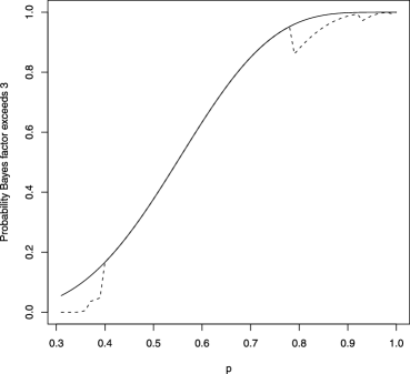
Figure 1: Probability that the Bayes factor exceeds 3 plotted against the data-generating parameter. The solid curve shows the probability of exceeding 3 for the UMPBT. The dashed curve displays this probability when the Bayes factor is calculated using the data-generating parameter.

A plot of the probability that $\mathrm{BF}_{10}$ exceeds $3$ as function of the true response rate $p$ appears in Figure 1. For comparison, also plotted in this figure (dashed curve) is the probability that $\mathrm{BF}_{10}$ exceeds 3 when $p_{1}$ is set to the data-generating parameter, that is, when $p_{1}=p_{t}$.

Figure 1 shows that the probability that $\mathrm{BF}_{10}$ exceeds 3 when calculated under the true alternative hypothesis is significantly smaller than it is under the UMPBT alternative for values of $p<0.4$ and for values of $p>0.78$. Indeed, for values of $p<0.334$, there is no chance that $\mathrm{BF}_{10}$ will exceed 3. This is so because $(0.334/0.30)^{x}$ remains less than 3.0 for all $x\leq 10$. The decrease in the probability that the Bayes factor exceeds 3 for large values of $p$ stems from the relatively small probability that these models assign to the observation of intermediate values of $x$. For example, when $p=0.8$, the probability of observing 6 out 10 successes is only 0.088, while the corresponding probability under $H_{0}$ is 0.037. Thus $\mathrm{BF}_{10}=2.39$, and the evidence in favor of the true success probability does not exceed 3. That is, the discontinuity in the dashed curve at $p\approx 0.7$ occurs because the Bayes factor for this test is not greater than 3 when $x=6$. Similarly, the other discontinuities in the dashed curve occur when the rejection region for the Bayesian test (i.e., values of $x$ for which the Bayes factor is greater than 3) excludes another immediate value of $x$. The dashed and solid curves agree for all Bayesian tests that produce Bayes factors that exceed 3 for all values of $x\geq 6$.

It is also interesting to note that the solid curve depicted in Figure 1 represents the power curve for an approximate 5% one-sided significance test of the null hypothesis that $p=0.3$ [note that $P_{0.3}(X\geq 6)=0.047$]. This rejection region for the 5% significance test also corresponds to the region for which the Bayes factor corresponding to the UMPBT($\gamma$) exceeds $\gamma$ for all values of $\gamma\in(2.36,6.82)$. If equal prior probabilities are assigned to $H_{0}$ and $H_{1}$, this suggests that a $p$-value of 0.05 for this test corresponds roughly to the assignment of a posterior probability between $(1.0/7.82,1.0/3.36)=(0.13,0.30)$ to the null hypothesis. This range of values for the posterior probability of the null hypothesis is in approximate agreement with values suggested by other authors, for example, Berger and Sellke (1987).

This example also indicates that a UMPBT can result in large type I errors if the threshold $\gamma$ is chosen to be too small. For instance, taking $\gamma=2$ in this example would lead to type I errors that were larger than 0.05.

It is important to note that the UMPBT does not provide a test that maximizes the expected weight of evidence, as equation (4) demonstrates. This point is illustrated in Figure 2, which depicts the expected weight of evidence obtained in favor of $H_{1}$ by a solid curve as the data-generating success probability is varied in

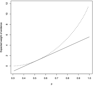
Figure 2: Expected weight of evidence produced by a $\operatorname{UMPBT}(\gamma)$ against a null hypothesis that $p_{0}=0.3$ when the sample size is $n=10$ (solid curve), versus the expected weight of evidence observed using the data-generating success probability at the alternative hypothesis (dashed curve). The data-generating parameter value is displayed on the horizontal axis.

$(0.3,1.0)$. For comparison, the dashed curve shows the expected weight of evidence obtained as a function of the true parameter value. As predicted by the inequality in (4), on average the UMPBT provides less evidence in favor of the true alternative hypothesis for all values of $p\in(0.3,1.0)$ except $p=0.525$, the UMPBT value.

3.2 Test of normal mean, $\sigma^{2}$ known

Suppose $x_{i}$, $i=1,\ldots,n$ are i.i.d. $N(\mu,\sigma^{2})$ with $\sigma^{2}$ known. The null hypothesis is $H_{0}\dvtx\mu=\mu_{0}$, and the alternative hypothesis is accepted if $\mathrm{BF}_{10}>\gamma$. Assuming that the alternative hypothesis takes the form $H_{1}\dvtx\mu=\mu_{1}$ in a one-sided test, it follows that

$$\log(\mathrm{BF}_{10})=\frac{n}{\sigma^{2}}\biggl{[}\bar{{\mathbf{x}}}(\mu_{1}-\mu_{0})+\frac{1}{2}\bigl{(}\mu_{0}^{2}-\mu_{1}^{2}\bigr{)}\biggr{]}.$$ (19)

If the data-generating parameter is $\mu_{t}$, the probability that $\mathrm{BF}_{10}$ is greater than $\gamma$ can be written as

$$\mathbf{P}_{\mu_{t}}\biggl{[}(\mu_{1}-\mu_{0})\bar{{\mathbf{x}}}>\frac{\sigma^{2}\log(\gamma)}{n}-\frac{1}{2}\bigl{(}\mu_{0}^{2}-\mu_{1}^{2}\bigr{)}\biggr{]}.$$ (20)

If $\mu_{1}>\mu_{0}$, then the UMPBT($\gamma$) value of $\mu_{1}$ satisfies

$$\mathop{\arg\min}_{\mu_{1}}\frac{\sigma^{2}\log(\gamma)}{n(\mu_{1}-\mu_{0})}+\frac{1}{2}(\mu_{0}+\mu_{1}).$$ (21)

Conversely, if $\mu_{1}<\mu_{0}$, then optimal value of $\mu_{1}$ satisfies

$$\mathop{\arg\min}_{\mu_{1}}\frac{\sigma^{2}\log(\gamma)}{n(\mu_{1}-\mu_{0})}+\frac{1}{2}(\mu_{0}+\mu_{1}).$$ (22)

It follows that the UMPBT($\gamma$) value for $\mu_{1}$ is given by

$$\mu_{1}=\mu_{0}\pm\sigma\sqrt{\frac{2\log\gamma}{n}},$$ (23)

depending on whether $\mu_{1}>\mu_{0}$ or $\mu_{1}<\mu_{0}$.

Figure 3 depicts the probability that the Bayes factor exceeds $\gamma=10$ when testing a null hypothesis that $\mu=0$ based on a single, standard normal observation (i.e., $n=1$, $\sigma^{2}=1$). In this case, the UMPBT(10) is obtained by taking $\mu_{1}=2.146$. For comparison, the probability that the Bayes factor exceeds 10 when the alternative is defined to be the data-generating parameter is depicted by the dashed curve in the plot.

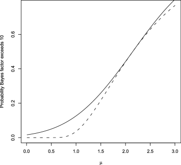
Figure 3: Probability that Bayes factor in favor of UMPBT alternative exceeds 10 when $\mu_{0}=0$ and $n=1$ (solid curve). The dashed curve displays this probability when the Bayes factor is calculated under the alternative hypothesis that $\mu_{1}$ equals the data-generating parameter (displayed on the horizontal axis).

UMPBTs can also be used to interpret the evidence obtained from classical UMPTs. In a classical one-sided test of a normal mean with known variance, the null hypothesis is rejected if

$$\bar{x}>\mu_{0}+z_{\alpha}\frac{\sigma}{\sqrt{n}},$$

where $\alpha$ is the level of the test designed to detect $\mu_{1}>\mu_{0}$. In the UMPBT, from (19)–(20) it follows that the null hypothesis is rejected if

$$\bar{x}>\frac{\sigma^{2}\log(\gamma)}{n(\mu_{1}-\mu_{0})}+\frac{1}{2}(\mu_{1}+\mu_{0}).$$

Setting $\mu_{1}=\mu_{0}+\sigma\sqrt{2\log(\gamma)/n}$ and equating the two rejection regions, it follows that the rejection regions for the two tests are identical if

$$\gamma=\exp\biggl{(}\frac{z_{\alpha}^{2}}{2}\biggr{)}.$$ (24)

For the case of normally distributed data, it follows that

$$\mu_{1}=\mu_{0}+\frac{\sigma}{\sqrt{n}}z_{\alpha},$$ (25)

which means that the alternative hypothesis places $\mu_{1}$ at the boundary of the UMPT rejection region.

The close connection between the UMPBT and UMPT for a normal mean makes it relatively straightforward to examine the relationship between the $p$-values reported from a classical test and either the Bayes factors or posterior probabilities obtained from a Bayesian test. For example, significance tests for normal means are often conducted at the 5% level. Given this threshold of evidence for rejection of the null hypothesis, the one-sided $\gamma$ threshold corresponding to the 5% significance test is 3.87, and the UMPBT alternative is $\mu_{1}=\mu_{0}+1.645\sigma/\sqrt{n}$. If we assume that equal prior

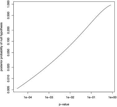
Figure 4: Correspondence between $p$-values and posterior model probabilities for a UMPBT test derived from a 5% test. This plot assumes equal prior probabilities were assigned to the null and alternative hypotheses. Note that both axes are displayed on the logarithmic scale.

probabilities are assigned to the null and alternative hypotheses, then a correspondence between $p$-values and posterior probabilities assigned to the null hypothesis is easy to establish. This correspondence is depicted in Figure 4. For instance, this figure shows that a $p$-value of 0.01 corresponds to the assignment of posterior probability 0.08 to the null hypothesis.

3.2.1 Evaluating evidence for the Higgs boson

On July 4, 2012, scientists at CERN made the following announcement:

We observe in our data clear signs of a new particle, at the level of 5 sigma, in the mass region around 126 gigaelectronvolts (GeV). (http://press.web.cern.ch/ press/PressReleases/Releases2012/PR17.12E.html).

In very simplified terms, the 5 sigma claim can be explained by fitting a model for a Poisson mean that had the following approximate form:

$$\mu(x)=\exp\bigl{(}a_{0}+a_{1}x+a_{2}x^{2}\bigr{)}+s\phi(x;m,w).$$

Here, $x$ denotes mass in GeV, $\{a_{i}\}$ denote nuisance parameters that model background events, $s$ denotes signal above background, $m$ denotes the mass of a new particle, $w$ denotes a convolution parameter and $\phi(x;m,w)$ denotes a Gaussian density centered on $m$ with standard deviation $w$ [Prosper (2012)]. Poisson events collected from a series of high energy experiments conducted in the Large Hadron Collider (LHC) at CERN provide the data to estimate the parameters in this stylized model. The background parameters $\{a_{i}\}$ are considered nuisance parameters. Interest, of course, focuses on testing whether $s>0$ at a mass location $m$. The null hypothesis is that $s=0$ for all $m$.

The accepted criterion for declaring the discovery of a new particle in the field of particle physics is the 5 sigma rule, which in this case requires that the estimate of $s$ be 5 standard errors from 0 (http://public.web.cern.ch/public/).

Calculation of a Bayes factor based on the original mass spectrum data is complicated by the fact that prior distributions for the nuisance parameters $\{a_{i}\}$, $m$, and $w$ are either not available or are not agreed upon. For this reason, it is more straightforward to compute a Bayes factor for these data based on the test statistic $z=\hat{s}/\operatorname{se}(\hat{s})$ where $\hat{s}$ denotes the maximum likelihood estimate of $s$ and $\operatorname{se}(\hat{s})$ its standard error [Johnson (2005, 2008)]. To perform this test, assume that under the null hypothesis $z$ has a standard normal distribution, and that under the alternative hypothesis $z$ has a normal distribution with mean $\mu$ and variance 1.

In this context, the 5 sigma rule for declaring a new particle discovery means that a new discovery can only be declared if the test statistic $z>5$. Using equation (24) to match the rejection region of the classical significance test to a UMPBT($\gamma$) implies that the corresponding evidence threshold is $\gamma=\exp(12.5)\approx 27\mbox{,}000$. In other words, a Bayes factor of approximately $\gamma=\exp(12.5)\approx 27\mbox{,}000$ corresponds to the 5 sigma rule required to accept the alternative hypothesis that a new particle has been found.

It follows from the discussion following equation (25) that the alternative hypothesis for the UMPBT alternative is $\mu_{1}=5$. This value is calculated under the assumption that the test statistic $z$ has a standard normal distribution under the null hypothesis [i.e., $\sigma=1$ and $n=1$ in (23)]. If the observed value of $z$ was exactly 5, then the Bayes factor in favor of a new particle would be approximately 27,000. If the observed value was, say 5.1, then the Bayes factor would be $\exp(-0.5[0.1^{2}-5.1^{2}])=44\mbox{,}000$. These values suggest very strong evidence in favor of a new particle, but perhaps not as much evidence as might be inferred by nonstatisticians by the report of a $p$-value of $3\times 10^{-7}$.

There are, of course, a number of important caveats that should be considered when interpreting the outcome of this analysis. This analysis assumes that an experiment with a fixed endpoint was conducted, and that the UMPBT value of the Poisson rate at 126 GeV was of physical significance. Referring to (23) and noting that the asymptotic standard error of $z$ decreases at rate $\sqrt{n}$, it follows that the UMPBT alternative hypothesis favored by this analysis is $O(n^{-1/2})$. For sufficiently large $n$, systematic errors in the estimation of the background rate could eventually lead to the rejection of the null hypothesis in favor of the hypothesis of a new particle. This is of particular concern if the high energy experiments were continued until a 5 sigma result was obtained. Further comments regarding this point appear in the discussion section.

3.3 Other one-parameter exponential family models

Table 2 provides the functions that must be minimized to obtain UMPBTs for a number of common exponential family models. The objective functions listed in this table correspond to the function

Table 2: Common one parameter exponential family models for which $\operatorname{UMPBT}(\gamma)$ exist

Model	Test	Objective function
Binomial	$p_{1}>p_{0}$	$\{\log(\gamma)-n\log[(1-p)/(1-p_{0})]\}(\log\{[p(1-p_{0})]/[(1-p)p_{0}]\})^{-1}$
Exponential	$\mu_{1}>\mu_{0}$	$\{\log(\gamma)+n[\log(\mu_{1})-\log(\mu_{0})]\}[1/\mu_{0}-1/\mu_{1}]^{-1}$
Neg. Bin.	$p_{1}>p_{0}$	$\{\log(\gamma)-r\log[(1-p_{1})/(1-p_{0})]\}[\log(p_{1})-\log(p_{0})]^{-1}$
Normal	$\sigma_{1}^{2}>\sigma_{0}^{2}$	$\{2\sigma_{1}^{2}\sigma_{0}^{2}(\log(\gamma)+\frac{n}{2}[\log(\sigma_{1}^{2})-\log(\sigma_{0}^{2})])\}[\sigma_{1}^{2}-\sigma_{0}^{2}]^{-1}$
Normal	$\mu_{1}>\mu_{0}$	$[\sigma^{2}\log(\gamma)](\mu_{1}-\mu_{0})^{-1}+\frac{1}{2}(\mu_{0}+\mu_{1})$
Poisson	$\mu_{1}>\mu_{0}$	$[\log(\gamma)+n(\mu_{1}-\mu_{0})][\log(\mu_{1})-\log(\mu_{0})]^{-1}$

$g_{\gamma}(\cdot,\cdot)$ specified in Lemma 1 with $v=1$. The negative binomial is parameterized by the fixed number of failures $r$ and random number of successes $x=0,1,\ldots$ observed before termination of sampling. The other models are parameterized so that $\mu$ and $p$ denote means and proportions, respectively, while $\sigma^{2}$ values refer to variances.

4 Extensions to other models

Like UMPTs, UMPBTs are most easily defined within one-parameter exponential family models. In unusual cases, UMPBTs can be defined for data modeled by vector-valued exponential family models, but in general such extensions appear to require stringent constraints on nuisance parameters.

One special case in which UMPBTs can be defined for a $d$-dimensional parameter ${\bolds\theta}$ occurs when the density of an observation can be expressed as

$$f(x\mid{\bolds\theta})=h(x)\exp\Biggl{[}\sum_{i=1}^{d}\eta_{i}({\bolds\theta})T_{i}(x)-A({\bolds\theta})\Biggr{]},$$ (26)

and all but one of the $\eta_{i}({\bolds\theta})$ are constrained to have identical values under both hypotheses. To understand how a UMPBT can be defined in this case, without loss of generality suppose that $\eta_{i}({\bolds\theta})$, $i=2,\ldots,d$ are constrained to have the same value under both the null and alternative hypotheses, and that the null and alternative hypotheses are defined by $H_{0}\dvtx\theta_{1}=\theta_{1,0}$ and $H_{1}\dvtx\theta_{1}>\theta_{1,0}$. For simplicity, suppose further that $\eta_{1}$ is a monotonically increasing function.

As in Lemma 1, consider first simple alternative hypotheses expressible as $H_{1}\dvtx\theta_{1}=\theta_{1,1}$. Let ${\bolds\theta}_{0}=(\theta_{1,0},\ldots,\theta_{d,0})^{\prime}$ and ${\bolds\theta}_{1}=(\theta_{1,1},\ldots,\theta_{d,1})^{\prime}$. It follows that the probability that the logarithm of the Bayes factor exceeds a threshold $\log(\gamma)$ can be expressed as

$$\mathbf{P}\bigl{[}\log(\mathrm{BF}_{10})>\log(\gamma)\bigr{]}$$

$$\qquad=\mathbf{P}\bigl{\{}\bigl{[}\eta_{1}(\theta_{1,1})-\eta_{1}(\theta_{1,0})\bigr{]}T_{1}({\mathbf{x}})-\bigl{[}A({\bolds\theta}_{1})-A({\bolds\theta}_{0})\bigr{]}>\log(\gamma)\bigr{\}}$$ (27)

$$\qquad=\mathbf{P}\biggl{[}T_{1}({\mathbf{x}})>\frac{\log(\gamma)+[A({\bolds\theta}_{1})-A({\bolds\theta}_{0})]}{[\eta_{1}(\theta_{1,1})-\eta_{1}(\theta_{1,0})]}\biggr{]}.$$

The probability in (4) is maximized by minimizing the right-hand side of the inequality. The extension to composite alternative hypotheses follows the logic described in inequalities (11)–(13), which shows that UMPBT($\gamma$) tests can be obtained in this setting by choosing the prior distribution of ${\bolds\theta}_{1}$ under the alternative hypotheses so that it concentrates its mass on the set

$$\mathop{\arg\min}_{\theta}\frac{\log(\gamma)+[A({\bolds\theta}_{1})-A({\bolds\theta}_{0})]}{[\eta_{1}(\theta_{1,1})-\eta_{1}(\theta_{1,0})]},$$ (28)

while maintaining the constraint that the values of $\eta_{i}({\bolds\theta})$ are equal under both hypotheses. Similar constructions apply if $\eta_{1}$ is monotonically decreasing, or if the alternative hypothesis specifies that $\theta_{1,0}<\theta_{0,0}$.

More practically useful extensions of UMPBTs can be obtained when it is possible to integrate out nuisance parameters in order to obtain a marginal density for the parameter of interest that falls within the class of exponential family of models. An important example of this type occurs in testing whether a regression coefficient in a linear model is zero.

4.1 Test of linear regression coefficient, $\sigma^{2}$ known

Suppose that

$$\mathbf{y}\sim N\bigl{(}\mathbf{X}{\bolds\beta},\sigma^{2}{\mathbf{I}}_{n}\bigr{)},$$ (29)

where $\sigma^{2}$ is known, $\mathbf{y}$ is an $n\times 1$ observation vector, $\mathbf{X}$ an $n\times p$ design matrix of full column rank and ${\bolds\beta}=(\beta_{1},\ldots,\beta_{p})^{\prime}$ denotes a $p\times 1$ regression parameter. The null hypothesis is defined as $H_{0}\dvtx\beta_{p}=0$. For concreteness, suppose that interest focuses on testing whether $\beta_{p}>0$, and that under both the null and alternative hypotheses, the prior density on the first $p-1$ components of ${\bolds\beta}$ is a multivariate normal distribution with mean vector ${\mathbf{0}}$ and covariance matrix $\sigma^{2}{\bolds\Sigma}$. Then the marginal density of $\mathbf{y}$ under $H_{0}$ is

$$m_{0}(\mathbf{y})=\bigl{(}2\pi\sigma^{2}\bigr{)}^{-n/2}|{\bolds\Sigma}|^{-{1}/{2}}|\mathbf{F}|^{-{1}/{2}}\exp\biggl{(}-\frac{R}{2\sigma^{2}}\biggr{)},$$ (30)

where

$$\quad\mathbf{F}=\mathbf{X}_{-p}^{\prime}\mathbf{X}_{-p}+{\bolds\Sigma}^{-1},\qquad{\mathbf{H}}=\mathbf{X}_{-p}\mathbf{F}^{-1}\mathbf{X}_{-p}^{\prime},\qquad R=\mathbf{y}^{\prime}({\mathbf{I}}_{n}-{\mathbf{H}})^{\prime}\mathbf{y},$$ (31)

and $\mathbf{X}_{-p}$ is the matrix consisting of the first $p-1$ columns of $\mathbf{X}$.

Let $\beta_{p*}$ denote the value of $\beta_{p}$ under the alternative hypothesis $H_{1}$ that defines the UMPBT($\gamma$), and let $\mathbf{x}_{p}$ denote the $p$th column of $\mathbf{X}$. Then the marginal density of $\mathbf{y}$ under $H_{1}$ is

$$\qquad m_{1}(\mathbf{y})=m_{0}(\mathbf{y})\times\exp\biggl{\{}-\frac{1}{2\sigma^{2}}\bigl{[}{\beta_{p*}}^{2}\mathbf{x}_{p}^{\prime}({\mathbf{I}}_{n}-{\mathbf{H}})\mathbf{x}_{p}-2{\beta_{p*}}\mathbf{x}_{p}^{\prime}({\mathbf{I}}_{n}-{\mathbf{H}})\mathbf{y}\bigr{]}\biggr{\}}.$$ (32)

It follows that the probability that the Bayes factor $\mathrm{BF}_{10}$ exceeds $\gamma$ can be expressed as

$$\mathbf{P}\biggl{[}\mathbf{x}_{p}^{\prime}(\mathbf{I}_{n}-{\mathbf{H}})\mathbf{y}>\frac{\sigma^{2}\log(\gamma)}{{\beta_{p*}}}+\frac{1}{2}{\beta_{p*}}\mathbf{x}_{p}^{\prime}({\mathbf{I}}_{n}-{\mathbf{H}})\mathbf{x}_{p}\biggr{]},$$ (33)

which is maximized by minimizing the right-hand side of the inequality. The UMPBT($\gamma$) is thus obtained by taking

$${\beta_{p*}}=\sqrt{\frac{2\sigma^{2}\log(\gamma)}{\mathbf{x}_{p}^{\prime}({\mathbf{I}}_{n}-{\mathbf{H}})\mathbf{x}_{p}}}.$$ (34)

The corresponding one-sided test of $\beta_{p}<0$ is obtained by reversing the sign of ${\beta_{p*}}$ in (34).

Because this expression for the UMPBT assumes that $\sigma^{2}$ is known, it is not of great practical significance by itself. However, this result may guide the specification of alternative models in, for example, model selection algorithms in which the priors on regression coefficients are specified conditionally on the value of $\sigma^{2}$. For example, the mode of the nonlocal priors described in Johnson and Rossell (2012) might be set to the UMPBT values after determining an appropriate value of $\gamma$ based on both the sample size $n$ and number of potential covariates $p$.

5 Approximations to UMPBTs using data-dependent alternatives

In some situations—most notably in linear models with unknown variances—data dependent alternative hypotheses can be defined to obtain tests that are approximately uniformly most powerful in maximizing the probability that a Bayes factor exceeds a threshold. This strategy is only attractive when the statistics used to define the alternative hypothesis are ancillary to the parameter of interest.

5.1 Test of normal mean, $\sigma^{2}$ unknown

Suppose that $x_{i}$, $i=1,\ldots,n$, are i.i.d. $N(\mu,\sigma^{2})$, that $\sigma^{2}$ is unknown and that the null hypothesis is $H_{0}\dvtx\mu=\mu_{0}$. For convenience, assume further that the prior distribution on $\sigma^{2}$ is an inverse gamma distribution with parameters $\alpha$ and $\lambda$ under both the null and alternative hypotheses.

To obtain an approximate UMPBT($\gamma$), first marginalize over $\sigma^{2}$ in both models. Noting that $(1+a/t)^{t}\rightarrow e^{a}$, it follows that the Bayes factor in favor of the alternative hypothesis satisfies

$$\mathrm{BF}_{10}({\mathbf{x}}) = \biggl{[}\frac{\sum_{i=1}^{n}(x_{i}-\mu_{0})^{2}+2\lambda}{\sum_{i=1}^{n}(x_{i}-\mu_{1})^{2}+2\lambda}\biggr{]}^{n/2+\alpha}$$ (35)

$$\approx \biggl{[}\frac{1+{(\bar{{\mathbf{x}}}-\mu_{0})^{2}}/{s^{2}}}{1+{(\bar{{\mathbf{x}}}-\mu_{1})^{2}}/{s^{2}}}\biggr{]}^{n/2+\alpha}$$ (36)

$$\approx \exp\biggl{\{}-\frac{n}{2s^{2}}\bigl{[}(\bar{{\mathbf{x}}}-\mu_{1})^{2}-(\bar{{\mathbf{x}}}-\mu_{0})^{2}\bigr{]}\biggr{\}},$$ (37)

where

$$s^{2}=\frac{\sum_{i=1}^{n}(x_{i}-\bar{{\mathbf{x}}})^{2}+2\lambda}{n+2\alpha}.$$ (38)

The expression for the Bayes factor in (37) reduces to (19) if $\sigma^{2}$ is replaced by $s^{2}$. This implies that an approximate, but data-dependent UMPBT alternative hypothesis can be specified by taking

$$\mu_{1}=\mu_{0}\pm s\sqrt{\frac{2\log\gamma}{n}},$$ (39)

depending on whether $\mu_{1}>\mu_{0}$ or $\mu_{1}<\mu_{0}$.

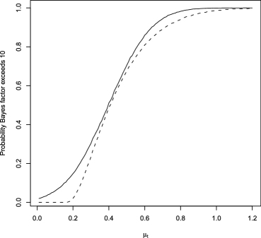
Figure 5: Probability that Bayes factor based on data-dependent, approximate UMPBT alternative exceeds 10 when $\mu_{0}=0$ and $n=30$ (solid curve). The dashed curve displays this probability when the Bayes factor is calculated under the alternative hypothesis that $\mu_{1}$ equals data-generating parameter (displayed on the horizontal axis) and $\sigma^{2}=1$ (the true value).

Figure 5 depicts the probability that the Bayes factor exceeds $\gamma=10$ when testing a null hypothesis that $\mu=0$ based on an independent sample of size $n=30$ normal observations with unit variance ($\sigma^{2}=1$) and using (39) to set the value of $\mu_{1}$ under the alternative hypothesis. For comparison, the probability that the Bayes factor exceeds 10 when the alternative is defined by taking $\sigma^{2}=1$ and $\mu_{1}$ to be the data-generating parameter is depicted by the dashed curve in the plot. Interestingly, the data-dependent, approximate UMPBT(10) provides a higher probability of producing a Bayes factor that exceeds 10 than do alternatives fixed at the data generating parameters.

5.2 Test of linear regression coefficient, $\sigma^{2}$ unknown

As final example, suppose that the sampling model of Section 4.1 holds, but assume now that the observational variance $\sigma^{2}$ is unknown and assumed under both hypotheses to be drawn from an inverse gamma distribution with parameters $\alpha$ and $\lambda$. Also assume that the prior distribution for the first $p-1$ components of ${\bolds\beta}$, given $\sigma^{2}$, is a multivariate normal distribution with mean ${\mathbf{0}}$ and covariance matrix $\sigma^{2}\Sigma$. As before, assume that $H_{0}\dvtx\beta_{p}=0$. Our goal is to determine a value ${\beta_{p*}}$ so that $H_{1}\dvtx\beta_{p}={\beta_{p*}}$ is the UMPBT($\gamma$) under the constraint that $\beta_{p}>0$.

Define $\mathbf{y}_{1}=\mathbf{y}-\mathbf{x}_{p}{\beta_{p*}}$ and let $\mathbf{y}_{0}=\mathbf{y}$. By integrating with respect to the prior densities on $\sigma^{2}$ and the first $p-1$ components of ${\bolds\beta}$, the marginal density of the data under hypothesis $i$, $i=0,1$ can be expressed as

$$m_{i}(\mathbf{y})=2^{\alpha}\pi^{-n/2}|\Sigma|^{-1/2}\frac{\lambda^{\alpha}}{\Gamma(\alpha)}\Gamma(n/2+\alpha)|{\mathbf{F}}|^{-1/2}R_{i}^{-n/2-\alpha},$$ (40)

where ${\mathbf{F}}$ is defined in (31), and

$$R_{i}=\mathbf{y}_{i}^{\prime}({\mathbf{I}}_{n}-{\mathbf{H}})\mathbf{y}_{i}+2\lambda.$$ (41)

It follows that the Bayes factor in favor of $H_{1}$ can be written as

$$\mathrm{BF}_{10} = \biggl{[}1+\frac{{\beta_{p*}}^{2}\mathbf{x}_{p}^{\prime}({\mathbf{I}}_{n}-{\mathbf{H}})\mathbf{x}_{p}-2{\beta_{p*}}\mathbf{x}_{p}^{\prime}({\mathbf{I}}_{n}-{\mathbf{H}})\mathbf{y}}{R_{0}}\biggr{]}^{-n/2-\alpha}$$ (42)

$$\approx \exp\biggl{\{}-\frac{1}{2s_{p}^{2}}\bigl{[}{\beta_{p*}}^{2}\mathbf{x}_{p}^{\prime}({\mathbf{I}}_{n}-{\mathbf{H}})\mathbf{x}_{p}-2{\beta_{p*}}\mathbf{x}_{p}^{\prime}({\mathbf{I}}_{n}-{\mathbf{H}})\mathbf{y}\bigr{]}\biggr{\}},$$ (43)

where

$$s_{p}^{2}=\frac{R_{0}}{n+2\alpha}.$$ (44)

The UMPBT($\gamma$) is defined from (43) according to

$$\quad\mathbf{P}(\mathrm{BF}_{10}>\gamma)=\mathbf{P}\biggl{[}\mathbf{x}_{p}^{\prime}({\mathbf{I}}_{n}-{\mathbf{H}})\mathbf{y}>\frac{s_{p}^{2}\log(\gamma)}{{\beta_{p*}}}+\frac{1}{2}{\beta_{p*}}\mathbf{x}_{p}^{\prime}({\mathbf{I}}_{n}-{\mathbf{H}})\mathbf{x}_{p}\biggr{]}.$$ (45)

Minimizing the right-hand side of the last inequality with respect to ${\beta_{p*}}$ results in

$${\beta_{p*}}=\sqrt{\frac{2s_{p}^{2}\log(\gamma)}{\mathbf{x}_{p}^{\prime}({\mathbf{I}}_{n}-{\mathbf{H}})\mathbf{x}_{p}}}.$$ (46)

This expression is consistent with the result obtained in the known variance case, but with $s_{p}^{2}$ substituted for $\sigma^{2}$.

6 Discussion

The major contributions of this paper are the definition of UMPBTs and the explicit description of UMPBTs for regular one-parameter exponential family models. The existence of UMPBTs for exponential family models is important because these tests represent the most common hypothesis tests conducted by practitioners. The availability of UMPBTs for these models means that these tests can be used to interpret test results in terms of Bayes factors and posterior model probabilities in a wide range of scientific settings. The utility of these tests is further enhanced by the connection between UMPBTs and UMPTs that have the same rejection region. This connection makes it trivial to simultaneously report both the $p$-value from a test and the corresponding Bayes factor.

The simultaneous report of default Bayes factors and $p$-values may play a pivotal role in dispelling the perception held by many scientists that a $p$-value of 0.05 corresponds to “significant” evidence against the null hypothesis. The preceding sections contain examples in which this level of significance favors the alternative hypothesis by odds of only 3 or 4 to 1. Because few researchers would regard such odds as strong evidence in favor of a new theory, the use of UMPBTs and the report of Bayes factors based upon them may lead to more realistic interpretations of evidence obtained from scientific studies.

The large sample properties of UMPBTs described in Section 2.1 deserve further comment. From Lemma 2, it follows that the expected weight of evidence in favor of a true null hypothesis in an exponential family model converges to $\log(\gamma)$ as the sample size $n$ tends to infinity. In other words, the evidence threshold $\gamma$ represents an approximate bound on the evidence that can be collected in favor of the null hypothesis. This implies that $\gamma$ must be increased with $n$ in order to obtain a consistent sequence of tests.

Several criteria might be used for selecting a value for $\gamma$ in large sample settings. One criterion can be inferred from the first statement of Lemma 2, where it is shown that the difference between the tested parameter’s value under the null and alternative hypotheses is proportional to $[\log(\gamma)/n]^{1/2}$. For this difference to be a constant—as it would be in a subjective Bayesian test—$\log(\gamma)$ must be proportional to $n$, or $\gamma=\exp(cn)$ for some $c>0$. This suggests that an appropriate value for $c$ might be determined by calibrating the weight of evidence against an accepted threshold/sample size combination. For example, if an evidence threshold of 4 were accepted as the standard threshold for tests conducted with a sample size of 100, then $c$ might be set to $\log(4)/100=0.0139$. This value of $c$ leads to an evidence threshold of $\gamma=16$ for sample sizes of 200, a threshold of 64 for sample sizes of 300, etc. From (24), the significance levels for corresponding $z$-tests would be 5%, 1% and 0.2%, respectively.

The requirement to increase $\gamma$ to achieve consistent tests in large samples also provides insight into the performance of standard frequentist and subjective Bayesian tests in large sample settings. The exponential growth rate of $\gamma$ required to maintain a fixed alternative hypothesis suggests that the weight of evidence should be considered against the backdrop of sample size, even in Bayesian tests. This is particularly important in goodness-of-fit testing where small deviations from a model may be tolerable. In such settings, even moderately large Bayes factors against the null hypotheses may not be scientifically important when they are based on very large sample sizes.

From a frequentist perspective, the use of UMPBTs in large sample settings can provide insight into the deviations from null hypotheses when they are (inevitably) detected. For instance, suppose that a one-sided 1% test has been conducted to determine if the mean of normal data is 0, and that the test is rejected with a $p$-value of 0.001 based on a sample size of 10,000. From (24), the implied evidence threshold for the test is $\gamma=15$, and the alternative hypothesis that has been implicitly tested with the UMPBT is that $\mu=0.023\sigma$. Based on the observation of $\bar{x}=0.031\sigma$, the Bayes factor in favor of this alternative is 88.5. Although there are strong odds against the null, the scientific importance of this outcome may be tempered by the fact that the alternative hypothesis that was supported against the null represents a standardized effect size of only 2.3%.

This article has focused on the specification of UMPBTs for one-sided alternatives. A simple extension of these tests to two-sided alternatives can be obtained by assuming that the alternative hypothesis is represented by two equally-weighted point masses located at the UMPBT values determined for one-sided tests. The Bayes factors for such tests can be written as

$$\mathbf{P}\biggl{[}\frac{0.5m_{l}({\mathbf{x}})+0.5m_{h}({\mathbf{x}})}{m_{0}({\mathbf{x}})}>\gamma\biggr{]},$$ (47)

where $m_{l}$ and $m_{h}$ denote marginal densities corresponding to one-sided UMPBTs. Letting $m_{*}({\mathbf{x}})=\max(m_{l}({\mathbf{x}}),m_{h}({\mathbf{x}}))$ for the data actually observed, and assuming that the favored marginal density dominates the other, it follows that

$$\mathbf{P}\biggl{[}\frac{0.5m_{l}({\mathbf{x}})+0.5m_{h}({\mathbf{x}})}{m_{0}({\mathbf{x}})}>\gamma\biggr{]}\approx\mathbf{P}\biggl{[}\frac{m_{*}({\mathbf{x}})}{m_{0}({\mathbf{x}})}>2\gamma\biggr{]}.$$ (48)

Thus, an approximate two-sided UMPBT($\gamma$) can be defined by specifying an alternative hypothesis that equally concentrates its mass on the two one-sided UMPBT($2\gamma$) tests.

Additional research is needed to identify classes of models and testing contexts for which UMPBTs can be defined. The UMPBTs described in this article primarily involve tests of point null hypotheses, or tests that can be reduced to a test of a point null hypothesis after marginalizing over nuisance parameters. Whether UMPBTs can be defined in more general settings remains an open question.

References

- Berger (2006) {barticle}[mr] \bauthor\bsnmBerger, \bfnmJames\binitsJ. (\byear2006). \btitleThe case for objective Bayesian analysis. \bjournalBayesian Anal. \bvolume1 \bpages385–402. \bidissn=1936-0975, mr=2221271 \bptokimsref \endbibitem
- Berger and Pericchi (1996) {barticle}[mr] \bauthor\bsnmBerger, \bfnmJames O.\binitsJ. O. and \bauthor\bsnmPericchi, \bfnmLuis R.\binitsL. R. (\byear1996). \btitleThe intrinsic Bayes factor for model selection and prediction. \bjournalJ. Amer. Statist. Assoc. \bvolume91 \bpages109–122. \biddoi=10.2307/2291387, issn=0162-1459, mr=1394065 \bptokimsref \endbibitem
- Berger and Sellke (1987) {barticle}[mr] \bauthor\bsnmBerger, \bfnmJames O.\binitsJ. O. and \bauthor\bsnmSellke, \bfnmThomas\binitsT. (\byear1987). \btitleTesting a point null hypothesis: Irreconcilability of values and evidence. \bjournalJ. Amer. Statist. Assoc. \bvolume82 \bpages112–122. \bptokimsref \endbibitem
- Berger and Wolpert (1984) {bbook}[mr] \bauthor\bsnmBerger, \bfnmJames O.\binitsJ. O. and \bauthor\bsnmWolpert, \bfnmRobert L.\binitsR. L. (\byear1984). \btitleThe Likelihood Principle. \bseriesInstitute of Mathematical Statistics Lecture Notes—Monograph Series \bvolume6. \bpublisherIMS, \blocationHayward, CA. \bidmr=0773665 \bptnotecheck year\bptokimsref \endbibitem
- Edwards, Lindman and Savage (1963) {barticle}[mr] \bauthor\bsnmEdwards, \bfnmW.\binitsW., \bauthor\bsnmLindman, \bfnmH.\binitsH. and \bauthor\bsnmSavage, \bfnmL.\binitsL. (\byear1963). \btitleBayesian statistical inference for psychological research. \bjournalPsychological Review \bvolume70 \bpages193–242. \bptokimsref \endbibitem
- Howson and Urbach (2005) {bbook}[auto:STB—2013/06/05—13:45:01] \bauthor\bsnmHowson, \bfnmC.\binitsC. and \bauthor\bsnmUrbach, \bfnmP.\binitsP. (\byear2005). \btitleScientific Reasoning: The Bayesian Approach, \bedition3rd ed. \bpublisherOpen Court, \blocationChicago, IL. \bptokimsref \endbibitem
- Jeffreys (1939) {bbook}[mr] \bauthor\bsnmJeffreys, \bfnmHarold\binitsH. (\byear1939). \btitleTheory of Probability. \bpublisherCambridge Univ. Press, \blocationCambridge. \bptokimsref \endbibitem
- Johnson (2005) {barticle}[mr] \bauthor\bsnmJohnson, \bfnmValen E.\binitsV. E. (\byear2005). \btitleBayes factors based on test statistics. \bjournalJ. R. Stat. Soc. Ser. B Stat. Methodol. \bvolume67 \bpages689–701. \biddoi=10.1111/j.1467-9868.2005.00521.x, issn=1369-7412, mr=2210687 \bptokimsref \endbibitem
- Johnson (2008) {barticle}[mr] \bauthor\bsnmJohnson, \bfnmValen E.\binitsV. E. (\byear2008). \btitleProperties of Bayes factors based on test statistics. \bjournalScand. J. Stat. \bvolume35 \bpages354–368. \biddoi=10.1111/j.1467-9469.2007.00576.x, issn=0303-6898, mr=2418746 \bptokimsref \endbibitem
- Johnson and Rossell (2010) {barticle}[mr] \bauthor\bsnmJohnson, \bfnmValen E.\binitsV. E. and \bauthor\bsnmRossell, \bfnmDavid\binitsD. (\byear2010). \btitleOn the use of non-local prior densities in Bayesian hypothesis tests. \bjournalJ. R. Stat. Soc. Ser. B Stat. Methodol. \bvolume72 \bpages143–170. \biddoi=10.1111/j.1467-9868.2009.00730.x, issn=1369-7412, mr=2830762 \bptokimsref \endbibitem
- Johnson and Rossell (2012) {barticle}[mr] \bauthor\bsnmJohnson, \bfnmValen E.\binitsV. E. and \bauthor\bsnmRossell, \bfnmDavid\binitsD. (\byear2012). \btitleBayesian model selection in high-dimensional settings. \bjournalJ. Amer. Statist. Assoc. \bvolume107 \bpages649–660. \biddoi=10.1080/01621459.2012.682536, issn=0162-1459, mr=2980074 \bptokimsref \endbibitem
- Lehmann and Romano (2005) {bbook}[mr] \bauthor\bsnmLehmann, \bfnmE. L.\binitsE. L. and \bauthor\bsnmRomano, \bfnmJoseph P.\binitsJ. P. (\byear2005). \btitleTesting Statistical Hypotheses, \bedition3rd ed. \bpublisherSpringer, \blocationNew York. \bidmr=2135927 \bptokimsref \endbibitem
- Lindley (1957) {barticle}[mr] \bauthor\bsnmLindley, \bfnmD.\binitsD. (\byear1957). \btitleA statistical paradox. \bjournalBiometrika \bvolume44 \bpages187–192. \bptokimsref \endbibitem
- Mayo and Spanos (2006) {barticle}[mr] \bauthor\bsnmMayo, \bfnmDeborah G.\binitsD. G. and \bauthor\bsnmSpanos, \bfnmAris\binitsA. (\byear2006). \btitleSevere testing as a basic concept in a Neyman–Pearson philosophy of induction. \bjournalBritish J. Philos. Sci. \bvolume57 \bpages323–357. \biddoi=10.1093/bjps/axl003, issn=0007-0882, mr=2249183 \bptokimsref \endbibitem
- Neyman and Pearson (1928) {barticle}[auto:STB—2013/06/05—13:45:01] \bauthor\bsnmNeyman, \bfnmJ.\binitsJ. and \bauthor\bsnmPearson, \bfnmE.\binitsE. (\byear1928). \btitleOn the use and interpretation of certain test criteria for purposes of statistical inference. \bjournalBiometrika \bvolume20A \bpages175–240. \bptokimsref \endbibitem
- Neyman and Pearson (1933) {barticle}[auto:STB—2013/06/05—13:45:01] \bauthor\bsnmNeyman, \bfnmJ.\binitsJ. and \bauthor\bsnmPearson, \bfnmE.\binitsE. (\byear1933). \btitleOn the problem of the most efficient tests of statistical hypotheses. \bjournalPhilos. Trans. R. Soc. Lond. Ser. A Math. Phys. Eng. Sci. \bvolume231 \bpages289–337. \bptokimsref \endbibitem
- O’Hagan (1995) {barticle}[mr] \bauthor\bsnmO’Hagan, \bfnmAnthony\binitsA. (\byear1995). \btitleFractional Bayes factors for model comparison. \bjournalJ. R. Stat. Soc. Ser. B Stat. Methodol. \bvolume57 \bpages99–118. \bptokimsref \endbibitem
- Pitman (1949) {bbook}[auto:STB—2013/06/05—13:45:01] \bauthor\bsnmPitman, \bfnmE.\binitsE. (\byear1949). \btitleLecture Notes on Nonparametric Statistical Inference. \bpublisherColumbia Univ., \blocationNew York. \bptokimsref \endbibitem
- Popper (1959) {bbook}[mr] \bauthor\bsnmPopper, \bfnmKarl R.\binitsK. R. (\byear1959). \btitleThe Logic of Scientific Discovery. \bpublisherHutchinson, \blocationLondon. \bidmr=0107593 \bptokimsref \endbibitem
- Prosper (2012) {bmisc}[auto:STB—2013/06/05—13:45:01] \borganizationProsper (\byear2012). \bhowpublishedPersonal communication to news@bayesian.org. \bptokimsref \endbibitem
- Robert, Chopin and Rousseau (2009) {barticle}[mr] \bauthor\bsnmRobert, \bfnmChristian P.\binitsC. P., \bauthor\bsnmChopin, \bfnmNicolas\binitsN. and \bauthor\bsnmRousseau, \bfnmJudith\binitsJ. (\byear2009). \btitleHarold Jeffreys’s theory of probability revisited. \bjournalStatist. Sci. \bvolume24 \bpages141–172. \biddoi=10.1214/09-STS284, issn=0883-4237, mr=2655841 \bptokimsref \endbibitem
- Rousseau (2007) {bincollection}[mr] \bauthor\bsnmRousseau, \bfnmJudith\binitsJ. (\byear2007). \btitleApproximating interval hypothesis: -values and Bayes factors. In \bbooktitleProceedings of the 2006 Valencia Conference (\beditorJ. Bernardo, \beditorM. Bayarri, \beditorJ. Berger, \beditorA. Dawid, \beditorD. Heckerman, \beditorA. Smith and \beditorM. West, eds.) \bpages1–27. \bpublisherOxford Univ. Press, \blocationOxford. \bptokimsref \endbibitem