On the distinguishability of histograms

Abstract

We consider an approach for testing the hypothesis that two realizations of the random variables in the form of histograms are taken from the same statistical population (i.e. two histograms are drawn from the same distribution). The approach is based on the notion “significance of deviation”. This approach allows to estimate the statistical difference between two histograms using multi-dimensional test statistics. The distinguishability of histograms is estimated with the help of the construction a number of clones (rehistograms) of the observed histograms.

1 Introduction

The test of the hypothesis that two histograms are drawn from the same distribution is an important goal in many applications. For example, this task exists for the monitoring of the experimental equipment in particle physics experiments. Let the experimental facility register the flow of events during two independent time intervals $[t_{1},t_{2}]$ and $[t_{3},t_{4}]$. Events from first time interval belong to statistical population of events $G_{1}$, events from second time interval belong to statistical population of events $G_{2}$. If facility (beam, detectors, data acquisition system, …) is in norm during both time intervals then the properties of events, registered in the facility during time interval $[t_{1},t_{2}]$, is the same as the properties of events, registered in the facility during time interval $[t_{3},t_{4}]$, i.e. $G_{1}=G_{2}$. If facility is out of norm during one of time intervals then the properties of events from statistical population $G_{1}$ differ from the properties of events from statistical population $G_{2}$, i.e. $G_{1}\neq G_{2}$. Often the monitoring of the experimental facility is performed with the use of the comparison of histograms, which reflect the properties of events.

Several approaches to formalize and resolve this problem were considered Porter . Recently, the comparison of weighted histograms was developed in paper Gagun . Usually, one-dimensional test statistics is used for the comparison of histograms.

In this paper we propose a method which allows to estimate the value of statistical difference between histograms with the use of several test statistics. As example, we consider the case of two test statistics, i.e. bidimensional test statistic.

2 Distribution of test statistics

Suppose, there are two histograms $hist_{1}$ and $hist_{2}$ (with $M$ bins in each histogram) as a result of the treatment of two independent samples of events. The first histogram is a set of 2M numbers

$hist_{1}:~{}\hat{n}_{11}\pm\hat{\sigma}_{11},\hat{n}_{21}\pm\hat{\sigma}_{21},\dots,\hat{n}_{M1}\pm\hat{\sigma}_{M1}$

and the second histogram, correspondingly, is a set of 2M numbers also

$hist_{2}:~{}\hat{n}_{12}\pm\hat{\sigma}_{12},\hat{n}_{22}\pm\hat{\sigma}_{22},\dots,\hat{n}_{M2}\pm\hat{\sigma}_{M2}$.

The volume of the first sample is $N_{1}$, i.e. $\displaystyle N_{1}\equiv\sum_{i=1}^{M}\hat{n}_{i1}$ and the volume of the second sample is $N_{2}$, i.e. $\displaystyle N_{2}\equiv\sum_{i=1}^{M}\hat{n}_{i2}$.

The most of methods for the histograms comparison use single test statistic as a “distance measure” for the consistency of two samples of events (see, for example Porter ).

We propose  to use test statistics $\hat{S}_{i},~{}~{}i=1,...,M$ (significances of deviation) for each bin for the histograms comparison. In the case of two observed histograms we consider the significance of deviation of the following type:

$$\hat{S}_{i}=\displaystyle\frac{\hat{n}_{i1}-K\hat{n}_{i2}}{\sqrt{\hat{\sigma}^{2}_{i1}+K^{2}\hat{\sigma}^{2}_{i2}}}\,.$$ (1)

Here $K=\displaystyle\frac{N_{1}}{N_{2}}$ is a coefficient of the normalization .

We use two first statistical moments $\displaystyle\bar{S}=\frac{\sum_{i=1}^{M}{\hat{S}_{i}}}{M}$, and $\displaystyle RMS=\sqrt{\frac{\sum_{i=1}^{M}{(\hat{S}_{i}-\bar{S})^{2}}}{M}}$. If condition $G_{1}=G_{2}$ ($G_{1}$ and $G_{2}$ are taken from the same flow of events) takes place then test statistics ($\hat{S}_{i},~{}~{}i=1,...,M$) obey the distribution which close to the standard normal distribution ${\cal N}(0,1)$. Correspondingly, the distribution of these test statistics is close to standard normal distribution too. In this case our bidimensional test statistic (“distance measure between two observed histograms”) $SRMS=(\bar{S},RMS)$ has a clear interpretation:

• if $SRMS=(0,0)$ then histograms are identical;

• if $SRMS\approx(0,1)$ then $G_{1}=G_{2}$ (if $\bar{S}\approx 0$ and $RMS<1$ then the overlapping exists between samples);

• if previous relations are not valid then $G_{1}\neq G_{2}$.

Note that the relation

$$RMS^{2}=\frac{\hat{\chi}^{2}}{M}-\bar{S}^{2}\,,$$ (2)

$$\hat{\chi}^{2}=\sum_{i=1}^{M}{\hat{S}_{i}^{2}}\,$$ (3)

shows that test statistic $\hat{\chi}^{2}$ is a combination of two test statistics $RMS$ and $\bar{S}$.

3 Rehistogramming

An accuracy of the estimation of statistical moments depends on the number of bins $M$ in histograms and observed values in bins. The accuracy can be estimated via Monte Carlo experiments. Two models of the statistical populations (pseudo populations) can be produced. Each of models represents one of the histograms.

In considered below example for each of histograms we produced 4999 clones by the Monte Carlo simulation for each bin $i$ of histogram $k$ using the normal distribution ${\cal N}(\hat{n}_{ik},\hat{\sigma}_{ik}),~{}i=1,...,M,~{}k=1,2$. As a result there are 5000 pairs of histograms for comparisons. The comparison is performed for each pair of histograms (5000 comparisons in our example). The distribution of the significances $\hat{S}_{i}$ is obtained as a result of each comparison. The moments of this distribution are calculated (in our case $\bar{S}$ and $RMS$). It allows to estimate the errors in determination of statistical moments.

This procedure can be named as “rehistogramming” in analogy with “resampling” in the bootstrap method Efron .

4 Distinguishability of histograms

The estimation of the distinguishability of histograms is performed with the use of hypotheses testing. “A probability of correct decision” ($1-\tilde{\kappa}$) about distinguishability of hypotheses NIM534 is used as a measure of the potential in distinguishing of two flows of events ($G_{1}$ and $G_{2}$) via comparison of histograms ($hist_{1}$ and $hist_{2}$).

It is a probability of the correct choice between two hypotheses “the histograms are produced by the treatment of events from the same event flow (the same statistical population)” or “the histograms are produced by the treatment of events from different event flows”. The value $1-\tilde{\kappa}$ characterizes the distinguishability of two histograms.

For $1-\tilde{\kappa}=1$ the distinguishability of histograms is 100%, i.e. histograms are produced by the treatment of events from different event flows.

For $1-\tilde{\kappa}=0$ we can’t distinguish the histograms, i.e. histograms are produced from the same event flow.

The probability of correct decision $1-\tilde{\kappa}$ is a function of type I error ($\alpha$) and the type II error ($\beta$) testing, namely 

$$1-\displaystyle\tilde{\kappa}=1-\frac{\alpha+\beta}{2-(\alpha+\beta)}\,.$$ (4)

5 Example

Let us consider a simple model with two histograms in which the random variable in each bin obeys the normal distribution $\displaystyle\varphi(x_{ik}|n_{ik})=\frac{1}{\sqrt{2\pi}\sigma_{ik}}~{}e^{-\frac{(x_{ik}-n_{ik})^{2}}{2\sigma^{2}_{ik}}}\,.$ Here the expected value in the bin $i$ is equal to $n_{ik}$ (in this example $n_{i1}=i$) and the variance $\sigma^{2}_{ik}$ is also equal to $n_{ik}$. $k$ is the histogram number ($k=1,2$). This model can be considered as the approximation of Poisson distribution by normal distribution.

All calculations, Monte Carlo experiments and histograms presentation in this paper are performed using ROOT code ROOT . Histograms are obtained from independent samples.

The example with histograms produced from the same events flow during unequal independent time ranges (Fig. 1) shows that the standard deviation of the distribution in the picture (right, down) can be used as an estimator of the statistical difference between histograms (this distribution is close to $\cal N$(0,1)).

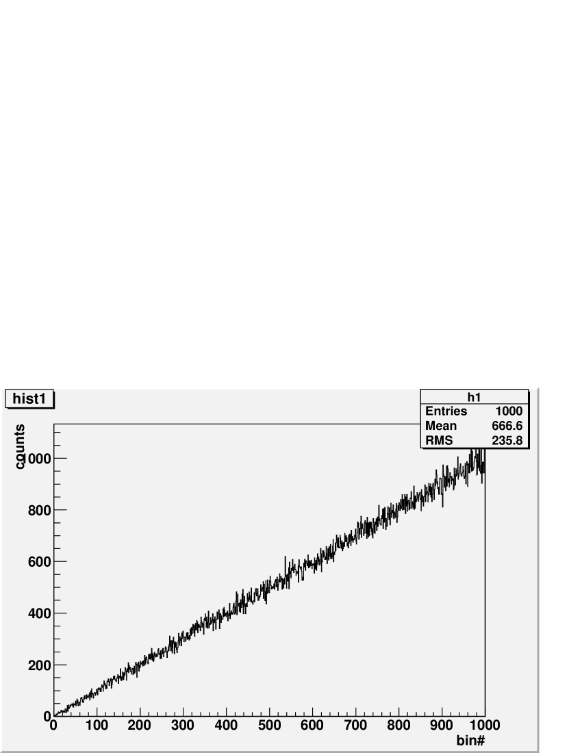
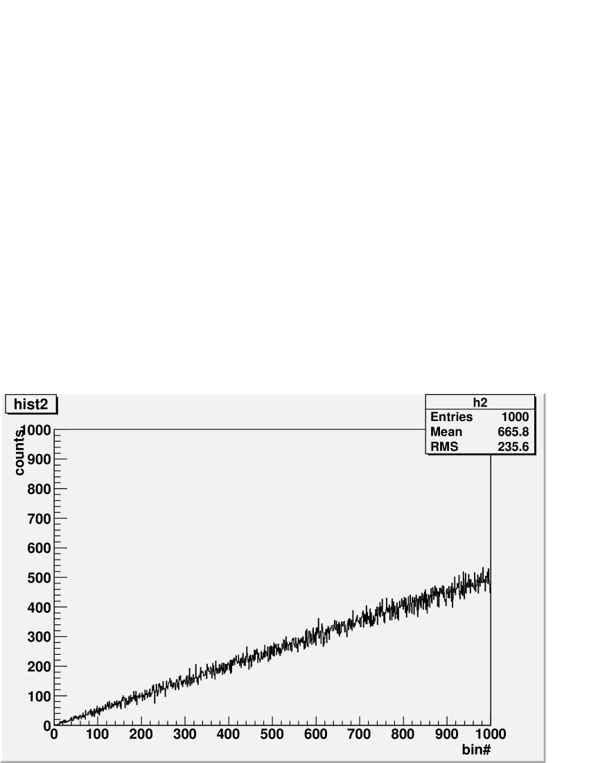
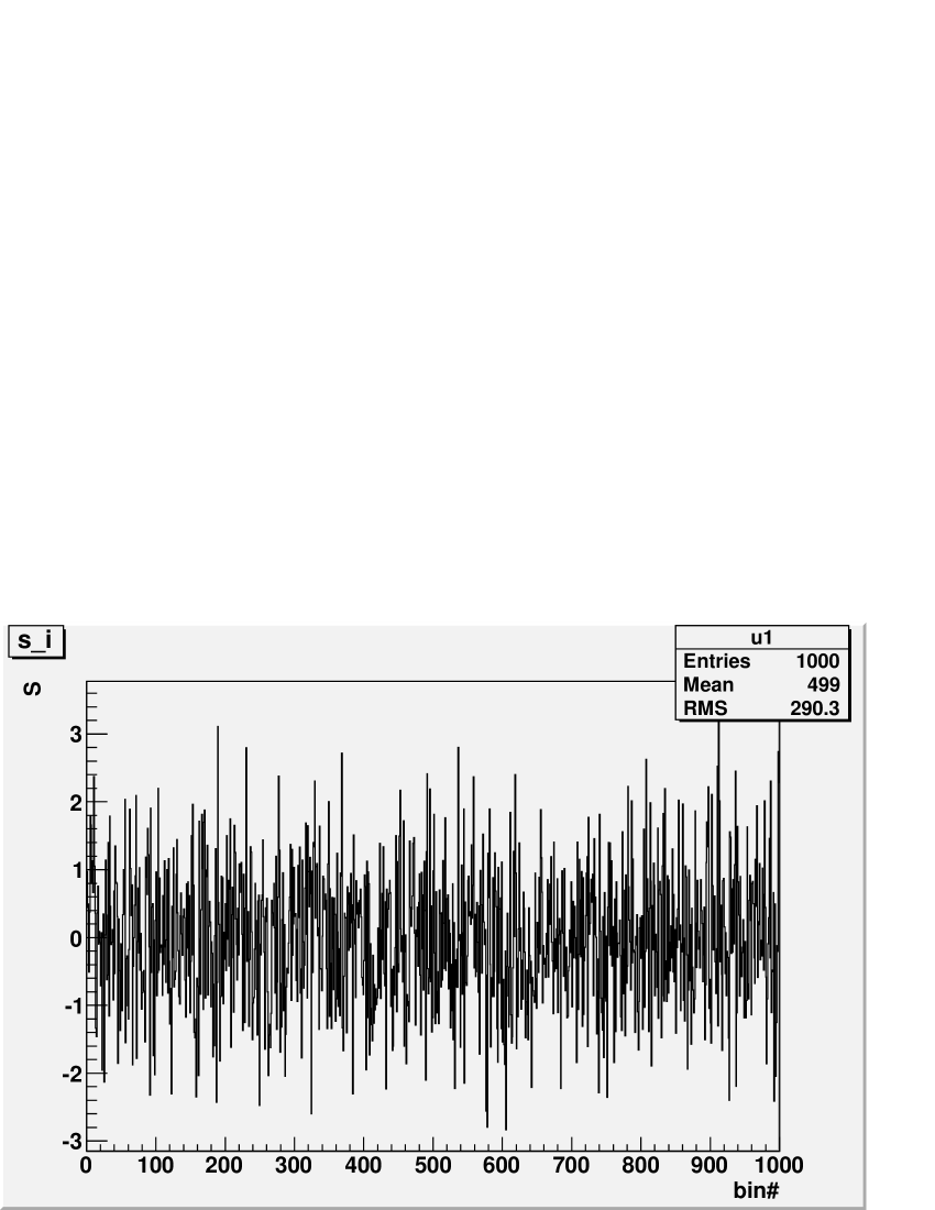
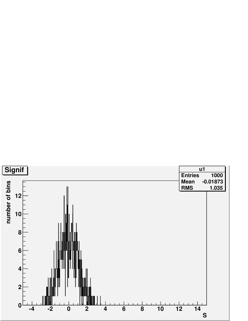
Figure 1: Triangle distributions in histograms ($M=1000$, $K=2$): the observed values $\hat{x}_{i1}$ in the first histogram (left, up), the observed values $\hat{x}_{i2}$ in the second histogram (right, up), observed normalized significances $\hat{S}_{i}$ bin-by-bin (left, down) and the distribution of observed normalized significances (right, down).

At first we consider the Case A (Fig. 2) when both histograms (hist1 and hist2) are obtained from the same statistical population. The distributions of test statistic $T_{\chi^{2}}=\sqrt{\frac{\hat{\chi}^{2}}{M}}$ and test statistic $RMS$ versus $\bar{S}$ are produced during 5000 comparisons of histograms (by the use of rehistogramming).

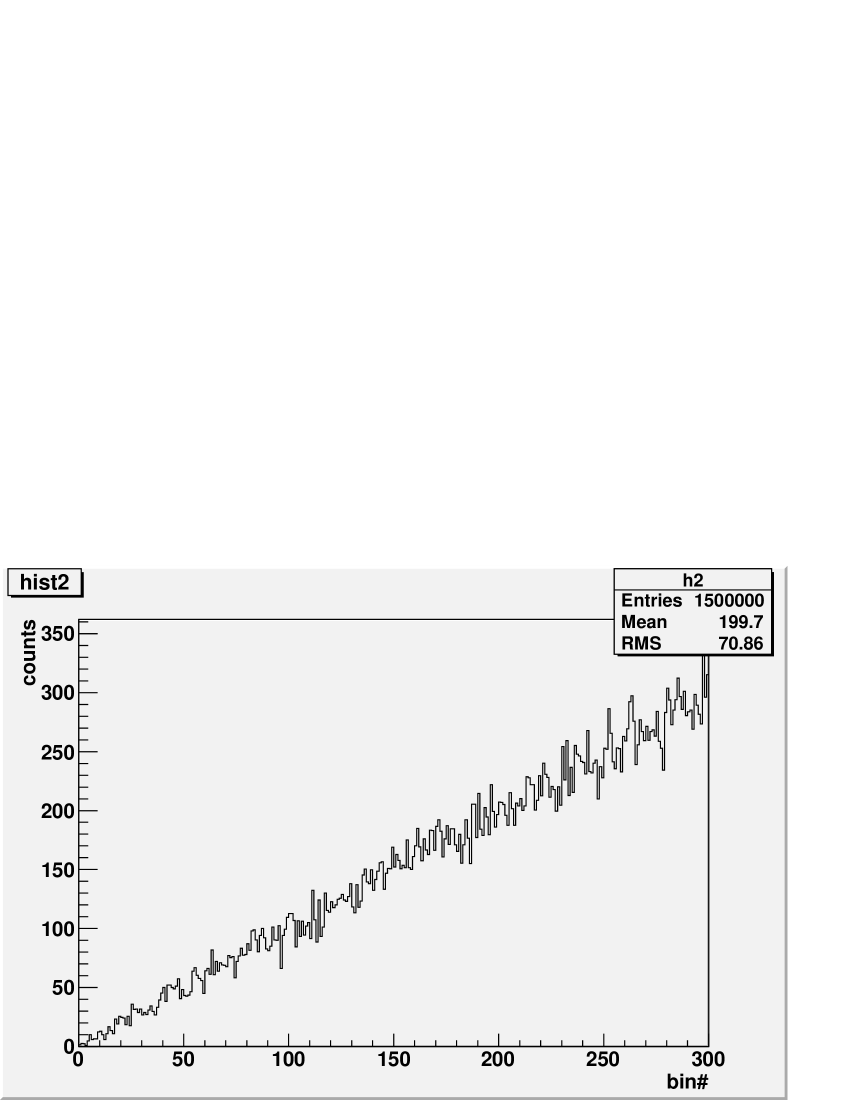
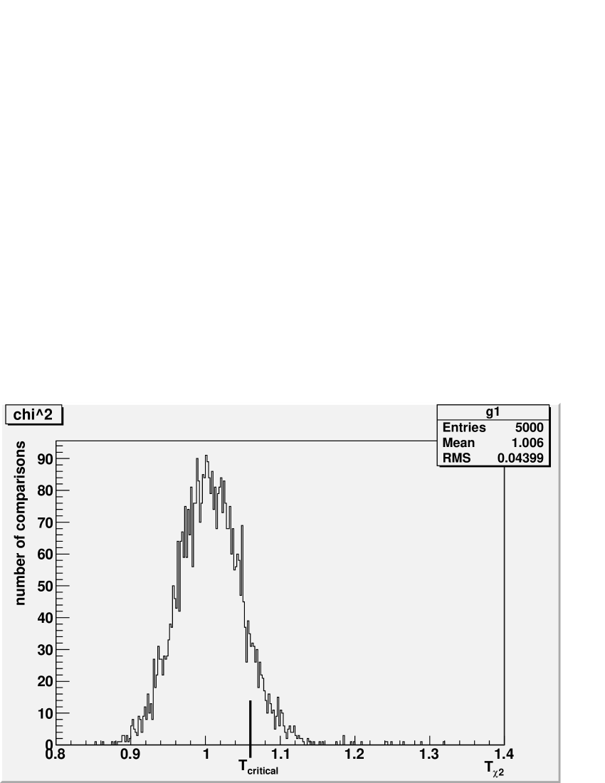
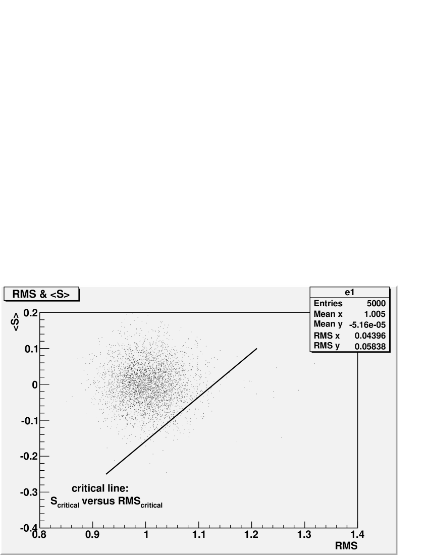
Figure 2: Case A: Upper histograms are input histograms (triangle distributions, M=300, K=1). Down histograms are $T_{\chi^{2}}$ (left) and $RMS$ & $\bar{S}$ (right) of the distribution of significances for 5000 comparisons for input histograms and their clones.

After that, the content of second histogram (hist2) was changed (Case B), namely, the expected content of left bin of histogram was increased from $n_{12}=1.0$ up to $n_{12}=8.5$, the expected content of right bin of histogram was decreased from $n_{M2}=300.0$ up to $n_{M2}=292.5$, the expected content of other bins was changed to conserve linear dependence between contents in bins. The result of the rehistogramming for the Case B is shown in Fig. 3. One can see that distributions of test statistic $T_{\chi^{2}}=\sqrt{\frac{\hat{\chi}^{2}}{M}}$ and test statistic $RMS$ versus $\bar{S}$ are shifted.

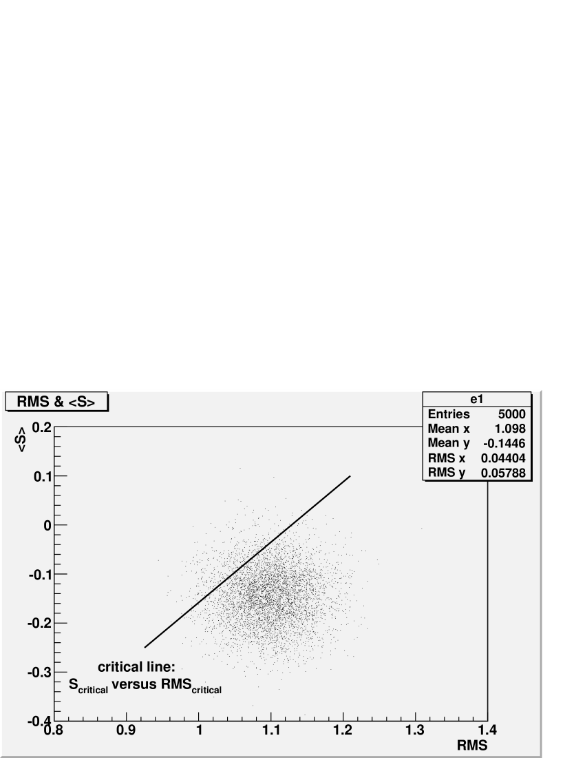
Figure 3: Case B: Upper histograms are input histograms (the triangle distribution (left) and the trapezoidal distribution (right), M=300, K=1). Down histograms are $T_{\chi^{2}}$ (left) and $RMS$ & $\bar{S}$ (right) of the distribution of significances for 5000 comparisons for input histograms and their clones.

The probability of correct decision as a measure for distinguishability of two histograms is determined by the comparison of distributions for the Case A and corresponding distributions for the Case B. The critical value $T_{critical}=1.06$ is used for comparison of one-dimensional $T_{\chi^{2}}$ distributions. The critical line $(S_{critical}=1.2\cdot RMS_{critical}-1.36)$ is used for comparison of two-dimensional $RMS\&\bar{S}$ distributions. The results are presented in Tab. 1.

For $\chi^{2}$ method the probability of the correct decision ($1-\kappa$) about the Case realization (A or B) is equal to 87.26%. For the other method the probability of the correct decision ($1-\kappa$) about the Case realization (A or B) is equal to 93.88%. One can see that the method, which uses $RMS$ and $\bar{S}$, gives better distinguishability of histograms than the $\chi^{2}$ method. Note that we use only two moments of the significance distributions (the first initial moment ($\bar{S}$) and the square root from the second central moment ($RMS$)) for the estimation of distinguishability of histograms.

6 Conclusions

The considered approach allows to perform the comparison of histograms in more details than methods which use only one test statistics. Our method can be used in tasks of monitoring of the equipment during experiments.

The main items of the consideration are

• the normalized significance of deviation provides us the distribution which is close to $\cal N$(0,1) if $G_{1}=G_{2}$;

• the rehistogramming provides us the tool for an estimation of the accuracy in the determination of statistical moments and, correspondingly, for testing the hypothesis about distinguishability of histograms;

• the probability of correct decision gives us the estimator of the decision quality.

Distribution of $T_{\chi^{2}}$			Distribution of $RMS\&\bar{S}$
	In reality			In reality
Accepted	Case A	Case B	Accepted	Case A	Case B
Case A	4543	673	Case A	4843	456
Case B	457	4327	Case B	121	4544
$1-\kappa$	$\alpha$	$\beta$	$1-\kappa$	$\alpha$	$\beta$
0.8726	0.0914	0.1346	0.9388	0.0242	0.0912

Table 1: The quality of the hypothesis testing about distinguishability of two different histograms for two methods of comparison histograms.