Edge theories in Projected Entangled Pair State models

Abstract

We study the edge physics of gapped quantum systems in the framework of Projected Entangled Pair State (PEPS) models. We show that the effective low-energy model for any region acts on the entanglement degrees of freedom at the boundary, corresponding to physical excitations located at the edge. This allows us to determine the edge Hamiltonian in the vicinity of PEPS models, and we demonstrate that by choosing the appropriate bulk perturbation, the edge Hamiltonian can exhibit a rich phase diagram and phase transitions. While for models in the trivial phase any Hamiltonian can be realized at the edge, we show that for topological models, the edge Hamiltonian is constrained by the topological order in the bulk which can e.g. protect a ferromagnetic Ising chain at the edge against spontaneous symmetry breaking.

The edge of strongly correlated quantum systems can display very intriguing phenomena. For instance, in two-dimensional (2D) quantum Hall systems the low energy behavior can be described in terms of chiral modes which live at the edge of the material Wen (1990, 1995). Interestingly, these edge modes cannot be described by a conventional one-dimensional (1D) theory, and their properties are dictated by the presence of a topologically ordered bulk.

In this Letter, we study the low-energy physics for a class of spin systems on 2D lattices. We show that the Hilbert space of the effective low-energy theory can be identified with the entanglement degrees of freedom which live at the edge of the system. This allows us to construct 1D edge Hamiltonians which describe the low-energy physics of the system, and investigate how they change under perturbations in the bulk. We find that bulk perturbations can induce phase transitions at the boundary, and explicitly investigate one particular example where we find a rich phase diagram with gapped, gapless, and symmetry-broken phases at the boundary. We also study the effect of topological order in the bulk and find that it induces constraints on the edge Hamiltonian which cannot occur in conventional 1D spin systems, a direct consequence of the topological protection Gu and Wen ; Chen et al. (2012); for instance, we give a model based on the Toric Code Kitaev (2003) whose edge Hamiltonian is an Ising chain, but which is protected against spontaneous symmetry breaking by the topological properties of the bulk.

We restrict our attention to Projected Entangled Pair State (PEPS) models, and perturbations thereof. PEPS models consist of a Hamiltonian $H$ together with its ground space which are both derived from a single tensor which describes the entanglement structure of the system locally Affleck et al. (1988); Verstraete and Cirac (2004); Perez-Garcia et al. (2008); Schuch et al. (2010). We focus on models where $H=\sum h$ is translational invariant, i.e., a sum of identical local terms, and gapped for periodic boundaries (PBC). Many paradigmatic models such as the AKLT model Affleck et al. (1988), topologically ordered systems Verstraete et al. (2006); Buerschaper et al. (2009); Gu et al. (2009), or Resonating Valence Bond (RVB) states Verstraete et al. (2006); Schuch et al. (2012) are PEPS models; and we will illustrate our results with particular perturbations of these models.

We start by introducing PEPS models. For simplicity, we restrict to square lattices and translationally invariant systems. The central object is a five-index tensor $A^{i}_{\mu_{1},\mu_{2},\mu_{3},\mu_{4}}$, with physical index $i=1,\dots,d$ and virtual indices $\mu_{k}=1,\dots,D$. For a given region $R$, these tensors are arranged on a 2D grid as shown in Fig. 1(a). Adjacent virtual indices $\mu_{k}$ in the bulk are contracted (i.e., identified and summed over), while the “open” virtual indices at the boundary are set to $\bm{\alpha}\equiv(\alpha_{1},\dots,\alpha_{|\partial R|})$. One remains with a tensor $c_{i_{1},\dots,i_{N}}(\bm{\alpha})$, which describes a physical state (a PEPS) $|\Phi_{\bm{\alpha}}\rangle=\sum c_{i_{1},\dots,i_{N}}(\bm{\alpha})|i_{1},\dots,i_{N}\rangle$. This defines a linear map $\mathcal{X}:|\bm{\alpha})\mapsto\mathcal{X}|\bm{\alpha})\equiv|\Phi_{\bm{\alpha}}\rangle$ between states $|\bm{\alpha})\in(\mathbb{C}^{D})^{\otimes|\partial R|}$ on the boundary and the subspace $\mathcal{S}\equiv\mathrm{span}\,\big{\{}|\Phi_{\bm{\alpha}}\rangle\big{\}}\subset(\mathbb{C}^{d})^{\otimes|R|}$ of physical states. [We use $|\,\cdot\,)$ to denote states on the virtual boundary.] Note that equivalently, one can construct $|\Phi_{\bm{\alpha}}\rangle$ by placing virtual bonds $\sum_{\mu=1}^{D}|\mu,\mu)$ with bond dimension $D$ along the edges, the state $|\bm{\alpha})$ at the boundary, and applying the linear map described by $A$ at every site Verstraete and Cirac (2004).

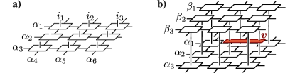
Figure 1: a) Construction of a PEPS by contracting local tensors. PEPS give a map from the boundary indices $(\alpha_{1},\alpha_{2},\dots)$ to the bulk indices $(i_{1},i_{2},\dots)$. b) Using this map, any bulk Hamiltonian $v$ naturally induces a Hamiltonian on the boundary by sandwiching $v$ in between the PEPS. Note that the boundary degrees of freedom still need to be orthogonalized.

Having defined the PEPS states $|\Phi_{\bm{\alpha}}\rangle$ and the PEPS subspace $\mathcal{S}=\mathrm{span}\,\{|\Phi_{\bm{\alpha}}\rangle\}$, let us now turn towards Hamiltonians for PEPS models. A parent Hamiltonian is a local Hamiltonian $H=\sum h$ such that for any (sufficiently large) region $R$ (i) $h\geq 0$, and $H|\Phi_{\bm{\alpha}}\rangle=0\ \forall\,|\bm{\alpha})$, i.e., $H$ is frustration free and all states in $\mathcal{S}$ are ground states of $H$; and (ii) all ground states of $H$ are of the form $|\Phi_{\bm{\alpha}}\rangle$, $\mathrm{ker}\,H=\mathcal{S}$; this is known as the intersection property Affleck et al. (1988); Perez-Garcia et al. (2008); Schuch et al. (2010). Given a PEPS, a parent Hamiltonian can be constructed by choosing $\ker h=\mathcal{S}$ for some small region (e.g. as a projector), where appropriate conditions on $A$ (which hold for generic tensors) ensure the intersection property Perez-Garcia et al. (2008); Schuch et al. (2010); since $\mathrm{rank}\,\mathcal{S}\leq D^{|\partial R|}$ for large enough $R$, such $h$ always exist. The paradigmatic example of a PEPS model is the AKLT model Affleck et al. (1988), which is constructed by placing spin-$\tfrac{1}{2}$ singlet bonds along the edges and subsequently projecting onto the maximal spin subspace ($S=2$ on the square lattice); the parent Hamiltonian is obtained by observing that for any two adjacent sites, the total spin cannot be $S=4$, and choosing $h=\Pi_{S=4}$ (the projector onto the $S=4$ subspace).

We now start from a PEPS model, specified by $H=\sum h$ and a tensor $A$ characterizing its ground space $\mathcal{S}$, with a gap $\Delta$ above the ground space, and consider an arbitrary perturbation to this model, $H^{\prime}=H+V=\sum(h+v)$, where $\|V\|\ll\|H\|$. What is the low-energy physics of the perturbed model $H+V$? In leading order, it is given by the effective Hamiltonian $H_{\mathrm{eff}}=\Pi_{\mathcal{S}}V\Pi_{\mathcal{S}}$, where $\Pi_{\mathcal{S}}$ is the projector onto the ground space $\mathcal{S}$ of $H$, i.e., the low-energy physics takes place in the subspace $\mathcal{S}$. Since $\mathcal{S}=\mathrm{span}\,\{|\Phi_{\bm{\alpha}}\rangle\}$, this implies that the states which describe the low-energy physics are in one-to-one correspondence with states $|\bm{\alpha})$ on the virtual edge (via the inverse of the map $\mathcal{X}$), and thus, the low-energy states exhibit a 1D structure which is associated to the edge. Even more, if the system does not break local symmetries (more technically, if it satisfies the weak LTQO condition Michalakis and Pytel (2011); Cirac et al. (2013)), these states are exponentially localized at the edge, i.e., different $|\Phi_{\bm{\alpha}}\rangle$ do not differ in the bulk. Together, this shows that the low-energy Hamiltonian $H_{\mathrm{eff}}$ can indeed be understood as a 1D Hamiltonian acting on degrees of freedom localized at the edge.

Let us now show how to determine the 1D model which describes the effective low-energy physics. To this end, we work in the 1D basis $|\bm{\alpha})$ which lives on the virtual edge indices. There, the perturbation induces a term $(\bm{\alpha}^{\prime}|\mathcal{M}|\bm{\alpha})=\langle\Phi_{\bm{\alpha}^{\prime}}|V|\Phi_{\bm{\alpha}}\rangle$; this is, $\mathcal{M}$ is obtained by sandwiching the Hamiltonian between a ket PEPS and a bra PEPS, as shown in Fig. 1b. However, the map $\mathcal{X}:|\bm{\alpha})\mapsto|\Phi_{\bm{\alpha}}\rangle$ does not preserve orthogonality, and thus, in order to obtain an edge Hamiltonian $\mathcal{H}$ which is isomorphic to $H_{\mathrm{eff}}$, we need to orthogonalize $\mathcal{M}$, $\mathcal{H}=\mathcal{P}^{-1}\mathcal{M}\mathcal{P}^{-1}$, where $\mathcal{P}=\sqrt{\mathcal{Q}}$, $(\bm{\alpha}^{\prime}|\mathcal{Q}|\bm{\alpha})=\langle\Phi_{\bm{\alpha}^{\prime}}|\Phi_{\bm{\alpha}}\rangle$. Put more formally, we can write $\mathcal{X}=\mathcal{W}\mathcal{P}$, with $\mathcal{P}$ a positive map acting on the virtual indices and $\mathcal{W}$ an isometry from the virtual to the physical system; then, the edge Hamiltonian is $\mathcal{H}=\mathcal{W}^{\dagger}V\mathcal{W}=\mathcal{P}^{-1}\mathcal{X}^{\dagger}V\mathcal{X}\mathcal{P}^{-1}$ (where $\mathcal{X}^{\dagger}V\mathcal{X}$ is the tensor network in Fig. 1b), and thus indeed isomorphic to $H_{\mathrm{eff}}$.

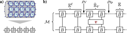
Figure 2: a) By blocking columns, a PEPS on a cylinder can be mapped to an MPS. b) Computation of the edge Hamiltonian on a long cylinder, cf. text.

In order to numerically study edge Hamiltonians, we restrict to translationally invariant PEPS on infinite cylinders. In this case, we can block columns and treat the system as an effective 1D PEPS, i.e., a Matrix Product State (MPS), see Fig. 2a. The central object encoding the behavior of the system is the transfer operator $\mathbb{E}_{O}=\sum_{ij}\langle j|O|i\rangle B^{i}\otimes\bar{B}^{j}$, where $i$ and $j$ ($B$, $O$) are blocked indices (tensors, operators) for one column. We first focus on systems where $\mathbb{E}\equiv\mathbb{E}_{\openone}$ has a non-degenerate largest eigenvalue with a gap below (this corresponds to a unique ground state with PBC); we assume the largest eigenvalue to be normalized to $1$. One first determines the fixed point $\rho_{\mathrm{fp}}$ of $\mathbb{E}$. Second, one applies $\rho_{V}=\tilde{\mathbb{E}}_{V}\cdot\rho_{\mathrm{fp}}$, where $\tilde{\mathbb{E}}_{V}$ is a transfer operator containing one unit cell of $V$ [e.g. two columns for a nearest neighbor (NN) Hamiltonian]. Finally, one iteratively computes the fixed point $\mathcal{M}=(\openone+\mathbb{E}+\mathbb{E}^{2}+\dots)\rho_{V}$. Now, to obtain $\mathcal{H}$ one needs to orthogonalize with $\mathcal{P}=\sqrt{\rho_{\mathrm{fp}}}$, i.e., the edge Hamiltonian $\mathcal{H}$ is obtained as $\mathcal{H}=\rho_{\mathrm{fp}}^{-1/2}\mathcal{M}\rho_{\mathrm{fp}}^{-1/2}$; the invertibility of $\rho_{\mathrm{fp}}$ follows from the uniqueness of the fixed point of $\mathbb{E}$ Perez-Garcia et al. (2007). The procedure is illustrated in Fig. 2b; note that $\mathbb{E}$ is evaluated as a Matrix Product Operator and thus, we are limited by the dimension of its eigenvectors rather than that of $\mathbb{E}$ itself. Note also that the dynamics on the two edges is independent; had we considered a finite cylinder instead, the dynamics of the two boundaries would be weakly coupled, with the length scale set by the gap of $\mathbb{E}$.

An essential point to note about the structure of the edge Hamiltonian is that it inherits all (on-site) symmetries shared by the PEPS and the bulk perturbation: Any symmetry action on a PEPS can be moved from the physical index to an action of the same symmetry on the virtual indices Perez-Garcia et al. (2010), and thus ultimately any symmetry of the state shared by $V$ shows up as a symmetry at the boundary degrees of freedom and thus in $\mathcal{H}$; the argument generalizes to other symmetries such as reflection or time reversal.

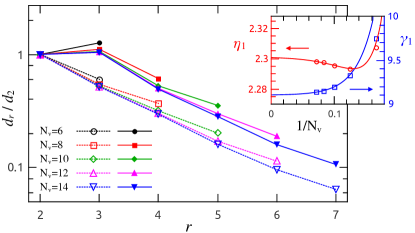
Figure 3: Edge Hamiltonian for the perturbed AKLT model: Exponential decay of the interaction strength of range-$r$ terms, $d_{r}$, with distance, for different $N_{v}$, for $\mathcal{H}_{J}$ (solid lines) and $\mathcal{H}_{g}$ (dotted lines). Inset: Finite size scaling of $\eta_{1}$ (red circles) and $\gamma_{1}$ (blue squares) vs. $1/N_{v}$.

As an example, we have studied the edge Hamiltonian $\mathcal{H}$ of the square lattice AKLT model on an infinitely long cylinder of diameter $N_{v}$, for the class of $\mathrm{U(1)}$ invariant perturbations

$$V=\sum_{\left\langle ij\right\rangle}\left[J\,\bm{S}_{i}\cdot\bm{S}_{j}+gS_{i}^{z}S_{j}^{z}\right]+h\sum_{i}S_{i}^{z}\ ,$$ (1)

i.e., an anisotropic Heisenberg Hamiltonian with a magnetic field. Since $\mathcal{H}$ is linear in $V$, we can write $\mathcal{H}=J\mathcal{H}_{J}+g\mathcal{H}_{g}+h\mathcal{H}_{h}$; as $D=2$, the $\mathcal{H}_{\bullet}$ ($\bullet=J,g,h$) are spin-$\tfrac{1}{2}$ Hamiltonians with translational and $\mathrm{U(1)}$ symmetry [$\mathrm{SU}(2)$ for $\mathcal{H}_{J}$]. Note that due to symmetry, $\mathcal{H}_{J}$ is completely determined by $\mathcal{H}_{g}$.

First, let us see whether the $\mathcal{H}_{\bullet}$ are sums of local terms. To this end, we decompose $\mathcal{H}_{\bullet}$ in a Pauli basis, and denote by $d_{r}$ the total weight of all terms which span $r$ contiguous sites (see Cirac et al. (2011); Schuch et al. (2013)). Fig. 3 shows the result for $\mathcal{H}_{J}$ and $\mathcal{H}_{g}$: In both cases $d_{r}$ decays exponentially with $r$, indicating that the edge Hamiltonian is approximately local. Let us now have a closer look at the individual terms. For $\mathcal{H}_{J}$, symmetries restrict the possible two- and three-body terms to Heisenberg couplings, which—following Fig. 3—are the dominating terms. More generally, we find

$$\mathcal{H}_{J}\approx\sum_{\ell\geq 1}\eta_{\ell}\sum_{i}\bm{S}_{i}\cdot\bm{S}_{i+\ell}$$ (2)

where $\eta_{1}\approx 2.298$ and $\eta_{2}\approx-2.394$, larger $\eta_{\ell}$ decay exponentially, and many-body terms are strongly supressed. Remarkably, the NN and next-nearest neighbor (NNN) Heisenberg terms in $\mathcal{H}_{J}$ have essentially the same strength, but opposite sign (this staggering repeats in the—exponentially decaying—longer-range $\eta_{\ell}$ and arises from the alternating parity of singlets connecting the bulk perturbation to the boundary). Adding an $S^{z}_{i}S^{z}_{j}$ anisotropy in the bulk leads to an anisotropy at the edge with a similarly staggered structure and a renormalized Heisenberg term,

$$\mathcal{H}_{g}\approx\sum_{\ell\geq 1}\left[\gamma_{\ell}\sum_{i}S_{i}^{z}S_{i+\ell}^{z}+\frac{\eta_{\ell}-\gamma_{\ell}}{3}\sum_{i}\bm{S}_{i}\cdot\bm{S}_{i+\ell}\right]$$ (3)

but with supressed NNN amplitudes $\gamma_{1}\approx 9.137$, $\gamma_{2}\approx-4.493$. (The dependence between the coefficients is due to symmetries.) Finally, a local magnetic field induces exactly a field of identical strength at the boundary, $\mathcal{H}_{h}=\sum S^{z}_{i}$, as can be shown analytically based on symmetries of the state .

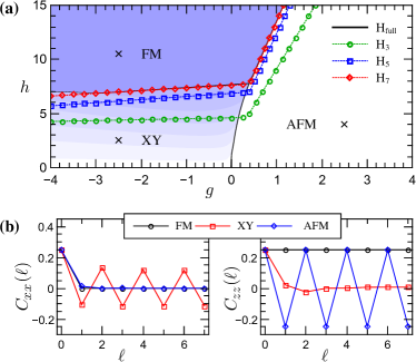
Figure 4: Edge Hamiltonian for the perturbed AKLT model, Eq. (1). (a) Phase diagram as a function of anisotropy $g$ and field $h$, for $J=1$. Three phases are observed: a fully polarized ferromagnetic (FM) phase (with magnetization $m_{z}=\tfrac{1}{2}$), an antiferromagnetic (AFM) phase ($m_{z}=0$), and an XY Luttinger liquid phase. The shading shows $m_{z}$ for the ground state of the full edge Hamiltonian $\mathcal{H}$ for $N_{v}=14$; the solid lines give phase boundaries determined analytically using fully polarized and mean-field AFM ansatzes, both for $\mathcal{H}$ and Hamiltonians $\mathcal{H}_{k}$ where the sum in (2) and (3) is restricted to $\ell<k$. (b) Correlation functions $C_{xx}(\ell)=\left\langle S_{i}^{x}S_{i+\ell}^{x}\right\rangle$ and $C_{zz}(\ell)=\left\langle S_{i}^{z}S_{i+\ell}^{z}\right\rangle$ for the three phases, computed at the points marked $\times$ in (a). DMRG calculations for $\mathcal{H}_{k}$ show that in the XY phase, $C_{xx}$ decays algebraically.

We have studied the phase diagram of the edge for $J>0$ using exact diagonalization supplemented by DMRG and analytical arguments, see Fig. 4. We find that the model exhibits three phases—a fully polarized ferromagnetic phase, an antiferromagnetic phase, and an XY Luttinger liquid phase. By choosing the appropriate bulk perturbation $V$, we can thus achieve either gapped, gapless, or symmetry broken phases at the edge, and induce phase transitions between them.

A natural question to ask at this point is whether we can achieve any edge Hamiltonian $\mathcal{H}$ we want. Since for a trivial bulk phase the mapping $\mathcal{X}$ from the edge to the bulk is injective, the answer there is indeed yes. Even more, any local $\mathcal{H}$ can be obtained from an approximately local bulk perturbation: At the RG fixed point where $A$ is the identity, this is clear. Now for any model connected to it via a gapped path, we can obtain its ground space via a quasi-adiabatic evolution Hastings and Wen (2005) of the original ground space; the correspondingly evolved bulk perturbation is then quasi-local and yields the desired $\mathcal{H}$. Thus, we find that for a trivial bulk phase, the edge is never protected .

We now turn towards topologically ordered systems, and investigate whether the bulk order can protect the physics at the edge. In these systems, the PEPS tensor is invariant under a symmetry action on the virtual indices which can be identified with particle types (charges) $p$ of the topological model. Therefore, the transfer operator $\mathbb{E}$ of a column, Fig. 2, is degenerate, with its maximal eigenvectors $\rho_{\mathrm{fp}}^{p}$ being supported on the sector with total topological charge $p$ Schuch et al. (2013). In particular, the fixed point $\mathbb{E}^{\infty}$ in Fig. 2b is of the form $\mathbb{E}^{\infty}=\sum_{p}|\rho_{\mathrm{fp},L}^{p}\rangle\langle\rho_{\mathrm{fp},R}^{p^{*}}|$, with $p^{*}$ the anti-particle of $p$.

Let us now for a moment fix $p$ in the sum: Then, we are essentially back in the scenario which we had for non-degenerate $\mathbb{E}$, in that any perturbation induces an effective edge Hamiltonian on the two edges independently. However, there is an important difference: $\rho_{\mathrm{fp},L}^{p}$ does not have full rank, but is supported on the sector with topological charge $p$. Thus, only boundary conditions $|\bm{\alpha})$ in this sector will correspond to a non-zero physical state $|\Phi_{\bm{\alpha}}\rangle$ and thus to admissible gapless excitations. At the same time, the label $p$ is also preserved by $\mathbb{E}_{V}$ (since it emerges from a symmetry acting solely on the virtual indices of the PEPS tensor Schuch et al. (2010)), and thus, $\mathcal{M}_{L}^{p}$ is also supported only in that sector. Thus, we can still orthogonalize it using the pseudoinverse of $(\rho_{\mathrm{fp},L}^{p})^{1/2}$, and obtain an effective edge Hamiltonian $\mathcal{H}_{L}^{p}$ for the sector with charge $p$; analogously, we obtain an edge Hamiltonian $\mathcal{H}_{R}^{p^{*}}$ for the right edge.

The full edge Hamiltonian is now obtained by putting both edges together and summing over $p$; it is of the form

$$\mathcal{H}=\Pi_{0}\,(\mathcal{H}_{L}\otimes\openone_{R}+\openone_{L}\otimes\mathcal{H}_{R})\,\Pi_{0}\ ,$$

where $\mathcal{H}_{L,R}=\sum_{p}\mathcal{H}_{L,R}^{p}$, and $\Pi_{0}$ is the projector onto the sector with total charge $p=0$ for both boundaries together. This implies that the edge Hamiltonian for a single edge must conserve the topological charge; this edge symmetry is protected by the topological order in the bulk and can stabilize non-trivial properties of the edge Hamiltonian Gu and Wen . Let us illustrate this for the Toric Code (TC) Kitaev (2003), where the spin-$\tfrac{1}{2}$ edge Hamiltonian is constrained by a quasi-fermionic $\mathbb{Z}_{2}$ parity superselection rule. Since the TC is an RG fixed point, there is a one-to-one local unitary correspondence between virtual and physical degrees of freedom at the edge up to the parity constraint Schuch et al. (2010), allowing to engineer any parity-preserving edge Hamiltonian. In particular, $V=-\sum_{\langle ij\rangle}S^{x}_{i}S^{x}_{j}$ yields Ising models $\mathcal{H}_{L}=\mathcal{H}_{R}=-\sum S^{x}_{i}S^{x}_{i+1}$ at the edges, whose even and odd parity ground states are the GHZ states $|+\ldots+\rangle\pm|-\ldots-\rangle$. Thus, each of the edges is an Ising model in a GHZ state—a macroscopic superposition—which is protected against spontaneous symmetry breaking by arbitrary local perturbations, something which is impossible in a conventional 1D spin system; this is in close analogy to the protection of a fermionic Majorana chain Kitaev (2001).

We have computed the edge Hamiltonian for the topological RVB state on the kagome lattice, which is a $D=3$ PEPS Verstraete et al. (2006); Schuch et al. (2012), for a bulk perturbation $V=\sum_{\langle i,j\rangle}\bm{S}_{i}\cdot\bm{S}_{j}$. We find that $\mathcal{H}_{L}$ and $\mathcal{H}_{R}$ are again approximately local, while the per-sector Hamiltonians $\mathcal{H}_{L/R}^{p}$ are not; the latter is due to the fact that $\mathcal{H}_{L/R}^{p}$ contain a projector onto a superselection sector, in direct analogy to what has been found for the Hamiltonians reproducing the entanglement spectrum in the case of topological models Schuch et al. (2013). The symmetry of the RVB PEPS strongly restricts the possible local terms, implying that the structure of the edge is that of a spinful particle or a hole, similar to a $t$-$J$ model Poilblanc et al. (2012); in that language and the notation of Poilblanc et al. (2012), the leading terms of the edge Hamiltonian for $N_{v}=8$ are a NN Heisenberg term ($J_{1}\approx 0.233$), chemical potential ($c_{2}\approx 0.177$), NN hopping ($t_{1}\approx-0.158$), and NN singlet creation ($\Delta_{1}\approx-0.086$). We have also considered a chiral perturbation $V=\sum\bm{S}_{i}\cdot(\bm{S}_{j}\times\bm{S}_{k})$, where the sum runs over all triangles, and found that the dominant term at the edge is given by a chiral current of particles, $\mathcal{H}_{L}\approx\sum ia_{s,k}^{\dagger}a^{\phantom{\dagger}}_{s,k+1}+\mathrm{h.c.}$, carrying $64.5\%$ of the total weight in $\mathcal{H}_{L}$. Note, however, that such a term by itself does not give rise to a protected chiral edge mode. [A similar chiral perturbation to the AKLT model gives in leading order rise to a chiral spin current $\mathcal{H}\approx\sum\bm{S}_{k}\cdot(\bm{S}_{k+1}\times\bm{S}_{k+2})$; this is the simplest $\mathrm{SU}(2)$ invariant spin-$\tfrac{1}{2}$ Hamiltonian.]

In this paper, we have studied edge theories in the framework of PEPS models. We have demonstrated that the effective low-energy theory lives on the virtual degrees of freedom at the boundary, which allows to explicitly obtain the edge Hamiltonian in the vicinity of these models. In the trivial phase, this allows to engineer arbitrary edge Hamiltonians, while topological bulk phases carry symmetries at their boundary which can protect the physics at the edge. Thus, protected physics at the edge is a signature of topological order in the bulk, and we expect that one can characterize the type of bulk topological order from the the protected properties of the edge inp . All results equally apply to fermionic systems Kraus et al. (2010). While we focused on a perturbative regime around PEPS models, we expect our findings to apply more generally: First, PEPS approximate ground states of local Hamiltonians well Hastings (2007) and any (generic) PEPS has a parent Hamiltonian associated with it Perez-Garcia et al. (2008); Schuch et al. (2010), suggesting that many systems have a PEPS model closeby; and second, the identification of the low-energy physics with the virtual degrees of freedom at the edge extends to any system connected to a PEPS model by a gapped path, by quasi-adiabatical evolution of the ground space Hastings and Wen (2005).

One question left open is the possible correspondence between entanglement spectrum and edge physics Li and Haldane (2008); Fidkowski (2009); Qi et al. (2012) beyond that emerging from their joint symmetry structure. E.g., for the RVB model the Heisenberg term in $\mathcal{H}$ is much enhanced as compared to the Hamiltonian derived from the entanglement spectrum Cirac et al. (2011); Poilblanc et al. (2012), this can be seen as a trace of the Heisenberg bulk perturbation. It would be interesting to study this further by applying our framework to frustrated PEPS models (such as variationally minimized iPEPS) which exhibit edge dynamics without perturbations.

We acknowledge helpful discussions with Z.-C. Gu, D. Pérez-García and J. Preskill. Parts of this work were done at the Simons Institute for the Theory of Computing in Berkeley, and at the Centro de Ciencias de Benasque Pedro Pascual in Benasque, Spain. N.S. and L.L. acknowledge support by the Alexander von Humboldt foundation and the EU project QALGO. D.P. acknowledges partial support by the Agence Nationale de la Recherche under grant No. ANR 2010 BLANC 0406-0. J.I.C. and F.V. acknowledge support by the EU project SIQS. F.V. acknowledges support from the FWF (Foqus and Vicom), the ERC (QUERG), and the FWO (Odysseus grant).

References

- Wen (1990) X.-G. Wen, Phys. Rev. B 41, 12838 (1990).
- Wen (1995) X.-G. Wen, Adv. Phys. 44, 405 (1995), arXiv:cond-mat/9506066 .
- (3) Z.-C. Gu and X.-G. Wen, arXiv:1201.2648 .
- Chen et al. (2012) X. Chen, Z.-C. Gu, Z.-X. Liu, and X.-G. Wen, Science 338, 1604 (2012), arXiv:1301.0861 .
- Kitaev (2003) A. Kitaev, Ann. Phys. 303, 2 (2003), quant-ph/9707021 .
- Affleck et al. (1988) A. Affleck, T. Kennedy, E. H. Lieb, and H. Tasaki, Commun. Math. Phys. 115, 477 (1988).
- Verstraete and Cirac (2004) F. Verstraete and J. I. Cirac, Phys. Rev. A 70, 060302 (2004), quant-ph/0311130 .
- Perez-Garcia et al. (2008) D. Perez-Garcia, F. Verstraete, J. I. Cirac, and M. M. Wolf, Quantum Inf. Comput. 8, 0650 (2008), arXiv:0707.2260 .
- Schuch et al. (2010) N. Schuch, I. Cirac, and D. Pérez-García, Ann. Phys. 325, 2153 (2010), arXiv:1001.3807 .
- Verstraete et al. (2006) F. Verstraete, M. M. Wolf, D. Perez-Garcia, and J. I. Cirac, Phys. Rev. Lett. 96, 220601 (2006), quant-ph/0601075 .
- Buerschaper et al. (2009) O. Buerschaper, M. Aguado, and G. Vidal, Phys. Rev. B 79, 085119 (2009), arXiv:0809.2393 .
- Gu et al. (2009) Z.-C. Gu, M. Levin, B. Swingle, and X.-G. Wen, Phys. Rev. B 79, 085118 (2009), arXiv:0809.2821 .
- Schuch et al. (2012) N. Schuch, D. Poilblanc, J. I. Cirac, and D. Pérez-García, Phys. Rev. B 86, 115108 (2012), arXiv:1203.4816 .
- Michalakis and Pytel (2011) S. Michalakis and J. Pytel, (2011), arXiv:1109.1588 .
- Cirac et al. (2013) J. Cirac, S. Michalakis, D. Perez-Garcia, and N. Schuch, Phys. Rev. B 88, 115108 (2013), arXiv:1306.4003 .
- Perez-Garcia et al. (2007) D. Perez-Garcia, F. Verstraete, M. M. Wolf, and J. I. Cirac, Quant. Inf. Comput. 7, 401 (2007), quant-ph/0608197 .
- Perez-Garcia et al. (2010) D. Perez-Garcia, M. Sanz, C. E. Gonzalez-Guillen, M. M. Wolf, and J. I. Cirac, New J. Phys. 12, 025010 (2010), arXiv.org:0908.1674 .
- Cirac et al. (2011) J. I. Cirac, D. Poilblanc, N. Schuch, and F. Verstraete, Phys. Rev. B 83, 245134 (2011), arXiv:1103.3427 .
- Schuch et al. (2013) N. Schuch, D. Poilblanc, J. I. Cirac, and D. Perez-Garcia, Phys. Rev. Lett. 111, 090501 (2013), arXiv:1210.5601 .
- Note (1) Applying on the physical index of translates to applying the sum of to the virtual indices. When applying , the sum of the appearing at the two ends of each singlet cancel, and one is left with the at the boundary. Thus, , and the claim follows. The same argument holds for the response of arbitrary models with on-site symmetries to local fields.
- Hastings and Wen (2005) M. B. Hastings and X. Wen, Phys. Rev. B 72, 045141 (2005), cond-mat/0503554 .
- Note (2) Note that it is still possible to protect edge properties by symmetries in the bulk Gu and Wen ; Chen et al. (2012)—e.g., in the AKLT model, symmetry rules out a gapped edge which does not break any symmetry Lieb et al. (1961).
- Kitaev (2001) A. Kitaev, Phys.-Usp. 44, 131 (2001), cond-mat/0010440 .
- Poilblanc et al. (2012) D. Poilblanc, N. Schuch, D. Pérez-García, and J. I. Cirac, Phys. Rev. B 86, 014404 (2012), arXiv:1202.0947 .
- (25) J.I. Cirac, N. Schuch, and F. Verstraete, in preparation.
- Kraus et al. (2010) C. V. Kraus, N. Schuch, F. Verstraete, and J. I. Cirac, Phys. Rev. A 81, 052338 (2010), arXiv:0904.4667 .
- Hastings (2007) M. B. Hastings, Phys. Rev. B 76, 035114 (2007), cond-mat/0701055 .
- Li and Haldane (2008) H. Li and F. D. M. Haldane, Phys. Rev. Lett. 101, 010504 (2008), arXiv:0805.0332 .
- Fidkowski (2009) L. Fidkowski, (2009), arXiv:0909.2654 .
- Qi et al. (2012) X.-L. Qi, H. Katsura, and A. W. W. Ludwig, Phys. Rev. Lett. 108 (2012), arXiv:1103.5437 .
- Lieb et al. (1961) E. H. Lieb, T. D. Schultz, and D. C. Mattis, Ann. Phys. (N. Y.) 16, 407 (1961).