Observational constraints on G-corrected holographic dark energy using a Markov chain Monte Carlo method

Abstract

We constrain holographic dark energy (HDE) with time varying gravitational coupling constant in the framework of the modified Friedmann equations using cosmological data from type Ia supernovae, baryon acoustic oscillations, cosmic microwave background radiation and X-ray gas mass fraction. Applying a Markov Chain Monte Carlo (MCMC) simulation, we obtain the best fit values of the model and cosmological parameters within $1\sigma$ confidence level (CL) in a flat universe as: $\Omega_{\rm b}h^{2}=0.0222^{+0.0018}_{-0.0013}$, $\Omega_{\rm c}h^{2}=0.1121^{+0.0110}_{-0.0079}$, $\alpha_{\rm G}\equiv\dot{G}/(HG)=0.1647^{+0.3547}_{-0.2971}$ and the HDE constant $c=0.9322^{+0.4569}_{-0.5447}$. Using the best fit values, the equation of state of the dark component at the present time $w_{\rm d0}$ at $1\sigma$ CL can cross the phantom boundary $w=-1$.

keywords: Cosmology, dark energy, holographic model, gravitational constant.

I Introduction

The astronomical data from ”Type Ia supernova” Riess:1998cb ; Perlmutter:1998np indicate that the current universe is in an accelerating phase. These observational results have greatly inspirited theorists to understand the mechanism of this accelerating expansion. In the framework of standard cosmology, an exotic energy with negative pressure, the so-called dark energy, is attributed to this cosmic acceleration.

Up to now, some theoretical models have been presented to explain the dynamics of dark energy and cosmic acceleration of the universe. The simplest but most natural candidate is the cosmological constant $\Lambda$, with a constant equation of state (EoS) $w=-1$ Sahni:1999gb ; Peebles:2002gy . As we know, the cosmological constant confronts us with two difficulties: the fine-tuning and cosmic coincidence problems. In order to solve or alleviate these problems many dynamical dark energy models with time-varying EoS have been proposed. The quintessence Wetterich:1987fm ; Ratra:1987rm , phantom Caldwell:1999ew ; Nojiri:2003vn ; Nojiri:2003jn , quintom Elizalde:2004mq ; Nojiri:2005sx ; Anisimov:2005ne , K-essence ArmendarizPicon:2000dh ; ArmendarizPicon:2000ah , tachyon Padmanabhan:2002cp ; Sen:2002in , ghost condensate ArkaniHamed:2003uy ; Piazza:2004df , agegraphic Cai:2007us ; Wei:2007ty and holographic Witten:2000zk are examples of dynamical models. Although many dynamical dark energy models have been suggested, the nature of dark energy is still unknown.

Models which are constructed based on fundamental principles are more preferred as they may exhibit some underlying features of dark energy. Two examples of such kind of dark energy models are the agegraphic Cai:2007us ; Wei:2007ty and holographic Hsu:2004ri ; Li:2004rb models. In this work we focus on the holographic dark energy model. The holographic model is built on the basis of the holographic principle and some features of quantum gravity theory Witten:2000zk . According to the holographic principle, the number of degrees of freedom in a bound system should be finite and is related to the area of its boundary. In holographic principle, a short distance ultra-violet (UV) cut-off is related to the long distance infra-red (IR) cut-off, due to the limit set by the formation of a black hole Horava:2000tb ; Thomas:2002pq . The total energy of a system with size $L$ should not exceed the mass of a black hole with the same size, i.e., $L^{3}\rho_{\rm d}\leq LM_{pl}^{2}$. Saturating this inequality, the holographic dark energy density is obtained as

$$\rho_{\rm d}=\frac{3c^{2}}{8\pi GL^{2}}\;,$$ (1)

where L is the length of the horizon, $c$ is a numerical constant of model and $G$ is the gravitational coupling constant.
The UV cut-off is related to the vacuum energy and the IR cut-off is related to the large scale of the universe, such as Hubble horizon, particle horizon, event horizon, Ricci scalar or the generalized functions of dimensionless variables as discussed by Hsu:2004ri ; Li:2004rb ; Gao:2007ep ; Xu:2009xi . If we consider the Hubble length scale for $L$, it leads to wrong equation of state for dark energy, i.e., $w_{d}=0$ which can not result the cosmic acceleration Horava:2000tb ; Thomas:2002pq . This problem can be cured by considering the interaction between dark matter and dark energy Pavon:2005yx ; Zimdahl:2007zz . In the case of particle horizon, the EoS of dark energy is bigger than $-1/3$, hence the current accelerated expansion can not be well explained Pavon:2005yx ; Zimdahl:2007zz . Holographic dark energy with event horizon can provide a desired EoS to describe the cosmic acceleration Zhou:2007pz ; Sheykhi:2009zv . Nojiri and Odintsov investigated the HDE model by assuming IR cutoff depends on the Hubble rate, particle and future horizons Nojiri:2005pu . In this generalized form the phantom regime can be achieved and also the coincidence problem is demonstrated. Unification of early phantom inflation and late time acceleration of the universe is another feature of this model.

In recent years, the HDE model has been constrained by various cosmological observations Huang:2004wt ; Enqvist:2004ny ; Enqvist:2004ny ; Shen:2004ck ; Zhang:2005hs ; Kao:2005xp ; Wu:2007fs ; Ma:2007pd ; Zhang:2007sh ; Lu:2009iv ; Zhai:2011pp ; Zhang:2013mca . For example, Huang and Gong in Huang:2004wt obtained the parameter $c$ as $c=0.21$ by using the SNIa observations. Enqvist et.al. in Enqvist:2004ny found a connection between the holographic dark energy and low-$l$ CMB multipoles by using CMB, LSS and supernovae data. Zhang et.al. by using the OHD data constrained the parameter $c$ as $c=0.65^{+0.02}_{-0.03}$ Zhai:2011pp .

Beside, there are some theoretical and observational evidences indicating that the gravitational coupling constant $G$ varies with cosmic time $t$. From the theoretical viewpoint one can be referred to the works of DiracDirac:1938mt and Dyson Dyson:1972 ; Lannutti:1978dv . In Branse-Dicke theory, the variability of $G$ is also predicted Brans:1961sx . In Kaluza-Klein cosmology, time varying treatment of $G$ is related to the scalar field appearing in the metric component corresponding to the 5-th dimension Kaluza:1921tu ; LorenAguilar:2003kx ; Kolb:1985sj ; Maeda:1985bq ; Freund:1982pg . In this case, a scalar field couples with gravity by definition of a new parameter. From observational point of view, the value of the parameter $\dot{G}/G$ (where an overdot represents derivative with respect to the cosmic time $t$) can be constrained by astrophysical and cosmological observations as well. For example data from SNIa observations yields $-10^{-11}{\rm yr^{-1}}\leq{\dot{G}}/{G}\leq 0$ Gaztanaga:2001fh . The observations of the Binary Pulsar PSR1913 gives $-(1.10\pm 1.07)\times 10^{-11}{\rm yr^{-1}}\leq{\dot{G}}/{G}\leq 0$ Damour:1988zz . The observational data from the Big Bang nuclei-synthesis results tighter constraints on this parameter as $-3.0\times 10^{-13}{\rm yr^{-1}}\leq{\dot{G}}/{G}\leq 4.0\times 10^{-13}{\rm yr^{-1}}$ Copi:2003xd . This parameter can be approximated from astro-seismological data from pulsating white dwarf stars Benvenuto:2004bs ; Biesiada:2003sr and helio-sesmiological 0004-637X-498-2-871 as well.

All mentioned above motivated people to consider the holographic dark energy model with time varying gravitational coupling $G$ (G-corrected HDE model) enveloped by event horizon. In Jamil:2009sq ; Lu:2009iv , the holographic model with varying gravitational coupling $G$ was assumed in the standard Friedmann equations. The authors in Malekjani:2013xsa considered the G-corrected HDE in the framework of the modified Friedmann equations. The holographic model with varying $G$ in the standard Friedmann equations has been constrained by cosmological data in Lu:2009iv where for a flat universe they found $c=0.80^{+0.16}_{-0.13}$ and $\alpha_{\rm G}\equiv\dot{G}/(HG)=-0.0016^{+0.0049}_{-0.0019}$. In this paper, by using the cosmological data of Type Ia Supernovae (SNIa), Baryon Acoustic Oscillations (BAO), Cosmic Microwave Background (CMB) radiation and X-ray gas mass fraction we will obtain the best fit values of parameters of the G-corrected HDE in the framework of the modified Friedmann equations by applying a Markov Chain Monte Carlo (MCMC) simulation. Based on these best fit values, we obtain the evolution of EoS and deceleration parameter $q$ of the $G$-corrected HDE model as well as the evolution of energy density parameters. We show that within $1\sigma$ confidence level, this model can cross the phantom boundary $w=-1$.

The paper is organized as follows: In section II the $G$-corrected HDE is discussed briefly. Then in section III the cosmological constraining method is discussed in detail and the data fitting results are presented in section IV. The paper is concluded in section V.

II G-corrected HDE model in a FRW cosmology

The Hilbert-Einstein action with time varying gravitational coupling constant, $G(t)=G_{0}\phi(t)$, is described as

$$S=\frac{1}{16\pi G_{0}}\int{\sqrt{-g}\left(\frac{R}{\phi(t)}+L_{m}\right)d^{4}x}$$ (2)

where the scalar function $\phi(t)$ is assumed for time dependency of $G(t)=\phi(t)G_{0}$, $G_{0}$ is the bare gravitational coupling constant and $L_{m}$ is the lagrangian of the matter fields. The first modified Friedmann equation for Robertson-Walker spacetime is obtained as Malekjani:2013xsa

$$H^{2}=\frac{8\pi G(t)}{3}(\rho_{\rm m}+\rho_{\rm d})+H\frac{\dot{G}}{G}$$ (3)

where an overdot represents the derivative with respect to the cosmic time t, $H=\dot{a}/a$ and $\rho_{\rm m}$ and $\rho_{\rm d}$ are matter and dark energy densities respectively. We ignore the higher time derivative of $G$ (i.e., $\ddot{G}/G$, …) and also higher powers than one (i.e., ($\dot{G}/G)^{2}$, …), since the value of $\dot{G}/G$ is small particularly in the late time accelerated universe. The last term on right hand side of (3) is due to the correction of time dependency of $G$. Equation (3) can also be obtained from Branse-Dicke gravity by assuming $w=0$ and $\psi=1/\phi(t)$ in equation (1) of Banerjee:2007zd where $w$ is the Branse-Dicke parameter and $\psi$ is Branse-Dicke scalar field.
Changing the time derivative to a derivative with respect to $\ln{a}$, equation (3) is expressed as:

$$H^{2}(1-\alpha_{\rm G})=\frac{8\pi G(t)}{3}(\rho_{\rm m}+\rho_{\rm d}),$$ (4)

where $\alpha_{\rm G}={\acute{G}}/{G}$ and the prime represents derivative with respect to $\ln a$. Putting $\alpha_{\rm G}=0$ and $G(t)=G_{0}$, equation 4 reduces to the standard Friedmann equation in flat universe.
The energy density of the $G$-corrected HDE model, by assuming the event horizon IR cut-off $R_{\rm h}=a\int{\tfrac{dt}{a}}=a\int{\tfrac{H}{\acute{a}}d\acute{a}}$, is given by

$$\rho_{\rm d}=\frac{3c^{2}}{8\pi G(t)R_{\rm h}^{2}}\;.$$ (5)

Using the definition of dimensionless energy density parameters $\Omega_{\rm m}=\rho_{\rm m}/\rho_{\rm cr}$ and $\Omega_{\rm d}=\rho_{\rm d}/\rho_{\rm cr}$, where $\rho_{\rm cr}=3H^{2}/8\pi G(t)$, the modified Friedmann equation (4) can be rewritten as

$$\Omega_{\rm m}+\Omega_{\rm d}=1-\alpha_{\rm G}\;.$$ (6)

The matter (baryonic and CDM) and dark energy satisfy the following conservation equation

$$\dot{\rho}_{m}+3H\rho_{\rm m}=0\;,$$ (7a)

$$\dot{\rho}_{\rm d}+3H(1+w_{\rm d})\rho_{\rm d}=0,$$ (7b)

respectively, where $w_{\rm d}$ is the dark energy EoS. The Hubble parameter in the context of $G$-corrected HDE model in a flat geometry can be calculated from Eq. (3) as follows

$$H^{2}(1-\alpha_{\rm G})={H_{0}}^{2}[\Omega_{\rm m0}a^{-3}+\Omega_{\rm d0}a^{-3(1+w_{\rm d})}],$$ (8)

where $H_{0}$ is the present value of Hubble parameter and $\Omega_{\rm m0}$ and $\Omega_{\rm d0}$ are the present values of the density parameters of matter (baryonic and CDM) and dark energy respectively. Taking the time derivative of (5) by using conservation equation (7b) as well as the relation $\dot{R}_{h}=1+HR_{\rm h}$ the equation of state for the G-corrected HDE model can be obtained as

$$w_{\rm d}=-\frac{1}{3}-\frac{2}{3}\frac{\sqrt{\Omega_{\rm d}}}{c}+\frac{1}{3}\alpha_{\rm G}\;.$$ (9)

The evolutionary equation of the dark energy density parameter $\Omega_{\rm d}$ for the G-corrected HDE model can be obtained by taking derivative of $\Omega_{\rm d}=\tfrac{\rho_{\rm d}}{\rho_{\rm cr}}=\tfrac{c^{2}}{H^{2}R_{\rm h}^{2}}$ with respect to $\ln{a}$ as follows

$$\acute{\Omega_{\rm d}}=-2\Omega_{\rm d}[\frac{c}{HR}+\frac{\dot{H}}{H^{2}}+1]\;.$$ (10)

Also, taking the time derivative of the modified Friedmann equation (3) yields

$$\frac{\dot{H}}{H^{2}}(1-\frac{1}{2}\alpha_{\rm G})=-\frac{3}{2}(1+w_{d}\Omega_{\rm d})+2\alpha_{\rm G}\;.$$ (11)

Inserting (11) in (10) results

$$\acute{\Omega_{\rm d}} (1-\alpha_{\rm G}/2)=\Omega_{\rm d}\Big{(}3(1+w_{d}\Omega_{\rm d})+\frac{\sqrt{\Omega_{\rm d}}}{c}(2-\alpha_{\rm G})-3\alpha_{\rm G}-2\Big{)}\;.$$ (12)

The deceleration parameter $q=-1-\dot{H}/H^{2}$ for determining the accelerated phase of the expansion ($q<0$) or decelerated phase ($q>0$) can be obtained for the $G$-corrected HDE model by using (11) as

$$q(1-\frac{1}{2}\alpha_{\rm G})=\frac{1}{2}(1+3w_{d}\Omega_{\rm d})-\frac{3}{2}\alpha_{\rm G}\;.$$ (13)

At early times when the energy density of dark energy tends to zero and also the correction of $G$ is negligible, one can see that $q\rightarrow 1/2$, representing deceleration phase in the CDM model. In the limiting case of time-independent gravitational constant G (i.e., $\alpha_{\rm G}=0$) all the above relations reduce to those obtained for original holographic dark energy (OHDE) model in Zhang:2005yz .

III Data Fitting method

The constant $c$ and the quantity $\dot{G}/G$ determine evolution of the universe in the G-corrected holographic dark energy model. Therefor to study the cosmic evolution in the G-corrected HDE in the framework of the modified Friedmann equations, it is of great importance to constrain these parameters by cosmological data.

In this section we discuss the method for obtaining the best fit values of the G-corrected HDE parameters by using the cosmological data. The fitting method which we use is the maximum likelihood method. In this method the total likelihood function $\mathcal{L}_{\rm tot}=e^{-\chi^{2}_{\rm tot}/2}$ is maximized by minimizing $\chi^{2}_{\rm tot}$. To determine $\chi^{2}_{\rm tot}$ we use the following observational data set: cosmic microwave background radiation (CMB) data from the seven-year WMAP Komatsu:2010fb , type Ia supernova (SNIa) data from 557 Union2 Union2 , baryon acoustic oscillation (BAO) data from SDSS DR7 Percival:2009xn , and cluster X-ray gas mass fraction data which is measured by Chandra X-ray telescope observations Allen:2007ue . Therefor $\chi^{2}_{\rm tot}$ is given by the relation

$$\chi^{2}_{\rm tot}=\chi^{2}_{\rm SNIa}+\chi^{2}_{\rm CMB}+\chi^{2}_{\rm BAO}+\chi^{2}_{\rm gas}\;.$$ (14)

In following we discuss each $\chi^{2}$ in detail.

The data for SNIa are 557 Union2 data Union2 . In this case $\chi^{2}_{\rm SNIa}$ is obtained by comparing the theoretical distance modulus $\mu_{\rm th}(z)$ with the observed one $\mu_{\rm ob}(z)$

$$\chi^{2}_{\rm SNIa}=\sum_{\rm i}\frac{[\mu_{\rm th}(z_{i})-\mu_{\rm obs}(z_{i})]^{2}}{\sigma_{\rm i}^{2}}\;,$$ (15)

with

$$\mu_{\rm th}(z)=5\log_{10}[D_{\rm L}(z)]+\mu_{0}\;,$$ (16)

where $\mu_{0}=5\log_{10}(cH_{0}^{-1}/Mpc)+25$ and the observational modulus distance of SNIa, $\mu_{\rm obs}(z_{i})$, at redshift $z_{i}$ is given by

$$\mu_{\rm obs}(z_{i})=m_{\rm obs}(z_{i})-M,$$ (17)

where $m$ and $M$ are apparent and absolute magnitudes of SNIa respectively. The Hubble-free luminosity distance $D_{\rm L}$ is given by

$$d_{\rm L}(z)=\frac{H_{0}(1+z)}{\sqrt{|\Omega_{\rm k}|}}sinn[\sqrt{|\Omega_{\rm k}|}\int_{0}^{z}\frac{dz^{\prime}}{H(z^{\prime})}]\;,$$ (18)

where $sinn(\sqrt{|\Omega_{\rm k}|}x)$ represents respectively $sin(\sqrt{|\Omega_{\rm k}|}x)$, $\sqrt{|\Omega_{\rm k}|}$ and $sinh(\sqrt{|\Omega_{\rm k}|})$ for $\Omega_{\rm k}<0$, $\Omega_{\rm k}=0$ and $\Omega_{\rm k}>0$. Eq. (15) can be written Nesseris:2007pa

$$\chi^{2}_{SNIa}=A+2B\mu_{0}+C\mu_{0}^{2}\;,$$ (19)

where

$$A =\sum_{i}\frac{[\mu_{\rm th}(z_{i};\mu_{0}=0)-\mu_{\rm obs}(z_{i})]^{2}}{\sigma_{\rm i}^{2}}$$ (20a)

$$B =\sum_{i}\frac{\mu_{\rm th}(z_{i};\mu_{0}=0)-\mu_{\rm obs}(z_{i})}{\sigma_{\rm i}^{2}}$$ (20b)

$$C =\sum_{i}\frac{1}{\sigma_{\rm i}^{2}}$$ (20c)

where $\mu_{0}=42.384-5\log_{10}h$. The minimum of eq. (15) can be written as

$$\chi^{2}_{\rm SNIa,min}=A-B^{2}/C\;.$$ (21)

The goodness of fit between the theoretical model and data is expressed by $\chi^{2}_{\rm SNIa,min}$.

For the CMB data, we use the data points $(R,l_{\rm a},z_{\ast})$ from seven-year WMAP Komatsu:2010fb . The data points parameters are as follows: $R$ is the scaled distance to recombination $R=\sqrt{\Omega_{\rm m0}/c}\int_{0}^{z_{\ast}}dz/E(z)$, where $E(z)\equiv H(z)/H_{0}$ and $z_{\ast}$ is recombination redshift Hu:1995en . The angular scale of the sound horizon at recombination is given by $l_{\rm A}$ Bond:1997wr

$$l_{\rm A}=\frac{\pi r(z_{\ast})}{r_{\rm s}(z_{\ast})}\;\;,$$ (22)

where $r(z)$ is the comoving distance $r(z)=c/H_{0}\int_{0}^{z}dz^{\prime}/E(z^{\prime})$ and the comoving sound horizon distance at the recombination $r_{\rm s}(z_{\ast})$ is given by

$$r_{\rm s}(z_{\ast})=\int_{0}^{a(z_{\ast})}\frac{c_{\rm s}(a)}{a^{2}H(a)}da\;,$$ (23)

where the sound speed $c_{\rm s}(a)$ is defined by

$$c_{\rm s}(a)=\left[3(1+\frac{3\Omega_{\rm b0}}{4\Omega{\gamma 0}}a)\right]^{-1/2}\;,$$ (24)

Seven-year WMAP observations give $\Omega_{\rm\gamma 0}=2.469\times 10^{-5}h^{-2}$ and $\Omega_{\rm b0}=0.02260\pm 0.00053\times 10^{-5}h^{-2}$ Komatsu:2010fb .

The recombination redshift $z_{\ast}$ is obtained using the fitting function proposed by Hu and Sugiyama Hu:1995en

$$z_{\ast}=1048[1+0.00124(\Omega_{\rm b0}h^{2})^{-0.738}][1+g_{\rm 1}(\Omega_{\rm m0}h^{2})^{g_{2}}]\;,$$ (25)

where $g_{1}=(0.0783(\Omega_{\rm b0}h^{2})^{-0.238})/(1+39.5(\Omega_{\rm b0}h^{2})^{0.763})$ and $g_{2}=({0.560})/(1+21.1(\Omega_{\rm b0}h^{2})^{1.81})$. Then one can define $\chi^{2}_{\rm CMB}$ as $\chi^{2}_{\rm CMB}=X^{T}C^{-1}_{\rm CMB}X$, with Komatsu:2010fb

$$X =\begin{pmatrix}l_{\rm A}-302.09\\ R-1.725\\ z_{\ast}-1091.3\end{pmatrix},$$ (26a)

$$C^{-1}_{\rm CMB} =\begin{pmatrix}2.305&29.698&-1.333\\ 293689&6825.270&-113.180\\ -1.333&-113.180&3.414\end{pmatrix},$$ (26b)

where $C^{-1}_{\rm CMB}$ is the inverse covariant matrix.

The data from Sloan Digital Sky Survey (SDSS) Data Release 7 (DR7) Percival:2009xn is used for the baryon acoustic oscillations (BAO) data. One can define $\chi^{2}_{\rm BAO}$ by $\chi^{2}_{\rm BAO}=Y^{T}C^{-1}_{\rm BAO}Y$, where

$$Y =\begin{pmatrix}d_{0.2}-0.1905\\ d_{0.35}-0.1097\end{pmatrix}\;,$$ (27a)

$$C^{-1}_{\rm BAO} =\begin{pmatrix}30124&-17227\\ -17227&86977\end{pmatrix}\;.$$ (27b)

The data points $d_{z_{i}}$ is defined as $d_{\rm z_{i}}\equiv r_{\rm s}(z_{\rm d})/D_{\rm V}(z_{i})$, where $r_{\rm s}(z_{\rm d})$ is the comoving sound horizon distance at the drag epoch (where baryons were released from photons) and $D_{\rm V}$ is given by Eisenstein:2005su

$$D_{\rm V}(z)\equiv\left[\left(\int_{0}^{z}\frac{dz^{\prime}}{H(z^{\prime})}\right)^{2}\frac{cz}{H(z)}\right]^{1/3}\;.$$ (28)

The drag redshift is given by the fitting formula Eisenstein:1997ik

$$z_{\rm d}=\frac{1291(\Omega_{\rm m0}h^{2})^{0.251}}{1+0.659(\Omega_{\rm m0}h^{2})^{0.828}}\left[1+b_{1}(\Omega_{\rm b0}h^{2})^{b_{2}}\right]\;,$$ (29)

where $b_{1}=0.313(\Omega_{\rm m0}h^{2})^{-0.419}[1+0.607(\Omega_{\rm m0}h^{2})^{0.607}]$ and $b_{2}=0.238(\Omega_{\rm m0}h^{2})^{0.223}$.

The final data we use is X-ray gas mass fraction data from the Chandra X-ray observations Allen:2007ue . In this case we use the definition $\chi^{2}_{\rm gas}$

$$\chi^{2}_{\rm gas} = \sum_{i}^{N}\frac{[f_{\rm gas}^{\Lambda CDM}(z_{i})-f_{\rm gas}(z_{i})]^{2}}{\sigma_{\rm f_{\rm gas}}^{2}(z_{i})}+\frac{(s_{0}-0.16)^{2}}{0.0016^{2}}$$

$$+ \frac{(K-1.0)^{2}}{0.01^{2}}+\frac{(\eta-0.214)^{2}}{0.022^{2}}\;,$$

where $s_{0}=(0.16\pm 0.05)h_{70}^{0.5}$, $K=1.0\pm 0.1$ and $\eta=0.214\pm 0.022$ Allen:2007ue . The details for the from of the mass gas fractions $f_{\rm gas}(z)$ and $f_{\rm gas}^{\rm\Lambda CDM}$ is discussed in Allen:2007ue .

IV Data fitting results

Finally we apply a Markov Chain Monte Carlo simulation on the G-corrected HDE model by modifying the publically available CosmoMC code cosmomc . The parameter space is chosen as $(\Omega_{\rm b}h^{2},\Omega_{\rm c}h^{2},\alpha_{\rm G},c)$ with the priors $\Omega_{\rm b}h^{2}=[0.005,\;0.1]$, $\Omega_{\rm c}h^{2}=[0.01,\;0.99]$, $\alpha_{\rm G}=[-1,\;+1]$ and $c=[0,\;2]$. We also consider the derived parameters $(\Omega_{d},\;H_{0},\;{\rm age})$ as well. The results of the best fit values are presented in table 1. In addition figure 1 shows the 2-dimensional constraints of the cosmological parameters contours with $1\sigma$ and $2\sigma$ confidence levels.

Parameter	Best Fit Value	$\Lambda$CDM
$\Omega_{\rm b}h^{2}$	$0.0222^{+0.0018+0.0021}_{-0.0013-0.0016}$	$0.02214\pm 0.00024$
$\Omega_{\rm c}h^{2}$	$0.1121^{+0.0110+0.0130}_{-0.0079-0.0096}$	$0.1187\pm 0.0017$
$\Omega_{\rm d}$	$0.7246^{+0.0342+0.0418}_{-0.0485-0.0606}$	$0.692\pm 0.010$
$c$	$0.9322^{+0.4569}_{-0.5447}$	$\ldots$
$\alpha_{\rm G}$	$0.1647^{+0.3547+0.3576}_{-0.2971-0.2978}$	$\ldots$
$H_{0}$	$69.8809^{+3.5339+4.1638}_{-3.4423-4.4567}$	$67.80\pm 0.77$
Age (Gyr)	$13.8094^{+0.2801+0.3776}_{-0.3618-0.4392}$	$13.798\pm 0.45$

Table 1: The best fit values of the cosmological and model parameters in the G-corrected HDE model with $1\sigma$ and $2\sigma$ regions. Here the CMB, SNIa, BAO and X-ray gas mass fraction data together with the BBN constraints have been used. For comparison, the results for the $\Lambda$CDM model from the Planck data are presented in the third column Ade:2013zuv .

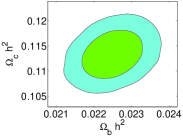
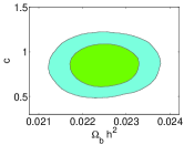
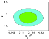
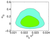
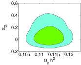
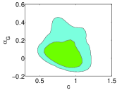
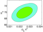
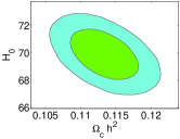
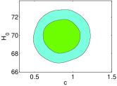
Figure 1: 2-dimensional constraint of the cosmological and model parameters contours in the G-corrected HDE model with $1\sigma$ and $2\sigma$ regions. To produce these plots, SNIa+CMB+BAO+X-ray gas mass fraction data sets together with the BBN constraints have been used.

From table 1 one can see that all main cosmological parameters ($\Omega_{\rm b}h^{2}$, $\Omega_{\rm c}h^{2}$, $\Omega_{\rm d}$, $H_{0}$, age) are in agreement with the results of the $\Lambda$CDM model Ade:2013zuv as one can see in the third column. The best fit value of the parameter $c$ i.e. $c=0.9322^{+0.4569}_{-0.5447}$ is also compatible with other works such as $c=0.91^{+0.21}_{-0.18}$ in Zhang:2007sh , $c=0.84^{+0.14}_{-0.12}$ in Zhang:2013mca and $c=0.68^{+0.03}_{-0.02}$ in Zhai:2011pp . Then by using the best fit values of parameters $\alpha_{\rm G}$ and $H_{0}$ one can obtain approximately the best fit value of quantity $\dot{G}/G=+1.14\times 10^{-11}{\rm yr^{-1}}$. This results is in agreement with the results of other constraining works. For example the astroseismological data obtained from pulsating white dwarf stars result $-2.5\times 10^{-10}{\rm yr^{-1}}\leq{\dot{G}}/{G}\leq+4.5\times 10^{-10}{\rm yr^{-1}}$ Benvenuto:2004bs and observations of the pulsating white dwarf G117-B15A suggest ${\dot{G}}/{G}\leq+4.1\times 10^{-11}{\rm yr^{-1}}$ Biesiada:2003sr . Therefore these two best values offer a self-consistency for our analysis. Lu et.al. in Lu:2009iv constrained HDE with varying gravitational coupling constant by using SNIa, CMB, BAO and OHD (Observational Hubble Data) data in the standard Friedmann equations framework. They found the best fit values: $c=0.80^{+0.16}_{-0.13}$ and $\alpha_{\rm G}=-0.0016^{+0.0049}_{-0.0019}$. Our results in $1\sigma$ CL are comparable with the Lu et. al. results as well.

Then we calculate the evolution of some cosmological quantities: EoS parameter of the dark energy component $w_{\rm d}$, matter and dark energy density parameters, and deceleration parameter for the G-corrected HDE model based on the best fit values of cosmological parameters in table 1. In the top-row of figure 2, the evolution of the EoS parameter $w_{d}$ (left panel) and the deceleration parameter $q$ (right panel) in terms of the redshift parameter $z$ has been plotted by solving equations (12) and (13) and using (9). We see that by using the best fit values in the G-corrected HDE model, within $1\sigma$ confidence level, one obtains the present value of EoS parameter as: $−1.887<w_{\rm d0}<-0.232$ which can enters to the phantom regime in lower bound. It is worthwhile to mention that in this case the phantom regime can be achieved without invoking interaction between dark matter and dark energy. In the left panel, the parameter $q$ can transit from positive values $q>0$ to negative values ($q<0$) which indicates the transition from early decelerated expansion to current accelerated phase of expansion. The present value of the deceleration parameter $q$ within $1\sigma$ confidence level is obtained as: $−1.1268<q_{0}<−0.5565$. Finally, the evolution of density parameters of dark energy and pressure-less matter has been shown in the bottom row figure 2. The density parameter of the pressureless matter decreases and dark energy increases by decreasing redshift, indicating the early time CDM dominated universe and current dark energy dominated phase in G-corrected HDE cosmology.

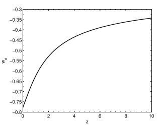
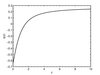
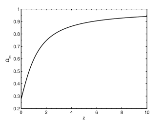
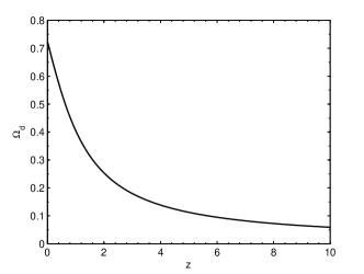
Figure 2: The evolution of EoS parameter $w_{d}$ (left-top panel), deceleration parameter $q$ (right-top panel), mater density parameter $\Omega_{\rm m}$ (left-bottom panel) and dark energy density parameter $\Omega_{\rm d}$ (right-bottom panel) for the best fit values in the $G$-corrected HDE model.

V conclusion

We performed cosmological constrains on the parameters of the holographic dark energy model with time varying gravitational coupling $G$ using a Markov chain Monte Carlo simulation. We used the SNIa, CMB, BAO and X-ray mass gas fraction data for data fitting. In the framework of the modified Friedmann equations, we obtained the best fit values for the cosmological parameters as: the physical baryon matter density $\Omega_{\rm b}h^{2}=0.0222^{+0.0018+0.0021}_{-0.0013-0.0016}$, dark matter physical density $\Omega_{\rm c}h^{2}=0.1121^{+0.0110+0.0130}_{-0.0079-0.0096}$, Hubble parameter at the current time $H_{0}=69.8809^{+3.5339+4.1638}_{-3.4423-4.4567}$ and the age of the Universe $13.8094^{+0.2801+0.3776}_{-0.3618-0.4392}$. We constrained the G-corrected HDE parameters $c$ and $\alpha_{\rm G}$ as well. The best fit value of the parameter $c=0.9322^{+0.4569}_{-0.5447}$ is in agreement with results of the previous works Zhang:2013mca ; Zhai:2011pp ; Lu:2009iv . In our model the best fit value for the rate of changing the gravitational coupling constant with time is $\dot{G}/G=+1.14\times 10^{-11}{\rm yr^{-1}}$. This value is close to the value obtained by others like constraints in Benvenuto:2004bs ; Biesiada:2003sr . Therefore the result of our analysis is compatible with observations and other analysis of the HDE model and time varying gravitational coupling constant.

The evolution of the deceleration parameter $q$, for the best fit values of cosmological parameters, indicates the transition from past decelerated to current accelerated expansion. By using the best fit values of the aforementioned parameters, within $1\sigma$ CL, the phantom regime $w<-1$ can be achieved in this model.

In summary we conclude that the holographic dark energy with a time varying gravitational coupling constant in the framework of the modified Friedmann equations, could be a candidate to describe the accelerated expansion of the universe. In addition, in future works, by using the data from Planck Ade:2013zuv and nine-year WMAP Bennett:2012zja projects, one can make the constraints on the model parameters even tighter.

References

References

- (1) Supernova Search Team Collaboration, A. G. Riess et al., “Observational evidence from supernovae for an accelerating universe and a cosmological constant,” Astron.J. 116 (1998) 1009–1038, arXiv:astro-ph/9805201 [astro-ph].
- (2) Supernova Cosmology Project Collaboration, S. Perlmutter et al., “Measurements of Omega and Lambda from 42 high redshift supernovae,” Astrophys. J. 517 (1999) 565–586, arXiv:astro-ph/9812133 [astro-ph].
- (3) V. Sahni and A. A. Starobinsky, “The Case for a positive cosmological Lambda term,” Int.J.Mod.Phys. D9 (2000) 373–444, arXiv:astro-ph/9904398 [astro-ph].
- (4) P. Peebles and B. Ratra, “The Cosmological constant and dark energy,” Rev.Mod.Phys. 75 (2003) 559–606, arXiv:astro-ph/0207347 [astro-ph].
- (5) C. Wetterich, “Cosmology and the Fate of Dilatation Symmetry,” Nucl.Phys. B302 (1988) 668.
- (6) B. Ratra and P. Peebles, “Cosmological Consequences of a Rolling Homogeneous Scalar Field,” Phys.Rev. D37 (1988) 3406.
- (7) R. Caldwell, “A Phantom menace?,” Phys.Lett. B545 (2002) 23–29, arXiv:astro-ph/9908168 [astro-ph].
- (8) S. Nojiri and S. D. Odintsov, “Quantum de Sitter cosmology and phantom matter,” Phys.Lett. B562 (2003) 147–152, arXiv:hep-th/0303117 [hep-th].
- (9) S. Nojiri and S. D. Odintsov, “DeSitter brane universe induced by phantom and quantum effects,” Phys.Lett. B565 (2003) 1–9, arXiv:hep-th/0304131 [hep-th].
- (10) E. Elizalde, S. Nojiri, and S. D. Odintsov, “Late-time cosmology in (phantom) scalar-tensor theory: Dark energy and the cosmic speed-up,” Phys.Rev. D70 (2004) 043539, arXiv:hep-th/0405034 [hep-th].
- (11) S. Nojiri, S. D. Odintsov, and S. Tsujikawa, “Properties of singularities in (phantom) dark energy universe,” Phys.Rev. D71 (2005) 063004, arXiv:hep-th/0501025 [hep-th].
- (12) A. Anisimov, E. Babichev, and A. Vikman, “B-inflation,” JCAP 0506 (2005) 006, arXiv:astro-ph/0504560 [astro-ph].
- (13) C. Armendariz-Picon, V. F. Mukhanov, and P. J. Steinhardt, “A Dynamical solution to the problem of a small cosmological constant and late time cosmic acceleration,” Phys.Rev.Lett. 85 (2000) 4438–4441, arXiv:astro-ph/0004134 [astro-ph].
- (14) C. Armendariz-Picon, V. F. Mukhanov, and P. J. Steinhardt, “Essentials of k essence,” Phys.Rev. D63 (2001) 103510, arXiv:astro-ph/0006373 [astro-ph].
- (15) T. Padmanabhan, “Accelerated expansion of the universe driven by tachyonic matter,” Phys.Rev. D66 (2002) 021301, arXiv:hep-th/0204150 [hep-th].
- (16) A. Sen, “Tachyon matter,” JHEP 0207 (2002) 065, arXiv:hep-th/0203265 [hep-th].
- (17) N. Arkani-Hamed, H.-C. Cheng, M. A. Luty, and S. Mukohyama, “Ghost condensation and a consistent infrared modification of gravity,” JHEP 0405 (2004) 074, arXiv:hep-th/0312099 [hep-th].
- (18) F. Piazza and S. Tsujikawa, “Dilatonic ghost condensate as dark energy,” JCAP 0407 (2004) 004, arXiv:hep-th/0405054 [hep-th].
- (19) R.-G. Cai, “A Dark Energy Model Characterized by the Age of the Universe,” Phys.Lett. B657 (2007) 228–231, arXiv:0707.4049 [hep-th].
- (20) H. Wei and R.-G. Cai, “A New Model of Agegraphic Dark Energy,” Phys.Lett. B660 (2008) 113–117, arXiv:0708.0884 [astro-ph].
- (21) E. Witten, “The Cosmological constant from the viewpoint of string theory,” arXiv:hep-ph/0002297 [hep-ph].
- (22) S. D. Hsu, “Entropy bounds and dark energy,” Phys.Lett. B594 (2004) 13–16, arXiv:hep-th/0403052 [hep-th].
- (23) M. Li, “A Model of holographic dark energy,” Phys.Lett. B603 (2004) 1, arXiv:hep-th/0403127 [hep-th].
- (24) P. Horava and D. Minic, “Probable values of the cosmological constant in a holographic theory,” Phys.Rev.Lett. 85 (2000) 1610–1613, arXiv:hep-th/0001145 [hep-th].
- (25) S. D. Thomas, “Holography stabilizes the vacuum energy,” Phys.Rev.Lett. 89 (2002) 081301.
- (26) C. Gao, X. Chen, and Y.-G. Shen, “A Holographic Dark Energy Model from Ricci Scalar Curvature,” Phys.Rev. D79 (2009) 043511, arXiv:0712.1394 [astro-ph].
- (27) L. Xu, J. Lu, and W. Li, “Generalized Holographic and Ricci Dark Energy Models,” Eur.Phys.J. C64 (2009) 89–95, arXiv:0906.0210 [astro-ph.CO].
- (28) D. Pavon and W. Zimdahl, “Holographic dark energy and cosmic coincidence,” Phys.Lett. B628 (2005) 206–210, arXiv:gr-qc/0505020 [gr-qc].
- (29) W. Zimdahl and D. Pavon, “Interacting holographic dark energy,” Class.Quant.Grav. 24 (2007) 5461–5478.
- (30) J. Zhou, B. Wang, Y. Gong, and E. Abdalla, “The Second law of thermodynamics in the accelerating universe,” Phys.Lett. B652 (2007) 86–91, arXiv:0705.1264 [gr-qc].
- (31) A. Sheykhi, “Thermodynamics of interacting holographic dark energy with apparent horizon as an IR cutoff,” Class.Quant.Grav. 27 (2010) 025007, arXiv:0910.0510 [hep-th].
- (32) S. Nojiri and S. D. Odintsov, “Unifying phantom inflation with late-time acceleration: Scalar phantom-non-phantom transition model and generalized holographic dark energy,” Gen.Rel.Grav. 38 (2006) 1285–1304, arXiv:hep-th/0506212 [hep-th].
- (33) Q.-G. Huang and Y.-G. Gong, “Supernova constraints on a holographic dark energy model,” JCAP 0408 (2004) 006, arXiv:astro-ph/0403590 [astro-ph].
- (34) K. Enqvist, S. Hannestad, and M. S. Sloth, “Searching for a holographic connection between dark energy and the low-l CMB multipoles,” JCAP 0502 (2005) 004, arXiv:astro-ph/0409275 [astro-ph].
- (35) J.-y. Shen, B. Wang, E. Abdalla, and R.-K. Su, “Constraints on the dark energy from the holographic connection to the small l CMBcmb suppression,” Phys.Lett. B609 (2005) 200–205, arXiv:hep-th/0412227 [hep-th].
- (36) X. Zhang and F.-Q. Wu, “Constraints on holographic dark energy from Type Ia supernova observations,” Phys.Rev. D72 (2005) 043524, arXiv:astro-ph/0506310 [astro-ph].
- (37) H.-C. Kao, W.-L. Lee, and F.-L. Lin, “CMB constraints on the holographic dark energy model,” Phys.Rev. D71 (2005) 123518, arXiv:astro-ph/0501487 [astro-ph].
- (38) Q. Wu, Y. Gong, A. Wang, and J. Alcaniz, “Current constraints on interacting holographic dark energy,” Phys.Lett. B659 (2008) 34–39, arXiv:0705.1006 [astro-ph].
- (39) Y.-Z. Ma, Y. Gong, and X. Chen, “Features of holographic dark energy under the combined cosmological constraints,” Eur.Phys.J. C60 (2009) 303–315, arXiv:0711.1641 [astro-ph].
- (40) X. Zhang and F.-Q. Wu, “Constraints on Holographic Dark Energy from Latest Supernovae, Galaxy Clustering, and Cosmic Microwave Background Anisotropy Observations,” Phys.Rev. D76 (2007) 023502, arXiv:astro-ph/0701405 [astro-ph].
- (41) J. Lu, E. N. Saridakis, M. Setare, and L. Xu, “Observational constraints on holographic dark energy with varying gravitational constant,” JCAP 1003 (2010) 031, arXiv:0912.0923 [astro-ph.CO].
- (42) Z.-X. Zhai, T.-J. Zhang, and W.-B. Liu, “Constraints on CDM models as holographic and agegraphic dark energy with the observational Hubble parameter data,” JCAP 1108 (2011) 019, arXiv:1109.1661 [astro-ph.CO].
- (43) M.-J. Zhang, Z.-X. Zhai, C. Ma, and T.-J. Zhang, “Cosmological constraints on holographic dark energy models under the energy conditions,” arXiv:1303.0384 [astro-ph.CO].
- (44) P. A. Dirac, “New basis for cosmology,” Proc.Roy.Soc.Lond. A165 (1938) 199–208.
- (45) F. J. Dyson, Aspects of quantum theory. Cambridge Univ. Press, 1972.
- (46) J. Lannutti and P. Williams, “Current Trends in the Theory of Fields. Proceedings: Symposium in Honor of P.A.M. Dirac, Florida State University, Tallahassee, Florida, Apr 6-7, 1978,”.
- (47) C. Brans and R. Dicke, “Mach’s principle and a relativistic theory of gravitation,” Phys.Rev. 124 (1961) 925–935.
- (48) T. Kaluza, “On the Problem of Unity in Physics,” Sitzungsber.Preuss.Akad.Wiss.Berlin (Math.Phys.) 1921 (1921) 966–972.
- (49) P. Loren-Aguilar, E. Garcia-Berro, J. Isern, and Y. Kubyshin, “Time variation of G and alpha within models with extra dimensions,” Class.Quant.Grav. 20 (2003) 3885–3896, arXiv:astro-ph/0309722 [astro-ph].
- (50) E. W. Kolb, M. J. Perry, and T. Walker, “Time Variation of Fundamental Constants, Primordial Nucleosynthesis and the Size of Extra Dimensions,” Phys.Rev. D33 (1986) 869.
- (51) K.-i. Maeda, “Stability and attractor in Kaluza-Klein cosmology. 1.,” Class.Quant.Grav. 3 (1986) 233.
- (52) P. G. Freund, “Kaluza-Klein Cosmologies,” Nucl.Phys. B209 (1982) 146.
- (53) E. Gaztanaga, E. Garcia-Berro, J. Isern, E. Bravo, and I. Dominguez, “Bounds on the possible evolution of the gravitational constant from cosmological type Ia supernovae,” Phys.Rev. D65 (2002) 023506, arXiv:astro-ph/0109299 [astro-ph].
- (54) T. Damour, G. W. Gibbons, and J. H. Taylor, “Limits on the Variability of G Using Binary-Pulsar Data,” Phys.Rev.Lett. 61 (1988) 1151–1154.
- (55) C. J. Copi, A. N. Davis, and L. M. Krauss, “A New nucleosynthesis constraint on the variation of G,” Phys.Rev.Lett. 92 (2004) 171301, arXiv:astro-ph/0311334 [astro-ph].
- (56) O. G. Benvenuto, E. Garcia-Berro, and J. Isern, “Asteroseismological bound on G/G from pulsating white dwarfs,” Phys.Rev. D69 (2004) 082002.
- (57) M. Biesiada and B. Malec, “A new white dwarf constraint on the rate of change of the gravitational constant,” Mon.Not.Roy.Astron.Soc. 350 (2004) 644, arXiv:astro-ph/0303489 [astro-ph].
- (58) D. B. Guenther, L. M. Krauss, and P. Demarque, “Testing the constancy of the gravitational constant using helioseismology,” The Astrophysical Journal 498 no. 2, (1998) 871. http://stacks.iop.org/0004-637X/498/i=2/a=871.
- (59) M. Jamil, E. N. Saridakis, and M. Setare, “Holographic dark energy with varying gravitational constant,” Phys.Lett. B679 (2009) 172–176, arXiv:0906.2847 [hep-th].
- (60) M. Malekjani and M. Honari-Jafarpour, “G-corrected holographic dark energy model,” Astrophys.Space Sci. 346 (2013) 545–552, arXiv:1302.3445 [gr-qc].
- (61) N. Banerjee and D. Pavon, “Holographic dark energy in Brans-Dicke theory,” Phys.Lett. B647 (2007) 477–481, arXiv:gr-qc/0702110 [gr-qc].
- (62) X. Zhang, “Statefinder diagnostic for holographic dark energy model,” Int.J.Mod.Phys. D14 (2005) 1597–1606, arXiv:astro-ph/0504586 [astro-ph].
- (63) WMAP Collaboration Collaboration, E. Komatsu et al., “Seven-Year Wilkinson Microwave Anisotropy Probe (WMAP) Observations: Cosmological Interpretation,” Astrophys.J.Suppl. 192 (2011) 18, arXiv:1001.4538 [astro-ph.CO].
- (64) R. Amanullah et al., “Spectra and hubble space telescope light curves of six type ia supernovae at 0.511 ¡ z ¡ 1.12 and the union2 compilation,” The Astrophysical Journal 716 no. 1, (2010) 712. http://stacks.iop.org/0004-637X/716/i=1/a=712.
- (65) SDSS Collaboration Collaboration, W. J. Percival et al., “Baryon Acoustic Oscillations in the Sloan Digital Sky Survey Data Release 7 Galaxy Sample,” Mon.Not.Roy.Astron.Soc. 401 (2010) 2148–2168, arXiv:0907.1660 [astro-ph.CO].
- (66) S. Allen, D. Rapetti, R. Schmidt, H. Ebeling, G. Morris, et al., “Improved constraints on dark energy from Chandra X-ray observations of the largest relaxed galaxy clusters,” Mon.Not.Roy.Astron.Soc. 383 (2008) 879–896, arXiv:0706.0033 [astro-ph].
- (67) S. Nesseris and L. Perivolaropoulos, “Testing Lambda CDM with the Growth Function delta(a): Current Constraints,” Phys.Rev. D77 (2008) 023504, arXiv:0710.1092 [astro-ph].
- (68) W. Hu and N. Sugiyama, “Small scale cosmological perturbations: An Analytic approach,” Astrophys.J. 471 (1996) 542–570, arXiv:astro-ph/9510117 [astro-ph].
- (69) J. Bond, G. Efstathiou, and M. Tegmark, “Forecasting cosmic parameter errors from microwave background anisotropy experiments,” Mon.Not.Roy.Astron.Soc. 291 (1997) L33–L41, arXiv:astro-ph/9702100 [astro-ph].
- (70) SDSS Collaboration Collaboration, D. J. Eisenstein et al., “Detection of the baryon acoustic peak in the large-scale correlation function of SDSS luminous red galaxies,” Astrophys.J. 633 (2005) 560–574, arXiv:astro-ph/0501171 [astro-ph].
- (71) D. J. Eisenstein and W. Hu, “Baryonic features in the matter transfer function,” Astrophys.J. 496 (1998) 605, arXiv:astro-ph/9709112 [astro-ph].
- (72) A. Lewis and S. Bridle, “Cosmological parameters from cmb and other data: A monte carlo approach,” Phys. Rev. D 66 (Nov, 2002) 103511. http://link.aps.org/doi/10.1103/PhysRevD.66.103511.
- (73) Planck Collaboration Collaboration, P. Ade et al., “Planck 2013 results. XVI. Cosmological parameters,” arXiv:1303.5076 [astro-ph.CO].
- (74) WMAP Collaboration Collaboration, C. Bennett et al., “Nine-Year Wilkinson Microwave Anisotropy Probe (WMAP) Observations: Final Maps and Results,” arXiv:1212.5225 [astro-ph.CO].