Asymptotics of Landau constants with optimal error bounds

Abstract: We study the asymptotic expansion for the Landau constants $G_{n}$

$$\pi G_{n}\sim\ln N+\gamma+4\ln 2+\sum_{s=1}^{\infty}\frac{\beta_{2s}}{N^{2s}},~{}~{}n\rightarrow\infty,$$

where $N=n+3/4$, $\gamma=0.5772\cdots$ is Euler’s constant, and $(-1)^{s+1}\beta_{2s}$ are positive rational numbers, given explicitly in an iterative manner. We show that the error due to truncation is bounded in absolute value by, and of the same sign as, the first neglected term for all nonnegative $n$. Consequently, we obtain optimal sharp bounds up to arbitrary orders of the form

$$\ln N+\gamma+4\ln 2+\sum_{s=1}^{2m}\frac{\beta_{2s}}{N^{2s}}<\pi G_{n}<\ln N+\gamma+4\ln 2+\sum_{s=1}^{2k-1}\frac{\beta_{2s}}{N^{2s}}$$

for all $n=0,1,2,\cdots$, $m=1,2,\cdots$, and $k=1,2,\cdots$.

The results are proved by approximating the coefficients $\beta_{2s}$ with the Gauss hypergeometric functions involved, and by using the second order difference equation satisfied by $G_{n}$, as well as an integral representation of the constants $\rho_{k}=(-1)^{k+1}\beta_{2k}/(2k-1)!$.

MSC2010: 39A60; 41A60; 41A17; 33C05

Keywords: Landau constants; second-order linear difference equation; asymptotic expansion; sharper bound.

1 Introduction and statement of results

A century ago, it was shown by Landau [7] that if a function $f(z)$ is analytic in the unit disc, such that $|f(z)|<1$, with the Maclaurin expansion

$$f(z)=a_{0}+a_{1}z+a_{2}z^{2}+\cdots+a_{n}z^{n}+\cdots,~{}~{}~{}|z|<1,$$

then it holds

$$|a_{0}+a_{1}+a_{2}+\cdots+a_{n}|\leq G_{n},~{}~{}~{}n=0,1,2,\cdots,$$

where $G_{0}=1$ and

$$G_{n}=1+\left(\frac{1}{2}\right)^{2}+\left(\frac{1\cdot 3}{2\cdot 4}\right)^{2}+\cdots+\left(\frac{1\cdot 3\cdots(2n-1)}{2\cdot 4\cdots(2n)}\right)^{2}$$ (1.1)

for $n=1,2,\cdots$, and the equal sign can be attained for each $n$. The constants $G_{n}$ are termed Landau’s constants; see, e.g., Watson [15].

Efforts have been made to approximate these constants from the very beginning. Indeed, Landau himself [7] has worked out the large-$n$ behavior

$$G_{n}\sim\frac{1}{\pi}\ln n,~{}~{}~{}\mbox{as}~{}~{}n\rightarrow\infty;$$

see also Watson [15].

Since then, the approximation of $G_{n}$ goes to two related directions. One is to find sharper bounds of $G_{n}$ for all positive integers $n$, and the other is to obtain large-$n$ asymptotic approximations for the constants.

1.1 Sharper bounds

Many authors have worked on the sharp bounds of $G_{n}$. For example, in 1982, Brutman [2] obtains

$$1+\pi^{-1}\ln(n+1)\leq G_{n}<1.0663+\pi^{-1}\ln(n+1),~{}~{}n=0,1,2,\cdots.$$

The result is improved in 1991 by Falaleev [4] to give

$$1.0662+\pi^{-1}\ln(n+0.75)<G_{n}\leq 1.0916+\pi^{-1}\ln(n+0.75),~{}~{}n=0,1,2,\cdots.$$

In 2000, an attempt is made by Cvijović & Klinowski [3] to use the digamma function $\psi=\Gamma^{\prime}/\Gamma$ (see, e.g., [13, p.136, (5.2.2)]). They prove that

$$c_{0}+\pi^{-1}\psi(n+5/4)<G_{n}<1.0725+\pi^{-1}\psi(n+5/4),~{}~{}n=0,1,2,\cdots,$$

and

$$0.9883+\pi^{-1}\psi(n+3/2)<G_{n}<c_{0}+\pi^{-1}\psi(n+3/2),~{}~{}n=0,1,2,\cdots,$$

where $c_{0}=(\gamma+4\ln 2)/\pi=1.0662\cdots$, $\gamma=0.5772\cdots$ is the Euler constant ([13, (5.2.3)]).

Inequalities of this type are revisited in a 2002 paper [1] of Alzer. In that paper, the problem is turned into the following: to find the largest $\alpha$ and smallest $\beta$ such that

$$c_{0}+\pi^{-1}\psi(n+\alpha)\leq G_{n}\leq c_{0}+\psi(n+\beta)~{}~{}\mbox{for~{}all}~{}n\geq 0.$$

The answer is that $\alpha=5/4$ and $\beta=\psi^{-1}(\pi(1-c_{0}))=1.2662\cdots$, appealing to the complete monotonicity of $\Delta G_{n}$.

In 2009, Zhao [19] starts seeking higher terms in the bounds. A formula in [19], holding for all positive integer $n$, reads

$$\ln(16n)+\gamma-\frac{1}{4n}+\frac{5}{192n^{2}}<\pi G_{n-1}<\ln(16n)+\gamma-\frac{1}{4n}+\frac{5}{192n^{2}}+\frac{3}{128n^{3}}.$$ (1.2)

Several authors have made improvements. In a 2011 paper [9], Mortici gives an inequality of the above type involving higher order term $1/n^{5}$. A $1/n^{7}$ term is brought in by Granath in a recent paper [5] in 2012.

It seems possible to obtain sharper bounds involving terms of higher and higher orders. Accordingly, difficulties may arise. The case by case process of taking more and more terms might be endless.

1.2 Asymptotic approximations

Most of the above inequalities can be used to derive asymptotic approximations for $G_{n}$. Such approximations can also be obtained by employing integral representations, generating functions and relations with hypergeometric functions; see, e.g., [8]. Indeed, back to Watson [15], a formula of asymptotic nature is derived by using a certain integral representation:

$$G_{n} =\frac{1}{\pi}\ln(n+1)+\frac{\{\Gamma(n+3/2)\}^{2}}{\pi^{2}\Gamma(n+1)}\sum^{m-1}_{l=1}\frac{\{\Gamma(l+1/2)\}^{2}}{\Gamma(l+1)\Gamma(n+l+2)}\times$$ (1.3)

$$\times\left\{\psi(l+n+2)-\ln(n+1)+\psi(l+1)-2\psi(l+1/2)\right\}+O\left\{(n+1)^{1-m}\right\}$$

for large $n$ and positive integer $m$. Theoretically, an asymptotic expansion can be extracted from (1.3) by substituting the large-$n$ expansions of $\Gamma$ and $\psi$ into it. In fact, Waston obtains

$$G_{n}\sim\frac{1}{\pi}\left[\ln(n+1)+\gamma+4\ln 2-\frac{1}{4(n+1)}+\frac{5}{192(n+1)^{2}}+\cdots\right],$$

of which (1.2) is an extended version.

We skip to some very recent progress in this direction. In the manuscript [6], Ismail, Li and Rahman derive a complete asymptotic expansion for the Landau constants $G_{n}$, using the asymptotic sequence $n!/(n+k)!$. The approach is based on a formula of Ramanujan, which connects the Landau constants with a hypergeometric function.

Several relevant papers are worth mentioning. In [11], Nemes and Nemes derive full asymptotic expansions using a formula in [3]. They also conjecture a symmetry property of the coefficients in the expansion. The conjecture has been proved by G. Nemes himself in [10].

      Proposition 1.

(Nemes) Let $0<h<3/2$. The Landau constants $G_{n}$ have the following asymptotic expansions

$$G_{n}\sim\frac{1}{\pi}\ln(n+h)+\frac{1}{\pi}(\gamma+4\ln 2)-\sum_{k\geq 1}\frac{g_{k}(h)}{(n+h)^{k}}$$ (1.4)

as $n\rightarrow+\infty$, where the coefficients $g_{k}(h)$ are certain computable constants that satisfy $g_{k}(h)=(-1)^{k}g_{k}(3/2-h)$ for every $k\geq 1$.

As an important special case, Nemes [10] has further proved that

$$\pi G_{n}\sim\ln(n+3/4)+\gamma+4\ln 2+\sum_{s=1}^{\infty}\frac{\beta_{2s}}{(n+3/4)^{2s}},~{}~{}n\rightarrow\infty,$$ (1.5)

where the coefficients $(-1)^{s+1}\beta_{2s}$ are positive rational numbers.

The argument in [10] is based on an integral representation of $G_{n}$ involving a Gauss hypergeometric function in the integrand. While in [8], the authors of the present paper study this asymptotic problem by using an entirely different approach, starting from an obvious observation that the Landau constants satisfy a difference equation

$$G_{n+1}-G_{n}=\left[\frac{2n+1}{2n+2}\right]^{2}(G_{n}-G_{n-1}),~{}~{}~{}n=0,1,\cdots,$$ (1.6)

as can be seen from the explicit formula (1.1), where $G_{-1}:=0$.

By applying the theory of Wong and Li for second-order linear difference equations [17] to (1.6), the general expansion in (1.4) is obtained, and the conjecture of [11] is also confirmed. An advantage of this approach, compared with the previous ones, is that all coefficients in the expansion are given iteratively in an explicit manner.

1.3 A question and numerical evidences

As pointed out in [8], the case corresponding to (1.5) is numerically efficient since all odd terms in the expansion vanish. We will find that this expansion in terms of $n+3/4$ is even more special, both from asymptotic and sharper bound points of view.

From (1.5), as suggested by the alternating signs and by numerical calculations, there is a natural question as follows:

      Question 1.

Is the error due to truncation of (1.5) bounded in absolute value by, and of the same sign as, the first neglected term? Or, more precisely, do we have the following?

$$\frac{\varepsilon_{l}(N)}{\beta_{2l}/N^{2l}}\in(0,1)~{}~{}\mbox{for}~{}~{}n=0,1,2,\cdots~{}~{}\mbox{and}~{}~{}l=1,2,\cdots,$$ (1.7)

where $N=n+3/4$, and

$$\varepsilon_{l}(N)=\pi G_{n}-\left\{\ln N+\gamma+4\ln 2+\sum_{s=1}^{l-1}\frac{\beta_{2s}}{N^{2s}}\right\}.$$ (1.8)

Recalling that $(-1)^{s+1}\beta_{2s}$ are positive, it is readily seen that a positive answer to (1.7) is equivalent to

$$\varepsilon_{2k}(N)<0~{}~{}\mbox{and}~{}~{}\varepsilon_{2k-1}(N)>0$$ (1.9)

for all $k=1,2,3,\cdots$ and $n=0,1,2,\cdots$.

The question reminds us of an earlier work of Shivakumar and Wong [14], where an asymptotic expansion is obtained for the Lebesgue constants associated with the polynomial interpolation at the zeros of the Chebyshev polynomials, and the error in stopping the series at any time is shown to have the sign as, and is in absolute value less than, the first term neglected. Similar discussion can be found in, e.g., Olver [12, p.285], on the Euler-Maclaurin formula.

Numerical experiments agree with (1.7). The functions $\frac{\varepsilon_{l}(N)}{\beta_{2l}/N^{2l}}$, $N=n+\frac{3}{4}$, are depicted in Figure 1 for the first few $n$.

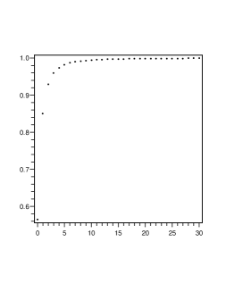
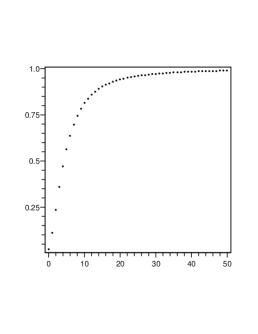
Figure 1: The function $\frac{\varepsilon_{l}(N)}{\beta_{2l}/N^{2l}}$. Left: $l=2$, $n=0$-$30$. Right: $l=16$, $n=0$-$50$.

1.4 Statement of results

In the present paper, we will justify (1.9). In fact, we will prove the following theorem.

      Theorem 1.

For $N=n+3/4$, it holds

$$(-1)^{l+1}\varepsilon_{l}(N)>0$$ (1.10)

for $l=1,2,3,\cdots$ and $n=0,1,2,\cdots$, where $\varepsilon_{l}(N)$ is defined in (1.8), the coefficients $\beta_{2s}$ are determined iteratively in (2.4) below.

The above theorem has direct applications both in asymptotics and sharp bounds. In asymptotic point of view, we can obtain error bounds which in a sense are optimal. To be precise, we have the following.

      Theorem 2.

The error due to truncation of (1.5) is bounded in absolute value by, and of the same sign as, the first neglected term for all nonnegative $n$. That is,

$$0<(-1)^{l+1}\varepsilon_{l}(N)=\left|\varepsilon_{l}(N)\right|<\frac{\left|\beta_{2l}\right|}{N^{2l}}=\frac{(-1)^{l+1}\beta_{2l}}{N^{2l}}$$ (1.11)

for $l=0,1,2\cdots$ and $n=0,1,2,\cdots$, where $N=n+3/4$.

The error bound in (1.11) is the first neglected term in the asymptotic expansion, and hence is optimal and can not be improved. The inequalities in (1.11) can be derived from Theorem 1 by noticing that $\varepsilon_{l}(N)=\beta_{2l}/N^{2l}+\varepsilon_{l+1}(N)$, as can be seen from (1.8).

Another application of Theorem 1 is the construction of sharp bounds up to arbitrary orders.

      Theorem 3.

For $N=n+3/4$, it holds

$$\ln N+\gamma+4\ln 2+\sum_{s=1}^{2m}\frac{\beta_{2s}}{N^{2s}}<\pi G_{n}<\ln N+\gamma+4\ln 2+\sum_{s=1}^{2k-1}\frac{\beta_{2s}}{N^{2s}}$$ (1.12)

for all $n=0,1,2,\cdots$, $m=1,2,\cdots$, and $k=1,2,\cdots$.

The inequalities in (1.12) are understood as sharp bounds on both sides up to arbitrary orders. In a sense, the bounds are optimal and can not be improved.

The first few coefficients $\beta_{2s}$ are listed in Table 1, as can be evaluated via (2.4).

$\beta_{2}$	$\beta_{4}$	$\beta_{6}$	$\beta_{8}$	$\beta_{10}$	$\beta_{12}$	$\beta_{14}$
$\frac{11}{192}$	$\frac{-1541}{122880}$	$\frac{63433}{8257536}$	$\frac{-9199901}{1006632960}$	$\frac{317959723}{17716740096}$	$\frac{-14849190321163}{281406257233920}$	$\frac{717209117969}{3298534883328}$

Table 1: The first few $\beta_{2s}$, $s=1,2,\cdots,7$.

2 Proof of Theorem 1

The proof is based on the difference equation (1.6) and an approximation of the coefficients $\beta_{2s}$. To justify Theorem 1, several lemmas are stated, and all, except one, are proved in the present section. While the validity of Lemma 2 is the objective of the next section.

2.1 The coefficients $\beta_{s}$ in (1.5)

Write the difference equation (1.6) in the symmetrical form

$$\left(1+\frac{1}{4N}\right)^{2}w(N+1)-\left(2+\frac{1}{8N^{2}}\right)w(N)+\left(1-\frac{1}{4N}\right)^{2}w(N-1)=0,$$ (2.1)

in which $N=n+\frac{3}{4}$ for $n=0,1,2,\cdots$. As mentioned earlier and as in the previous paper [8], the Landau constants $w(N)=G_{n}$ solves (2.1), having an asymptotic expansion

$$\pi G_{n}\sim\ln N+\gamma+4\ln 2+\sum^{\infty}_{s=1}\frac{\beta_{s}}{N^{s}},$$ (2.2)

and the coefficients are determined by a formal substitution of (2.2) into (2.1); see Wong and Li [17]. The following result then follows:

      Lemma 1.

For $N=n+\frac{3}{4}$, the coefficients $\beta_{s}$ in expansion (2.2) fulfill

$$\beta_{2k+1}=0,~{}~{}k=0,1,2,\cdots,$$ (2.3)

and

$$\beta_{2k}=\frac{-1}{4k^{2}}\left(d_{k-1,k+1}\beta_{2k-2}+d_{k-2,k+1}\beta_{2k-4}+\cdots+d_{1,k+1}\beta_{2}-d_{0,k+1}\right),~{}~{}k=1,2,\cdots,$$ (2.4)

where $d_{j,j+1}=4j^{2}$ for $j=1,2,\cdots$,

$$d_{j,s}=\frac{(2s+2j-2)\;(2s-2)!}{(2s-2j)!\;(2j-1)!}+\frac{(2s-3)!}{8(2s-2j-2)!\;(2j-1)!}~{}~{}\mbox{for}~{}~{}s\geq j+2,$$ (2.5)

and

$$d_{0,s}=\left(\frac{1}{s}-\frac{1}{2s-1}\right)+\frac{1}{16(s-1)},~{}~{}s=2,3,\cdots.$$ (2.6)

In addition, it holds

$$\beta_{2k}=(-1)^{k+1}\left|\beta_{2k}\right|,~{}~{}k=1,2,\cdots.$$ (2.7)

Part of this lemma ( (2.3) and (2.7) ) has been proved in Nemes’ recent paper [10]. Part of it, namely (2.3), and an equivalent form of (2.4), has been proved in our earlier paper [8]. Following Wong and Li [17], (2.3) and (2.4) can be justified by substituting (2.2) into (2.1), expanding both sides in formal power series of $1/N$, and equalizing the coefficients of the same powers.

It is readily seen that all $d_{j,s}>0$ for $l\geq 1$ and $s\geq l+1$, and $d_{0,s}>0$ for $s\geq 2$.

2.2 Analysis of $R_{l}(N)$

Here,

$$R_{l}(N)=\left(1+\frac{1}{4N}\right)^{2}\varepsilon_{l}(N+1)-\left(2+\frac{1}{8N^{2}}\right)\varepsilon_{l}(N)+\left(1-\frac{1}{4N}\right)^{2}\varepsilon_{l}(N-1),$$ (2.8)

with the error term $\varepsilon_{l}(N)$ being given in (1.8), and $N=n+3/4$.

There are several facts worth mentioning. It is readily seen from (1.8) that $\pi G_{n}-(\gamma+4\ln 2)$ satisfies the difference equation (2.1), and can then be removed from $R_{l}(N)$ in (2.8). If we write $x=1/N$, then the logarithmic singularity at $x=0$ is also cancelled in $R_{l}(N)$. Therefore, each $R_{l}(N)$ is an analytic function in $x$ for $|x|<1$. Hence the asymptotic expansion for $R_{l}(N)$, in descending powers of $N$, is actually a convergent Taylor expansion in $x$,

$$R_{l}(N)=\sum_{s=l+1}^{\infty}r_{l,s}x^{2s},~{}~{}|x|<1,$$ (2.9)

where

$$r_{l,s}=-\left(d_{l-1,s}\beta_{2l-2}+d_{l-2,s}\beta_{2l-4}+\cdots+d_{1,s}\beta_{2}-d_{0,s}\right)$$ (2.10)

for $s\geq l+1$, with the leading coefficient $r_{l,l+1}=4l^{2}\beta_{2l}$; cf. (2.4).

For later use, we estimate the ratio of the consecutive coefficients $\beta_{2s}$. To this end, we introduce a sequence of positive constants

$$\rho_{0}=1,~{}~{}\mbox{and}~{}\rho_{l}=\frac{(-1)^{l+1}\beta_{2l}}{(2l-1)!},~{}~{}l=1,2,\cdots.$$ (2.11)

We shall use the following lemma and leave its proof to Section 3 below.

      Lemma 2.

It holds

$$\rho_{k}/\rho_{k+1}\leq\frac{44}{9}\pi^{2}$$ (2.12)

for $k=0,1,2,\cdots$.

Now we proceed to analyze $R_{l}(N)$ (sometimes denoted by $R_{l}(x)$, understanding that $x=1/N$), so as to show that $R_{l}(x)/\beta_{2l}\geq 0$ for $x\in[0,1)$. More precisely, we prove a much stronger result, as follows:

      Lemma 3.

For $l=1,2,\cdots$ and $N=n+3/4$ with $n=1,2,\cdots$, we have

$$(-1)^{l+1}r_{l,s}>0,~{}~{}s\geq l+1,$$ (2.13)

where $r_{l,s}$ are given in (2.9) and (2.10).

Proof: The lemma can be proved by using induction with respect to $l$. Initially, we have

$$R_{1}(N)=\sum_{s=2}^{\infty}d_{0,s}x^{2s}.$$

Since $d_{0,s}>0$ for $s=2,3,\cdots$; cf. (2.6), we see that (2.13) holds for $l=1$.

In view of the fact that $\beta_{2}=\frac{11}{192}$; cf. Table 1, it is readily verified that

$$R_{2}(N)=\sum_{s=3}^{\infty}r_{2,s}x^{2s}=\sum_{s=3}^{\infty}\left(-\frac{11}{192}d_{1,s}+d_{0,s}\right)x^{2s},$$

with all coefficients $r_{2,s}$ being negative. Indeed, in view of (2.5) and (2.6), we have

$$r_{2,s}=-\frac{11}{192}\left(2s+\frac{2s-3}{8}\right)+\left[\left(\frac{1}{s}-\frac{1}{2s-1}\right)+\frac{1}{16(s-1)}\right]<-\frac{11}{192}\cdot(2s)+\frac{1}{s}<0$$

for $s\geq 3$. Thus (2.13) holds for $l=2$.

Similarly, we can verify (2.13) for $l=3$, recalling that $\beta_{4}=-\frac{1541}{122880}$; cf. Table 1.

Assume that for $l\leq k$, it holds $(-1)^{l+1}r_{l,s}>0$ for $s\geq l+1$. From (2.10), we can write

$$(-1)^{k+3}r_{k+2,s}=(-1)^{k+1}r_{k,s}+(-1)^{k}\left(d_{k+1,s}\beta_{2k+2}+d_{k,s}\beta_{2k}\right)$$ (2.14)

for $s\geq k+3$. To show that (2.13) is valid for $l=k+2$, it suffices to show that

$$(-1)^{k}\left(d_{k+1,s}\beta_{2k+2}+d_{k,s}\beta_{2k}\right)>0$$

for $s\geq k+4$ since the validity of (2.13) for $(l,s)=(k+2,k+3)$ is trivial. This is equivalent to show that

$$c_{k+1,s}-c_{k,s}\rho_{k}/\rho_{k+1}=\frac{(-1)^{k}\left(d_{k+1,s}\beta_{2k+2}+d_{k,s}\beta_{2k}\right)}{8(s-1)^{2}\;(2s-3)!\;\rho_{k+1}}>0,$$ (2.15)

where $\rho_{k}>0$ is defined in (2.11), and $c_{k,s}=\frac{(2k-1)!d_{k,s}}{8(s-1)^{2}(2s-3)!}$; cf. (3.2) below. In view of (2.5), we may write

$$c_{k,s}=\left\{\frac{1}{2(2s-2k)!}+\frac{k}{2(s-1)(2s-2k)!}\right\}+\left\{\frac{1}{64(s-1)^{2}(2s-2k-2)!}\right\}:=A+B.$$

For $k\geq 1$ and $s-k\geq 4$, we have

$$c_{k+1,s}\geq(2s-2k-1)(2s-2k)A+(2s-2k-3)(2s-2k-2)B\geq 56A+30B>\frac{478}{9}c_{k,s}.$$

The last inequality holds since $A>8B$.

From (2.12) in Lemma 2, it is readily verified that

$$\frac{478}{9}>\frac{44}{9}\pi^{2}\geq\frac{\rho_{k}}{\rho_{k+1}}$$

for $k\geq 1$. Then (2.15) holds for $s\geq k+4$, and it follows that $(-1)^{k}\left(d_{k+1,s}\beta_{2k+2}+d_{k,s}\beta_{2k}\right)>0$ for $s\geq k+4$. Accordingly, from (2.14) we see that (2.13) holds for $l=k+2$. This completes the proof of Lemma 3.

2.3 Proof of Theorem 1

Now Lemma 3 implies that $(-1)^{l+1}R_{l}(N)>0$ for all $l$ and all $N=n+3/4$.

To show that $\tilde{\varepsilon}_{l}(N):=(-1)^{l+1}\varepsilon_{l}(N)>0$ for all $N$, we note first that $\tilde{\varepsilon}_{l}(N)=\frac{|\beta_{2l}|}{N^{2l}}\left\{1+O\left(\frac{1}{N^{2}}\right)\right\}$ as $N\rightarrow+\infty$. Hence $\tilde{\varepsilon}_{l}(N)>0$ for $N$ large enough. Now assume that (1.10) is not true. Then there exists a finite $M$ defined as

$$M=\max\{N=n+3/4:~{}n\in\mathbb{Z}~{}\mbox{and}~{}\tilde{\varepsilon}_{l}(N)\leq 0\},$$

so that $M-3/4$ is a positive integer and $\tilde{\varepsilon}_{l}(M)\leq 0$, while $\tilde{\varepsilon}_{l}(M+1),\tilde{\varepsilon}_{l}(M+2),\cdots>0$. For simplicity, we denote $a_{N}=(1+\frac{1}{4N})^{2}$ and $b_{N}=(1-\frac{1}{4N})^{2}$. From (2.8) we have

$$a_{M+1}\tilde{\varepsilon}_{l}(M+2)=(a_{M+1}+b_{M+1})\tilde{\varepsilon}_{l}(M+1)+b_{M+1}\left(-\tilde{\varepsilon}_{l}(M)\right)+(-1)^{l+1}R_{l}(M+1).$$

The later terms on the right-hand side are non-negative, hence we obtain

$$a_{M+1}\tilde{\varepsilon}_{l}(M+2)\geq\left(a_{M+1}+b_{M+1}\right)\tilde{\varepsilon}_{l}(M+1),$$

which implies that

$$\tilde{\varepsilon}_{l}(M+2)>\tilde{\varepsilon}_{l}(M+1).$$ (2.16)

Using (2.8) again for $N=M+2$, we have

$$a_{M+2}\tilde{\varepsilon}_{l}(M+3)\geq(a_{M+2}+b_{M+2})\tilde{\varepsilon}_{l}(M+2)-b_{M+2}\tilde{\varepsilon}_{l}(M+1).$$

A combination of the previous two inequalities gives

$$\tilde{\varepsilon}_{l}(M+3)>\tilde{\varepsilon}_{l}(M+2).$$ (2.17)

In general, we obtain

$$\tilde{\varepsilon}_{l}(M+k+1)>\tilde{\varepsilon}_{l}(M+k)$$ (2.18)

by induction. From the equalities in (2.16), (2.17) and (2.18), we conclude that

$$\tilde{\varepsilon}_{l}(M+k)>\tilde{\varepsilon}_{l}(M+1)$$ (2.19)

for all $k\geq 2$. Recalling that $\tilde{\varepsilon}_{l}(N)=O(N^{-2l})$ for $N\rightarrow\infty$, letting $k\rightarrow\infty$ will give $\tilde{\varepsilon}_{l}(M+1)\leq 0$. This contradicts the definition of $M$. Thus we have proved Theorem 1.

3 Proof of Lemma 2

The idea is simple: to approximate the coefficients $\beta_{2s}$, and then to work out the ratio $\beta_{2s}/\beta_{2s+2}$. Yet the procedure is complicated.

A brief outline of the proof is as follows: In Section 3.1, we bring in an ordinary differential equation (3.10) with a specific analytic solution $v(z)$, of which $\rho_{k}=\frac{(-1)^{k+1}\beta_{2k}}{(2k-1)!}$ are coefficients of the Maclaurin expansion. The function $v(z)$ is then extended, in Section 3.2, and via the hypergeometric functions, to a function analytic in the cut-strip $\{z~{}|~{}-4\pi<\mathop{\rm Re}\nolimits z<4\pi,~{}z\not\in\{(-\infty,-2\pi]\cup[2\pi,+\infty)\}\}$. An integral representation is then obtained by using the Cauchy integral formula, and the integration path is deformed based on the analytic continuation procedure. In Section 3.3, the integral is spilt, approximated, and estimated, and hence bounds for $\rho_{k}$ on both sides are established in (3.25) for all $k\geq 10$. Eventually, in Section 3.4, an upper bound for $\rho_{k}/\rho_{k+1}$ is obtained for all non-negative integer $k$.

3.1 Differential equation

In terms of $\rho_{s}$ defined in (2.11), namely, $\rho_{0}=1$ and $\rho_{l}=\frac{(-1)^{l+1}\beta_{2l}}{(2l-1)!}$ for $l=1,2,\cdots$, formula (2.4) can be written as

$$c_{l,l+1}\rho_{l}-c_{l-1,l+1}\rho_{l-1}+\cdots+(-1)^{k}c_{l-k,l+1}\rho_{l-k}+\cdots+(-1)^{l-1}c_{1,l+1}\rho_{1}+(-1)^{l}c_{0,l+1}\rho_{0}=0$$ (3.1)

for $l=1,2,\cdots$, where $c_{l,l+1}=\frac{1}{2!}$, and

$$c_{l-k,l+1}=\frac{(2l-2k-1)!}{(2l-1)!}\frac{d_{l-k,l+1}}{2d_{l,l+1}}=\frac{1}{2(2k+2)!}+\frac{l-k}{2l(2k+2)!}+\frac{1}{64l^{2}\cdot(2k)!}$$ (3.2)

for $k=1,2,\cdots l-1$ and $l=1,2,\cdots$. It can be verified from (2.6) that $c_{0,l+1}=\frac{d_{0,l+1}}{8l^{2}(2l-1)!}$ also takes the same form, that is, (3.2) is also valid for $k=l$, $l=1,2,\cdots$.

The idea now is to approximate $\rho_{s}$, and then to estimate the ratio $\rho_{s}/\rho_{s+1}$.

Taking $l=1,2,\cdots$ in (3.1), we have

$$\begin{array}[]{l}a_{1}:=c_{1,2}\rho_{1}-c_{0,2}\rho_{0}=0,\\[5.69046pt] a_{2}:=c_{2,3}\rho_{2}-c_{1,3}\rho_{1}+c_{0,3}\rho_{0}=0,\\[5.69046pt] a_{3}:=c_{3,4}\rho_{3}-c_{2,4}\rho_{2}+c_{1,4}\rho_{1}-c_{0,4}\rho_{0}=0,\\[5.69046pt] \cdots\cdots.\end{array}$$

Summing up $\sum^{\infty}_{s=1}a_{s}x^{2s}$ gives

$$\rho_{0}\left(-c_{0,2}x^{2}+c_{0,3}x^{4}-c_{0,4}x^{6}+\cdots\right)+\sum^{\infty}_{k=1}\rho_{k}x^{2k}\sum^{\infty}_{s=1}(-1)^{s-1}c_{k,k+s}x^{2s-2}=0.$$ (3.3)

In view of (3.2), it is readily verified by summing up the series that

$$-c_{0,2}x^{2}+c_{0,3}x^{4}-c_{0,4}x^{6}+\cdots=-\frac{1}{4}+\frac{h(x)}{2}-\int^{x}_{0}\frac{dt_{1}}{t_{1}}\int^{t_{1}}_{0}\frac{th(t)dt}{16},$$ (3.4)

where

$$h(x):=\frac{1-\cos x}{x^{2}}.$$

Also we have, for $k=1,2,\cdots$,

$$\sum^{\infty}_{s=1}(-1)^{s-1}c_{k,k+s}x^{2s-2}=\frac{h(x)}{2}+\frac{k}{x^{2k}}\int^{x}_{0}t^{2k-1}h(t)dt-\frac{1}{x^{2k}}\int^{x}_{0}\frac{dt_{1}}{t_{1}}\int^{t_{1}}_{0}\frac{t^{2k+1}h(t)dt}{16}.$$ (3.5)

Substituting (3.4) and (3.5) into (3.3), we obtain an equation

$$-\frac{1}{4}+\frac{1}{2}h(x)u(x)+\int^{x}_{0}\frac{1}{2}h(t)u^{\prime}(t)dt-\int^{x}_{0}\frac{dt_{1}}{t_{1}}\int^{t_{1}}_{0}\frac{t}{16}h(t)u(t)dt=0,$$ (3.6)

where

$$u(x):=\sum^{\infty}_{k=0}\rho_{k}x^{2k}.$$ (3.7)

      Remark 1.

The existence of $u(x)$ defined above and the validity of (3.3) can be justified by showing that $\left|\rho_{k}\right|\leq M_{0}/\delta^{2k}$ for all positive integers $k$, $M_{0}$ and $\delta$ being positive constants. Indeed, from (3.2) it is readily seen that $\left|c_{l-k,l+1}\right|\leq\frac{1}{(2k)!}$ for $k=1,2,\cdots,l$. Now we assume that $\left|\rho_{k}\right|\leq M_{0}/\delta^{2k}$ for $k<l$, where $\delta$ is small enough such that $2(\cosh\delta-1)<1$. Then, by using (3.1) we have

$$\frac{1}{2}|\rho_{l}|\leq\sum^{l}_{k=1}\left|c_{l-k,l+1}\right||\rho_{l-k}|\leq\sum^{l}_{k=1}\frac{M_{0}\delta^{2k-2l}}{(2k)!}\leq\frac{M_{0}}{\delta^{2l}}\left(\cosh\delta-1\right).$$

Hence we have $\left|\rho_{l}\right|\leq M_{0}/\delta^{2l}$ by induction.

Applying the operator $\displaystyle{\frac{d}{dx}\left(x\frac{d}{dx}\right)}$ to both sides of (3.6), we see that $u(x)$ solves the second order differential equation

$$\left[x\left(\frac{1}{2}h^{\prime}(x)u(x)+h(x)u^{\prime}(x)\right)\right]^{\prime}-\frac{xh(x)u(x)}{16}=0$$ (3.8)

in a neighborhood of $x=0$, with initial conditions $u(0)=1$ and $u^{\prime}(0)=0$.

In the next few steps we derive a representation of $u(x)$ for later use. First, substituting

$$v(x)=\sqrt{h(x)}u(x)=\frac{\sqrt{2}\sin\frac{x}{2}}{x}u(x)$$ (3.9)

into equation (3.8) yields

$$\sin\frac{x}{2}v^{\prime\prime}(x)+\frac{1}{2}\cos\frac{x}{2}v^{\prime}(x)-\frac{1}{16}\sin\frac{x}{2}v(x)=0$$ (3.10)

in a neighborhood of $x=0$, with $v(0)=1/\sqrt{2}$ and $v^{\prime}(0)=0$.

It is shown in Remark 1 that $u(x)$ is analytic at the origin. So is $v(x)$; cf. (3.9). What is more, near $x=0$, the function $v(x)$ can be represented as a hypergeometric function. Indeed, a change of variable

$$t=\frac{1-\cos x}{2}=\sin^{2}\frac{x}{2}$$

turns the equation into the hypergeometric equation

$$t(1-t)\frac{d^{2}v}{dt^{2}}+\left(1-\frac{3}{2}t\right)\frac{dv}{dt}-\frac{1}{16}v=0.$$ (3.11)

Taking the initial conditions into account, it is easily verified that

$$v(x)=\frac{1}{\sqrt{2}}F\left(\frac{1}{4},\frac{1}{4};1;\sin^{2}\frac{x}{2}\right)=\frac{1}{\sqrt{2}}F\left(\frac{1}{2},\frac{1}{2};1;\sin^{2}\frac{x}{4}\right),$$ (3.12)

initially at $x=0$, and then analytically extended elsewhere; cf. [13, (15.2.1)]. The second equality follows from a quadratic hypergeometric transformation; see [13, (15.8.18)].

3.2 Analytic continuation

Well-known formulas for hypergeometric functions include

$$F(a,b;c;t)=\frac{\Gamma(c)}{\Gamma(b)\Gamma(c-b)}\int^{1}_{0}s^{b-1}(1-s)^{c-b-1}(1-st)^{-a}ds$$ (3.13)

for $t\in\mathbb{C}\backslash[1,+\infty)$ as $\mathop{\rm Re}\nolimits c>\mathop{\rm Re}\nolimits b>0$; cf. [13, (15.6.1)], which extends the hypergeometric function to a single-valued analytic function in the cut-plane.

Now we proceed to consider (3.10) with complex variable $z$. It is worth noting that the solution $v(z)$ we seek is an even function. So we restrict ourselves to its analytic continuation on the right-half plane $\mathop{\rm Re}\nolimits z>0$. To this aim, we define

$$f(z)=F\left(\frac{1}{2},\frac{1}{2};1;\sin^{2}\frac{z}{4}\right)~{}~{}\mbox{for}~{}\mathop{\rm Re}\nolimits z\in(-2\pi,2\pi)\cup(2\pi,6\pi).$$ (3.14)

We see that $t=\sin^{2}\frac{z}{4}$ maps the strip $-2\pi<\mathop{\rm Re}\nolimits z<2\pi$ duplicately and analytically onto the cut-plane $t\in\mathbb{C}\backslash[1,+\infty)$. The same is true for $2\pi<\mathop{\rm Re}\nolimits z<6\pi$. Hence from (3.12) we have the analytic continuation $v(z)=f(z)$ for $-2\pi<\mathop{\rm Re}\nolimits z<2\pi$. Moreover, from (3.14) it is readily seen that the function $f(z)$, defined and analytic in the disjoint strips, satisfies

$$f(z)=f(z-4\pi)~{}~{}\mbox{for}~{}~{}\mathop{\rm Re}\nolimits z\in(2\pi,6\pi).$$

Careful treatment should be brought in here, since there is a logarithmic singularity of $v(z)$ at the boundary point $z=2\pi$, as we will see later, and as can be seen from the equation (3.10): $z=2\pi$ is one of the nearest regular singularities, and the indicial equation has a double root $0$ there.

Next, we extend the domain of analyticity of $v(z)$ beyond the vertical line $\mathop{\rm Re}\nolimits z=2\pi$. To do so, we recall the jump along the branch cut of the hypergeometric function

$$F(a,b;c;x+i0)-F(a,b;c;x-i0)=\frac{2\pi i\Gamma(c)}{\Gamma(a)\Gamma(b)}\frac{(x-1)^{c-a-b}}{\Gamma(c-a-b+1)}F(c-a,c-b;c-a-b+1;1-x)$$ (3.15)

for $x>1$; see [13, (15.2.2)-(15.2.3)].

Applying (3.15) to $f(z)$ defined in (3.14), a careful calculation yields

$$f(2\pi-0+iy)-f(2\pi+0+iy)=2if(iy)~{}~{}\mbox{for}~{}~{}y=\mathop{\rm Im}\nolimits z>0,$$

where use has been made of the fact that $t=\sin^{2}\frac{2\pi-0+iy}{4}$, $y=\mathop{\rm Im}\nolimits z>0$ corresponds to the upper edge of $[1,\infty)$, while $t=\sin^{2}\frac{2\pi+0+iy}{4}=\sin^{2}\frac{-2\pi+0+iy}{4}$, $y=\mathop{\rm Im}\nolimits z>0$ corresponds to the lower edge, and that $t=\sin^{2}\frac{z}{4}$ maps the upper imaginary axis to $(-\infty,0)$. Similarly we have

$$f(2\pi-0+iy)-f(2\pi+0+iy)=-2if(iy)~{}~{}\mbox{for}~{}~{}y=\mathop{\rm Im}\nolimits z<0.$$

Summarizing the above, we have an analytic function in the cut-strip $\{z~{}|~{}0\leq\mathop{\rm Re}\nolimits z<4\pi,~{}z\not\in[2\pi,+\infty)\}$, defined as follows:

$$v(z)=\left\{\begin{array}[]{ll}f(z),&0\leq\mathop{\rm Re}\nolimits z<2\pi,\\[2.84544pt] f(z)+2if(z-2\pi),&2\pi<\mathop{\rm Re}\nolimits z<4\pi,~{}\mathop{\rm Im}\nolimits z>0,\\[2.84544pt] f(z)-2if(z-2\pi),&2\pi<\mathop{\rm Re}\nolimits z<4\pi,~{}\mathop{\rm Im}\nolimits z<0.\end{array}\right.$$ (3.16)

The value at $\mathop{\rm Re}\nolimits z=2\pi$, $\mathop{\rm Im}\nolimits z\not=0$ is obtained by taking limit.

At last, we confirm that there is a logarithmic singularity at $z=2\pi$, a regular singularity of (3.10). Indeed, following the derivation from (3.10) to (3.11), we see that all solutions to (3.10) takes the form

$$Aw_{1}(z)+B\left\{w_{1}(z)\ln\left(\sin^{2}\frac{z}{2}\right)+w_{2}(z)\right\}=Aw_{1}(z)+B\left\{2w_{1}(z)\ln\left(z-2\pi\right)+\tilde{w}_{2}(z)\right\};$$

cf. Wong [16, (2.1.24)], where $w_{2}(z)$ and $\tilde{w}_{2}(z)$ are specific single-valued analytic functions at $z=2\pi$, $A$ and $B$ are constants, and $w_{1}(z)=f(z-2\pi)$ is an analytic solution of (3.10) at $z=2\pi$. The function $v(z)$ in (3.16) is such a solution, and, what is more, with $B=-\frac{1}{\pi}$, as can be seen by comparing the jumps along $(2\pi,3\pi)$. Accordingly, we may write

$$v(z)=v_{A}(z)-\frac{2}{\pi}f(z-2\pi)\ln\left(2\pi-z\right)$$ (3.17)

for $0<\mathop{\rm Re}\nolimits z<4\pi$, with $v_{A}(z)$ being analytic in the strip, and the branch of logarithm being chosen as $\arg(2\pi-z)\in(-\pi,\pi)$.

3.3 Approximation of $\rho_{s}$

Now we are in a position to approximate $\rho_{s}$.

To begin, we mention several known facts.

From (3.16), and that $v(z)$ is even, we know that the function $v(z)$ is now extended analytically to the cut-strip

$$\{z~{}|~{}-4\pi<\mathop{\rm Re}\nolimits z<4\pi,~{}z\not\in\{(-\infty,-2\pi]\cup[2\pi,+\infty)\}\}.$$

Again, from (3.14), (3.16) and (3.17), and that the hypergeometric function $F(a,a;c;t)$ behaviors of the form $O(|t|^{-a}\ln|t|)$ at infinity; see [13, (15.8.8)], we conclude that

$$v(z)=O\left(e^{-\frac{1}{4}|\mathop{\rm Im}\nolimits z|}\ln|\mathop{\rm Im}\nolimits z|\right)$$

as $\mathop{\rm Im}\nolimits z\rightarrow\infty$, holding uniformly in $|\mathop{\rm Re}\nolimits z|\leq 4\pi-\delta$ for arbitrary positive $\delta$. Thus $v(z)$ displays an exponentially small decay at infinity in each sub-strip.

Hence, we can derive from (3.7) and (3.9) that

$$\rho_{k}=\frac{1}{2\pi i}\oint z^{-2k-1}u(z)dz=\frac{1}{\sqrt{2}\pi i}\oint\frac{\frac{z}{2}}{\sin\frac{z}{2}}\frac{v(z)dz}{z^{2k+1}}=\frac{1}{\sqrt{2}\pi i}\int_{\Gamma}\frac{\frac{z}{2}}{\sin\frac{z}{2}}\frac{v(z)dz}{z^{2k+1}},$$ (3.18)

where initially the integration path is a small circle encircling the origin, and then being deformed to the contour $\Gamma$ illustrated in Figure 2.

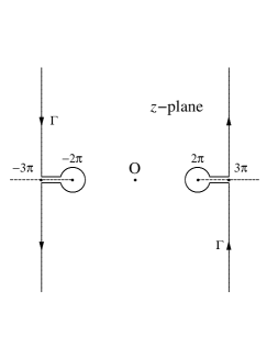
Figure 2: The deformed contour $\Gamma$: the oriented curve.

From the symmetry property of $v(z)$, we need only evaluate and estimate the integral on the right-half of $\Gamma$. We split the integral in (3.18) into three integrals, namely,

$$\frac{\pi i}{\sqrt{2}}\rho_{k}=\int_{\Gamma_{v}}\frac{\frac{z}{2}}{\sin\frac{z}{2}}\frac{v(z)dz}{z^{2k+1}}+\int_{\Gamma_{l}}\frac{\frac{z}{2}}{\sin\frac{z}{2}}\frac{v_{A}(z)dz}{z^{2k+1}}-\int_{\Gamma_{l}}\frac{\frac{z}{\pi}f(z-2\pi)\ln(2\pi-z)dz}{\sin\frac{z}{2}~{}z^{2k+1}}:=I_{v}+I_{a}+I_{l},$$ (3.19)

where $\Gamma_{v}$ is the right-half vertical part $\mathop{\rm Re}\nolimits z=3\pi$, and $\Gamma_{l}$ is the remaining right-half $\Gamma$, consisting of an circular part around $z=2\pi$, and a pair of horizontal line segments joining the circle with the vertical line; compare Figure 2 for the curves and the orientation.

We will show that the main contribution to $\rho_{k}$, when $k$ is not small, comes from $I_{l}$. Estimates will be obtained with full details. We do the calculation case by case.

Estimating $I_{v}$:

First, we estimate $v(z)$ for $\mathop{\rm Re}\nolimits z=3\pi$. It is readily seen that $t=\sin^{2}\frac{3\pi+iy}{4}=\frac{1-i\sinh y}{2}$ and $\sin^{2}\frac{\pi+iy}{4}=\frac{1+i\sinh y}{2}$, where $y=\mathop{\rm Im}\nolimits z$. Hence

$$\arg\left\{(1-st)^{-\frac{1}{2}}\right\}\in(-\pi/2,0)~{}\mbox{for}~{}y\in(0,\infty),~{}~{}\mbox{and}~{}\left|(1-st)^{-\frac{1}{2}}\right|\leq\left(1-\frac{s}{2}\right)^{-\frac{1}{2}}~{}\mbox{for}~{}0\leq s\leq 1.$$

Accordingly, from (3.13) and (3.14) we have

$$\left|f(3\pi+iy)\right|\leq\frac{1}{\pi}\int^{1}_{0}s^{-\frac{1}{2}}(1-s)^{-\frac{1}{2}}\left(1-s/2\right)^{-\frac{1}{2}}ds:=C_{f,v}=1.1803\cdots~{}~{}\mbox{for}~{}~{}y>0.$$

Noting that $\arg f(3\pi+iy)\in(-\pi/2,0)$ for $y>0$, and that $f(\pi+iy)=\overline{f(3\pi+iy)}$, Substituting all above into (3.16), we have

$$|v(3\pi+iy)|\leq\sqrt{5}\left|f(3\pi+iy)\right|\leq M_{v}:=\sqrt{5}\;C_{f,v}=2.6393\cdots,~{}~{}y>0.$$

Similar argument shows that the equality holds for $y\in\mathbb{R}$.

Hence, we conclude from (3.16) and (3.19) that

$$|I_{v}|\leq\frac{1}{2}\int^{\infty}_{-\infty}\frac{|v(3\pi+iy)|\;dy}{\cosh\frac{y}{2}~{}|3\pi+iy|^{2k}}\leq\frac{M_{v}}{2}\frac{1}{(3\pi)^{2k}}\int^{\infty}_{-\infty}\frac{dy}{\cosh\frac{y}{2}}=\frac{\pi M_{v}}{(3\pi)^{2k}}=\frac{8.2916\cdots}{(3\pi)^{2k}}.$$ (3.20)

Evaluating $I_{a}$:

This time, $v_{A}(z)$ is analytic in a domain containing $\Gamma_{l}$. It is readily seen that only the simple pole $z=2\pi$ contributes to $I_{a}$. More precisely, applying the residue theorem we have

$$I_{a}=\frac{2\pi iv_{A}(2\pi)}{(2\pi)^{2k}}.$$

Here $v_{A}(2\pi)$ can be obtained by substituting $z=2\pi-\varepsilon$ into (3.16) and (3.17), and taking limit

$$v_{A}(2\pi)=\lim_{\varepsilon\rightarrow 0^{+}}\left\{\frac{1}{\pi}\int^{1}_{0}s^{-\frac{1}{2}}(1-s)^{-\frac{1}{2}}(1-st)^{-\frac{1}{2}}ds+\frac{2}{\pi}f(-\varepsilon)\ln\varepsilon\right\},$$

where $t=\sin^{2}\frac{z}{4}=\cos^{2}\frac{\varepsilon}{4}$; cf. (3.13) and (3.14).

A careful calculation leads to

$$v_{A}(2\pi)=\frac{1}{\pi}\int^{1}_{0}\frac{s^{-\frac{1}{2}}-1}{1-s}ds+\frac{1}{\pi}\int^{1}_{0}\frac{s^{-\frac{1}{2}}-1}{1-s}ds+\frac{4}{\pi}\ln 2=\frac{8}{\pi}\ln 2.$$ (3.21)

Indeed, (3.21) can be derived as follows:

$$\frac{1}{\pi}\int^{1}_{0}\left(s^{-\frac{1}{2}}-1\right)(1-s)^{-\frac{1}{2}}(1-st)^{-\frac{1}{2}}ds\longrightarrow\frac{1}{\pi}\int^{1}_{0}\frac{s^{-\frac{1}{2}}-1}{1-s}ds~{}~{}\mbox{as}~{}~{}t\rightarrow 1^{-}$$

by applying the dominated convergence theorem. Also,

$$\frac{1}{\pi}\int^{1}_{0}(1-s)^{-\frac{1}{2}}(1-st)^{-\frac{1}{2}}ds=\frac{1}{\pi}\int^{1}_{0}\frac{\tau^{-\frac{1}{2}}}{1-t\tau}d\tau$$

by making change of variable $\tau=\frac{1-s}{1-ts}$. Finally,

$$\frac{1}{\pi}\int^{1}_{0}\left\{s^{-\frac{1}{2}}-1\right\}\frac{1}{1-ts}ds\longrightarrow\frac{1}{\pi}\int^{1}_{0}\frac{s^{-\frac{1}{2}}-1}{1-s}ds~{}~{}\mbox{as}~{}~{}t\rightarrow 1^{-}$$

by applying the dominated convergence theorem one more time. For $t<1$, it further holds

$$\frac{1}{\pi}\int^{1}_{0}\frac{1}{1-ts}ds=-\frac{1}{\pi t}\ln(1-t).$$

Adding up all these gives (3.21). Thus we have

$$I_{a}=\frac{16\ln 2}{(2\pi)^{2k}}i=\frac{11.0903\cdots}{(2\pi)^{2k}}i.$$ (3.22)

Evaluating $I_{l}$:

Now we turn to the last integral $I_{l}$ in (3.19). First, we observe that $\displaystyle{\frac{f(z-2\pi)}{\sin\frac{z-2\pi}{2}}-\frac{f(0)}{\frac{z-2\pi}{2}}}$ is analytic in the strip $\mathop{\rm Re}\nolimits z\in(0,4\pi)$. Hence the circular part of $\Gamma_{l}$ collapses in the following integral to give

$$\frac{1}{\pi}\int_{\Gamma_{l}}\left\{\frac{f(z-2\pi)}{\sin\frac{z-2\pi}{2}}-\frac{f(0)}{\frac{z-2\pi}{2}}\right\}\frac{\ln(2\pi-z)}{z^{2k}}dz=-2i\int_{2\pi}^{3\pi}\left\{\frac{f(z-2\pi)}{\sin\frac{z-2\pi}{2}}-\frac{f(0)}{\frac{z-2\pi}{2}}\right\}\frac{dz}{z^{2k}}.$$

Accordingly we have

$$\left|\frac{1}{\pi}\int_{\Gamma_{l}}\left\{\frac{f(z-2\pi)}{\sin\frac{z-2\pi}{2}}-\frac{f(0)}{\frac{z-2\pi}{2}}\right\}\frac{\ln(2\pi-z)}{z^{2k}}dz\right|\leq\frac{4\pi M_{f}}{2k-1}\frac{1}{(2\pi)^{2k}},$$

where

$$M_{f}\geq\max_{2\pi\leq z\leq 3\pi}\left|\frac{f(z)}{\sin\frac{z-2\pi}{2}}-\frac{f(2\pi)}{\frac{z-2\pi}{2}}\right|.$$

We give a rough estimate for this maximum value. Recalling that $f(z)=F\left(\frac{1}{2},\frac{1}{2};1;\sin^{2}\frac{z}{4}\right)$ and $f(0)=1$, noting that the Maclaurin expansion of $F\left(\frac{1}{2},\frac{1}{2};1;t\right)$ has all positive coefficients (cf. [13, (15.2.1)]), and that $\frac{d}{dt}\left(\frac{F\left(\frac{1}{2},\frac{1}{2};1;t\right)-1}{\sqrt{t}}\right)>0$ for $t\in(0,1)$ via term-by-term differentiation, we see that $\frac{f(z-2\pi)-1}{\sin\frac{z-2\pi}{2}}=\frac{1}{2\cos\frac{z-2\pi}{4}}\frac{F\left(\frac{1}{2},\frac{1}{2};1;t\right)-1}{\sqrt{t}}$ is monotone increasing for $2\pi<z\leq 3\pi$, or correspondingly, $t=\sin^{2}\frac{z-2\pi}{4}\in(0,1/2]$. Therefore, we have

$$0<\frac{f(z-2\pi)-1}{\sin\frac{z-2\pi}{2}}\leq F\left(\frac{1}{2},\frac{1}{2};1;\frac{1}{2}\right)-1=\frac{\sqrt{\pi}}{\Gamma(3/4)\Gamma(3/4)}-1;$$

see [13, (15.4.28)]. Also, one has

$$0<\frac{1}{\sin x}-\frac{1}{x}=\frac{x-\sin x}{x\sin x}\leq\frac{x^{3}}{6x\sin x}\leq\frac{\pi^{2}}{24}~{}~{}\mbox{for}~{}~{}0<x\leq\frac{\pi}{2}.$$

Hence an appropriate choice of $M_{f}$ is

$$M_{f}=\frac{\sqrt{\pi}}{\Gamma(3/4)\Gamma(3/4)}-1+\frac{\pi^{2}}{24}=0.5915\cdots.$$

We proceed to evaluate the crucial part

$$\frac{2}{\pi}\int_{\Gamma_{l}}\frac{\ln(2\pi-z)}{z-2\pi}\frac{dz}{z^{2k}},$$

of which the integrand has a pole $z=2\pi$, coinciding with the logarithmic singularity. To treat such kind of singularities, we appeal to the idea of Wong and Wyman [18].

For simplicity we re-scale the variable $\tau=\frac{z-2\pi}{2\pi}$, which turns the integral into

$$\frac{2}{\pi(2\pi)^{2k}}\int_{\frac{1}{2}}^{(0-)}\frac{\ln(2\pi)+\ln(-\tau)}{\tau}\frac{d\tau}{e^{2k\ln(1+\tau)}}=-\frac{4i\ln 2\pi}{(2\pi)^{2k}}+\frac{2}{\pi(2\pi)^{2k}}\int_{\frac{1}{2}}^{(0-)}\frac{\ln(-\tau)}{\tau}\frac{d\tau}{e^{2k\ln(1+\tau)}},$$

where the integration path starts and ends at $\tau=\frac{1}{2}$, and encircles the origin clockwise: the loop is a re-scaled version of $\Gamma_{l}$. The branch of $\ln(1+\tau)$ is chosen so that $\ln(1+\tau)>0$ for $\tau>0$.

To extract the main contribution, we further split the exponent in the integrand. Indeed, we see that

$$\left|\frac{2}{\pi(2\pi)^{2k}}\int_{\frac{1}{2}}^{(0-)}\frac{e^{2k(\tau-\ln(1+\tau))}-1}{\tau}e^{-2k\tau}\ln(-\tau)d\tau\right|\leq\frac{2}{(2\pi)^{2k}}\max_{0\leq\tau<1/2}\left|\varphi(\tau)\right|\leq\frac{2M_{\varphi}}{(2\pi)^{2k}},$$

where the function

$$\varphi(\tau)=\frac{e^{2k(\tau-\ln(1+\tau))}-1}{\tau}e^{-2k\tau}$$

is analytic in a neighborhood of $[0,1/2]$, thus the integration path collapses to the lower and upper edges of $[0,1/2]$, and its bound $M_{\varphi}$ can be obtained by noticing that

$$0\leq\tau-\ln(1+\tau)\leq\frac{\tau^{2}}{2}~{}~{}\mbox{for}~{}~{}\tau>0,~{}~{}~{}\mbox{and}~{}~{}-\ln(1+\tau)\leq-\frac{2}{3}\tau~{}~{}\mbox{for}~{}~{}0\leq\tau\leq\frac{1}{2}.$$

Now for $0\leq\tau\leq\frac{1}{\sqrt{k}}$, one has

$$0\leq\varphi(\tau)\leq\frac{e^{k\tau^{2}}-1}{\tau}e^{-2k\tau}\leq(e-1)(k\tau)e^{-2(k\tau)}\leq\frac{e-1}{2e}.$$

While for $\frac{1}{\sqrt{k}}\leq\tau\leq\frac{1}{2}$,

$$0\leq\varphi(\tau)\leq\frac{e^{-2k\ln(1+\tau)}}{\tau}\leq\frac{e^{-\frac{4}{3}k\tau}}{\tau}\leq\left.\frac{e^{-\frac{4}{3}k\tau}}{\tau}\right|_{\tau=\frac{1}{\sqrt{k}}}=\sqrt{k}e^{-\frac{4}{3}\sqrt{k}}\leq\frac{3}{4e}.$$

Thus we may chose

$$M_{\varphi}=\max\left(\frac{e-1}{2e},\frac{3}{4e}\right)=\frac{e-1}{2e},$$

which does not depend on $k$.

The remaining piece would turn out to be of the most significance. Indeed, a change of variable $s=2k\tau$ makes

$$\begin{array}[]{rl}\displaystyle{\frac{2}{\pi(2\pi)^{2k}}\int_{\frac{1}{2}}^{(0-)}\frac{\ln(-\tau)}{\tau}e^{-2k\tau}d\tau}&=\displaystyle{\frac{2}{\pi(2\pi)^{2k}}\int_{k}^{(0-)}\frac{\ln(-s)-\ln 2k}{s}e^{-s}ds}\\[11.38092pt] &=\displaystyle{\frac{4i\ln 2k}{(2\pi)^{2k}}+\frac{2}{\pi(2\pi)^{2k}}\int_{k}^{(0-)}\frac{\ln(-s)}{s}e^{-s}ds.}\end{array}$$

The last integral can be approximated by extending the integration path to $\displaystyle{\int_{+\infty}^{(0-)}}$, with an error bounded by $\displaystyle{\frac{4e^{-k}}{k(2\pi)^{2k}}}$. Recalling the integral representation

$$\frac{1}{\Gamma(z)}=\frac{1}{2\pi i}\int^{(0-)}_{+\infty}(-s)^{-z}e^{-s}ds$$

for all finite $z$; cf. [13, (5.9.2)] or Wong and Wyman [18], taking derivative with respect to $z$ and setting $z=1$, we obtain

$$\int^{(0-)}_{+\infty}\frac{\ln(-s)}{s}e^{-s}ds=\frac{2\pi i\Gamma^{\prime}(1)}{\Gamma^{2}(1)}=-2\pi i\gamma,$$

where $\gamma=0.5772\cdots$ is Euler’s constant; see [13, (5.4.12)].

Hence we can write

$$I_{l}=\frac{4i\ln 2k}{(2\pi)^{2k}}+\frac{(-4\gamma-4\ln 2\pi)i+\delta_{l,k}}{(2\pi)^{2k}},$$ (3.23)

with

$$|\delta_{l,k}|\leq\frac{4\pi M_{f}}{2k-1}+2M_{\varphi}+\frac{4e^{-k}}{k}.$$

Now we sum up the calculations and estimations made above. Substituting (3.20), (3.22) and (3.23) into (3.19), we have the approximation

$$\frac{\pi}{\sqrt{2}}\rho_{k}=\frac{4\ln 2k}{(2\pi)^{2k}}+\frac{\left(11.0903\cdots-4\gamma-4\ln 2\pi\right)+\delta_{k}}{(2\pi)^{2k}},$$ (3.24)

with

$$|\delta_{k}|\leq\pi M_{v}\left(\frac{2}{3}\right)^{2k}+\frac{4\pi M_{f}}{2k-1}+2M_{\varphi}+\frac{4e^{-k}}{k}<1.0259$$

for $k\geq 10$. Hence we obtain from (3.24) that

$$\frac{4\ln 2k+0.4041\cdots}{(2\pi)^{2k}}\leq\frac{\pi}{\sqrt{2}}\rho_{k}\leq\frac{4\ln 2k+2.4559\cdots}{(2\pi)^{2k}}$$ (3.25)

for $k\geq 10$.

3.4 The ratio

For $k\geq 10$, it is readily verified that

$$\frac{8}{9}\ln(2k+2)\geq 2.7475\cdots>2.4559-\frac{11}{9}\times 0.4041\cdots.$$

Therefore, it follows from (3.25) that

$$\rho_{k}/\rho_{k+1}\leq\frac{44}{9}\pi^{2}$$

for $k\geq 10$.

It is easily verified that the inequality holds for all $k\geq 0$ by numerical evaluation of the first few $\rho_{k}$ for $k=0,1,\cdots 9$, as can be seen from Table 2.

$k$	$0$	$1$	$2$	$3$	$4$	$5$	$6$	$7$	$8$	$9$
$\rho_{k}/\rho_{k+1}$	17.46	27.41	32.65	35.30	36.67	37.41	37.86	38.15	38.36	38.51
$\frac{44}{9}\pi^{2}$	48.25	48.25	48.25	48.25	48.25	48.25	48.25	48.25	48.25	48.25

Table 2: The first few $\rho_{k}$, $k=0,2,\cdots,9$.

A by-product is that $\rho_{k}/\rho_{k+1}\rightarrow 4\pi^{2}$ as $k\rightarrow\infty$. Another byproduct of (3.25) and Table 2 is that $\rho_{k}>0$ for all $k$, and thus $\beta_{2k}$ having alternative signs, as stated in (2.7).

4 Discussion

We discuss very briefly a conjecture of H. Granath, of which we were not aware until we almost finish writing the present paper. In [5], Granath derives an asymptotic expansion

$$\pi G_{n-1}\sim\ln(16n)+\gamma+\sum_{k=1}^{\infty}\frac{a_{k}}{(16n)^{k}},~{}~{}n\rightarrow\infty,$$ (4.1)

where $a_{k}$ are ‘effectively computable’ constants but not explicitly given, except for the first few. The author shows interest in seeking sharp bounds of arbitrary orders. Indeed, denoting

$$A_{m}(n)=\ln(16n)+\gamma+\sum_{k=1}^{m}\frac{a_{k}}{(16n)^{k}},$$ (4.2)

Granath proves that $A_{5}(n)<\pi G_{n-1}<A_{7}(n)$ and states that $A_{9}(n)<\pi G_{n-1}<A_{11}(n)$, for all positive $n$. It is then conjectured that (the sign in [5, (10)] is apparently wrong)

$$(-1)^{\frac{m(m+1)}{2}}\left(\pi G_{n-1}-A_{m}(n)\right)<0$$ (4.3)

for all $n=1,2,\cdots$ and $m=0,1,2,\cdots$.

The existence of (4.1) has also been justified in [8] and [11]. It is easily seen that in terms of $\beta_{s}$ in (2.3) and (2.4), the coefficients can be written as

$$a_{k}=4^{k}\left[-\frac{1}{k}+\sum^{k}_{s=1}\frac{(k-1)!4^{s}\beta_{s}}{(s-1)!(k-s)!}\right],~{}~{}k=1,2,\cdots;$$ (4.4)

see also [8] for an iterative formula. So far, numerical experiments agree with (4.3). A proof of it might be found either by following the steps, or by using the results, of the present paper.

Then, a natural question arises:

      Question 2.

Considering the general expansion in (1.4), for what $h$ we have the “best” approximation in the sense of Theorem 1 and (4.3)?

The case $h=3/4$ is what we have been dealt with in the present paper. Very likely the expansion (1.4) for $h=1/2$ and $h=1$ would turn out to be the “best”.

As mentioned earlier, the coefficients $\beta_{2s}$ of the expansion (1.5) can be obtained iteratively via (2.4). We complete the paper by giving a couple of alternative representations for $\beta_{2s}$. For example, it can be shown that

$$\beta_{2l}=\frac{(-1)^{l+1}}{2^{2l}(l!)^{2}}\left|\begin{array}[]{cccccc}d_{0,2}&d_{0,3}&\cdots&d_{0,l-1}&d_{0,l}&d_{0,l+1}\\ d_{1,2}&d_{1,3}&\cdots&d_{1,l-1}&d_{1,l}&d_{1,l+1}\\ 0&d_{2,3}&\cdots&d_{2,l-1}&d_{2,l}&d_{2,l+1}\\ \vdots&\vdots&\ddots&\vdots&\vdots&\vdots\\ 0&0&\cdots&d_{l-2,l-1}&d_{l-2,l}&d_{l-2,l+1}\\ 0&0&\cdots&0&d_{l-1,l}&d_{l-1,l+1}\\ \end{array}\right|,~{}~{}~{}l=1,2,\cdots.$$ (4.5)

Indeed, taking $k=1,2,\cdots,l$ in (2.4), we have a linear algebraic system with unknowns $\beta_{2}$, $\beta_{4}$, $\cdots$, $\beta_{2l}$. Solving the system gives (4.5).

Also, a combination of (2.11), (3.12) and (3.18) yields an integral representation

$$\beta_{2l}=\frac{(-1)^{l+1}(2l-1)!}{4\pi i}\oint\frac{z}{\sin\frac{z}{2}}\frac{F\left(1/4,1/4;1;\sin^{2}\frac{z}{2}\right)dz}{z^{2l+1}},~{}~{}l=1,2,\cdots,$$ (4.6)

where the integration path is a small circle encircling the origin counterclockwise. Of course, (3.24) can be interpreted as

$$\beta_{2l}=\frac{(-1)^{l+1}(2l-1)!}{\pi(2\pi)^{2l}}\left\{4\sqrt{2}\ln(2l)+O(1)\right\}$$ (4.7)

for large $l$. Results can be obtained from such approximations. For example, the expansion (1.5) is divergent; compare [5, Theorem 3].

References

- [1] H. Alzer, Inequalities for the constants of Landau and Lebesgue, J. Comput. Appl. Math., 139 (2002), 215-230.
- [2] L. Brutman, A sharp estimate of the Landau constants, J. Approx. Theory, 34 (1982), 217-220.
- [3] D. Cvijović and J. Klinowski, Inequalities for the Landau constants, Math. Slovaca, 50 (2000), 159-164.
- [4] L.P. Falaleev, Inequalities for the Landau constants, Siberian Math. J., 32 (1991), 896-897.
- [5] H. Granath, On inequalities and asymptotic expansions for the Landau constants, J. Math. Anal. Appl., 386 (2012), 738-743.
- [6] M.E.H. Ismail, X. Li and M. Rahman, Landau constants and their -analogues, Anal. Appl., DOI: 10.1142/S0219530514500201.
- [7] E. Landau, Abschätzung der koeffzientensumme einer potenzreihe, Arch. Math. Phys., 21 (1913), 42-50, 250-255.
- [8] Y.-T. Li, S.-Y. Liu, S.-X. Xu and Y.-Q. Zhao, Full asymptotic expansions of the Landau constants via a difference equation approach, Appl. Math. Comput., 219 (2012), 988-995.
- [9] C. Mortici, Sharp bounds of the Landau constants, Math. Comp., 80 (2011), 1011-1018.
- [10] G. Nemes, Proofs of two conjectures on the Landau constants, J. Math. Anal. Appl., 388 (2012), 838-844.
- [11] G. Nemes and A. Nemes, A note on the Landau constants, Appl. Math. Comput., 217 (2011), 8543-8546.
- [12] F.W.J. Olver, Asymptotics and Special Functions, Academic Press, New York, 1974.
- [13] F.W.J. Olver, D.W. Lozier, R.F. Boisvert and C.W. Clark, NIST Handbook of Mathematical Functions, Cambridge University Press, New York, 2010.
- [14] P.N. Shivakumar and R. Wong, Asymptotic expansion of the Lebesgue constants associated with polynomial interpolation, Math. Comp., 39 (1982), 195-200.
- [15] G.N. Watson, The constants of Landau and Lebesgue, Q. J. Math. Oxford Ser., 1 (1930), 310-318.
- [16] R. Wong, Lecture Notes on Applied Analysis, World Scientific, Singapore, 2010.
- [17] R. Wong and H. Li, Asymptotic expansions for second-order linear difference equations, J. Comput. Appl. Math., 41 (1992), 65-94.
- [18] R. Wong and M. Wyman, The method of Darboux, J. Approx. Theory, 10 (1974), 159-171.
- [19] D. Zhao, Some sharp estimates of the constants of Landau and Lebesgue, J. Math. Anal. Appl., 349 (2009), 68-73.