Domain walls and vortices in chiral symmetry breaking

Abstract

We study domain walls and vortices in chiral symmetry breaking in a QCD-like theory with $N$ flavors in the chiral limit. If the axial anomaly is absent, there exist stable Abelian axial vortices winding around the spontaneously broken $U(1)_{\rm A}$ symmetry and non-Abelian axial vortices winding around both the $U(1)_{\rm A}$ and non-Abelian $SU(N)$ chiral symmetries. In the presence of the axial anomaly term, metastable domain walls are present and Abelian axial vortices must be attached by $N$ domain walls, forming domain wall junctions. We show that a domain wall junction decays into $N$ non-Abelian vortices attached by domain walls, implying its metastability. We also show that domain walls decay through the quantum tunneling by creating a hole bounded by a closed non-Abelian vortex.

I Introduction

Domain walls produced at phase transitions are known to cause a conflict with cosmology. When the Universe undergoes a phase transition, domain walls are formed if the order parameter space allows them. These domain walls dominate the energy density of the Universe, which is not acceptable from a cosmological point of view (the domain wall problem). Phase transitions at very high energies ($\sim 10^{16}{\rm GeV}$) are not harmful, since the energy density is diluted by the inflation. However, phase transitions below that scale can be dangerous. It is well known that axion models, which are elegant extensions of the standard model for solving the strong CP problem Peccei:1977hh ; Peccei:1977ur ; Weinberg:1977ma ; Wilczek:1977pj , suffer from this problem if the number of flavors is larger than one Sikivie:1982qv ; Peccei:1977hh ; Peccei:1977ur ; Dine:1981rt .

The chiral phase transition in quantum chromodynamics(QCD) is apparently problematic as pointed out in Ref. Forbes:2000et , since domain walls may be produced at the chiral symmetry breaking Zhang:1997is ; Balachandran:2001qn ; Balachandran:2002je . It is still unclear whether the domain walls actually form or not in the early Universe, because the chiral symmetry breaking is a crossover as a function of temperature rather than a phase transition at zero baryon density. If the crossover is very dull, no production of the domain walls is possible. In contrast, the domain walls are expected to form if the crossover is sharp enough and the chiral condensation rapidly grows. In order to clarify this point, one must examine the relaxation timescales involved, which are beyond the scope of this work. In the latter case, in particular, a junction of three domain walls glued by an Abelian axial vortex was found in Ref. Balachandran:2001qn so that domain wall network would be produced that would make domain walls long-lived. Also, a heavy-ion collider at GSI is designed to achieve a finite baryon density, which may turn the chiral symmetry breaking from a crossover to a sharp transition. In that case, the production of topological defects will be inevitable.

In this paper, we study the (in)stability of domain walls and vortices in chiral symmetry breaking in a QCD-like theory in which we take into account light scalar mesons while ignoring other heavy modes such as vector mesons. We find that domain wall junctions are metastable and decay into separate multiple domain walls edged by non-Abelian axial vortices Balachandran:2002je , which are the fundamental vortex solutions Nitta:2007dp ; Nakano:2007dq ; Eto:2009wu . We show that the decays are possible from a topological point of view and perform numerical simulations of decaying junctions. We next show that domain walls themselves can decay by making use of non-Abelian vortices. In a domain wall, holes whose boundaries are non-Abelian vortices can be excited quantum-mechanically or thermally. We make an estimate of the decay rate.

The same types of topological defects also exist in QCD at high baryon density Eto:2013hoa , where the color-flavor locked phase is realized and the chiral symmetry is spontaneously broken Alford:1997zt ; Alford:1998mk ; Alford:2007xm . The chiral Lagrangian in this case was discussed in Ref. Casalbuoni:1999wu . Therefore, the same discussions in this paper hold also for high-density QCD.

This paper is organized as follows. In Sect. II, we present the Ginzburg-Landau effective theory for the chiral symmetry breaking. In Sect. III, we describe domain walls and vortices. In Sect. IV, we consider composite states of domain walls and vortices in the presence of the axial anomaly term. We numerically construct a three-domain wall junction for three flavor QCD. In Sect. V, we show the instability of the domain wall junction topologically and simulate such a decay numerically. Section VII is devoted to the summary and discussion.

II Ginzburg-Landau effective Lagrangian

The chiral symmetry $SU(N)_{\rm L}\times SU(N)_{\rm R}\times U(1)_{\rm A}$ acts on $N$-flavor left- and right-handed massless chiral fermions $\psi_{{\rm L}i}$ and $\psi_{{\rm R}i}$ as

$$\psi_{{\rm L}i}\to e^{-i\theta_{\rm A}/2}g_{\rm L}\psi_{{\rm L}i},\quad\psi_{{\rm R}i}\to e^{+i\theta_{\rm A}/2}g_{\rm R}\psi_{{\rm R}i},$$

$$\left(e^{i\theta_{\rm A}},g_{\rm L},g_{\rm R}\right)\in U(1)_{\rm A}\times SU(N)_{\rm L}\times SU(N)_{\rm R},$$ (1)

where $U(1)_{\rm A}$ is explicitly broken by the axial anomaly. When chiral condensation occurs,

$$\Sigma_{ij}\sim\left<\bar{\psi}_{{\rm L}i}\psi_{{\rm R}j}\right>\neq 0,$$ (2)

the chiral symmetry is spontaneously broken. Here $\Sigma$ is an $N\times N$ complex matrix scalar field, transforming under the chiral symmetry as

$$\Sigma\to e^{i\theta_{\rm A}}g_{\rm L}^{\dagger}\Sigma g_{\rm R},\qquad\left(e^{i\theta_{\rm A}},g_{\rm L},g_{\rm R}\right)\in U(1)_{\rm A}\times SU(N)_{\rm L}\times SU(N)_{\rm R}.$$ (3)

There is a redundancy in the chiral symmetry acting on the scalar field $\Sigma$. The true symmetry group is written as

$$G=\frac{SU(N)_{\rm L}\times SU(N)_{\rm R}\times U(1)_{\rm A}}{({\mathbb{Z}}_{N})_{\rm L+A}\times({\mathbb{Z}}_{N})_{\rm R+A}}\simeq{SU(N)_{\rm L}\times SU(N)_{\rm R}\times U(1)_{\rm A}\over({\mathbb{Z}}_{N})_{\rm L+R}\times({\mathbb{Z}}_{N})_{\rm L-R+A}},$$ (4)

where the redundant discrete groups are

$$(\mathbb{Z}_{N})_{\rm L+A} : \left(\omega_{N}^{k}{\bf 1}_{N},{\bf 1}_{N},\omega_{N}^{-k}\right)\in SU(N)_{\rm L}\times SU(N)_{\rm R}\times U(1)_{\rm A},$$ (5)

$$(\mathbb{Z}_{N})_{\rm R+A} : \left({\bf 1}_{N},\omega_{N}^{k}{\bf 1}_{N},\omega_{N}^{-k}\right)\in SU(N)_{\rm L}\times SU(N)_{\rm R}\times U(1)_{\rm A},$$ (6)

$$(\mathbb{Z}_{N})_{\rm L+R} : \left(\omega_{N}^{k}{\bf 1}_{N},\omega_{N}^{-k}{\bf 1}_{N},1\right)\in SU(N)_{\rm L}\times SU(N)_{\rm R}\times U(1)_{\rm A},$$ (7)

$$(\mathbb{Z}_{N})_{\rm L-R+A} : \left({\omega_{N}^{k}\bf 1}_{N},\omega_{N}^{k}{\bf 1}_{N},\omega_{N}^{-2k}\right)\in SU(N)_{\rm L}\times SU(N)_{\rm R}\times U(1)_{\rm A},$$ (8)

with $\omega_{N}\equiv e^{i\frac{2\pi}{N}}$ and $k=0,1,\cdots,N-1$.

The generic Ginzburg-Landau effective Lagrangian $\Sigma$ in the chiral limit can be written as Pisarski:1983ms

$$\mathcal{L} = \mathop{\mathrm{Tr}}\left[\partial_{\mu}\Sigma^{\dagger}\partial^{\mu}\Sigma-\lambda_{2}(\Sigma^{\dagger}\Sigma)^{2}+\mu^{2}\Sigma^{\dagger}\Sigma\right]-\lambda_{1}\left(\mathop{\mathrm{Tr}}\left[\Sigma^{\dagger}\Sigma\right]\right)^{2}+C(\det\Sigma+{\rm c.c.}),$$ (9)

where $\lambda_{1}$, $\lambda_{2}$, $\mu$, and $C$ are real parameters. The last term in the Lagrangian (9) is the axial anomaly term Pisarski:1983ms , which breaks the $U(1)_{\rm A}$ symmetry explicitly. In this paper, we consider the chiral limit in which all the quarks are massless.

Note that we do not take into account other massive fields, which are possibly light at high temperature or high baryon density, such as vector mesons and baryons. Since we are interested in topological defects at the chiral symmetry breaking, all the essential points can be extracted from the Ginzburg-Landau theory in Eq. (9). One can refine the analysis in this paper by taken into account all the fields, although the results would not be unchanged qualitatively.

We consider the phase in which the chiral symmetry is spontaneously broken, so we assume that the constants in Eq. (9) satisfy the relations $\mu^{2}>0$ and $N\lambda_{1}+\lambda_{2}>0$ for the vacuum stability. One can choose the ground state value as

$$\Sigma=v{\bf 1}_{N},\qquad v\equiv\sqrt{\frac{\mu^{2}}{2(N\lambda_{1}+\lambda_{2})}},$$ (10)

for $C=0$ without loss of generality. In the ground state, the chiral symmetry $G$ is spontaneously broken down to its diagonal subgroup

$$H={SU(N)_{\rm L+R}\times({\mathbb{Z}}_{N})_{\rm L-R+A}\over({\mathbb{Z}}_{N})_{\rm L+A}\times({\mathbb{Z}}_{N})_{\rm R+A}}\simeq{SU(N)_{\rm L+R}\over({\mathbb{Z}}_{N})_{\rm L+R}}.$$ (11)

This spontaneous symmetry breaking results in $N^{2}-1$ $SU(N)$ Nambu-Goldstone (NG) particles in addition to a $U(1)_{\rm A}$ NG particle. The $U(1)_{\rm A}$ symmetry is explictly broken by the axial anomaly so that the corresponding particle is a pseudo-NG boson, which we shall call the $\eta^{\prime}$ meson. The mass spectra are as follows: there are $N^{2}$ massive bosons whose masses are

$$m_{1}^{2}=2\mu^{2},\quad m_{\rm adj}^{2}=4\lambda_{2}v^{2},$$ (12)

for the components in singlet and adjoint representations of $SU(N)_{\rm L+R}$, respectively.

When $C>0$, $\eta^{\prime}$ gets a finite mass,

$$m_{\eta^{\prime}}^{2}=CNv^{N-2},$$ (13)

and the order parameter space reduces as

$${G\over H}\simeq U(N)_{\rm L-R+A}\quad\xrightarrow{\ \ C\neq 0\ \ }\quad SU(N)_{\rm L-R}.$$ (14)

Let us assume that $m_{\eta^{\prime}}$ is much smaller than $m_{1}$ and $m_{\rm adj}$ which is likely to occur at high temperature or high baryon density, where instanton effects are suppressed; namely, we assume that $C$ is sufficiently small. Then, we can integrate out the heavier fields with the masses $m_{1}$ and $m_{\rm adj}$, so that the Lagrangian (9) reduces to a nonlinear sigma model (the chiral Lagrangian). This can be easily verified as follows. Since the coupling constant $C$ in the effective Lagrangian (9) is much smaller than the others, we can fix the amplitude of $\Sigma$ as

$$\Sigma=ve^{i\varphi_{\rm A}}U,\quad UU^{\dagger}={\bf 1}_{N},$$ (15)

where the $U(1)_{\rm A}$ Nambu-Goldstone mode $\eta^{\prime}$ takes a value in $\varphi_{\rm A}\in[0,2\pi)$. Plugging this into Eq. (9), one gets an effective Lagrangian for the mesons:

$$\mathcal{L}_{\rm eff}=v^{2}\mathop{\mathrm{Tr}}\left[\partial_{\mu}U\partial^{\mu}U^{\dagger}\right]+v^{2}N\partial_{\mu}\varphi_{\rm A}\partial^{\mu}\varphi_{\rm A}+2v^{N}C\cos N\varphi_{\rm A}.$$ (16)

It is straightforward to read the $\eta^{\prime}$ mass in Eq. (13) from this. The Lagrangian (16) is nothing but the sine-Gordon model with a period $\varphi_{\rm A}\sim\varphi_{\rm A}+2\pi/N$. There exist $N$ discrete vacua in the $U(1)_{\rm A}$ space:

$$\varphi_{A}=(\omega_{N})^{a},\quad\qquad(a=0,1,2,\cdots,N-1).$$ (17)

III Domain walls and vortices

The phase with the broken chiral symmetry accommodates metastable domain walls and vortices. We discuss domain walls and vortices in the first and second subsections, respectively.

III.1 Domain walls

The Lagrangian (16) allows domain wall solutions Skyrme:1961vr , which interpolate two adjacent vacua among the $N$ vacua. One minimal-energy configuration is a domain wall that interpolates between $\varphi_{\rm A}=0$ at $x=-\infty$ and $\varphi=2\pi/N$ at $x=\infty$. Assuming that the field depends only on one space direction, say $x$, an exact solution of a single static domain wall can be obtained as

$$\varphi_{\rm A}(x)=\frac{4}{N}\arctan e^{m_{\eta^{\prime}}(x-x_{0})},$$ (18)

where $x_{0}$ denotes the position of the domain wall. The tension of the domain wall is given by

$$T_{\rm w}=\frac{16}{N}v^{2}m_{\eta^{\prime}}.$$ (19)

A typical scale of the domain wall is

$$\ell_{\rm dw}=m_{\eta^{\prime}}^{-1}.$$ (20)

The other $N-1$ minimal domain walls are simply obtained by shifting the phase as $\varphi_{A}\to\varphi_{A}+2\pi a/N$ ($a=1,2,\cdots,N-1$). The anti-domain walls are also easily obtained just by reflection $x\to-x$. All of the domain walls wind the $U(1)_{\rm A}$ phase $1/N$ times, unlike the unit winding for the usual sine-Gordon domain walls. Therefore, we call these domain walls as fractional axial (sine-Gordon) domain walls. Two fractional sine-Gordon domain walls repel each other (the repulsion $\sim e^{-2R}$ with distance $2R$) Perring:1962vs .

The existence of the domain walls is obvious from the above discussion. However, note that the $N$ vacua given in Eq. (17) are not discrete but are all continuously connected via the $SU(N)_{\rm L-R}$ space. To see this, let us consider the $N=3$ case as a simple example. Let us introduce two paths inside $SU(3)_{\rm L-R}$ as

$$P_{1}(\alpha)=\left(\begin{array}[]{ccc}1&&\\ &e^{i\alpha}&\\ &&e^{-i\alpha}\end{array}\right),\quad P_{2}(\alpha)=\left(\begin{array}[]{ccc}e^{-i\alpha}&&\\ &1&\\ &&e^{i\alpha}\end{array}\right),$$ (27)

with $\alpha\in[0,2\pi/3]$. The two vacua $\left<\Sigma\right>_{1}=v{\bf 1}_{3}$ and $\left<\Sigma\right>_{2}=v\omega_{3}{\bf 1}_{3}$ are transformed as

$$\left<\Sigma\right>_{1} \to P_{1}(\alpha)\left<\Sigma\right>_{1}P_{1}(\alpha)={\rm diag}\left(1,e^{2i\alpha},e^{-2i\alpha}\right),$$ (28)

$$\left<\Sigma\right>_{2} \to P_{2}(\alpha)\left<\Sigma\right>_{2}P_{2}(\alpha)=\omega_{3}{\rm diag}\left(e^{-2i\alpha},1,e^{2i\alpha}\right).$$ (29)

When $\alpha=2\pi/3$, both $\left<\Sigma\right>_{1}$ and $\left<\Sigma\right>_{2}$ become $\left(1,\omega_{3},\omega_{3}^{2}\right)$. From this concrete example, it is obvious that there exist continuous paths inside $SU(N)_{\rm L-R}$ that connect any two of the $N$ vacua given in Eq. (17). Since there are no potential barriers along the $SU(N)$ paths, it is possible to connect two vacua, say $\varphi_{\rm A}=0$ and $\varphi_{\rm A}=\omega_{N}$ without any domain walls. Such a configuration costs only kinetic energy whose density is roughly $\sim v^{2}/L^{2}\to 0$ as $L\to\infty$ ($L$ is the size of the system).

Whether a domain wall is produced or not depends on distribution of the vacua at the chiral phase transition. If a path connecting two vacua goes inside the $U(1)_{\rm A}$ space, a domain wall is produced. But if a path goes inside the $SU(N)_{\rm L-R}$ space, no domain walls are created. One might suspect that probability of creating such a domain wall is zero since the number of paths going inside $SU(N)_{\rm L-R}$ is infinite while one going through $U(1)_{\rm A}$ is finite. However, as we will see below, appearance of domain walls is not rare, but they necessarily appear when vortices are created. One might also suspect that the domain walls are unstable even locally. This is not the case: one can easily see that the domain walls are at least locally stable by examining small fluctuations around the domain wall background. Since the $SU(N)_{\rm L-R}$ part and $U(1)_{\rm A}$ part are decoupled in Eq. (16), no tachyonic instability can arise from the degrees of freedom of $SU(N)_{\rm L-R}$. Additionally, the degree of freedom $\varphi_{A}$ obeys the sine-Gordon Lagrangian which, as is well known, has no instability. This is a sharp contrast to the pionic domain walls living inside $SU(N)$, which are known to be locally unstable, see e.g. Ref. Son:2007ny .

III.2 Vortices in the absence of the axial anomaly

Let us consider the case with $C=0$ throughout this subsection. Note that the axial anomaly is always present in QCD independent of temperature, so this subsection is provided for a pedagogical exercise. The anomaly term $C$ will be taken into account in Sect. IV. Stable topological vortices appear in this case since the order parameter manifold $G_{\rm F}/H_{\rm F}\simeq U(N)_{\rm L-R+A}$ is not simply connected, i.e., the first homotopy group is non-trivial,

$$\pi_{1}[U(N)_{\rm L-R+A}]\simeq\mathbb{Z}.$$ (30)

In order to generate a non-trivial loop in the order parameter manifold, one may simply use $T_{0}\sim{\bf 1}_{N}$ generator of $U(1)_{\rm A}$. Such a loop corresponds to the $\eta^{\prime}$ string Zhang:1997is ; Balachandran:2001qn for which the order parameter behaves as

$$\Sigma(r,\theta)\xrightarrow[]{r\to\infty}v\,e^{i\theta}\,{\bf 1}_{N}.$$ (31)

The $\eta^{\prime}$ string is a kind of the global string and its tension is given by Nitta:2007dp

$$T_{U(1)_{\rm A}}=N\times 2\pi v^{2}\log\frac{L}{\xi_{\rm a}}+\text{const.}\,,$$ (32)

with the size of the system $L$ and the size of the axial vortex $\xi_{\rm a}\sim m_{1}^{-1}$. A typical scale of the axial $U(1)_{\rm A}$ vortex is $\xi_{\rm a}\sim m_{1}^{-1}$.

However, the solution above is not a vortex with minimal energy. One can construct a smaller loop inside the order parameter manifold by combining the $U(1)_{\rm A}$ generator $T_{0}\sim{\bf 1}_{N}$ and non-Abelian generators $T_{a}$ ($a=1,2,\cdots,N^{2}-1$) of $SU(N)_{\rm L-R}$ Balachandran:2002je . This configuration is called the M₁ vortex Balachandran:2005ev ; Eto:2013hoa . The typical configuration takes the form

$$\Sigma\xrightarrow[]{r\to\infty}v\,{\rm diag}\left(e^{i\theta},1,\cdots,1\right)=v\,e^{i\frac{\theta}{N}}{\rm diag}\left(e^{i\frac{(N-1)\theta}{N}},e^{-i\frac{\theta}{N}},\cdots,e^{-i\frac{\theta}{N}}\right),$$ (33)

at far distances from the vortex core. From the right-hand side of Eq. (33), one can infer that the corresponding loops wind $1/N$ of the $U(1)_{\rm A}$ phase, and are generated by non-Abelian generators of $SU(N)_{\rm L-R}$ at the same time. They are called fractional vortices because of the fractional winding of the $U(1)_{\rm A}$ phase, or non-Abelian vortices because of the contribution of the non-Abelian generators. The tension of a single non-Abelian axial vortex, which is proportional to the winding number with respect to $U(1)_{\rm A}$ symmetry, is $1/N$ of that of an Abelian axial vortex Nitta:2007dp :.

$$T_{U(N)_{\rm L-R+A}}=2\pi v^{2}\log\frac{L}{\xi_{\rm na}}+\text{const.},$$ (34)

with $\xi_{\rm na}\sim\min\{m_{1}^{-1},m_{{\rm adj}}^{-1}\}$. A typical scale of the axial $U(1)_{\rm A}$ vortex is

$$\ell_{\rm U(N)_{\rm L-R+A}}\sim\min\{m_{1}^{-1},m_{{\rm adj}}^{-1}\}.$$ (35)

The inter-vortex force at the leading order vanishes among vortices in different components Nakano:2007dq . A $U(1)_{\rm A}$ vortex can be marginally separated to $N$ non-Abelian axial vortices as

$${\rm diag}\,(e^{i\theta},e^{i\theta},\cdots,e^{i\theta})$$

$$\to{\rm diag}\,(e^{i\theta_{1}},1,1,\cdots)\times{\rm diag}\,(1,e^{i\theta_{2}},1,\cdots)\times\cdots{\rm diag}\,(1,\cdots,1,e^{i\theta_{N}}),$$ (36)

at this order, where $\theta_{1,2,\cdots,N}$ denotes an angle coordinate at each vortex center.

IV Vortex-domain wall complex in the presence of the axial anomaly

Let us see how the instanton-induced potential, the last term in Eq. (9), affects the vortices. So let us set $C>0$ throughout this section. As we have seen in Sec. III.1, the instanton-induced potential yields domain walls. Vortices can also be produced when the approximate $U(1)_{\rm A}$ symmetry is spontaneously broken at the chiral phase transition. Since the order parameter space is not $U(N)_{L-R+A}$ but $SU(N)_{\rm L-R}$ with a trivial first homotopy group $\pi_{1}[SU(N)_{\rm L-R}]=0$, isolated vortices cannot exist but are accompanied by domain walls. Vortices are always attached by domain walls due to the instanton-induced potential, just as in the case of axion strings.

In the case of Abelian axial vortices, the phase changes from $\varphi_{\rm A}=0$ to $\varphi_{\rm A}=2\pi$ around a vortex. Consequently, $N$ different domain walls forming an $N$-pronged junction attach to it. The domain walls repel each other, so the configuration becomes a ${\mathbb{Z}}_{N}$-symmetric domain wall junction with an Abelian vortex at the junction point. A numerical solution for this configuration for $N=3$ was first obtained in Ref. Balachandran:2001qn . Here, we numerically reexamine the domain wall junctions. As done in Ref. Balachandran:2001qn , we truncate the field as

$$\Sigma=\phi(x,y,t){\bf 1}_{N}.$$ (37)

We then obtain the reduced Lagrangian

$$\mathcal{L}_{\rm red}=N|\partial_{\mu}\phi|^{2}-\frac{Nm_{1}^{2}}{4v^{2}}\left(|\phi|^{2}-v^{2}\right)^{2}+C(\phi^{N}+\phi^{*N}).$$ (38)

This can be rewritten in terms of the following dimensionless variables,

$$\phi\to v\phi,\quad x_{\mu}\to m_{1}x_{\mu},$$ (39)

as

$$\mathcal{L}_{\rm red}=Nv^{2}m_{1}^{2}\left(|\partial_{\mu}\phi|^{2}-\frac{1}{4}\left(|\phi|^{2}-1\right)^{2}+\frac{\tau}{N^{2}}(\phi^{N}+\phi^{*N})\right),\quad\tau\equiv\frac{m_{\eta^{\prime}}^{2}}{m_{1}^{2}}.$$ (40)

It is the dimensionless parameter $\tau$ that determines the properties of the domain wall junctions.

We make use of the so-called relaxation method to find static solutions; namely we introduce an additional dissipative term in the equations of motion. The scalar field $\phi$ obeys the following reduced equation of motion:

$$\ddot{\phi}+\gamma\dot{\phi}-\nabla^{2}\phi=-\frac{\partial V}{\partial\phi^{*}}$$ (41)

where the dots denote differentiations with respect to time and the second term on the left-hand side is the dissipative term that we have introduced for the relaxation. In order to get an approximate numerical solution, we first solve the first-order equation, which is obtained by discarding the second-order time derivative from Eq. (41). The dissipative term deforms appropriate initial configurations and the configuration is converged to the desired solutions, namely the domain wall junctions. Furthermore, in order to verify if the obtained solutions indeed satisfy the genuine field equation, after the relaxation is done for sufficiently long period, one switches off the dissipative term. Then, if the configurations do not evolve with the real time, it implies that they are static and thus approximate solutions Balachandran:2001qn . We reproduced static solutions of the domain wall junctions, as shown in Fig. 1. Here, we show three examples with different relative tensions of the domain wall and the Abelian axial vortex by changing the value of $\tau$. We find that the domain wall tension tends to be bigger (smaller) than one of the vortices for bigger (smaller) $\tau$.

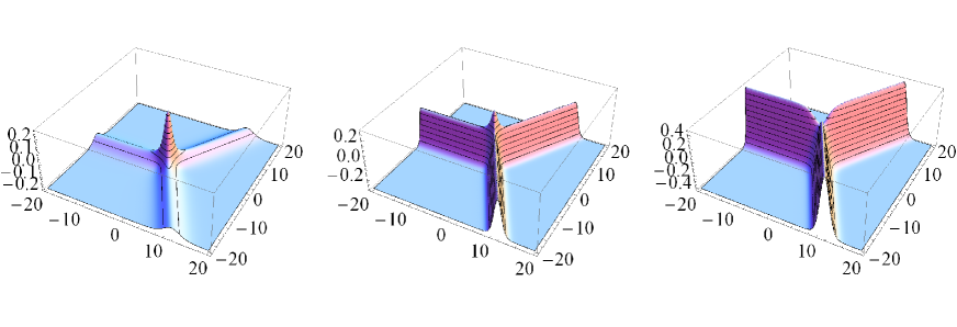
Figure 1: Domain wall junctions in the $N=3$ case. The energy densities are plotted for different choices of the parameters: (1) $\tau\simeq 0.1$ ($\lambda_{1}=\lambda_{2}=1$ and $C/\mu=1/5$), (2) $\tau\simeq 0.5$ ($\lambda_{1}=\lambda_{2}=1$ and $C/\mu=1$), (3) $\tau\simeq 12$ ($\lambda_{1}=\lambda_{2}=1/5$ and $C/\mu=10$). The spatial axes are in units of $m_{1}^{-1}$, and the vertical axis is in units of $Nv^{2}m_{1}^{2}$.

Note that we should anticipate that the Abelian axial vortex might be broken up into three non-Abelian axial vortices. However, the domain wall junctions cannot be broken up as long as we work in the reduced model given in Eq. (41) since no non-Abelian vortices can be described by the reduced equation of motion (41). In order to see if static domain wall junctions exist or not, we should leave more degrees of freedom

$$\Sigma={\rm diag}\left(\phi_{1}(x,y,t),\cdots,\phi_{N}(x,y,t)\right),$$ (42)

where the $N$ complex scalar fields are dealt with as independent fields. In the case where no domain walls exist for $C=0$, well separated non-Abelian axial vortices experience no force at leading order Nakano:2007dq and a repulsive force at the next leading order Eto:2011wp ; Eto:2013hoa , so that the Abelian axial vortex is not likely to be stable as in Eq. (36). Therefore, one would naively expect that there are no static domain wall junctions because the Abelian axial vortex will be easily torn off into $N$ non-Abelian axial vortices since the non-Abelian vortices are pulled by the domain walls toward different directions. Nevertheless, we found static domain wall junctions in the less-reduced models with multiple complex scalar fields in Eq. (42). Several numerical solutions of static domain wall junctions are shown in Fig. 1 for $N=3$ case.

Although we have found static solutions numerically, this does not immediately imply their stability. In our case, they might be just stationary points of the action. Indeed, in the following sections, we will study disintegration of Abelian axial vortices into non-Abelian axial vortices.

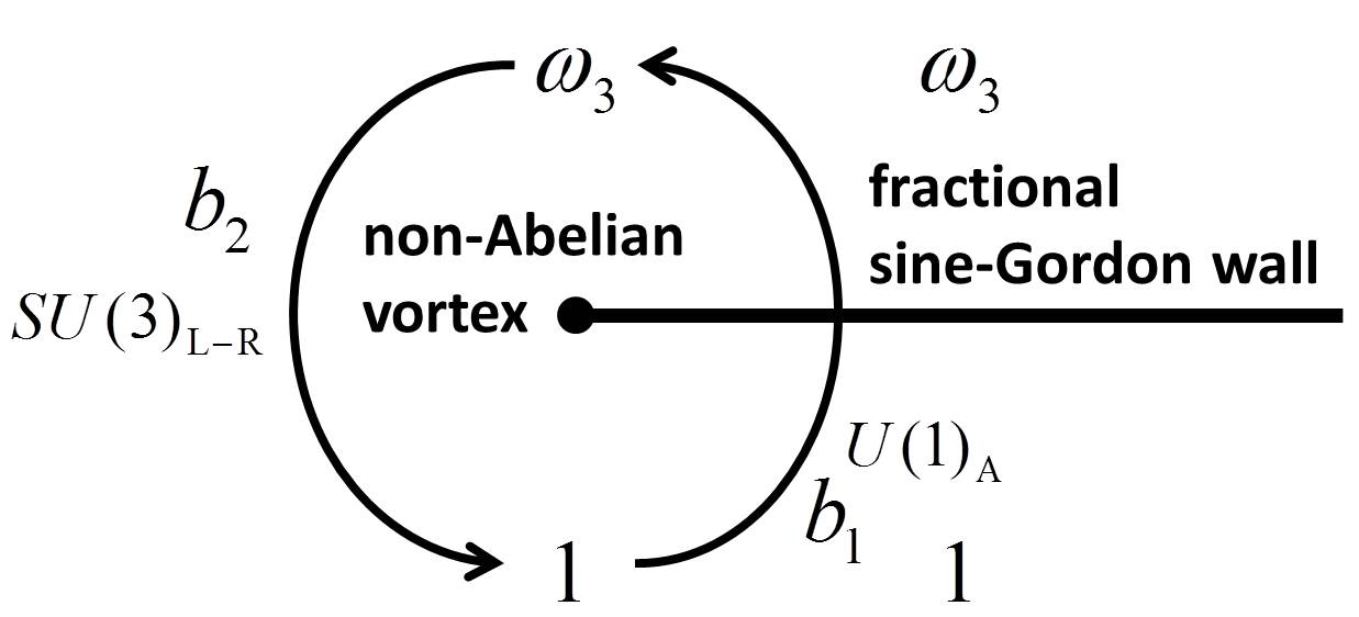
(a)

(b)

Figure 2: (a) Non-Abelian axial vortex attached by a fractional axial domain wall. Along the path $b_{1}$, only the $U(1)_{\rm A}$ phase is rotated by $2\pi/3$. Then, the $SU(3)_{\rm L-R}$ transformation $\exp[(i/3)(\theta-\pi/2)\operatorname{diag}(2,-1,-1)]$ is performed along the path $b_{2}$, where $\theta$ ($\pi/2\leq\theta\leq 3\pi/2$) is the angle of the polar coordinates at the black point. (b) An M₂ non-Abelian axial vortex attached by two fractional axial domain walls.

Let us next consider non-Abelian axial vortices. Since the $U(1)_{\rm A}$ phase changes by $2\pi/N$ around a vortex, one fractional axial wall attaches to one non-Abelian axial vortex as illustrated in Fig. 2(a). Let us examine the structure in more detail, focusing on the configuration of the type $\operatorname{diag}(e^{i\theta},1,\cdots,1)$. In the vicinity of the vortex, let us divide a closed loop encircling the vortex into paths $b_{1}$ and $b_{2}$ as in Fig. 2(a). Then, along paths $b_{1}$ and $b_{2}$, the order parameter receives the transformation by the following group elements:

$$b_{1} : \exp\left[{2i\over N}\left(\theta+{\pi\over 2}\right)\operatorname{diag}(1,1,\cdots,1)\right]\in U(1)_{\rm A},\quad\quad-{\pi\over 2}\leq\theta\leq{\pi\over 2},$$

$$b_{2} : \omega_{N}\exp\left[{2i\over N}\left(\theta-{\pi\over 2}\right)\operatorname{diag}(N-1,-1,\cdots,-1)\right]\in SU(N)_{\rm L-R},\quad{\pi\over 2}\leq\theta\leq{3\over 2}\pi.$$ (43)

Only the $U(1)_{\rm A}$ phase is rotated along path $b_{1}$, while only the $SU(N)_{\rm L-R}$ transformation is performed along path $b_{2}$. This configuration was discussed in Ref. Balachandran:2002je . A numerical solution of the non-Abelian axial vortex with a fractional domain wall is shown in Fig. 3. However, note that the vortex is pulled by the tension of the domain wall and consequently this configuration is not static .

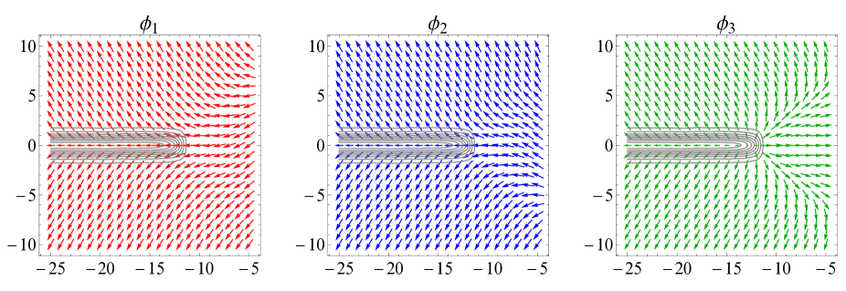
Figure 3: The non-Abelian axial vortex attached by a fractional domain wall for $N=3$. The parameter is $\tau\simeq 0.5$ ($\lambda_{1}=\lambda_{2}=1$ and $C/\mu=1$). The non-Abelian axial vortex $(\phi_{3})$ is located at $(x,y)\sim(-13,0)$ and the domain wall extends toward the $-x$ direction from the vortex. The directions and the magnitudes of the arrows denote the phases of the amplitudes of $\phi_{i}$. The spatial axes are in the unit of $m_{1}^{-1}$.

From Fig. 3, one can see that the domain wall interpolates $\varphi_{\rm A}=2\pi/3$ and $\varphi_{\rm A}=4\pi/3$ which ends on the non-Abelian axial vortex of $\phi_{3}$.

For $N=3$, there is another kind of junctions, called an M₂ non-Abelian vortex Balachandran:2005ev ; Eto:2013hoa . It takes the form

$$\Sigma\xrightarrow[]{r\to\infty}v\,{\rm diag}\left(1,e^{i\theta},e^{i\theta}\right)=v\,e^{i\frac{2\theta}{3}}{\rm diag}\left(e^{-i\frac{2\theta}{3}},e^{i\frac{\theta}{3}},e^{i\frac{\theta}{3}}\right),$$ (44)

in the absence of the instanton-induced potential. In the presence of the instanton-induced potential, the $U(1)_{\rm A}$ phase rotates by $-2\pi/3$. Therefore, two axial domain walls are attached as illustrated in Fig. 2(b) Balachandran:2002je .

V Instability of domain wall junctions

The domain wall junctions shown in Fig. 1 or in Fig. 2(b) were considered to be stable Balachandran:2002je . However, from now on we will show that they are in fact unstable. Here we will study the $N=3$ model for simplicity, but it is straightforward to extend it to generic $N$. A junction of three fractional axial domain walls decays into a set of three fractional axial domain walls, each of which is edged by non-Abelian axial vortices. An Abelian axial vortex is attached by no domain walls in the absence of the instanton-induced potential, as discussed in Sect. III.2. Nevertheless, it can be separated into three non-Abelian axial vortices as in Eq. (36) without binding force at the leading order Nakano:2007dq . Since the axial anomaly is always present in reality, the configuration of a single Abelian axial vortex attached by three domain walls is unstable and it decays as shown in Fig. 4, since each non-Abelian axial vortex is pulled by the tension of a fractional axial domain wall. The $U(1)_{\rm A}$ phase changes by $2\pi/3$ around each non-Abelian axial vortices attached by fractional axial domain walls.

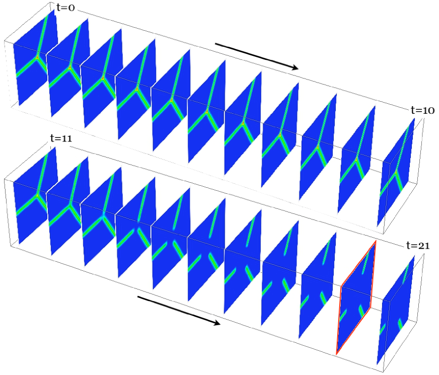
Figure 4: A decay sequence of a three-pronged fractional axial domain wall junction for $N=3$ case. The potential energy densities are plotted. We put tiny random noise around a junction point at $t=0$, which disunites the Abelian axial vortex. The snapshots are taken from $t=0$ to $t=21$ with $\Delta t=1$. The parameter is $\tau\simeq 0.5$ ($\lambda_{1}=\lambda_{2}=1$ and $C/\mu=1$). The plotted region is $x\in(-20,20)$, $y\in(-20,20)$ in units of $m_{1}^{-1}$. We have taken the configuration in Fig. 3 from the panel outlined with a red square at $t=20$. The colors correspond to the height of the potential energy density as blue (low energy) $\to$ green $\to$ yellow $\to$ red (high energy).

We show the detailed configuration of a decaying junction in Fig. 5. The Abelian axial vortex initially located at the origin O decays into three non-Abelian axial vortices, denoted by the red, green, and blue dots. The three fractional axial domain walls denoted by the red, blue, and green dotted lines initially separate $\Sigma\sim{\bf 1}_{3}$ and $\omega_{3}{\bf 1}_{3}$, $\omega_{3}{\bf 1}_{3}$ and $\omega_{3}^{-1}{\bf 1}_{3}$, and $\omega_{3}^{-1}{\bf 1}_{3}$ and ${\bf 1}_{3}$, respectively. The red, blue, and green non-Abelian axial vortices are encircled by the paths $b_{1}-r_{3}+r_{2},b_{2}-r_{1}+r_{3},b_{3}-r_{2}+r_{1}$ respectively. At the boundary of the spatial infinity, the $U(1)_{\rm A}$ phase is rotated by $\exp[i\theta\operatorname{diag}(1,1,1)]$ with the angle $\theta$ of the polar coordinates from the origin O. Therefore, the $U(1)_{\rm A}$ phase is rotated by $2\pi/3$ along each of the paths $b_{1}$, $b_{2}$ and $b_{3}$. Let us suppose that the three paths enclose the three configurations in Eq. (33), respectively. Then, we find that the transformations $g(r)\in SU(3)_{\rm L-R}$ occur along the paths $r_{1}$, $r_{2}$ and $r_{3}$ as

$$r_{1}: g(r)=\exp[iu(r)\operatorname{diag}(0,-1,1)]=\bigg{\{}\begin{array}[]{c}\operatorname{diag}(1,1,1),\quad r=0\cr\operatorname{diag}(1,\omega_{3}^{-1},\omega_{3}),\quad r=\infty\end{array},$$ (47)

$$r_{2}: g(r)=\exp[iu(r)\operatorname{diag}(1,0,-1)]=\bigg{\{}\begin{array}[]{c}\operatorname{diag}(1,1,1),\quad r=0\cr\operatorname{diag}(\omega_{3},1,\omega_{3}^{-1}),\quad r=\infty\end{array},$$ (50)

$$r_{3}: g(r)=\exp[iu(r)\operatorname{diag}(-1,1,0)]=\bigg{\{}\begin{array}[]{c}\operatorname{diag}(1,1,1),\quad r=0\cr\operatorname{diag}(\omega_{3}^{-1},\omega_{3},1),\quad r=\infty\end{array},$$ (53)

respectively, where $u(r)$ is a monotonically increasing function with the boundary conditions $u(r=0)=0$ and $u(r=\infty)=2\pi/3$. We find that the origin O is consistently given by $\Sigma=v\operatorname{diag}(\omega_{3}^{-1},1,\omega_{3})$. From a symmetry, permutations of each component are equally possible. An M₂ non-Abelian axial vortex in Fig. 2(b) also decays into two non-Abelian axial vortices for the same reason.

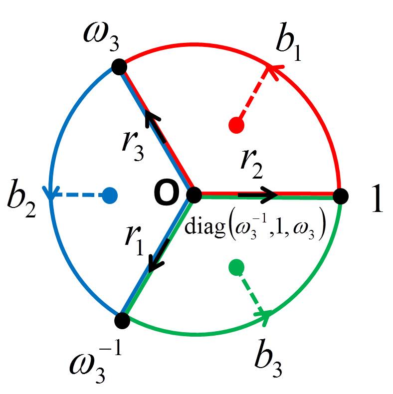
Figure 5: Classical decay of an axial domain wall junction. See text for explanation.

The configurations studied here are topologically the same Eto:2013hoa with a $U(1)_{\rm B}$ superfluid vortex broken into a set of three semi-superfluid non-Abelian vortices in dense QCD Balachandran:2005ev ; Eto:2009kg ; Eto:2009bh .

Note that there is a sharp contrast to the axion strings. Though an axion string in the $N=3$ axion model also gets attached by three domain walls, the domain walls cannot tear off the axion string into three fractional strings Vilenkin:1994 .

Before closing this section, let us make a comment on the effects by quark masses. The quark masses can be taken into account in the effective Lagrangian (9), as an additional term ${\rm Tr}\left[M(\Sigma+\Sigma^{\dagger})\right]$ with $M\propto{\rm diag}(m_{u},m_{d},m_{s})$. In order to see the deformation of the potential, it is useful to use the restricted field given in Eq. (15) again, and one finds that the axial phase receives an additional potential $\sim v(m_{u}+m_{d}+m_{s})\cos\varphi_{\rm A}$. So the potential has two terms $\cos 3\varphi_{\rm A}$ and $\cos\varphi_{\rm A}$ in competition with each other. When the quark masses are small enough to be neglected, the Abelian axial vortex is torn off by three domain walls. On the other hand, when the quark masses are large enough compared to the instanton-induced potential, there is only one true ground state, so that the Abelian axial vortex cannot be separated into three non-Abelian axial strings. The three domain walls are glued into one fat domain wall and it will attach to an Abelian axial vortex. A detailed analysis, including numerical solutions, is given elsewhere Eto:2013hoa .

VI Quantum decay of axial domain walls

We here discuss the quantum decay of fractional axial domain walls. Although this domain wall is classically stable, it turns out to be metastable if one takes into account the quantum tunneling effect. Inside a fractional axial domain wall, quantum (or thermal) fluctuations make holes, which are edged with non-Abelian vortices. If a hole exceeds the critical size, it expands, just as a leaf is eaten by caterpillars, because of the tension of the domain wall. Eventually, the domain wall disappears Bachas:1994ds . The energy of the domain walls mainly turns into to the radiated $\eta^{\prime}$ mesons and pions.

This should be contrasted with the $N>1$ axion model, where the potential has the same periodicity $\varphi_{\rm A}\sim\varphi_{\rm A}+2\pi/N$ and domain walls are stable. The difference comes from the fact that degenerate ground states in the case of chiral phase transition can be connected by a path in the $SU(N)_{\rm L-R}$ group without a potential, as explained above. Let us first consider $d=2+1$ dimensions for simplicity. Suppose we have an axial domain wall interpolating between $\Sigma\sim{\bf 1}_{N}$ and $\Sigma\sim\omega_{N}{\bf 1}_{N}$ as in the left panel of Fig. 6. This wall can decay by creating path $c$ in the right panel of Fig. 6, along which the two ground states $1$ and $\omega_{N}$ are connected by

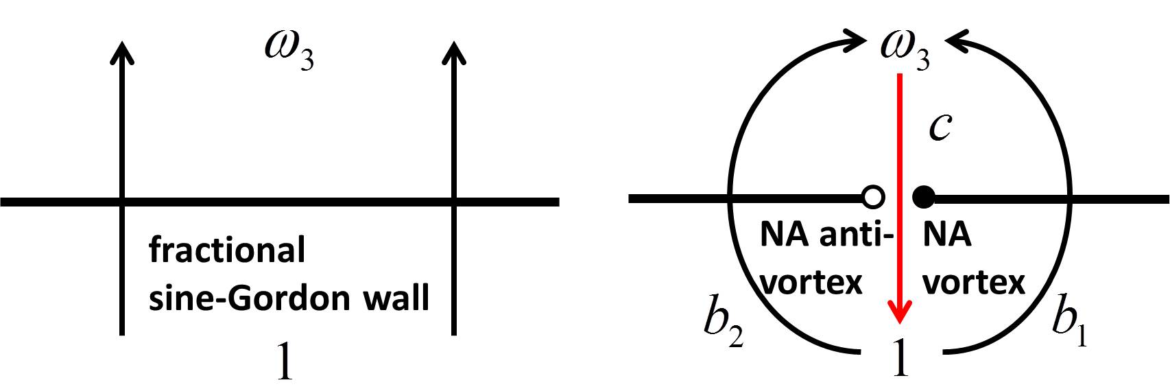
Figure 6: Quantum decay of a fractional axial domain wall. A pair of a non-Abelian axial vortex and a non-Abelian axial anti-vortex is created.

$$\omega_{N}\,\exp\left[{i\over N}\left(\theta-{\pi\over 2}\right)\operatorname{diag}(N-1,-1,\cdots,-1)\right]=\bigg{\{}\begin{array}[]{c}\omega_{N},\quad\theta={\pi\over 2}\cr 1,\quad\theta={3\over 2}\pi\end{array}$$ (56)

in the $SU(N)_{\rm L-R}$ group ($\pi/2\leq\theta\leq 3\pi/2$). Here $\theta$ represents the angle from the black point. Then, one finds that the counterclockwise loop $b_{1}+c$ encloses a non-Abelian axial vortex of the type diag$(e^{i\theta},1,\cdots,1)$ (represented by the black point). This is nothing but the configuration in Fig. 2. The clockwise closed loop $-b_{2}+c$ also encloses a non-Abelian axial vortex (denoted by a white point), which implies that it is an non-Abelian axial anti-vortex. Therefore, a hole bounded by a pair of a non-Abelian axial vortex and a non-Abelian axial anti-vortex is created. When one deforms the path $b_{1}$ to $-c$ in Fig. 6, one must create a non-Abelian vortex, implying an energy barrier between these two paths. Therefore, the domain wall is metastable.

In $d=3+1$ dimensions, a 2D hole bounded by a closed non-Abelian axial vortex loop is created. Through this decay process, the domain wall energy turns into radiation of the $U(N)_{\rm L-R+A}$ Nambu-Goldstone modes ($\eta^{\prime}$ mesons and pions).

The decay rate of axial domain walls can be calculated as follows Preskill:1992ck . Once a hole is created on the integer axial wall, it will expand if the size of this hole is larger than a critical value, and the axial domain wall decays. We calculate the quantum tunneling probability of this process. Let $R$ be the initial radius of a hole created on the axial domain wall. Then, the bounce action of this tunneling process is

$$B=4\pi R^{2}T_{\rm v}-\frac{4}{3}\pi R^{3}T_{\rm w},$$ (57)

where $T_{U(N)_{\rm L-R+A}}$ and $T_{\rm w}$ are the tensions of the vortex and the axial domain wall, given in Eqs. (34) and (19), respectively. The critical radius $R_{\rm c}$ is the one that minimizes this bounce action, given by $R_{\rm c}=2T_{U(N)_{\rm L-R+A}}/T_{\rm w}.$ Thus, the decay rate is

$$P \sim e^{-B}\big{|}_{R=R_{\rm c}}=\exp\left(-\frac{16\pi}{3}\frac{T_{U(N)_{\rm L-R+A}}^{3}}{T_{\rm w}^{2}}\right)$$ (58)

$$= \exp\left(-\frac{N^{2}\pi^{4}v^{2}}{6m_{\eta^{\prime}}^{2}}\left(\log\frac{L}{\xi_{\rm na}}\right)^{3}\right).$$ (59)

VII Summary and Discussion

We have studied domain walls and vortices in the broken phase of the chiral symmetry in QCD with $N$ flavors in the chiral limit. In the absence of the axial anomaly, there exist stable Abelian axial vortices winding around the spontaneously broken $U(1)_{\rm A}$ symmetry and non-Abelian axial vortices winding around both the $U(1)_{\rm A}$ and non-Abelian $SU(N)$ chiral symmetries. In the presence of the axial anomaly term, metastable domain walls are present and vortices cannot exist alone. Abelian axial vortices are attached by $N$ domain walls forming domain wall junctions, and a non-Abelian axial vortex is attached by a domain wall. We have argued that a domain wall junction can topologically decay into $N$ non-Abelian vortices attached by domain walls implying its metastability, and simulated such a decay numerically. We have also shown that domain walls can decay quantum-mechanically by creating a hole bounded by a closed non-Abelian vortex.

In order to study whether the domain wall problem exists, we have to estimate how many domain walls are created in the phase transition by the Kibble-Zurek mechanism Kibble:1976sj ; Hindmarsh:1994re ; Zurek:1985qw ; Zurek:1996sj . Since the chiral symmetry breaking is actually a crossover rather than a phase transition, the estimation of the domain wall number density is not straightforward. Then, the mechanism found in this paper would reduce the number of domain walls. Numerical simulation of the production and decay of domain walls remains as an important future problem. It would also be interesting to study these processes in heavy-ion collisions.

As described in the introduction, the same discussions in this paper hold for chiral symmetry breaking in high-density QCD Eto:2013hoa . However, there is also a difference because of the color degrees of freedom in the symmetry breaking; In addition to the non-Abelian axial vortices discussed in this paper, there are also non-Abelian semi-superfluid vortices, which are color magnetic flux tubes Balachandran:2005ev ; Nakano:2007dr ; Nakano:2008dc ; Eto:2009kg ; Eto:2009bh ; Eto:2009tr ; Hirono:2010gq . The roles played by these flux tubes is an open question.

References

- (1) R.D. Peccei and Helen R. Quinn, Phys.Rev.Lett., 38, 1440–1443 (1977).
- (2) R.D. Peccei and Helen R. Quinn, Phys.Rev., D16, 1791–1797 (1977).
- (3) Steven Weinberg, Phys.Rev.Lett., 40, 223–226 (1978).
- (4) Frank Wilczek, Phys.Rev.Lett., 40, 279–282 (1978).
- (5) P. Sikivie, Phys.Rev.Lett., 48, 1156–1159 (1982).
- (6) Michael Dine, Willy Fischler, and Mark Srednicki, Phys.Lett., B104, 199 (1981).
- (7) Michael McNeil Forbes and Ariel R. Zhitnitsky, JHEP, 0110, 013 (2001).
- (8) Xinmin Zhang, Tao Huang, and Robert H. Brandenberger, Phys.Rev., D58, 027702 (1998).
- (9) A.P. Balachandran and S. Digal, Int.J.Mod.Phys., A17, 1149–1158 (2002).
- (10) A.P. Balachandran and S. Digal, Phys.Rev., D66, 034018 (2002).
- (11) Muneto Nitta and Noriko Shiiki, Phys.Lett., B658, 143–147 (2008).
- (12) Eiji Nakano, Muneto Nitta, and Taeko Matsuura, Phys.Lett., B672, 61–64 (2009).
- (13) Minoru Eto, Eiji Nakano, and Muneto Nitta, Nucl.Phys., B821, 129–150 (2009).
- (14) Minoru Eto, Yuji Hirono, Muneto Nitta, and Shigehiro Yasui, PTEP, 2014(1), 012D01 (2013).
- (15) Mark G. Alford, Krishna Rajagopal, and Frank Wilczek, Phys.Lett., B422, 247–256 (1998).
- (16) Mark G. Alford, Krishna Rajagopal, and Frank Wilczek, Nucl.Phys., B537, 443–458 (1999).
- (17) Mark G. Alford, Andreas Schmitt, Krishna Rajagopal, and Thomas Schafer, Rev.Mod.Phys., 80, 1455–1515 (2008).
- (18) R. Casalbuoni and Raoul Gatto, Phys.Lett., B464, 111–116 (1999).
- (19) Robert D. Pisarski and Frank Wilczek, Phys.Rev., D29, 338–341 (1984).
- (20) T.H.R. Skyrme, Proc.Roy.Soc.Lond., A262, 237–245 (1961).
- (21) J.K. Perring and T.H.R. Skyrme, Nucl.Phys., 31, 550–555 (1962).
- (22) D.T. Son and M.A. Stephanov, Phys.Rev., D77, 014021 (2008).
- (23) A.P. Balachandran, S. Digal, and T. Matsuura, Phys.Rev., D73, 074009 (2006).
- (24) Minoru Eto, Kenichi Kasamatsu, Muneto Nitta, Hiromitsu Takeuchi, and Makoto Tsubota, Phys.Rev., A83, 063603 (2011).
- (25) Minoru Eto and Muneto Nitta, Phys.Rev., D80, 125007 (2009).
- (26) Minoru Eto, Eiji Nakano, and Muneto Nitta, Phys.Rev., D80, 125011 (2009).
- (27) Alexander Vilenkin and E Paul S Shellard, Cosmic strings and other topological defects, (Cambridge University Press, 2000).
- (28) C. Bachas and T.N. Tomaras, Nucl.Phys., B428, 209–220 (1994).
- (29) John Preskill and Alexander Vilenkin, Phys. Rev., D47, 2324–2342 (1993).
- (30) T.W.B. Kibble, J.Phys., A9, 1387–1398 (1976).
- (31) M.B. Hindmarsh and T.W.B. Kibble, Rept.Prog.Phys., 58, 477–562 (1995).
- (32) W.H. Zurek, Nature, 317, 505–508 (1985).
- (33) W.H. Zurek, Phys.Rept., 276, 177–221 (1996).
- (34) Eiji Nakano, Muneto Nitta, and Taeko Matsuura, Phys.Rev., D78, 045002 (2008).
- (35) Eiji Nakano, Muneto Nitta, and Taeko Matsuura, Prog.Theor.Phys.Suppl., 174, 254–257 (2008).
- (36) Minoru Eto, Muneto Nitta, and Naoki Yamamoto, Phys.Rev.Lett., 104, 161601 (2010).
- (37) Yuji Hirono, Takuya Kanazawa, and Muneto Nitta, Phys.Rev., D83, 085018 (2011).