Power Optimization for Network Localization

Abstract

Reliable and accurate localization of mobile objects is essential for many applications in wireless networks. In range-based localization, the position of the object can be inferred using the distance measurements from wireless signals exchanged with active objects or reflected by passive ones. Power allocation for ranging signals is important since it affects not only network lifetime and throughput but also localization accuracy. In this paper, we establish a unifying optimization framework for power allocation in both active and passive localization networks. In particular, we first determine the functional properties of the localization accuracy metric, which enable us to transform the power allocation problems into second-order cone programs. We then propose the robust counterparts of the problems in the presence of parameter uncertainty and develop asymptotically optimal and efficient near-optimal SOCP-based algorithms. Our simulation results validate the efficiency and robustness of the proposed algorithms.

I Introduction

Network localization of active and passive objects is essential for many location-based applications in commercial, military, and social sectors [1, 2, 3, 4, 5, 6, 7, 8]. Contemporary localization techniques can be classified into two main categories, i.e., range-based and range-free techniques. The former locate the object using distance/angle measurements [1, 2, 3, 4], and the latter using connectivity or fingerprint information [9, 10, 11, 12]. Compared to range-free ones, range-based techniques are more suited and hence widely employed for high-accuracy localization despite the hardware complexity. Active or passive localization refers to the rang-based techniques that utilize distance/angle measurements from wireless signals exchanged with active objects or reflected by passive ones, respectively. Two corresponding examples are wireless network localization (WNL) [1, 2, 3, 4] and radar network localization (RNL) [7, 5, 6, 8] (see Fig. 1).

Wireless networks have been employed for active localization since they are capable of providing accurate position information in GPS-challenged environments [2, 1, 4, 3, 13, 14, 15, 16, 17, 18]. Locating a mobile node (agent) in such networks can be accomplished by using the range measurements between the agent and nodes at known positions (anchors). The ranges can be estimated from the time-of-arrival (TOA) or received signal strength (RSS) of the signals transmitted from the anchors to the agent [19, 20, 21, 22, 23, 24]. Localization accuracy in wireless networks is determined by the network topology and the accuracy of the range measurements, where the latter depends on the signal bandwidth, channel condition, and transmit power [19]. Hence, power allocation in WNL is important not only for the conventionally recognized lifetime and throughput [25] but also for agent localization accuracy.

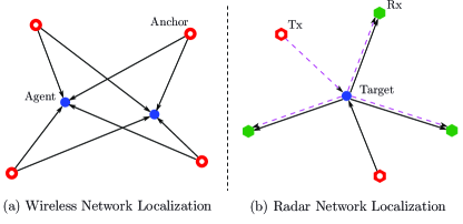
Figure 1: Network deployments for WNL and RNL: (a) wireless network with four anchors and two agents; (b) radar network with two transmit and three receive antennas.

Radar networks have been studied for passive localization since they can enhance target detection and localization capability by exploiting the spatial diversity of target’s radar cross section (RCS) [26, 6, 27, 7, 28, 29, 30, 5, 31]. The target can be located using the TOA range measurements from the transmit to receive antennas via the reflection of the target. Localization accuracy in radar networks depends on the network topology, signal bandwidth, target RCS, and transmit power [6]. Hence, power allocation and management in RNL is crucial not only for low-probability-of-intercept (LPI) capability [32] but also for target localization accuracy.

The main task of power allocation for network localization is to achieve the optimal tradeoffs between localization accuracy and energy consumption. Such a task is commonly accomplished using optimization methods, which have played a significant role in maximizing communication and networking performance under limited resources [33, 34, 35, 36, 37, 38, 39]. One can formulate the power allocation problem for network localization by constraining either the localization error or total transmit power and minimizing the other. Solving these problems requires the knowledge of network parameters, which in practice are subject to uncertainty. Ignoring such uncertainty will lead to sub-optimal or even infeasible solutions [39, 40, 41, 42]. Hence, two fundamental questions related to power allocation in network localization are:

1. how to minimize the total transmit power while satisfying the localization requirement;

2. how to guarantee the localization requirement in the presence of parameter uncertainty.

Answers to these questions will provide insights into the essence of network localization and enable the design of robust network algorithms.

Several formulations have been proposed for power allocation in different localization scenarios using the performance metrics based on the information inequality [43, 44, 6, 45]. For WNL, the optimal power allocation solution was determined in closed forms for specific network topologies [43] and was obtained by an semidefinite program (SDP) for general network topologies [44]. For RNL, a suboptimal power allocation algorithm was developed via a relaxation technique [6]. Most studies assume perfect knowledge of the network parameters with the exception of [44], in which a robust formulation was proposed to cope with small parameter uncertainty and a suboptimal solution was obtained through relaxation. However, the performance loss from the relaxation was not quantified since the optimal solution of the robust formulation remains unknown.

In this paper, we investigate the optimal power allocation problem for reliable and accurate network localization, aiming to minimize the total transmit power for a given localization requirement. Our work also encompasses robust counterparts to cope with the parameter uncertainty. The main contributions of this paper are as follows.

• We establish a unifying optimization framework for power allocation in both active and passive localization networks through WNL and RNL examples.

• We determine the functional properties of the localization accuracy metric and transform the power allocation problems into SOCPs.

• We propose a robust power allocation formulation that guarantees the localization requirement in the presence of parameter uncertainty over large ranges.

• We develop asymptotically optimal and efficient near-optimal SOCP-based algorithms for the robust formulation, and characterize the convergence rate of the asymptotic algorithms to the optimal solution.

The rest of the paper is organized as follows. In Section II, we introduce the system models and formulate the power allocation problems. In Section III, we present the properties of the localization accuracy metric and show that the power allocation problems can be transformed into SOCPs. In Section IV, we present robust formulations for the case with parameter uncertainty and develop asymptotically optimal and efficient near-optimal algorithms. In Section V, we give some comments and discussions on the results. Finally, the performance of the proposed algorithms is evaluated by simulations in Section VI, and conclusions are drawn in the last section.

Notation: $\mathbb{S}_{+}^{n}$ denotes the set of $n\times n$ positive-semidefinite matrices; matrices $\mathbf{A}\succeq\mathbf{B}$ denotes that $\mathbf{A}-\mathbf{B}$ is positive semidefinite; vectors $\mathbf{x}\succeq\mathbf{y}$ denotes that all elements of $\mathbf{x}-\mathbf{y}$ are nonnegative; $\mathbf{1}_{n}\in\mathbb{R}^{n}$ denotes a column vector with all 1’s, $\mathbf{0}_{n}\in\mathbb{R}^{n}$ denotes a column vector with all 0’s, and $\mathbf{I}_{n}\in\mathbb{R}^{n\times n}$ denotes an identity matrix, where the subscript $n$ will be omitted if clear in the context; vector $\mathbf{u}(\phi):=[\,\cos\phi~{}\sin\phi\,]^{\text{T}}$; matrix $\mathbf{J}_{\text{r}}(\phi):=\mathbf{u}(\phi)\,\mathbf{u}(\phi)^{\text{T}}$; and we define the functions

$$\mathbf{c}(\boldsymbol{\phi}) :=[\,\cos\phi_{1}\;\;\cos\phi_{2}\;\;\cdots\;\;\cos\phi_{n}\,]^{\text{T}}$$

$$\mathbf{s}(\boldsymbol{\phi}) :=[\,\sin\phi_{1}\;\;\sin\phi_{2}\;\;\cdots\;\;\sin\phi_{n}\,]^{\text{T}}$$

where $\boldsymbol{\phi}=[\,\phi_{1}~{}~{}\phi_{2}~{}~{}\cdots~{}~{}\phi_{n}\,]^{\text{T}}$.

II Problem Formulation

In this section, we introduce the system models, present the performance metric, and formulate the power allocation problems for WNL and RNL.

II-A System Models

We first introduce the system models for WNL and RNL.

Wireless Network Localization

Consider 2-D wireless localization using a location-aware network with ${{N}_{\text{b}}}$ anchors and ${N_{\text{a}}}$ agents [see Fig. 1(a)]. The sets of anchors and agents are denoted by ${\mathcal{N}_{\text{b}}}$ and ${\mathcal{N}_{\text{a}}}$, respectively. The position of node $k$ is denoted by $\mathbf{p}_{k}\in\mathbb{R}^{2}$ for $k\in{\mathcal{N}_{\text{b}}}\cup{\mathcal{N}_{\text{a}}}$, and the angle and distance from nodes $k$ to $j$ are denoted by $\phi_{kj}$ and $d_{kj}$, respectively. The anchors are the nodes with known positions, whereas the agents are mobile nodes aiming to infer their positions based on the TOA range measurements from the anchors [19].

The equivalent lowpass waveform received at agent $k$ from anchor $j$ is modeled as [19]

$$r_{k}(t)=\sum_{j\in{\mathcal{N}_{\text{b}}}}\frac{\sqrt{x_{j}}}{d_{kj}^{\,\beta}}\,\alpha_{kj}\,s_{j}(t-\tau_{kj})+z_{kj}(t)$$ (1)

where $x_{j}$ is the transmit power of anchor $j$ measured at 1 m away from the transmitter, $\beta$ is the amplitude loss exponent, $\{s_{j}(t)\}_{j\in{\mathcal{N}_{\text{b}}}}$ is a set of the orthonormal transmit waveforms, $\alpha_{kj}$ and $\tau_{kj}$ are the amplitude gain and propagation delay, respectively, and $z_{kj}(t)$ represents the observation noise, modeled as additive white complex Gaussian processes. The relationship between the delay and agent’s position is

$$\tau_{kj}=\frac{1}{c}\,\|\mathbf{p}_{k}-\mathbf{p}_{j}\|$$

where $c$ is the propagation speed of the signal.

The agents’ positions $\{\mathbf{p}_{k}\}_{k\in{\mathcal{N}_{\text{a}}}}$ are inferred using the measurements $\{r_{k}(t)\}_{k\in{\mathcal{N}_{\text{a}}}}$. Since the channel parameters are also unknown, the complete set of unknown deterministic parameters is given by $\boldsymbol{\theta}=\{\mathbf{p}_{k},\,\alpha_{kj}\}_{k\in{\mathcal{N}_{\text{a}}},\,j\in{\mathcal{N}_{\text{b}}}}$.

Radar Network Localization

Consider 2-D target localization using a radar network with ${N_{\text{t}}}$ transmit and ${{N}_{\text{r}}}$ receive antennas [see Fig. 1(b)]. The sets of transmit and receiver antennas are denoted by ${\mathcal{N}_{\text{t}}}$ and ${\mathcal{N}_{\text{r}}}$, respectively. The position of antenna $k$ is known and denoted by $\mathbf{p}_{k}\in\mathbb{R}^{2}$ for $k\in{\mathcal{N}_{\text{t}}}\cup{\mathcal{N}_{\text{r}}}$, and the position of the target is denoted by $\mathbf{p}_{0}\in\mathbb{R}^{2}$. The angle from antenna $k$ to the target is given by $\psi_{k}$ for $k\in{\mathcal{N}_{\text{r}}}$ or $\varphi_{k}$ for $k\in{\mathcal{N}_{\text{t}}}$, and the corresponding distance is given by $d_{k}$. The radar network aims to locate the target based on the TOA range measurements from the transmit to receive antennas via the reflection of the target [5].

The equivalent lowpass waveform received at antenna $k$ from the transmit antennas is modeled as[5]

$$r_{k}(t)=\sum_{j\in{\mathcal{N}_{\text{t}}}}\frac{\sqrt{x_{j}}}{d_{k}^{\,\beta}d_{j}^{\,\beta}}\,\alpha_{kj}\,s_{j}\left(t-\tau_{kj}\right)+z_{kj}(t)$$ (2)

where $x_{j}$ is the transmit power of antenna $j$, $\{s_{j}(t)\}_{j\in{\mathcal{N}_{\text{t}}}}$ is a set of the orthonormal transmit waveforms, and $\alpha_{kj}$ and $\tau_{kj}$ are the amplitude gain and propagation delay. Then the relationship between the delay and target’s position is

$$\tau_{kj}=\frac{1}{c}(\|\mathbf{p}_{k}-\mathbf{p}_{0}\|+\|\mathbf{p}_{j}-\mathbf{p}_{0}\|)\,.$$

The target’s position $\mathbf{p}_{0}$ is estimated using the measurements $\{r_{k}(t)\}_{k\in{\mathcal{N}_{\text{r}}}}$ by noncoherent processing. Since channel parameters are also unknown, the complete set of unknown deterministic parameters is given by $\boldsymbol{\theta}=\{\mathbf{p}_{0},\,\alpha_{kj}\}_{k\in{\mathcal{N}_{\text{r}}},\,j\in{\mathcal{N}_{\text{t}}}}$.

II-B Performance Metric

We now present the performance metric for localization accuracy as a function of the power allocation vector (PAV) denoted by

$$\mathbf{x}=[\,x_{1}~{}~{}x_{2}~{}~{}\cdots~{}~{}x_{n}\,]^{\text{T}}$$

where $n={{N}_{\text{b}}}$ for WNL and $n={N_{\text{t}}}$ for RNL. For conciseness, we only present the notions for WNL, as they are applicable to RNL analogously.

Localization accuracy can be quantified by the mean squared error (MSE) of the position estimator. Let $\hat{\mathbf{p}}_{k}$ be an unbiased position estimator for agent $k$ in WNL, then the MSE matrix of $\hat{\mathbf{p}}_{k}$ satisfies

$$\mathbb{E}_{\mathbf{r}}\big{\{}(\hat{\mathbf{p}}_{k}-\mathbf{p}_{k})(\hat{\mathbf{p}}_{k}-\mathbf{p}_{k})^{\text{T}}\big{\}}\succeq\mathbf{J}_{\text{e}}^{-1}(\mathbf{p}_{k};\mathbf{x})$$

where $\mathbf{J}_{\text{e}}(\mathbf{p}_{k};\mathbf{x})$ is the equivalent Fisher information matrix (EFIM) for $\mathbf{p}_{k}$ [19]. Consequently, the MSE of the position estimate $\mathbb{E}_{\mathbf{r}}\big{\{}\|\hat{\mathbf{p}}_{k}-\mathbf{p}_{k}\|^{2}\big{\}}$ is bounded below by the squared position error bound (SPEB), defined as [19]

$$\mathcal{P}(\mathbf{p}_{k};\mathbf{x}):=\text{tr}\big{\{}\mathbf{J}_{\text{e}}^{-1}(\mathbf{p}_{k};\mathbf{x})\big{\}}$$ (3)

and hence we adopt the SPEB as the performance metric for WNL. More discussion on the SPEB is given in Section V-C. We next present the EFIMs for WNL and RNL.

Proposition 1

The EFIM for the position of agent $k$ in WNL based on (1) is given by

$$\mathbf{J}_{\text{e}}(\mathbf{p}_{k};\mathbf{x})=\!\sum_{j\in{\mathcal{N}_{\text{b}}}}x_{j}\,\xi_{kj}\cdot\mathbf{J}_{\text{r}}(\phi_{kj})$$ (4)

where the equivalent ranging coefficient (ERC) $\xi_{kj}={\zeta_{kj}}/{d_{kj}^{\,2\beta}}$, in which the ranging coefficient (RC) $\zeta_{kj}\geq 0$ is determined by the channel parameters, signal bandwidth, and noise power.

Proof:

Refer to [19] for the detailed derivation. ∎

Proposition 2

The EFIM for the position of the target in RNL based on (2) is given by

$$\mathbf{J}_{\text{e}}(\mathbf{p}_{0};\mathbf{x})=\!\sum_{j\in{\mathcal{N}_{\text{t}}}}\sum_{k\in{\mathcal{N}_{\text{r}}}}x_{j}\,\xi_{kj}\cdot\mathbf{J}_{\text{r}}(\phi_{kj})$$ (5)

where $\phi_{kj}={(\psi_{k}+\varphi_{j})}/{2}$ and the ERC

$$\xi_{kj}=\frac{4\,\zeta_{kj}}{d_{k}^{\,2\beta}d_{j}^{\,2\beta}}\cos^{2}\Big{(}\frac{\psi_{k}-\varphi_{j}}{2}\Big{)}$$ (6)

in which the RC $\zeta_{kj}\geq 0$ is determined by the channel parameters, signal bandwidth, and noise power.

Proof:

Similar to the derivation in [6], the EFIM based on (2) can be derived as

$$\mathbf{J}_{\text{e}}(\mathbf{p}_{0};\mathbf{x}) =\sum_{j\in{\mathcal{N}_{\text{t}}}}\frac{x_{j}}{d_{j}^{\,2\beta}}\,\sum_{k\in{\mathcal{N}_{\text{r}}}}\frac{\zeta_{kj}}{d_{k}^{\,2\beta}}\,\cdot\mathbf{u}_{kj}\,\mathbf{u}_{kj}^{\text{T}}$$ (7)

where $\mathbf{u}_{kj}=\mathbf{u}(\psi_{k})+\mathbf{u}(\varphi_{j})$. It can be shown using the property of the trigonometric functions that

$$\mathbf{u}_{kj}=2\cos\Big{(}\frac{\psi_{k}-\varphi_{j}}{2}\Big{)}\cdot\mathbf{u}\Big{(}\frac{\psi_{k}+\varphi_{j}}{2}\Big{)}$$ (8)

and by substituting (8) into (7), we obtain (5). ∎

Remark 1

The propositions show that the EFIMs for WNL and RNL have a canonical form as a weighted sum of rank-one matrices $\mathbf{J}_{\text{r}}(\phi_{kj})$. These matrices in (4) and (5) respectively characterize the network topology of the anchors and agent for WNL and that of the transmit/receive antennas and target for RNL.

Remark 2

Note that specific transmission technology and waveform model are considered in Section II-A to derive the EFIMs. However, the analytical methods and algorithms developed in this paper are applicable to network localization using general transmission technologies and waveform models, which only affect the RCs but not the structure of the EFIMs. For instance, the waveform model (2) for RNL assumes that the background clutters are removed and the Doppler shifts are corrected for simplicity; nevertheless, such a simplification does not affect the structure of the EFIM.

II-C Power Allocation Formulation

We now formulate the power allocation problems for WNL and RNL, aiming to achieve the optimal tradeoffs between localization accuracy and energy consumption. In particular, we minimize the total transmit power subject to a given localization requirement for the agents or the target, shown as follows.

The power allocation problem for WNL can be formulated as

$$\mathscr{P}_{\text{A}}:\;\;\min_{\{\mathbf{x}\}}\quad \mathbf{1}^{\text{T}}\,\mathbf{x}$$

s.t. $$\mathcal{P}(\mathbf{p}_{k};\mathbf{x})\leq\varrho_{k}\,,\;\;\forall\,k\in{\mathcal{N}_{\text{a}}}$$ (9)

$$c_{l}(\mathbf{x})\leq 0\,,\qquad\;\,\;l=1,2,\ldots,L$$

where $\varrho_{k}$ denotes the localization requirement for agent $k$ and $\{c_{l}(\cdot)\}$ denotes linear constraints on the PAV $\mathbf{x}$, e.g., the individual power constraints for anchors $\mathbf{0}\preceq\mathbf{x}\preceq\mathbf{x}_{\text{max}}$.

Similarly, the power allocation problem for RNL can be formulated as

$$\mathscr{P}_{\text{P}}:\;\;\min_{\{\mathbf{x}\}}\quad \mathbf{1}^{\text{T}}\,\mathbf{x}$$

s.t. $$\mathcal{P}(\mathbf{p}_{0};\mathbf{x})\leq\varrho$$ (10)

$$c_{l}(\mathbf{x})\leq 0\,,\qquad\;\;\,l=1,2,\ldots,L$$

where $\varrho$ denotes the localization requirement for the target.

Remark 3

Note that the EFIMs (4) and (5), corresponding to the SPEBs $\mathcal{P}(\mathbf{p}_{k};\mathbf{x})$ and $\mathcal{P}(\mathbf{p}_{0};\mathbf{x})$, have a similar expression as a function of $\mathbf{x}$. This leads to a similar structure between the localization requirement constraints (9) and (10), and hence $\mathscr{P}_{\text{A}}$ and $\mathscr{P}_{\text{P}}$. Therefore, we can develop optimal power allocation algorithms for the two scenarios under a unifying framework.

III SPEB Properties and SOCP Formulation

In this section, we first explore the properties of the SPEB, and then show that the power allocation problems can be transformed into SOCPs.

III-A SPEB Properties

The following lemma describes the convexity property of the SPEB given in (3) as a function of the PAV and the low rank property of the topology matrix.

Lemma 1

The SPEB of the agent or the target is a convex function of $\mathbf{x}\succeq\mathbf{0}$. Moreover, the SPEB of agent $k$ for WNL can be written as

$$\mathcal{P}(\mathbf{p}_{k};\mathbf{x}) =\frac{4\cdot\mathbf{1}^{\text{T}}\,\mathbf{R}_{k}\,\mathbf{x}}{\mathbf{x}^{\text{T}}\,\mathbf{R}_{k}^{\text{T}}\,\boldsymbol{\Lambda}_{k}\,\mathbf{R}_{k}\,\mathbf{x}}$$ (11)

where the ERC matrix $\mathbf{R}_{k}=\text{diag}\{\xi_{k1},\xi_{k2},\ldots,\xi_{k{{N}_{\text{b}}}}\}$ and the topology matrix $\boldsymbol{\Lambda}_{k}$ is a symmetric matrix of $\text{rank}\{\boldsymbol{\Lambda}_{k}\}\leq 3$, given by

$$\boldsymbol{\Lambda}_{k} =\mathbf{1}\,\mathbf{1}^{\text{T}}-\mathbf{c}(2\boldsymbol{\phi}_{k})\,\mathbf{c}(2\boldsymbol{\phi}_{k})^{\text{T}}-\mathbf{s}(2\boldsymbol{\phi}_{k})\,\mathbf{s}(2\boldsymbol{\phi}_{k})^{\text{T}}$$ (12)

in which $\boldsymbol{\phi}_{k}=[\,\phi_{k1}\;\;\phi_{k2}\;\;\cdots\;\;\phi_{k{{N}_{\text{b}}}}\,]^{\text{T}}$; the SPEB of the target for RNL can be written as

$$\mathcal{P}(\mathbf{p}_{0};\mathbf{x}) =\frac{4\cdot\mathbf{1}^{\text{T}}\,\mathbf{R}\,\mathbf{x}}{\mathbf{x}^{\text{T}}\,\mathbf{R}^{\text{T}}\boldsymbol{\Lambda}\,\mathbf{R}\,\mathbf{x}}$$

where the ERC matrix $\mathbf{R}=\big{[}\,\mathbf{R}_{1}^{\text{T}}~{}~{}\mathbf{R}_{2}^{\text{T}}~{}~{}\cdots~{}~{}\mathbf{R}_{{{N}_{\text{r}}}}^{\text{T}}\,\big{]}^{\text{T}}$ with $\mathbf{R}_{k}=\text{diag}\{\xi_{k1},\xi_{k2},\ldots,\xi_{k{N_{\text{t}}}}\}$ and the topology matrix $\boldsymbol{\Lambda}$ is a symmetric matrix of $\text{rank}\{\boldsymbol{\Lambda}\}\leq 3$, given by

$$\boldsymbol{\Lambda}=\mathbf{1}\,\mathbf{1}^{\text{T}}-\mathbf{c}({2\boldsymbol{\phi}})\,\mathbf{c}({2\boldsymbol{\phi}})^{\text{T}}-\mathbf{s}({2\boldsymbol{\phi}})\,\mathbf{s}({2\boldsymbol{\phi}})^{\text{T}}$$

in which $\boldsymbol{\phi}=\big{[}\,\boldsymbol{\phi}_{1}^{\text{T}}~{}~{}\boldsymbol{\phi}_{2}^{\text{T}}~{}~{}\cdots~{}~{}\boldsymbol{\phi}_{{{N}_{\text{r}}}}^{\text{T}}\,\big{]}^{\text{T}}$ with $\boldsymbol{\phi}_{k}=[\,\phi_{k1}\;\;\phi_{k2}\;\;\cdots\;\;\phi_{k{N_{\text{t}}}}\,]^{\text{T}}$.

Proof:

See Appendix A. ∎

Remark 4

The lemma first shows that the SPEB is a convex function in $\mathbf{x}$, implying that each localization requirement in (9) and (10) is a convex constraint on $\mathbf{x}$. Thus, the power allocation problems $\mathscr{P}_{\text{A}}$ and $\mathscr{P}_{\text{P}}$ are convex programs. Second, the lemma also shows the low rank (at most three) property of the topology matrix $\boldsymbol{\Lambda}_{k}$ and $\boldsymbol{\Lambda}$. The convexity and low rank properties can be exploited to develop efficient power allocation algorithms.

III-B Optimal Power Allocation

We now show that the constraint (9) can be converted to a second-order cone (SOC) form using the SPEB properties given in Lemma 1. Consequently, the power allocation formulation $\mathscr{P}_{\text{A}}$ is equivalent to an SOCP. For conciseness, we denote $\mathbf{c}_{k}=\mathbf{c}(2\boldsymbol{\phi}_{k})$ and $\mathbf{s}_{k}=\mathbf{s}(2\boldsymbol{\phi}_{k})$ in the following.

Proposition 3

The problem $\mathscr{P}_{\text{A}}$ is equivalent to the SOCP

$$\mathscr{P}_{\text{A}}^{\text{SOCP}}:\;\min_{\{\mathbf{x}\}}\quad \mathbf{1}^{\text{T}}\,\mathbf{x}$$

s.t. $$\big{\|}\mathbf{A}_{k}\,\mathbf{R}_{k}\,{\mathbf{x}}+\mathbf{b}_{k}\big{\|}\leq\mathbf{1}^{\text{T}}\,\mathbf{R}_{k}\,{\mathbf{x}}-2\varrho_{k}^{-1},$$

$$\hskip 113.81102pt\forall\,k\in{\mathcal{N}_{\text{a}}}$$ (13)

$$c_{l}(\mathbf{x})\leq 0\,,\qquad\;\;\,l=1,2,\ldots,L$$

where $\mathbf{A}_{k}=[\,\mathbf{c}_{k}~{}~{}\mathbf{s}_{k}~{}~{}\mathbf{0}\,]^{\text{T}}$ and $\mathbf{b}_{k}=[\,0~{}~{}0~{}~{}2\varrho_{k}^{-1}\,]^{\text{T}}$.

Proof:

Let $\mathbf{y}=\mathbf{R}_{k}\,{\mathbf{x}}$. Using (11) and (12) in Lemma 1, we can rewrite $\mathcal{P}(\mathbf{p}_{k};\mathbf{x})\leq\varrho_{k}$ as

$${4}\varrho_{k}^{-1}\cdot\mathbf{1}^{\text{T}}\,\mathbf{y}\leq{(\mathbf{1}^{\text{T}}\,\mathbf{y})^{2}-(\mathbf{c}_{k}^{\text{T}}\,\mathbf{y})^{2}-(\mathbf{s}_{k}^{\text{T}}\,\mathbf{y})^{2}}\,.$$

By completing the square, we have

$$(\mathbf{c}_{k}^{\text{T}}\,\mathbf{y})^{2}+(\mathbf{s}_{k}^{\text{T}}\,\mathbf{y})^{2}+4\varrho_{k}^{-2}\leq(\mathbf{1}^{\text{T}}\,\mathbf{y})^{2}-4\varrho_{k}^{-1}\cdot\mathbf{1}^{\text{T}}\,\mathbf{y}+4\varrho_{k}^{-2}$$

which is equivalent to (13) since $\mathbf{1}^{\text{T}}\,\mathbf{y}-2\varrho_{k}^{-1}\geq 0$. ∎

Remark 5

This SOCP formulation is more favorable than the SDP formulation proposed in [44], since SOCP is a subclass of SDP and has more efficient solvers than SDP [46]. Moreover, as later shown in Section IV, the SOC form of the localization requirement given in (13) enables better relaxation than the SDP formulation.

Note that a similar SOCP formulation for RNL can be obtained since the problem $\mathscr{P}_{\text{P}}$ has a similar structure as $\mathscr{P}_{\text{A}}$. We omit the details for brevity.

III-C Discussion

The constraints (13) in $\mathscr{P}_{\text{A}}^{\text{SOCP}}$ are determined by the network parameters, including the inter-node angles, distances, and RCs. However, perfect knowledge of these parameters is usually not available; especially, the angles and distances depend on the agents’ positions, which are to be determined. One approach is to use estimated values of the parameters in the power allocation algorithms. Since these estimated values are subject to uncertainty, directly using them in the algorithms often fails to yield reliable or even feasible solutions. Hence, we will next develop robust methods to cope with the parameter uncertainty.

IV Robust Power Allocation Algorithms

In this section, we first introduce the uncertainty models for network parameters and formulate robust power allocation problems. We then develop an asymptotically optimal algorithm with a proven convergence rate and efficient near-optimal algorithms using relaxation methods.

IV-A Uncertainty Models

Based on the robust optimization framework [39, 40, 41], we consider set-based uncertainty models for the network parameters in WNL and RNL.

Wireless Network Localization

Consider the unknown position of agent $k$ in an area $\mathcal{A}_{k}$, and the goal of robust power allocation is to guarantee the localization requirement for agent $k$ at all positions in such an area.

Let $\big{\{}\mathcal{A}_{k}^{(i)}\big{\}}_{i\in\mathcal{I}_{k}}$ be a finite cover of $\mathcal{A}_{k}$, i.e., $\mathcal{A}_{k}\subseteq\cup_{i\in\mathcal{I}_{k}}\mathcal{A}_{k}^{(i)}$, where $\mathcal{A}_{k}^{(i)}$ is a circle with center $\hat{\mathbf{p}}^{(i)}_{k}$ and radius $\Delta$, and $\mathcal{I}_{k}$ is the index set of the circles (see Fig. 2). Then, for any agent’s position $\mathbf{p}_{k}\in\mathcal{A}_{k}^{(i)}$, the actual network parameters can be represented in the linear sets

$$\phi_{kj} \in\Big{[}\,\hat{\phi}_{kj}^{(i)}-\tilde{\phi}^{(i)}_{kj}\,,\,\hat{\phi}_{kj}^{(i)}+\tilde{\phi}^{(i)}_{kj}\,\Big{]}=:\mathcal{B}_{kj}^{(i)}$$ (14)

$${d}_{kj} \in\Big{[}\,\hat{d}_{kj}^{\,(i)}-\Delta\,,\,\hat{d}_{kj}^{\,(i)}+\Delta\,\Big{]}\quad\text{and}\quad{\zeta}_{kj}\in\Big{[}\,\underline{\zeta}_{kj}^{(i)}\,,\,\overline{\zeta}_{kj}^{(i)}\,\Big{]}$$

where $\hat{\phi}_{kj}^{(i)}$ and $\hat{d}_{kj}^{\,(i)}$ are the nominal values of the topology parameters evaluated at $\hat{\mathbf{p}}^{(i)}_{k}$, $\tilde{\phi}_{kj}^{(i)}=\arcsin(\Delta/\hat{d}_{kj}^{\,(i)})$ is the angular uncertainty, and the last set characterizes the uncertainty of the RC to anchor $j$. According to Proposition 1, the latter two translate the uncertainty set for $\xi_{kj}$ as

$$\xi_{kj} \in\Big{[}\,\underline{\xi}_{kj}^{(i)}\,,\,\overline{\xi}_{kj}^{(i)}\,\Big{]}=:\mathcal{C}_{kj}^{(i)}$$ (15)

where $\underline{\xi}_{kj}^{(i)}=\underline{\zeta}_{kj}^{(i)}/(\hat{d}_{kj}^{\,(i)}+\Delta)^{2\beta}$ and $\overline{\xi}_{kj}^{(i)}=\overline{\zeta}_{kj}^{(i)}/(\hat{d}_{kj}^{\,(i)}-\Delta)^{2\beta}$. In summary, for the agent’s position $\mathbf{p}_{k}\in\mathcal{A}_{k}$, the actual network parameters lie in the set

$$\{\phi_{kj},\,\xi_{kj}\}_{k\in{\mathcal{N}_{\text{a}}},\,j\in{\mathcal{N}_{\text{b}}}}\in\bigcup_{i\in\mathcal{I}_{k}}\,\prod_{k\in{\mathcal{N}_{\text{a}}},\,j\in{\mathcal{N}_{\text{b}}}}\mathcal{B}_{kj}^{(i)}\times\mathcal{C}_{kj}^{(i)}\,.$$ (16)

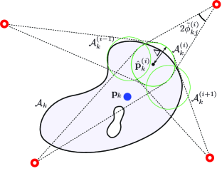
Figure 2: Illustration of the uncertainty model for WNL: $\big{\{}\mathcal{A}_{k}^{(i)}\big{\}}_{i\in\mathcal{I}_{k}}$ is a finite cover of the uncertainty region $\mathcal{A}_{k}$ for agent $k$, and each $\mathcal{A}_{k}^{(i)}$ is a circle with radius $\Delta$ centered at $\hat{\mathbf{p}}_{k}^{(i)}$.

Radar Network Localization

Similar to WNL, for unknown target position $\mathbf{p}_{0}\in\mathcal{A}^{(i)}$, the actual network parameters can be represented in the linear sets

$$\psi_{k} \in\Big{[}\,\hat{\psi}_{k}^{(i)}-\tilde{\psi}_{k}^{(i)}\,,\,\hat{\psi}_{k}^{(i)}+\tilde{\psi}_{k}^{(i)}\,\Big{]}=:\mathcal{B}_{1,k}^{(i)}$$

$$\varphi_{j} \in\Big{[}\,\hat{\varphi}_{j}^{(i)}-\tilde{\varphi}_{j}^{(i)}\,,\,\hat{\varphi}_{j}^{(i)}+\tilde{\varphi}_{j}^{(i)}\,\Big{]}=:\mathcal{B}_{2,j}^{(i)}$$

$${d}_{k} \in\Big{[}\,\hat{d}_{k}^{\,(i)}-\Delta\,,\,\hat{d}_{k}^{\,(i)}+\Delta\,\Big{]}\quad\text{and}\quad{\zeta}_{kj}\in\Big{[}\,\underline{\zeta}_{kj}^{(i)}\,,\,\overline{\zeta}_{kj}^{(i)}\,\Big{]}$$

where $\hat{\psi}_{k}^{(i)}$, $\hat{\varphi}_{k}^{(i)}$, and $\hat{d}_{k}^{\,(i)}$ are the nominal values of the topology parameters evaluated at $\hat{\mathbf{p}}_{0}^{(i)}$, $\tilde{\psi}_{k}^{(i)}=\arcsin(\Delta/\hat{d}_{k}^{\,(i)})$ and $\tilde{\varphi}_{j}^{(i)}=\arcsin(\Delta/\hat{d}_{j}^{\,(i)})$ are the angular uncertainty, and the last set characterizes the uncertainty of the RC from antennas $k$ to $j$ via the target. According to Proposition 2, we have the uncertainty sets for $\phi_{kj}$ and $\xi_{kj}$ as

$$\phi_{kj} \in\Big{[}\,\hat{\phi}_{kj}^{(i)}　-\tilde{\phi}_{kj}^{(i)}　\,,\,\hat{\phi}_{kj}^{(i)}+\tilde{\phi}_{kj}^{(i)}　\,\Big{]}=:\mathcal{B}_{kj}^{(i)}$$ (17)

$$\xi_{kj} \in\Big{[}\,\underline{\xi}_{kj}^{(i)}\,,\,\overline{\xi}_{kj}^{(i)}\,\Big{]}=:\mathcal{C}_{kj}^{(i)}$$ (18)

where $\hat{\phi}_{kj}^{(i)}=(\hat{\psi}_{k}^{(i)}+\hat{\varphi}_{j}^{(i)})/{2}$, $\tilde{\phi}_{kj}^{(i)}=(\tilde{\psi}_{k}^{(i)}+\tilde{\varphi}_{j}^{(i)})/{2}$, and the upper and lower bounds for $\xi_{kj}$ are given respectively by

$$\underline{\xi}_{kj}^{(i)} =\frac{4\,\underline{\zeta}_{kj}^{(i)}}{(\hat{d}_{k}^{\,(i)}+\Delta)^{2\beta}(\hat{d}_{j}^{\,(i)}+\Delta)^{2\beta}}\bigg{[}\min_{\phi\,\in\mathcal{D}_{kj}^{(i)}}\cos^{2}\phi\;\bigg{]}$$

$$\overline{\xi}_{kj}^{(i)} =\frac{4\,\overline{\zeta}_{kj}^{(i)}}{(\hat{d}_{k}^{\,(i)}-\Delta)^{2\beta}(\hat{d}_{j}^{\,(i)}-\Delta)^{2\beta}}\bigg{[}\max_{\phi\,\in\mathcal{D}_{kj}^{(i)}}\cos^{2}\phi\;\bigg{]}$$

in which $\mathcal{D}_{kj}^{(i)}:=\big{[}\,(\hat{\psi}_{k}^{(i)}-\hat{\varphi}_{j}^{(i)})/{2}-\tilde{\phi}_{kj}^{(i)}\,,\,(\hat{\psi}_{k}^{(i)}-\hat{\varphi}_{j}^{(i)})/{2}+\tilde{\phi}_{kj}^{(i)}\,\big{]}$. In summary, for the target’s position $\mathbf{p}_{0}\in\mathcal{A}$, the actual network parameters lie in the set

$$\{\psi_{k},\,\varphi_{j},\,\xi_{kj}\}_{k\in{\mathcal{N}_{\text{r}}},\,j\in{\mathcal{N}_{\text{t}}}}\in\bigcup_{i\in\mathcal{I}}\,\prod_{k\in{\mathcal{N}_{\text{r}}},\,j\in{\mathcal{N}_{\text{t}}}}\mathcal{B}_{1,k}^{(i)}\times\mathcal{B}_{2,j}^{(i)}\times\mathcal{C}_{kj}^{(i)}\,.$$

Remark 6

Note that the parameter uncertainty models for WNL and RNL can be converted to a common form, i.e., (14) and (17) for $\phi_{kj}$, and (15) and (18) for $\xi_{kj}$. Thus, we can develop robust formulations for the two scenarios under a unifying framework.

IV-B Robust Formulation

We now propose the robust counterparts of $\mathscr{P}_{\text{A}}$ and $\mathscr{P}_{\text{P}}$ that guarantee the localization requirement in the presence of parameter uncertainty. The worst-case SPEB for WNL due to parameter uncertainty (16) is

$$\mathcal{P}_{\text{R}}(\mathbf{p}_{k};\mathbf{x}) :=\max_{i\in\mathcal{I}_{k}}\,\mathcal{P}^{(i)}_{\text{R}}(\mathbf{p}_{k};\mathbf{x})$$

where $\mathcal{P}^{(i)}_{\text{R}}(\mathbf{p}_{k};\mathbf{x})$ is the worst-case SPEB in $\mathcal{A}_{k}^{(i)}$, given by

$$\mathcal{P}^{(i)}_{\text{R}}(\mathbf{p}_{k};\mathbf{x}):=\!\max_{\{(\phi_{kj},\,\xi_{kj})\in\mathcal{B}_{kj}^{(i)}\times\mathcal{C}_{kj}^{(i)}\}}\mathcal{P}(\mathbf{p}_{k};\mathbf{x})\,.$$

Hence, to guarantee the localization performance in the worst case, we introduce a new constraint $\mathcal{P}_{\text{R}}(\mathbf{p}_{k};\mathbf{x})\leq\varrho_{k}$ and formulate the robust power allocation problem for WNL as

$$\mathscr{P}_{\text{A-R}}:\;\;\min_{\{\mathbf{x}\}}\quad \mathbf{1}^{\text{T}}\,\mathbf{x}$$

s.t. $$\mathcal{P}^{(i)}_{\text{R}}(\mathbf{p}_{k};\mathbf{x})\leq\varrho_{k}\,,\;\;\forall\,k\in{\mathcal{N}_{\text{a}}}{\,,\,i\in\mathcal{I}_{k}}$$ (19)

$$c_{l}(\mathbf{x})\leq 0\,,\qquad\quad\;\;\,l=1,2,\ldots,L$$

where the localization requirement (19) is equivalent to $\mathcal{P}_{\text{R}}(\mathbf{p}_{k};\mathbf{x})\leq\varrho_{k}$ for $k\in{\mathcal{N}_{\text{a}}}$.

Similarly, we can obtain the worst-case SPEB for RNL as

$$\mathcal{P}_{\text{R}}(\mathbf{p}_{0};\mathbf{x}):=\max_{i\in\mathcal{I}_{k}}\,\mathcal{P}^{(i)}_{\text{R}}(\mathbf{p}_{0};\mathbf{x})$$

where

$$\mathcal{P}^{(i)}_{\text{R}}(\mathbf{p}_{0};\mathbf{x}):=\!\max_{\{(\psi_{k},\,\varphi_{j},\,\xi_{kj})\in\mathcal{B}_{1,k}^{(i)}\times\mathcal{B}_{2,j}^{(i)}\times\mathcal{C}_{kj}^{(i)}\}}\mathcal{P}(\mathbf{p}_{0};\mathbf{x})$$

and formulate the robust power allocation problem $\mathscr{P}_{\text{P-R}}$ by introducing the constraint $\mathcal{P}_{\text{R}}(\mathbf{p}_{0};\mathbf{x})\leq\varrho$. In the following we will focus on $\mathscr{P}_{\text{A-R}}$, and the analysis equally applies to $\mathscr{P}_{\text{P-R}}$.

We next convert (19) into an expression amenable for efficient optimization. Since the SPEB is a monotonically decreasing function in $\xi_{kj}$, the maximization over $\xi_{kj}\in\mathcal{C}^{(i)}_{kj}$ is achieved at $\xi_{kj}=\underline{\xi}_{kj}^{(i)}$. Thus, by Lemma 1, we can obtain

$$\mathcal{P}^{(i)}_{\text{R}}(\mathbf{p}_{k};\mathbf{x}) =\!\max_{\{\phi_{kj}\in\mathcal{B}^{(i)}_{kj}\}}\frac{4\cdot\mathbf{1}^{\text{T}}\,\underline{\mathbf{R}}_{k}^{(i)}\,\mathbf{x}}{\big{(}\mathbf{1}^{\text{T}}\,\underline{\mathbf{R}}_{k}^{(i)}\,\mathbf{x}\big{)}^{2}-\big{\|}[\,\mathbf{c}_{k}~{}~{}\mathbf{s}_{k}\,]^{\text{T}}\,\underline{\mathbf{R}}_{k}^{(i)}\,\mathbf{x}\big{\|}^{2}}$$ (20)

where $\underline{\mathbf{R}}_{k}^{(i)}=\text{diag}\big{\{}\underline{\xi}_{k1}^{(i)},\underline{\xi}_{k2}^{(i)},\ldots,\underline{\xi}_{k{{N}_{\text{b}}}}^{(i)}\big{\}}$. Unfortunately, the remaining maximization over $\{\phi_{kj}\}$ does not permit an explicit expression due to the intricate function.

To address the angular uncertainty, we propose sequential lower and upper bounds for $\mathcal{P}^{(i)}_{\text{R}}(\mathbf{p}_{k};\mathbf{x})$, both of which lead to efficient optimization programs. We denote $\mathcal{M}=\{0,1,\ldots,M-1\}$ where $M\in\mathbb{Z}_{+}$ and

$$B(\mathbf{x}):=\frac{1}{4}\,\mathcal{P}^{(i)}_{\text{R}}(\mathbf{p}_{k};\mathbf{x})\cdot\mathbf{1}^{\text{T}}\,\underline{\mathbf{R}}_{k}^{(i)}\,\mathbf{x}\,.$$

Proposition 4

For any given PAV $\mathbf{x}$ such that $\mathcal{P}^{(i)}_{\text{R}}(\mathbf{p}_{k};\mathbf{x})<\infty$, if $M\geq{\pi}\sqrt{B(\mathbf{x})}$, then $\mathcal{P}^{(i)}_{\text{R}}(\mathbf{p}_{k};\mathbf{x})$ is bounded below and above, respectively, by

$$\underline{\mathcal{P}}_{M}^{(i)}(\mathbf{p}_{k};\mathbf{x}) =\max_{m\in\mathcal{M}}\frac{4\cdot\mathbf{1}^{\text{T}}\,\underline{\mathbf{R}}_{k}^{(i)}\,\mathbf{x}}{(\mathbf{1}^{\text{T}}\,\underline{\mathbf{R}}_{k}^{(i)}\,\mathbf{x})^{2}-\big{(}\mathbf{h}_{k,m}^{(i)\,\text{T}}\,\underline{\mathbf{R}}_{k}^{(i)}\,\mathbf{x}\big{)}^{2}}$$ (21)

$$\overline{\mathcal{P}}_{M}^{(i)}(\mathbf{p}_{k};\mathbf{x}) =\max_{m\in\mathcal{M}}\frac{4\cdot\mathbf{1}^{\text{T}}\,\underline{\mathbf{R}}_{k}^{(i)}\,\mathbf{x}}{(\mathbf{1}^{\text{T}}\,\underline{\mathbf{R}}_{k}^{(i)}\,\mathbf{x})^{2}-\big{(}\mathbf{g}_{k,m}^{(i)\,\text{T}}\,\underline{\mathbf{R}}_{k}^{(i)}\,\mathbf{x}\big{)}^{2}}$$ (22)

where $\mathbf{h}_{k,m}^{(i)},\,\mathbf{g}_{k,m}^{(i)}\in\mathbb{R}^{{{N}_{\text{b}}}}$ with the $j$th elements given by

$$[\,\mathbf{h}_{k,m}^{(i)}\,]_{j} =\max_{|\epsilon|\leq 2\tilde{\phi}_{kj}^{(i)}}\,\cos(2\hat{\phi}_{kj}^{(i)}-\vartheta_{m}+\epsilon)$$

$$[\,\mathbf{g}_{k,m}^{(i)}\,]_{j} =\frac{1}{\cos({\pi}/{M})}\cdot[\,\mathbf{h}_{k,m}^{(i)}\,]_{j}$$

in which $\vartheta_{m}=(2m+1)\cdot\pi/M$ for $m\in\mathcal{M}$.

Proof:

See Appendix B. ∎

The proposed expressions parametrized by $M$ constitute a sequence of lower and upper bounds for the worst-case SPEB. We can substitute the worst-case SPEB in the localization requirement (19) by the lower and upper bounds, leading to the robust relaxation problems $\underline{\mathscr{P}}^{M}_{\text{A-R}}$ and $\overline{\mathscr{P}}^{M}_{\text{A-R}}$, respectively.

IV-C Asymptotically Optimal Algorithm

We first show that both the robust relaxation problems $\underline{\mathscr{P}}^{M}_{\text{A-R}}$ and $\overline{\mathscr{P}}^{M}_{\text{A-R}}$ can be transformed into SOCPs, and then derive the convergence rates of their solutions to that of the original problem $\mathscr{P}_{\text{A-R}}$.

Proposition 5

The problem $\overline{\mathscr{P}}^{M}_{\text{A-R}}$ is equivalent to the SOCP

$$\overline{\mathscr{P}}^{M}_{\text{A-R}}:\;\;\min_{\{\mathbf{x}\}}\quad \mathbf{1}^{\text{T}}\,\mathbf{x}$$

s.t. $${\big{\|}\mathbf{A}_{k,m}^{(i)}\,\underline{\mathbf{R}}_{k}^{(i)}\,{\mathbf{x}}+\mathbf{b}_{k}\big{\|}\leq\mathbf{1}^{\text{T}}\,\underline{\mathbf{R}}_{k}^{(i)}\,{\mathbf{x}}-2\varrho_{k}^{-1},}\,$$

$$\hskip 72.55452pt\forall\,m\in\mathcal{M}\,,\,k\in{\mathcal{N}_{\text{a}}}\,,\,{i\in\mathcal{I}_{k}}$$

$$c_{l}(\mathbf{x})\leq 0\,,\qquad\;\;\,l=1,2,\ldots,L$$

where $\mathbf{A}_{k,m}^{(i)}=\big{[}\,\mathbf{g}_{k,m}^{(i)}~{}~{}\mathbf{0}\,\big{]}^{\text{T}}$ and $\mathbf{b}_{k}=[\,0~{}~{}2\varrho_{k}^{-1}\,]^{\text{T}}$. Similarly, the problem $\underline{\mathscr{P}}^{M}_{\text{A-R}}$ is also equivalent to an SOCP by letting $\mathbf{A}_{k,m}^{(i)}=\big{[}\,\mathbf{h}_{k,m}^{(i)}~{}~{}\mathbf{0}\,\big{]}^{\text{T}}$ in the above constraints.

Proof:

For the upper bound case, we use the relaxed localization requirement $\overline{\mathcal{P}}^{(i)}_{M}(\mathbf{p}_{k};\mathbf{x})\leq\varrho_{k}$, which can be converted to the $M$ SOC forms

$${\big{\|}\mathbf{A}_{k,m}^{(i)}\,\underline{\mathbf{R}}_{k}^{(i)}\,{\mathbf{x}}+\mathbf{b}_{k}\big{\|}\leq\mathbf{1}^{\text{T}}\,\underline{\mathbf{R}}_{k}^{(i)}\,{\mathbf{x}}-2\varrho_{k}^{-1},\quad\forall\,m\in\mathcal{M}}$$

by using (22). The case for $\underline{\mathscr{P}}^{M}_{\text{A-R}}$ can be shown similarly. ∎

Remark 7

Although both relaxation formulations can be solved by SOCPs, $\overline{\mathscr{P}}^{M}_{\text{A-R}}$ is more desirable for implementation since it guarantees the localization requirement.

The next proposition proves that the gap between the lower and upper bounds for the worst-case SPEB, i.e., (21) and (22), converges to zero as $M\to\infty$.

Proposition 6

For any given PAV $\mathbf{x}\succeq\mathbf{0}$ such that $\mathcal{P}^{(i)}_{\text{R}}(\mathbf{p}_{k};\mathbf{x})<\infty$, if $M\geq\pi\sqrt{B(\mathbf{x})}$, then $\overline{\mathcal{P}}^{(i)}_{M}(\mathbf{p}_{k};\mathbf{x})\leq(1+C_{k,M}^{(i)})\,\underline{\mathcal{P}}^{(i)}_{M}(\mathbf{p}_{k};\mathbf{x})$, where

$$C_{k,M}^{(i)}=\frac{\sin^{2}({\pi}/{M})\,(B(\mathbf{x})-1)}{1-\sin^{2}({\pi}/{M})\,B(\mathbf{x})}\,.$$

Moreover, $C_{k,M}^{(i)}$ is monotonically decreasing with $M$ and

$$\lim_{M\to\infty}\frac{C_{k,M}^{(i)}}{M^{-2}}={\pi^{2}}(B(\mathbf{x})-1)\,.$$ (23)

Proof:

See Appendix C. ∎

Remark 8

This proposition implies that the gap between the lower and upper bounds goes to zero at the rate of $O(M^{-2})$. Using this result, we can show that both the solutions of $\overline{\mathscr{P}}^{M}_{\text{A-R}}$ and $\underline{\mathscr{P}}^{M}_{\text{A-R}}$ converge to that of the original problem at the rate of $O(M^{-2})$ as follows.

Proposition 7

Let $\mathbf{x}^{*}$, $\overline{\mathbf{x}}^{M}$, and $\underline{\mathbf{x}}^{M}$ be the optimal solutions of $\mathscr{P}_{\text{A-R}}$, $\overline{\mathscr{P}}^{M}_{\text{A-R}}$, and $\underline{\mathscr{P}}^{M}_{\text{A-R}}$, respectively. Then,

$$0 \leq{\mathbf{1}^{\text{T}}\overline{\mathbf{x}}^{M}-\mathbf{1}^{\text{T}}\mathbf{x}^{*}}\leq C_{M}\cdot\mathbf{1}^{\text{T}}\mathbf{x}^{*}$$

$$0 \leq\mathbf{1}^{\text{T}}\mathbf{x}^{*}-\mathbf{1}^{\text{T}}\underline{\mathbf{x}}^{M}\leq C_{M}\cdot\mathbf{1}^{\text{T}}\mathbf{x}^{*}$$

where $C_{M}=\max_{k\in{\mathcal{N}_{\text{a}}}}\max_{i\in\mathcal{I}_{k}}C_{k,M}^{(i)}$ converges to zero at the rate of $O(M^{-2})$.

Proof:

See Appendix D. ∎

Remark 9

Since the solutions of the proposed relaxation problems converge to that of the original problem at the rate of $O(M^{-2})$, the optimal solution of $\mathscr{P}_{\text{A-R}}$ can be approximated by that of $\overline{\mathscr{P}}^{M}_{\text{A-R}}$ with a small value of $M$. For example, our simulation results show that its performance loss is less than 2% when $M\geq 16$. On the other hand, note that the number of SOC constraints of the relaxation problems increases linearly with $M$, resulting in the increase in computational complexity at ${O}(M^{{3}/{2}})$ [47]. This gives an important guideline on the performance versus complexity tradeoff for the robust power allocation algorithms in practice.

While the proposed SOCP-based algorithms are asymptotically optimal, we next develop efficient near-optimal algorithms, which involve only a few SOC constraints, for power allocation in dynamic networks with limited computational capability.

IV-D Efficient Algorithms

We next propose a relaxation method to address the angular uncertainty involved in the worst-case SPEB, leading to efficient SOCP-based algorithms. For notational convenience, we omit the superscript $(i)$ in this section.

Since only the denominator in (20) is a function of $\phi_{kj}$, we derive an upper bound for $\mathcal{P}_{\text{R}}(\mathbf{p}_{k};\mathbf{x})$ by finding a lower bound for the denominator. Denote the vectors $\hat{\mathbf{c}}_{k}=\mathbf{c}(2\hat{\boldsymbol{\phi}}_{k})$ and $\hat{\mathbf{s}}_{k}=\mathbf{s}(2\hat{\boldsymbol{\phi}}_{k})$, where $\hat{\boldsymbol{\phi}}_{k}=[\,\hat{\phi}_{k1}~{}~{}\hat{\phi}_{k2}~{}~{}\cdots~{}~{}\hat{\phi}_{k{{N}_{\text{b}}}}\,]^{\text{T}}$; and $\tilde{\mathbf{s}}_{k},\,\tilde{\mathbf{c}}_{k}\in\mathbb{R}^{{{N}_{\text{b}}}}$ with $j$th elements given, respectively, by

$$[\,\tilde{\mathbf{s}}_{k}\,]_{j} =\max_{|\epsilon|\leq\tilde{\phi}_{kj}}\big{|}2\sin(2\hat{\phi}_{kj}+\epsilon)\sin\epsilon\,\big{|}$$

$$[\,\tilde{\mathbf{c}}_{k}\,]_{j} =\max_{|\epsilon|\leq\tilde{\phi}_{kj}}\big{|}2\cos(2\hat{\phi}_{kj}+\epsilon)\sin\epsilon\,\big{|}\,.$$

Proposition 8

Let

$$\mathcal{P}_{\text{U}}(\mathbf{p}_{k};\mathbf{x})=\!\max_{e_{1},\,e_{2}=\pm 1}\!\frac{4\cdot\mathbf{1}^{\text{T}}\,\underline{\mathbf{R}}_{k}\,\mathbf{x}}{\big{(}\mathbf{1}^{\text{T}}\,\underline{\mathbf{R}}_{k}\,\mathbf{x}\big{)}^{2}-\big{\|}\hat{\mathbf{A}}_{k}^{(e_{1},\,e_{2})}\,\underline{\mathbf{R}}_{k}\,\mathbf{x}\big{\|}^{2}}$$ (24)

where $\hat{\mathbf{A}}_{k}^{(e_{1},\,e_{2})}=[\,(\hat{\mathbf{c}}_{k}+e_{1}\tilde{\mathbf{s}}_{k})~{}~{}(\hat{\mathbf{s}}_{k}+e_{2}\tilde{\mathbf{c}}_{k})~{}~{}\mathbf{0}\,]^{\text{T}}$. Then $\mathcal{P}_{\text{R}}(\mathbf{p}_{k};\mathbf{x})\leq\mathcal{P}_{\text{U}}(\mathbf{p}_{k};\mathbf{x})$, provided that $\mathcal{P}_{\text{U}}(\mathbf{p}_{k};\mathbf{x})>0$.

Proof:

See Appendix E. ∎

Since $\mathcal{P}_{\text{U}}(\mathbf{p}_{k};\mathbf{x})$ is an upper bound for the worst-case SPEB, we can relax the constraint (19) in $\mathscr{P}_{\text{A-R}}$ by

$$0<\mathcal{P}_{\text{U}}(\mathbf{p}_{k};\mathbf{x})\leq\varrho_{k}$$

which can be converted to the set of four SOC constraints

$$\big{\|}\hat{\mathbf{A}}_{k}^{(e_{1},\,e_{2})}\,\underline{\mathbf{R}}_{k}\,{\mathbf{x}}+{\mathbf{b}}_{k}\big{\|}\leq\mathbf{1}^{\text{T}}\,\underline{\mathbf{R}}_{k}\,{\mathbf{x}}-2\varrho_{k}^{-1},\;\;e_{1},e_{2}=\pm 1$$ (25)

where ${\mathbf{b}}_{k}=[\,0~{}~{}0~{}~{}2\varrho_{k}^{-1}\,]^{\text{T}}$. Hence, by replacing each constraint (19) in $\mathscr{P}_{\text{A-R}}$ with the four constraints (25), we obtain an efficient SOCP $\mathscr{P}_{\text{A-R}}^{\text{SOCP}}$ as a relaxation for the robust power allocation problem.

Remark 10

Comparing (25) of $\mathscr{P}_{\text{A-R}}^{\text{SOCP}}$ with (13) of $\mathscr{P}_{\text{A}}^{\text{SOCP}}$, one can observe that the proposed robust relaxation retains the SOC form as its nonrobust counterpart. Furthermore, when the parameter uncertainty vanishes, $\tilde{\mathbf{s}}_{k},\,\tilde{\mathbf{c}}_{k}\to\mathbf{0}$ and thus $\mathscr{P}_{\text{A-R}}^{\text{SOCP}}$ reduces to $\mathscr{P}_{\text{A}}^{\text{SOCP}}$ as (25) reduces to (13).

Similar to the WNL case, we can derive an upper bound for the worst-case SPEB in the form of (24) and formulate a corresponding robust relaxation problem for the RNL case. Specifically for RNL, since the ${{N}_{\text{r}}}{N_{\text{t}}}$ angles $\{\phi_{kj}\}_{k\in{\mathcal{N}_{\text{r}}},\,j\in{\mathcal{N}_{\text{t}}}}$ in (5) are generated only by the ${{N}_{\text{r}}}+{N_{\text{t}}}$ angles $\{\psi_{k},\,\varphi_{j}\}_{k\in{\mathcal{N}_{\text{r}}},\,j\in{\mathcal{N}_{\text{t}}}}$, we can obtain a tighter bound by addressing the angular uncertainty in the transmit and receive antennas separately. In other words, we start from the uncertainty set $(\psi_{k},\,\varphi_{j})\in\mathcal{B}_{1,k}\times\mathcal{B}_{2,j}$ instead of $\phi_{kj}\in\mathcal{B}_{kj}$.

Denote the matrix $\underline{\mathbf{R}}_{\Sigma}=　\sum_{k=1}^{{{N}_{\text{r}}}}\underline{\mathbf{R}}_{k}$, where $\underline{\mathbf{R}}_{k}=\text{diag}\big{\{}\underline{\xi}_{k1},\underline{\xi}_{k2},\ldots,\underline{\xi}_{k{N_{\text{t}}}}\big{\}}$; the vector $\hat{\boldsymbol{\varphi}}=[\,\hat{\varphi}_{1}~{}~{}\hat{\varphi}_{2}~{}~{}\cdots~{}~{}\hat{\varphi}_{N_{\text{t}}}\,]^{\text{T}}$; the vectors

$$\hat{\mathbf{c}} =\underline{\mathbf{R}}_{\Sigma}^{-1}\cdot\sum_{k=1}^{{{N}_{\text{r}}}}\underline{\mathbf{R}}_{k}^{\text{T}}\,\mathbf{c}(\hat{\boldsymbol{\varphi}}+\hat{\psi}_{k}\mathbf{1})$$

$$\hat{\mathbf{s}} =\underline{\mathbf{R}}_{\Sigma}^{-1}\cdot\sum_{k=1}^{{{N}_{\text{r}}}}\underline{\mathbf{R}}_{k}^{\text{T}}\,\mathbf{s}(\hat{\boldsymbol{\varphi}}+\hat{\psi}_{k}\mathbf{1})$$

$\tilde{\mathbf{s}}=\underline{\mathbf{R}}_{\Sigma}^{-1}\cdot\sum_{k=1}^{{{N}_{\text{r}}}}\underline{\mathbf{R}}_{k}^{\text{T}}\,\tilde{\mathbf{s}}_{k}$, and $\tilde{\mathbf{c}}=\underline{\mathbf{R}}_{\Sigma}^{-1}\cdot\sum_{k=1}^{{{N}_{\text{r}}}}\underline{\mathbf{R}}_{k}^{\text{T}}\,\tilde{\mathbf{c}}_{k}$, where $\tilde{\mathbf{s}}_{k},\,\tilde{\mathbf{c}}_{k}\in\mathbb{R}^{{N_{\text{t}}}}$ with $j$th elements given, respectively, by

$$[\,\tilde{\mathbf{s}}_{k}\,]_{j} =\max_{|\epsilon|\leq(\tilde{\psi}_{k}+\tilde{\varphi}_{j})/2}\big{|}2\sin(\hat{\psi}_{k}+\hat{\varphi}_{j}+\epsilon)\sin\epsilon\,\big{|}$$

$$[\,\tilde{\mathbf{c}}_{k}\,]_{j} =\max_{|\epsilon|\leq(\tilde{\psi}_{k}+\tilde{\varphi}_{j})/2}\big{|}2\cos(\hat{\psi}_{k}+\hat{\varphi}_{j}+\epsilon)\sin\epsilon\,\big{|}\,.$$

Proposition 9

Let

$$\mathcal{P}_{\text{U}}(\mathbf{p}_{0};\mathbf{x})=\!\max_{e_{1},\,e_{2}=\pm 1}\!\frac{4\cdot\mathbf{1}^{\text{T}}\,\underline{\mathbf{R}}_{\Sigma}\,\mathbf{x}}{(\mathbf{1}^{\text{T}}\,\underline{\mathbf{R}}_{\Sigma}\,\mathbf{x})^{2}-\big{\|}\hat{\mathbf{A}}^{(e_{1},\,e_{2})}\,\underline{\mathbf{R}}_{\Sigma}\,\mathbf{x}\big{\|}^{2}}$$

where $\hat{\mathbf{A}}^{(e_{1},\,e_{2})}=[\,(\hat{\mathbf{c}}+e_{1}\tilde{\mathbf{s}})~{}~{}(\hat{\mathbf{s}}+e_{2}\tilde{\mathbf{c}})~{}~{}\mathbf{0}\,]^{\text{T}}$. Then $\mathcal{P}_{\text{R}}(\mathbf{p}_{0};\mathbf{x})\leq\mathcal{P}_{\text{U}}(\mathbf{p}_{0};\mathbf{x})$, provided that $\mathcal{P}_{\text{U}}(\mathbf{p}_{0};\mathbf{x})>0$.

Proof:

The proof follows a similar approach of Proposition 8. ∎

Remark 11

The upper bound $\mathcal{P}_{\text{U}}(\mathbf{p}_{0};\mathbf{x})$ for the worst-case SPEB can be used as a relaxation for the robust power allocation problem in RNL, leading to an efficient SOCP $\mathscr{P}_{\text{P-R}}^{\text{SOCP}}$. Such a relaxation not only retains the SOC form but also naturally reduces to its nonrobust counterpart when the parameter uncertainty vanishes.

V Discussions

In this section, we provide discussions on several related issues, including 1) prior knowledge of the network parameters, 2) broader applications of the SPEB properties, and 3) the achievability of the SPEB.

V-A Prior Knowledge

Since the prior knowledge of the network parameters, if available, can be exploited to improve the localization accuracy, we next investigate the power allocation problem for WNL with prior knowledge of the network parameters. The discussion is also applicable to RNL.

The EFIM for the case with prior knowledge is a $2\times 2$ matrix given by [20]

$$\mathbf{J}_{\text{e}}(\mathbf{p}_{k};\mathbf{x})=\mathbf{J}_{0}(\mathbf{p}_{k})+\sum_{j\in{\mathcal{N}_{\text{b}}}}x_{j}\cdot\mathbf{J}_{kj}$$ (26)

where $\mathbf{J}_{0}(\mathbf{p}_{k})\in\mathbb{S}_{+}^{2}$ is the FIM for the prior position knowledge of agent $k$ and $\mathbf{J}_{kj}\in\mathbb{S}_{+}^{2}$ is given by

$$\mathbf{J}_{kj}=\mathbb{E}_{\mathbf{r},\boldsymbol{\theta}}\left\{{\xi}_{kj}\,\mathbf{J}_{\text{r}}({\phi}_{kj})\right\}$$ (27)

in which the expectation is taken with respect to the agent $k$’s prior position knowledge, the prior channel knowledge between agent $k$ and anchor $j$, and the observation noise.

The SPEB $\mathcal{P}(\mathbf{p}_{k};\mathbf{x})$ for the case with prior knowledge can be obtained from the EFIM (26). By employing such SPEB, we can formulate the power allocation problem and its robust counterpart, denoted by $\widetilde{\mathscr{P}}_{\text{A}}$ and $\widetilde{\mathscr{P}}_{\text{A-R}}$, in the analogous way as $\mathscr{P}_{\text{A}}$ and $\mathscr{P}_{\text{A-R}}$, respectively.

Proposition 10

The problems $\widetilde{\mathscr{P}}_{\text{A}}$ and $\widetilde{\mathscr{P}}_{\text{A-R}}$ can be transformed into SOCPs.

Proof:

See Appendix F. ∎

Remark 12

The proposition shows that the power allocation problems $\widetilde{\mathscr{P}}_{\text{A}}$ and $\widetilde{\mathscr{P}}_{\text{A-R}}$ for the case with prior knowledge can also be transformed into SOCPs. Moreover, these problems reduce to $\mathscr{P}_{\text{A}}$ and $\mathscr{P}_{\text{A-R}}$ when the prior knowledge vanishes since $\mathbf{J}_{0}(\mathbf{p}_{k})=\mathbf{0}$ in (26) and the expectation in (27) is only with respect to $\mathbf{r}$.

Since the prior position knowledge $\mathbf{J}_{0}(\mathbf{p}_{k})\succeq 0$ provides additional information to the EFIM compared to the case without such knowledge, less transmit power is required to achieve the same localization requirement. In particular, if $\text{tr}\{\mathbf{J}_{0}^{-1}(\mathbf{p}_{k})\}\leq\varrho_{k}$ for all $k\in{\mathcal{N}_{\text{a}}}$, then all the agents have met their localization requirement and the anchors do not need to transmit ranging signals until $\text{tr}\{\mathbf{J}_{0}^{-1}(\mathbf{p}_{k})\}>\varrho_{k}$ for some $k$ (e.g., due to the agent movement).

V-B Applications of SPEB Properties

Lemma 1 shows two important properties of the SPEB, based on which we transformed the power allocation formulations $\mathscr{P}_{\text{A}}$ and $\mathscr{P}_{\text{P}}$ into SOCPs in Section III-B. Such properties also permit efficient algorithms for other power allocation problems in network localization as discussed in the following.

First, the methods developed in this paper are applicable to other formulations of the power allocation problems. For instance, minimizing the maximum localization error of the agents for a given power constraint can be formulated as

$$\max_{\{\mathbf{x},\,\rho\}}\quad \rho$$

s.t. $$\mathbf{1}^{\text{T}}\,\mathbf{x}\leq P_{\text{tot}}$$

$$\mathcal{P}(\mathbf{p}_{k};\mathbf{x})\leq\rho^{-1},\quad\forall\,k\in{\mathcal{N}_{\text{a}}}$$

$$c_{l}(\mathbf{x})\leq 0\,,\qquad\quad\;\;l=1,2,\ldots,L$$

where $P_{\text{tot}}$ denotes the total power constraint. Following the derivation in Proposition 3, one can see that $\mathcal{P}(\mathbf{p}_{k};\mathbf{x})\leq\rho^{-1}$ can be converted to an SOC form in $\mathbf{x}$ and $\rho$, and thus the above problem is equivalent to an SOCP. Moreover, a similar SOCP formulation can be obtained if the objective is to minimize the total localization errors of the agents for a given power constraint.

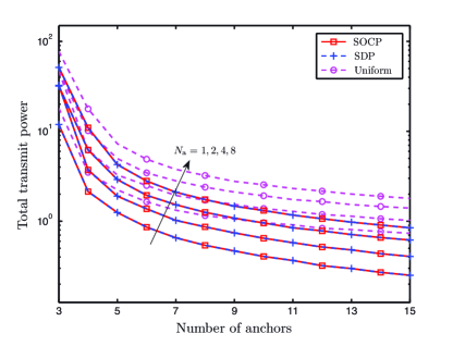
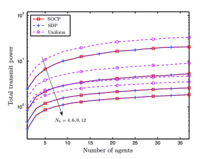
Figure 3: Total transmit power as a function of the number of anchors (a) and agents (b): (a) networks with 1, 2, 4, and 8 agents; (b) networks with 4, 6, 9, and 12 anchors.

Second, we can show by the SPEB properties that the optimal localization performance can be achieved by activating only three anchors for the single-agent case with no individual power constraints [45]. The same claim also applies to RNL, i.e., only three transmit antennas need to be activated for optimal target localization. This finding for the single-agent case provides important insights into the power allocation problem for network localization: only a few anchors or transmit antennas need to be activated for the optimal localization performance.

V-C Achievability of SPEB

The SPEB is based on the information inequality and hence characterizes the lower bound for the mean squared position errors, which is asymptotically achievable by the maximum likelihood estimators in high SNR regimes (over $10\sim 15$ dB) [48, 24, 5]. Wireless networks and radar networks for high-accuracy localization need to operate in such regimes, which can be realized for example by repeated transmissions, coded sequences, or spread spectrum. Hence, the SPEB can be used as the performance metric for the design and analysis of power allocation for a broad range of high-accuracy localization applications. Although the performance measure SPEB is less meaningful in low SNR regimes, the methods and results based on the SPEB can serve as a design guideline for localization power optimization.

VI Numerical Results

In this section, we evaluate the performance of the proposed power allocation algorithms. For WNL, we consider a 2-D network where the anchors and agents are randomly distributed in a region of size $D\times D$. Without loss of generality, the localization requirement for the agents is normalized to $\varrho_{k}=1$, $\forall\,k\in{\mathcal{N}_{\text{a}}}$. The RCs $\{\zeta_{kj}\}_{k\in{\mathcal{N}_{\text{a}}},\,j\in{\mathcal{N}_{\text{b}}}}$ are modeled as independent Rayleigh random variables with mean $\mu_{\zeta}$. We compare the normalized required total transmit power $P_{\text{tot}}={\mu_{\zeta}}/{D^{2\beta}}\cdot\mathbf{1}^{\text{T}}\,\mathbf{x}$ to meet the localization requirement by different algorithms. Similarly for RNL, the antennas and the target are randomly distributed in a region of size $D\times D$. The localization requirement for the target is normalized to $\varrho=1$. The RCs $\{\zeta_{kj}\}_{k\in{\mathcal{N}_{\text{r}}},\,j\in{\mathcal{N}_{\text{t}}}}$ are modeled as independent Rayleigh RVs with mean $\mu_{\zeta}$. We also compare the normalized required total transmit power $P_{\text{tot}}={\mu_{\zeta}}/{D^{4\beta}}\cdot\mathbf{1}^{\text{T}}\,\mathbf{x}$.

VI-A Wireless Network Localization

We first compare the performance of SOCP-based, SDP-based, and uniform power allocation algorithms for WNL with perfect network parameters. The required total transmit power as a function of the number of anchors and agents is shown in Fig. 3. First, for a given number of agents, the required power decreases with the number of anchors as shown in Fig. 3 since more degrees of freedom are available for power allocation. On the other hand, for a given number of anchors, the required power increases with the number of agents as shown in Fig. 3 since more constraints are imposed for the localization requirement of additional agents. Second, the SOCP- and SDP-based algorithms yield identical solutions as they both achieve the global optimum, significantly outperforming the uniform allocation algorithm, e.g., reducing the required power by more than $40\%$. Third, the concavity of the curves in Fig. 3 implies that less incremental power is required for additional agents as the number of agents increases. This agrees with the intuition because due to anchor broadcasting, each new agent can utilize the transmit power intended for the existing agents and thus less additional power is needed to meet its localization requirement.

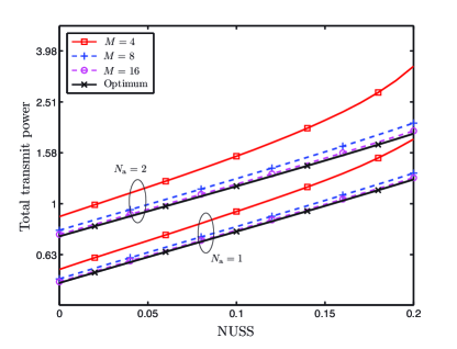
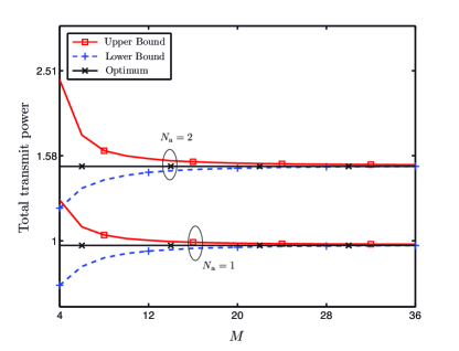
Figure 4: Total transmit power based on asymptotically optimal algorithms as a function of the NUSS (a) and parameter $M$ (b) for networks with eight anchors and one/two agents: (a) $M=$4, 8, 16; (b) NUSS$=$ 0.15.

We next consider the case with network parameter uncertainty and compare the solutions of the asymptotically optimal algorithms to the optimal solution for a network with eight anchors and one/two agents. We denote $\varepsilon=2\Delta/D$ as the normalized uncertainty set size (NUSS), where the true position of each agent can be anywhere in the circle centered at its nominal position with radius $\Delta$. Thus, the maximum uncertainty in $d_{kj}$ is $\varepsilon D/2$ and in ${\phi}_{kj}$ is $\arcsin(\varepsilon D/2d_{kj})$. The required total transmit power as a function of the NUSS and parameter $M$ is shown in Fig. 4. First, the required power increases with the NUSS as shown in Fig. 4. This is because a larger NUSS translates to a larger range of possible network parameters and consequently a larger worst-case SPEB, thus requiring more transmit power to guarantee the localization requirement. Second, Fig. 4 depicts the convergence behaviors of $\overline{\mathscr{P}}^{M}_{\text{A-R}}$ and $\underline{\mathscr{P}}^{M}_{\text{A-R}}$ as a function of $M$ for the NUSS equal to 0.15. In particular, the solutions of both problems approach the optimal solution as $M$ increases, which agrees with Proposition 7. For example, when ${N_{\text{a}}}=1$, the gaps between the solutions of $\overline{\mathscr{P}}^{M}_{\text{A-R}}$ and the optimal solution are about 30%, 5%, and 2% for $M=4$, $8$, and $16$, respectively.

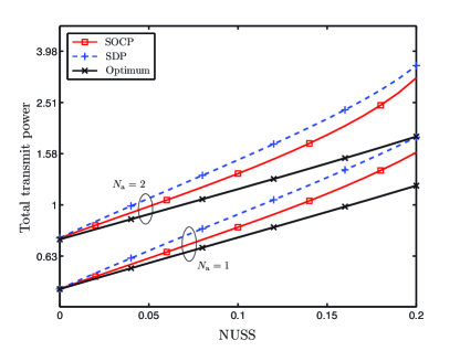
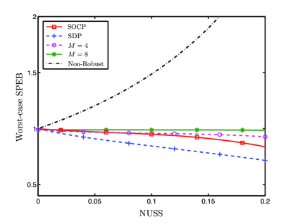
Figure 5: Total transmit power (a) and worst-case SPEB (b) as a function of the NUSS: (a) networks with eight anchors and one/two agents; (b) a network with eight anchors and one agent.

We then evaluate the performance of the proposed efficient SOCP-based algorithm for a network with eight anchors and one/two agents. Figure 5 shows the required total transmit power and the worst-case SPEB as a function of the NUSS. First, all the algorithms require more power when the NUSS increases, as shown in Fig. 5. Second, the SOCP-based algorithm outperforms the SDP-based algorithm developed in [44], e.g., the gaps between their solutions and the optimal solution are 15% and 33%, respectively, for the NUSS equal to 0.15. Third, the gap between the solution of the SOCP-based algorithm and the optimal solution increases with the NUSS and vanishes when the NUSS is zero. This performance loss is expected since larger uncertainty requires more conservative relaxation. Fourth, as shown in Fig. 5, the worst-case SPEB by the nonrobust algorithm increases with the NUSS, significantly violating the localization requirement. This manifests the necessity of robust formulations to guarantee the localization requirement in the presence of parameter uncertainty.

VI-B Radar Network Localization

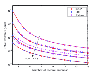
Figure 6: Total transmit power as a function of the number of transmit antennas: networks with 1, 2, 4, and 8 receive antennas.

We next compare the performance of the SOCP-based, SDP-based, and uniform power allocation algorithms for RNL with perfect network parameters. The required total transmit power as a function of the number of transmit and receive antennas is shown in Fig. 6. First, for a given number of receive antennas, the required power decreases with the number of transmit antennas since more degrees of freedom are available for power allocation. On the other hand, for a given number of transmit antennas, the required power decreases with the number of receive antennas since more independent copies of signals are received. Second, the SOCP- and SDP-based algorithms yield identical solutions, significantly outperforming the uniform allocation when there are more than one transmit antenna, e.g., reducing the required power by 30% when there are four transmit antennas. Third, the performance improvement of the SOCP-based algorithm over the uniform allocation increases with the number of transmit antennas. In particular, there is no improvement for the case with one transmit antenna (i.e., the three curves overlap), while the SOCP-based algorithm reduces over 70% of the power when there are eight transmit antennas. Fourth, for a given number of transmit antennas, the required power reduction by the SOCP-based algorithm does not depend on the number of receive antennas, e.g., the reduction is 15%, 35%, and 50% for 2, 4, and 8 transmit antennas, respectively, regardless of the number of receive antennas. This implies that different numbers of receive antennas provide the same gain from independent signals for optimal and uniform power allocation.

We finally compare the solution of the proposed efficient SOCP-based algorithm to the optimal solution for a network with $6\times 2$, $6\times 6$, and $6\times 10$ transmit-receive antenna pairs. Figure 7 shows the required total transmit power as a function of the NUSS, from which we can make similar observations as those for the WNL case. First, all the algorithms require more power when the NUSS increases, as shown in Fig. 7. Second, the SOCP-based algorithm outperforms the SDP-based algorithm, e.g., the gaps between their solutions and the optimal solution are 12% and 35%, respectively, for the NUSS equal to 0.15. Third, the gap between the solution of the SOCP-based algorithm to the optimal solution increases with the NUSS and vanishes when the NUSS is zero.

VII Conclusion

In this paper, we established a unifying optimization framework for power allocation in both active and passive localization networks. We first determined two functional properties, i.e., convexity and low rank, of the SPEB. Based on these properties, we showed that the power allocation problems can be transformed into SOCPs, which are amenable for efficient optimization. Moreover, we proposed a robust formulation to tackle the uncertainty in network parameters, and then developed both asymptotically optimal and efficient near-optimal algorithms. These algorithms retain the SOCP form and naturally reduce to their nonrobust counterparts when the uncertainty vanishes. Our simulation results showed that the proposed power allocation algorithms significantly outperform the uniform allocation algorithm. The results also manifested the necessity of the robust formulation to guarantee the localization requirement in the presence of parameter uncertainty. The performance comparison of the asymptotically optimal and efficient near-optimal algorithms provides important insights into robust algorithm design under the performance versus complexity tradeoffs.

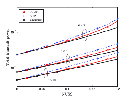
Figure 7: Total transmit power as a function of the NUSS: networks with $6\times 2$, $6\times 6$, and $6\times 10$ transmit-receive antennas.

Appendix A Proof of Lemma 1

Proof:

Note that $\mathcal{P}(\mathbf{p_{k}};\mathbf{x})=\text{tr}\{\mathbf{J}_{\text{e}}^{-1}(\mathbf{p}_{k};\mathbf{x})\}$ is a non-increasing convex function of $\mathbf{J}_{\text{e}}(\mathbf{p}_{k};\mathbf{x})\in\mathbb{S}_{+}^{n}$ [35] and $\mathbf{J}_{\text{e}}(\mathbf{p}_{k};\mathbf{x})$ is a linear function of $\mathbf{x}\succeq\mathbf{0}$. By the convexity property of the composition functions, we can conclude that the SPEB is a convex function of $\mathbf{x}\succeq\mathbf{0}$.

We next show that the topology matrix $\boldsymbol{\Lambda}_{k}$ can be written as (12). Based on (3) and (4), we can derive the SPEB of agent $k$ as (11), where the elements of $\boldsymbol{\Lambda}_{k}$ can be written as

$$[\boldsymbol{\Lambda}_{k}]_{ij} =2\sin^{2}(\phi_{ki}-\phi_{kj})$$

$$\stackrel{{\scriptstyle\text{(a)}}}{{=}}1-\cos(2\phi_{ki})\cos(2\phi_{kj})-\sin(2\phi_{ki})\sin(2\phi_{kj})$$

where (a) follows from the sum and difference formulas of the trigonometric functions. After some rearrangement, we can obtain the expression (12) for $\boldsymbol{\Lambda}_{k}$. We omit the proof for the RNL case since it can be derived in a similar way. ∎

Appendix B Proof of Proposition 4

We first present the following lemma for the proof of Proposition 4.

Lemma 2 (Finite Projection Bound)

For any $\mathbf{y}\succeq\mathbf{0}_{{{N}_{\text{b}}}}$, let $S(\mathbf{y}):=\max_{\{\phi_{kj}\in\mathcal{B}^{(i)}_{kj}\}}\big{\|}\sum_{j\in{\mathcal{N}_{\text{b}}}}y_{j}\,\mathbf{u}(2\phi_{kj})\big{\|}$, then

$$0\leq\max_{m\in\mathcal{M}}\,\big{\{}\mathbf{h}_{k,m}^{(i)\,\text{T}}\,\mathbf{y}\big{\}} \leq S(\mathbf{y})\leq\max_{m\in\mathcal{M}}\,\big{\{}\mathbf{g}_{k,m}^{(i)\,\text{T}}\,\mathbf{y}\big{\}}\,.$$

Proof:

Note that for a given $\mathbf{y}\succeq\mathbf{0}$,

$$S(\mathbf{y}) =\max_{\vartheta\in[\,0,\,2\pi)}\max_{\{\phi_{kj}\in\mathcal{B}^{(i)}_{kj}\}}\mathbf{u}^{\text{T}}(\vartheta)\cdot\sum_{j\in{\mathcal{N}_{\text{b}}}}y_{j}\,\mathbf{u}(2\phi_{kj})$$

$$\stackrel{{\scriptstyle\text{(a)}}}{{=}}\max_{\vartheta\in[\,0,\,2\pi)}\sum_{j\in{\mathcal{N}_{\text{b}}}}y_{j}\max_{|\epsilon_{kj}|\leq 2\tilde{\phi}_{kj}^{(i)}}\cos(2\hat{\phi}_{kj}^{(i)}+\epsilon_{kj}-\vartheta)\!$$ (28)

where (a) follows from ${\phi}_{kj}=\hat{\phi}_{kj}^{(i)}+\epsilon_{kj}/2$ in which $|\epsilon_{kj}|\leq 2\tilde{\phi}_{kj}^{(i)}$ according to (14).

For the lower bound, since $\{\vartheta_{m}:m\in\mathcal{M}\}\subset[\,0,\,2\pi)$, the maximum over $\vartheta\in[\,0,\,2\pi)$ in (28) can be bounded below by the maximum over $\vartheta\in\{\vartheta_{m}:m\in\mathcal{M}\}$, and thus

$$S(\mathbf{y}) \geq\max_{m\in\mathcal{M}}\,\sum_{j\in{\mathcal{N}_{\text{b}}}}y_{j}\max_{|\epsilon_{kj}|\leq 2\tilde{\phi}_{kj}^{(i)}}\cos(2\hat{\phi}_{kj}^{(i)}+\epsilon_{kj}-\vartheta_{m})$$

$$=\max_{m\in\mathcal{M}}\,\big{\{}\mathbf{h}_{k,m}^{(i)\,\text{T}}\,\mathbf{y}\big{\}}\,.$$

For the upper bound, let $\vartheta^{*}$ and $\{\epsilon_{kj}^{*}\}$ be the optimal angles that achieve the maximum in (28), and let $m^{*}\in\mathcal{M}$ such that $\vartheta^{*}\in[\,\vartheta_{m^{*}}-{\pi}/{M},\,\vartheta_{m^{*}}+{\pi}/{M})$. Then, by the definition of $S(\mathbf{y})$, we have

$$S(\mathbf{y})\,\mathbf{u}(\vartheta^{*})=\sum_{j\in{\mathcal{N}_{\text{b}}}}y_{j}\mathbf{u}(2\hat{\phi}_{kj}^{(i)}+\epsilon_{kj}^{*})$$

and multiplying both sides by $\mathbf{u}^{\text{T}}(\vartheta_{m^{*}})$ leads to

$$S(\mathbf{y}) \cos(\vartheta^{*}-\vartheta_{m^{*}})$$

$$=\sum_{j\in{\mathcal{N}_{\text{b}}}}y_{j}\cos(2\hat{\phi}_{kj}^{(i)}+\epsilon_{kj}^{*}-\vartheta_{m^{*}})$$

$$\stackrel{{\scriptstyle\text{(a)}}}{{\leq}}\sum_{j\in{\mathcal{N}_{\text{b}}}}y_{j}\!\max_{|\epsilon_{kj}|\leq 2\tilde{\phi}_{kj}^{(i)}}\cos(2\hat{\phi}_{kj}^{(i)}+\epsilon_{kj}-\vartheta_{m^{*}})$$

$$=\mathbf{h}_{k,m^{*}}^{(i)\,\text{T}}\,\mathbf{y}\leq\max_{m\in\mathcal{M}}\,\big{\{}\mathbf{h}_{k,m}^{(i)\,\text{T}}\,\mathbf{y}\big{\}}$$

where (a) follows from $|\epsilon_{kj}^{*}|\leq 2\tilde{\phi}_{kj}^{(i)}$. On the other hand, since $|\vartheta^{*}-\vartheta_{m^{*}}|\leq\pi/M$, we have

$$S(\mathbf{y})\,\cos(\vartheta^{*}-\vartheta_{m^{*}})\geq S(\mathbf{y})\,\cos(\pi/M)$$

which in combination with the above leads to

$$S(\mathbf{y})\leq\max_{m\in\mathcal{M}}\,\big{\{}\mathbf{g}_{k,m}^{(i)\,\text{T}}\,\mathbf{y}\big{\}}\,.$$

Finally, note that

$$\sum_{m\in\mathcal{M}}\mathbf{h}_{k,m}^{(i)\,\text{T}}\,\mathbf{y} =\sum_{j\in{\mathcal{N}_{\text{b}}}}y_{j}\!\!\sum_{m\in\mathcal{M}}\max_{\{|\epsilon_{kj}|\leq 2\tilde{\phi}_{kj}^{(i)}\}}\!\cos(2\hat{\phi}_{kj}^{(i)}+\epsilon_{kj}-\vartheta_{m})$$

$$\geq\sum_{j\in{\mathcal{N}_{\text{b}}}}y_{j}\sum_{m\in\mathcal{M}}\cos(2\hat{\phi}_{kj}^{(i)}-\vartheta_{m})=0$$

which implies that $\max_{m\in\mathcal{M}}\,\big{\{}\mathbf{h}_{k,m}^{(i)\,\text{T}}\,\mathbf{y}\big{\}}\geq 0$. ∎

We next give the proof of the proposition.

Proof:

Let $\mathbf{y}=\underline{\mathbf{R}}_{k}^{(i)}\,\mathbf{x}$. First, by the definition of $S(\mathbf{y})$, the worst-case SPEB in (20) can be rewritten as

$$\mathcal{P}^{(i)}_{\text{R}}(\mathbf{p}_{k};\mathbf{x})=\frac{4\cdot\mathbf{1}^{\text{T}}\,\mathbf{y}}{(\mathbf{1}^{\text{T}}\,\mathbf{y})^{2}-S(\mathbf{y})^{2}}\,.$$ (29)

Then, by the definition of $\mathbf{h}_{k,m}^{(i)}$ and $\mathbf{g}_{k,m}^{(i)}$, we have that

$$\cos({\pi}/{M})\cdot\max_{m\in\mathcal{M}}\big{\{}\mathbf{g}_{k,m}^{(i)\,\text{T}}\,\mathbf{y}\big{\}} =\max_{m\in\mathcal{M}}\,\big{\{}\mathbf{h}_{k,m}^{(i)\,\text{T}}\,\mathbf{y}\big{\}}$$ (30)

$$\stackrel{{\scriptstyle\text{(a)}}}{{\leq}}S(\mathbf{y})\stackrel{{\scriptstyle\text{(b)}}}{{=}}\mathbf{1}^{\text{T}}\,\mathbf{y}\cdot\sqrt{1-1/B(\mathbf{x})}$$

where (a) is due to Lemma 2 and (b) follows from (29) and the definition of $B(\mathbf{x})$.

Note also that when $M\geq\pi\sqrt{B(\mathbf{x})}$, we have

$$\cos({\pi}/{M})>\sqrt{1-{\pi^{2}}/{M^{2}}}\geq\sqrt{1-1/B(\mathbf{x})}\,.$$

Hence, (30) implies that

$$\max_{m\in\mathcal{M}}\,\big{\{}\mathbf{g}_{k,m}^{(i)\,\text{T}}\,\mathbf{y}\big{\}} \leq\frac{1}{\cos(\pi/M)}\,\mathbf{1}^{\text{T}}\,\mathbf{y}\cdot\sqrt{1-1/B(\mathbf{x})}$$

$$<\mathbf{1}^{\text{T}}\,\mathbf{y}\,.$$

Therefore, by Lemma 2, the denominator of (29) can be bounded as

$$0<(\mathbf{1}^{\text{T}}\,\mathbf{y})^{2}-\Big{(}\max_{m\in\mathcal{M}}\,\big{\{} \mathbf{g}_{k,m}^{(i)\,\text{T}}\,\mathbf{y}\big{\}}\Big{)}^{2}\leq(\mathbf{1}^{\text{T}}\,\mathbf{y})^{2}-S(\mathbf{y})^{2}$$

$$\leq(\mathbf{1}^{\text{T}}\,\mathbf{y})^{2}-\Big{(}\max_{m\in\mathcal{M}}\,\big{\{}\mathbf{h}_{k,m}^{(i)\,\text{T}}\,\mathbf{y}\big{\}}\Big{)}^{2}$$

which leads to the claim of the proposition. ∎

Appendix C Proof of Proposition 6

Proof:

Let $\mathbf{y}=\underline{\mathbf{R}}^{(i)}_{k}\,\mathbf{x}$. To prove the inequality, it is sufficient to show that $\forall\,m\in\mathcal{M}$

$$\frac{4\cdot\mathbf{1}^{\text{T}}\,\mathbf{y}}{(\mathbf{1}^{\text{T}}\,\mathbf{y})^{2}-\big{(}\mathbf{g}_{k,m}^{(i)\,\text{T}}\,\mathbf{y}\big{)}^{2}}\leq\big{(}1+{C_{k,M}^{(i)}}\big{)}\,\frac{4\cdot\mathbf{1}^{\text{T}}\,\mathbf{y}}{(\mathbf{1}^{\text{T}}\,\mathbf{y})^{2}-\big{(}\mathbf{h}_{k,m}^{(i)\,\text{T}}\,\mathbf{y}\big{)}^{2}}$$

which is equivalent to

$${C_{k,M}^{(i)}} \geq\frac{\big{(}\mathbf{g}_{k,m}^{(i)\,\text{T}}\,\mathbf{y}\big{)}^{2}-\big{(}\mathbf{h}_{k,m}^{(i)\,\text{T}}\,\mathbf{y}\big{)}^{2}}{(\mathbf{1}^{\text{T}}\,\mathbf{y})^{2}-\big{(}\mathbf{g}_{k,m}^{(i)\,\text{T}}\,\mathbf{y}\big{)}^{2}}\,.$$ (31)

Since $\mathbf{h}_{k,m}^{(i)}=\cos(\pi/M)\,\mathbf{g}_{k,m}^{(i)}$ and $(\mathbf{h}_{k,m}^{(i)\,\text{T}}\,\mathbf{y})^{2}\leq S(\mathbf{y})^{2}=(\mathbf{1}^{\text{T}}\,\mathbf{y})^{2}(1-1/B(\mathbf{x}))$, the right-hand side (RHS) of (31) can be bounded above as

$$\frac{\big{(}\mathbf{g}_{k,m}^{(i)\,\text{T}}\,\mathbf{y}\big{)}^{2}-\big{(}\mathbf{h}_{k,m}^{(i)\,\text{T}}\,\mathbf{y}\big{)}^{2}}{(\mathbf{1}^{\text{T}}\,\mathbf{y})^{2}-\big{(}\mathbf{g}_{k,m}^{(i)\,\text{T}}\,\mathbf{y}\big{)}^{2}} =\frac{\sin^{2}({\pi}/{M})\,\big{(}\mathbf{h}_{k,m}^{(i)\,\text{T}}\,\mathbf{y}\big{)}^{2}}{\cos^{2}({\pi}/{M})\,(\mathbf{1}^{\text{T}}\,\mathbf{y})^{2}-\big{(}\mathbf{h}_{k,m}^{(i)\,\text{T}}\,\mathbf{y}\big{)}^{2}}$$

$$\leq\frac{\sin^{2}({\pi}/{M})[\,1-1/B(\mathbf{x})\,]}{1/B(\mathbf{x})-\sin^{2}({\pi}/{M})}$$

where the denominators are always positive when $M\geq\pi\,\sqrt{B(\mathbf{x})}$, as proven in (30). This leads to the inequality (31).

Moreover, it is straightforward to verify that ${C_{k,M}^{(i)}}$ is monotonically decreasing with $M$ to zero at the rate of $O(M^{-2})$ as shown in (23). ∎

Appendix D Proof of Proposition 7

Proof:

Since $\underline{\mathcal{P}}^{(i)}_{M}(\mathbf{p}_{k};\mathbf{x})\leq{\mathcal{P}}^{(i)}(\mathbf{p}_{k};\mathbf{x})\leq\overline{\mathcal{P}}^{(i)}_{M}(\mathbf{p}_{k};\mathbf{x})$, the feasible sets satisfy

$$\bigcap_{k\in{\mathcal{N}_{\text{a}}},\,i\in\mathcal{I}_{k}}\!\big{\{}\mathbf{x}:\underline{\mathcal{P}}^{(i)}_{M}(\mathbf{p}_{k};\mathbf{x})\leq\varrho_{k}\big{\}}$$

$$\supseteq\bigcap_{k\in{\mathcal{N}_{\text{a}}},\,i\in\mathcal{I}_{k}}\!\big{\{}\mathbf{x}:{\mathcal{P}}^{(i)}(\mathbf{p}_{k};\mathbf{x})\leq\varrho_{k}\big{\}}$$

$$\supseteq\bigcap_{k\in{\mathcal{N}_{\text{a}}},\,i\in\mathcal{I}_{k}}\!\big{\{}\mathbf{x}:\overline{\mathcal{P}}^{(i)}_{M}(\mathbf{p}_{k};\mathbf{x})\leq\varrho_{k}\big{\}}$$

and consequently the optimal solutions satisfy $\mathbf{1}^{\text{T}}\underline{\mathbf{x}}^{M}\leq\mathbf{1}^{\text{T}}\mathbf{x}^{*}\leq\mathbf{1}^{\text{T}}\overline{\mathbf{x}}^{M}$. Hence, we have

$$0 \leq{\mathbf{1}^{\text{T}}\overline{\mathbf{x}}^{M}-\mathbf{1}^{\text{T}}\mathbf{x}^{*}}\leq{\mathbf{1}^{\text{T}}\overline{\mathbf{x}}^{M}-\mathbf{1}^{\text{T}}\underline{\mathbf{x}}^{M}}\,.$$ (32)

Note that

$$\overline{\mathcal{P}}^{(i)}_{M}\big{(}\mathbf{p}_{k};(1+C_{M})\,\underline{\mathbf{x}}^{M}\big{)} \stackrel{{\scriptstyle\text{(a)}}}{{=}}\frac{\overline{\mathcal{P}}^{(i)}_{M}(\mathbf{p}_{k};\,\underline{\mathbf{x}}^{M})}{1+C_{M}}$$

$$\stackrel{{\scriptstyle\text{(b)}}}{{\leq}}\underline{\mathcal{P}}^{(i)}_{M}(\mathbf{p}_{k};\underline{\mathbf{x}}^{M})\leq\varrho_{k}$$

where (a) is due to the power scaling property of the SPEB and (b) follows from Proposition 6. Thus, $(1+C_{M})\,\underline{\mathbf{x}}^{M}$ is in the feasible set of $\overline{\mathscr{P}}^{M}_{\text{A-R}}$, i.e.,

$$\big{(}1+{C_{M}}\big{)}\,\underline{\mathbf{x}}^{M}\in\!\bigcap_{k\in{\mathcal{N}_{\text{a}}},\,i\in\mathcal{I}_{k}}\!\big{\{}\mathbf{x}:\overline{\mathcal{P}}^{(i)}_{M}(\mathbf{p}_{k};\mathbf{x})\leq\varrho_{k}\big{\}}\,.$$

On the other hand, since $\overline{\mathbf{x}}^{M}$ is the optimal solution of $\overline{\mathscr{P}}^{M}_{\text{A-R}}$, we have $\mathbf{1}^{\text{T}}\overline{\mathbf{x}}^{M}\leq(1+C_{M})\mathbf{1}^{\text{T}}\underline{\mathbf{x}}^{M}$. Therefore, the RHS of (32) is bounded above as

$${\mathbf{1}^{\text{T}}\overline{\mathbf{x}}^{M}-\mathbf{1}^{\text{T}}\underline{\mathbf{x}}^{M}}\leq{C}_{M}\cdot{\mathbf{1}^{\text{T}}\underline{\mathbf{x}}^{M}}\leq{C}_{M}\cdot{\mathbf{1}^{\text{T}}\mathbf{x}^{*}}\,.$$

The case for the lower bound can be shown similarly, since ${\mathbf{1}^{\text{T}}\mathbf{x}^{*}-\mathbf{1}^{\text{T}}\underline{\mathbf{x}}^{M}}\leq{\mathbf{1}^{\text{T}}\overline{\mathbf{x}}^{M}-\mathbf{1}^{\text{T}}\underline{\mathbf{x}}^{M}}$. ∎

Appendix E Proof of Proposition 8

Proof:

Let $\mathbf{y}=\underline{\mathbf{R}}_{k}\,\mathbf{x}$. We next derive an upper bound for $(\mathbf{c}_{k}^{\text{T}}\,\mathbf{y})^{2}+(\mathbf{s}_{k}^{\text{T}}\,\mathbf{y})^{2}$ over $\{\phi_{kj}\in\mathcal{B}_{kj}\}$ in (20), which leads to the upper bound (24) for the worst-case SPEB.

Since $\mathbf{y}\succeq\mathbf{0}$, we have

$$\max_{\{\phi_{kj}\in\mathcal{B}_{kj}\}}\big{|}(\mathbf{c}_{k}-\hat{\mathbf{c}}_{k})^{\text{T}}\mathbf{y}\big{|}$$

$$\stackrel{{\scriptstyle\text{(a)}}}{{=}}\max_{\{|\epsilon_{kj}|\leq\tilde{\phi}_{kj}\}}\bigg{|}\sum_{j\in{\mathcal{N}_{\text{b}}}}y_{j}\cdot\big{(}\cos(2\hat{\phi}_{kj}+2\epsilon_{kj})-\cos(2\hat{\phi}_{kj})\big{)}\bigg{|}$$

$$\stackrel{{\scriptstyle\text{(b)}}}{{\leq}}\sum_{j\in{\mathcal{N}_{\text{b}}}}y_{j}\!\max_{\{|\epsilon_{kj}|\leq\tilde{\phi}_{kj}\}}\!\big{|}\cos(2\hat{\phi}_{kj}+2\epsilon_{kj})-\cos(2\hat{\phi}_{kj})\big{|}=\tilde{\mathbf{s}}_{k}^{\text{T}}\,\mathbf{y}$$

where (a) follows from ${\phi}_{kj}=\hat{\phi}_{kj}+\epsilon_{kj}$ in which $|\epsilon_{kj}|\leq\tilde{\phi}_{kj}$ according to (14) and (b) follows from the triangular inequality. Thus, applying the triangular inequality again gives

$$\max_{\{\phi_{kj}\in\mathcal{B}_{kj}\}}\big{|}\mathbf{c}_{k}^{\text{T}}\,\mathbf{y}\big{|} \leq\big{|}\hat{\mathbf{c}}_{k}^{\text{T}}\,\mathbf{y}\big{|}+\max_{\{\phi_{kj}\in\mathcal{B}_{kj}\}}\big{|}(\mathbf{c}_{k}-\hat{\mathbf{c}}_{k})^{\text{T}}\mathbf{y}\big{|}$$

$$\leq\big{|}\hat{\mathbf{c}}_{k}^{\text{T}}\,\mathbf{y}\big{|}+\tilde{\mathbf{s}}^{\text{T}}_{k}\,\mathbf{y}$$

$$\leq\max_{\{e_{1}=\pm 1\}}\big{\{}\big{|}(\hat{\mathbf{c}}_{k}+e_{1}\tilde{\mathbf{s}}_{k})^{\text{T}}\mathbf{y}\big{|}\big{\}}$$

Similarly, we can obtain

$$\max_{\{\phi_{kj}\in\mathcal{B}_{kj}\}}\big{|}\mathbf{s}_{k}^{\text{T}}\,\mathbf{y}\big{|} \leq\max_{\{e_{2}=\pm 1\}}\big{\{}\big{|}(\hat{\mathbf{s}}_{k}+e_{2}\tilde{\mathbf{c}}_{k})^{\text{T}}\mathbf{y}\big{|}\big{\}}\,.$$

Combining the above two, we have

$$\max_{\{\phi_{kj}\in\mathcal{B}_{kj}\}} \big{\{}(\mathbf{c}_{k}^{\text{T}}\,\mathbf{y})^{2}+(\mathbf{s}_{k}^{\text{T}}\,\mathbf{y})^{2}\big{\}}$$ (33)

$$\leq\max_{\{e_{1},e_{2}=\pm 1\}}\!\!\Big{\{}\big{[}\,(\hat{\mathbf{c}}_{k}+e_{1}\tilde{\mathbf{s}}_{k})^{\text{T}}\mathbf{y}\,\big{]}^{2}\!+\big{[}\,(\hat{\mathbf{s}}_{k}+e_{2}\tilde{\mathbf{c}}_{k})^{\text{T}}\mathbf{y}\,\big{]}^{2}\Big{\}}$$

which leads to the upper bound (24). ∎

Appendix F Proof of Proposition 10

Proof:

By eigenvalue decomposition, the FIM $\mathbf{J}_{0}(\mathbf{p}_{k})\in\mathbb{S}^{2}_{+}$ and the EFIM $\mathbf{J}_{kj}\in\mathbb{S}^{2}_{+}$ can be written, respectively, as

$$\mathbf{J}_{0}(\mathbf{p}_{k}) =\mu_{k}^{(1)}\,\mathbf{J}_{\text{r}}(\vartheta_{k})+\mu_{k}^{(2)}\,\mathbf{J}_{\text{r}}(\vartheta_{k}+\pi/2)$$

$$\mathbf{J}_{kj} =\xi_{kj}^{(1)}\,\mathbf{J}_{\text{r}}(\widetilde{\phi}_{kj})+\xi_{kj}^{(2)}\,\,\mathbf{J}_{\text{r}}(\widetilde{\phi}_{kj}+\pi/2)$$

where $\mu_{k}^{(1)},\,\mu_{k}^{(2)},\,\xi_{kj}^{(1)},\,\xi_{kj}^{(2)}\geq 0$ are the eigenvalues and $\vartheta_{k},\,\vartheta_{k}+\pi/2,\,\widetilde{\phi}_{kj},\,\widetilde{\phi}_{kj}+\pi/2$ are the angles of corresponding eigenvectors. Then, the SPEB can be written as

$$\mathcal{P}(\mathbf{p}_{k};\mathbf{x}) =\frac{4\cdot\mathbf{1}^{\text{T}}\,\widetilde{\mathbf{R}}_{k}\,\widetilde{\mathbf{x}}}{\big{(}\mathbf{1}^{\text{T}}\,\widetilde{\mathbf{R}}_{k}\,\widetilde{\mathbf{x}}\big{)}^{2}-\Big{\|}\big{[}\,\mathbf{c}(2\widetilde{\boldsymbol{\phi}}_{k})~{}~{}\mathbf{s}(2\widetilde{\boldsymbol{\phi}}_{k})\,\big{]}^{\text{T}}\,\widetilde{\mathbf{R}}_{k}\,\widetilde{\mathbf{x}}\Big{\|}^{2}}$$

where

$$\widetilde{\mathbf{x}} =\big{[}\,\mathbf{x}^{\text{T}}~{}~{}~{}\mathbf{x}^{\text{T}}~{}~{}~{}1~{}~{}~{}1\,\big{]}^{\text{T}}$$

$$\widetilde{\boldsymbol{\phi}}_{k} =\Big{[}\,\widetilde{\phi}_{k1}~{}~{}~{}\cdots~{}~{}~{}\widetilde{\phi}_{k{{N}_{\text{b}}}}~{}~{}~{}$$

$$\qquad\widetilde{\phi}_{k1}+\frac{\pi}{2}~{}~{}~{}\cdots~{}~{}~{}\widetilde{\phi}_{k{{N}_{\text{b}}}}+\frac{\pi}{2}~{}~{}~{}\vartheta_{k}~{}~{}~{}\vartheta_{k}+\frac{\pi}{2}\,\Big{]}^{\text{T}}$$

$$\widetilde{\mathbf{R}}_{k} =\text{diag}\Big{\{}{\xi}_{k1}^{(1)},\,\ldots,\,{\xi}_{k{{N}_{\text{b}}}}^{(1)},\,{\xi}_{k1}^{(2)},\,\ldots,{\xi}_{k{{N}_{\text{b}}}}^{(2)},\,\mu_{k}^{(1)},\mu_{k}^{(2)}\Big{\}}\,.$$

Therefore, $\mathcal{P}(\mathbf{p}_{k};\mathbf{x})\leq\varrho_{k}$ can be converted to an SOC form after some algebra. The robust case can be proved in an analogous way. ∎

Yuan Shen (S’05) received the B.S. degree (with highest honor) in electrical engineering from Tsinghua University, China, in 2005, and the S.M. degree in electrical engineering from the Massachusetts Institute of Technology (MIT) in 2008, and is currently pursuing the Ph.D. degree in electrical engineering at MIT. Since 2005, he has been a research assistant with Wireless Communications and Network Science Laboratory at MIT. He was with the Wireless Communications Laboratory at The Chinese University of Hong Kong in summer 2010, the Hewlett-Packard Labs in winter 2009, and the Corporate R&D of Qualcomm Inc. in summer 2008. His current research focuses on network localization and navigation, network inference techniques, wireless secrecy techniques, and localization network optimization. Mr. Shen served as a TPC member for the IEEE Globecom (2010–2013), ICC (2010–2014), WCNC (2009–2014), ICUWB (2011–2013), and ICCC (2012). He was a recipient of the Marconi Society Paul Baran Young Scholar Award (2010), the MIT EECS Ernst A. Guillemin Best S.M. Thesis Award (2008), the Qualcomm Roberto Padovani Scholarship (2008), and the MIT Walter A. Rosenblith Presidential Fellowship (2005). His papers received the IEEE Communications Society Fred W. Ellersick Prize (2012) and three Best Paper Awards from the IEEE Globecom (2011), the IEEE ICUWB (2011), and the IEEE WCNC (2007).

Wenhan Dai (S’12) received the B.S. degrees in electrical engineering and in mathematics from Tsinghua University, Beijing, China, in 2011, and is currently pursuing the master’s degree in aeronautics and astronautics at the Massachusetts Institute of Technology (MIT), Cambridge, MA, USA. Since 2011, he has been a research assistant with Wireless Communications and Network Science Laboratory, MIT. His research interests include communication theory, stochastic optimization, and their application to wireless communication and network localization. His current research focuses on resource allocation for network localization, cooperative network operation, and ultra-wide bandwidth communications. He served as a reviewer for IEEE Transactions on Wireless Communications and IEEE Journal on Selected Areas in Communications. He received the academic excellence scholarships from 2008 to 2010 and the Outstanding Thesis Award in 2011 from Tsinghua University.

Moe Z. Win (S’85-M’87-SM’97-F’04) received both the Ph.D. in Electrical Engineering and the M.S. in Applied Mathematics as a Presidential Fellow at the University of Southern California (USC) in 1998. He received the M.S. in Electrical Engineering from USC in 1989 and the B.S. (magna cum laude) in Electrical Engineering from Texas A&M University in 1987. He is a Professor at the Massachusetts Institute of Technology (MIT) and the founding director of the Wireless Communication and Network Sciences Laboratory. Prior to joining MIT, he was with AT&T Research Laboratories for five years and with the Jet Propulsion Laboratory for seven years. His research encompasses fundamental theories, algorithm design, and experimentation for a broad range of real-world problems. His current research topics include network localization and navigation, network interference exploitation, intrinsic wireless secrecy, adaptive diversity techniques, and ultra-wide bandwidth systems. Professor Win is an elected Fellow of the AAAS, the IEEE, and the IET, and was an IEEE Distinguished Lecturer. He was honored with two IEEE Technical Field Awards: the IEEE Kiyo Tomiyasu Award (2011) and the IEEE Eric E. Sumner Award (2006, jointly with R. A. Scholtz). Together with students and colleagues, his papers have received numerous awards, including the IEEE Communications Society’s Stephen O. Rice Prize (2012), the IEEE Aerospace and Electronic Systems Society’s M. Barry Carlton Award (2011), the IEEE Communications Society’s Guglielmo Marconi Prize Paper Award (2008), and the IEEE Antennas and Propagation Society’s Sergei A. Schelkunoff Transactions Prize Paper Award (2003). Highlights of his international scholarly initiatives are the Copernicus Fellowship (2011), the Royal Academy of Engineering Distinguished Visiting Fellowship (2009), and the Fulbright Fellowship (2004). Other recognitions include the International Prize for Communications Cristoforo Colombo (2013), the Laurea Honoris Causa from the University of Ferrara (2008), the Technical Recognition Award of the IEEE ComSoc Radio Communications Committee (2008), and the U.S. Presidential Early Career Award for Scientists and Engineers (2004). Dr. Win is an elected Member-at-Large on the IEEE Communications Society Board of Governors (2011–2013). He was the Chair (2004–2006) and Secretary (2002–2004) for the Radio Communications Committee of the IEEE Communications Society. Over the last decade, he has organized and chaired numerous international conferences. He is currently an Editor-at-Large for the IEEE Wireless Communications Letters and is serving on the Editorial Advisory Board for the IEEE Transactions on Wireless Communications.

References

- [1] M. Z. Win, A. Conti, S. Mazuelas, Y. Shen, W. M. Gifford, D. Dardari, and M. Chiani, “Network localization and navigation via cooperation,” IEEE Commun. Mag., vol. 49, no. 5, pp. 56–62, May 2011.
- [2] S. Gezici, Z. Tian, G. B. Giannakis, H. Kobayashi, A. F. Molisch, H. V. Poor, and Z. Sahinoglu, “Localization via ultra-wideband radios: A look at positioning aspects for future sensor networks,” IEEE Signal Process. Mag., vol. 22, no. 4, pp. 70–84, Jul. 2005.
- [3] A. H. Sayed, A. Tarighat, and N. Khajehnouri, “Network-based wireless location: Challenges faced in developing techniques for accurate wireless location information,” IEEE Signal Process. Mag., vol. 22, no. 4, pp. 24–40, Jul. 2005.
- [4] J. J. Caffery and G. L. Stuber, “Overview of radiolocation in CDMA cellular systems,” IEEE Commun. Mag., vol. 36, no. 4, pp. 38–45, Apr. 1998.
- [5] H. Godrich, A. M. Haimovich, and R. S. Blum, “Target localization accuracy gain in MIMO radar-based systems,” IEEE Trans. Inf. Theory, vol. 56, no. 6, pp. 2783–2803, Jun. 2010.
- [6] H. Godrich, A. P. Petropulu, and H. V. Poor, “Power allocation strategies for target localization in distributed multiple-radar architectures,” IEEE Trans. Signal Process., vol. 59, no. 7, pp. 3226–3240, Jul. 2011.
- [7] D. Dardari, R. D’Errico, C. Roblin, A. Sibille, and M. Z. Win, “Ultrawide bandwidth RFID: The next generation?” Proc. IEEE, vol. 99, no. 7, pp. 1570–1582, Jul. 2010.
- [8] E. Paolini, A. Giorgetti, M. Chiani, R. Minutolo, and M. Montanari, “Localization capability of cooperative anti-intruder radar systems,” EURASIP J. Adv. Signal Process., vol. 2008, pp. 1–14, Apr. 2008.
- [9] P. Bahl and V. N. Padmanabhan, “RADAR: An in-building RF-based user location and tracking system,” in Proc. IEEE Conf. on Computer Commun., vol. 2, Tel Aviv, Israel, Mar. 2000, pp. 775–784.
- [10] Y. Shang, W. Rumi, Y. Zhang, and M. Fromherz, “Localization from connectivity in sensor networks,” IEEE Trans. Parallel Distrib. Syst., vol. 15, no. 11, pp. 961–974, Nov. 2004.
- [11] T. He, C. Huang, B. M. Blum, J. A. Stankovic, and T. Abdelzaher, “Range-free localization schemes for large scale sensor networks,” in Proc. ACM Mobicom, New York, NY, 2003, pp. 81–95.
- [12] M. Li and Y. Liu, “Rendered path: Range-free localization in anisotropic sensor networks with holes,” IEEE/ACM Trans. Netw., vol. 18, no. 1, pp. 320–332, Feb. 2010.
- [13] U. A. Khan, S. Kar, and J. M. F. Moura, “DILAND: An algorithm for distributed sensor localization with noisy distance measurements,” IEEE Trans. Signal Process., vol. 58, no. 3, pp. 1940–1947, Mar. 2010.
- [14] R. Verdone, D. Dardari, G. Mazzini, and A. Conti, Wireless Sensor and Actuator Networks: Technologies, Analysis and Design. Amsterdam, The Netherlands: Elsevier, 2008.
- [15] A. Conti, D. Dardari, and L. Zuari, “Cooperative UWB based positioning systems: CDAP algorithm and experimental results,” in Proc. IEEE Int. Symp. on Spread Spectrum Tech. & Applicat., Bologna, Italy, Aug. 2008, pp. 811–816.
- [16] Y. Shen, S. Mazuelas, and M. Z. Win, “Network navigation: Theory and interpretation,” IEEE J. Sel. Areas Commun., vol. 30, no. 9, pp. 1823–1834, Oct. 2012.
- [17] B. Denis, J.-B. Pierrot, and C. Abou-Rjeily, “Joint distributed synchronization and positioning in UWB ad hoc networks using TOA,” IEEE Trans. Microw. Theory Tech., vol. 54, no. 4, pp. 1896 – 1911, Jun. 2006.
- [18] A. Rabbachin, I. Oppermann, and B. Denis, “GML ToA estimation based on low complexity UWB energy detection,” in Proc. IEEE Int. Symp. on Personal, Indoor and Mobile Radio Commun., Helsinki, Finland, Sep. 2006, pp. 1–5.
- [19] Y. Shen and M. Z. Win, “Fundamental limits of wideband localization – Part I: A general framework,” IEEE Trans. Inf. Theory, vol. 56, no. 10, pp. 4956–4980, Oct. 2010.
- [20] Y. Shen, H. Wymeersch, and M. Z. Win, “Fundamental limits of wideband localization – Part II: Cooperative networks,” IEEE Trans. Inf. Theory, vol. 56, no. 10, pp. 4981–5000, Oct. 2010.
- [21] S. Mazuelas, R. M. Lorenzo, A. Bahillo, P. Fernandez, J. Prieto, and E. J. Abril, “Topology assessment provided by weighted barycentric parameters in harsh environment wireless location systems,” IEEE Trans. Signal Process., vol. 58, no. 7, pp. 3842–3857, Jul. 2010.
- [22] D. B. Jourdan, D. Dardari, and M. Z. Win, “Position error bound for UWB localization in dense cluttered environments,” IEEE Trans. Aerosp. Electron. Syst., vol. 44, no. 2, pp. 613–628, Apr. 2008.
- [23] Y. Qi, H. Kobayashi, and H. Suda, “Analysis of wireless geolocation in a non-line-of-sight environment,” IEEE Trans. Wireless Commun., vol. 5, no. 3, pp. 672–681, Mar. 2006.
- [24] D. Dardari, A. Conti, U. J. Ferner, A. Giorgetti, and M. Z. Win, “Ranging with ultrawide bandwidth signals in multipath environments,” Proc. IEEE, vol. 97, no. 2, pp. 404–426, Feb. 2009.
- [25] F. Meshkati, H. V. Poor, and S. C. Schwartz, “Energy-efficient resource allocation in wireless networks,” IEEE Signal Process. Mag., vol. 24, no. 3, pp. 58–68, May 2007.
- [26] V. S. Chernyak, Fundamentals of Multisite Radar Systems: Multistatic Radars and Multistatic Radar Systems. London, U.K.: CRC Press, 1998.
- [27] E. Fishler, A. Haimovich, R. S. Blum, L. J. Cimini, D. Chizhik, and R. A. Valenzuela, “Spatial diversity in radars-models and detection performance,” IEEE Trans. Signal Process., vol. 54, no. 3, pp. 823–838, Mar. 2006.
- [28] D. W. Bliss and K. W. Forsythe, “Multiple-input multiple-output (MIMO) radar and imaging: Degrees of freedom and resolution,” in Proc. Asilomar Conf. on Signals, Systems, and Computers, Nov. 2003, pp. 54–59.
- [29] K. W. Forsythe and D. W. Bliss, MIMO Radar: Concepts, Performance Enhancements, and Applications. Hoboken, NJ: John Wiley & Sons, Inc., 2008, ch. MIMO Radar Signal Processing, pp. 65–121.
- [30] J. Li and P. Stoica, “MIMO radar with colocated antennas,” IEEE Signal Process. Mag., vol. 24, no. 5, pp. 106–114, Sep. 2007.
- [31] S. Bartoletti, A. Conti, and A. Giorgetti, “Analysis of UWB radar sensor networks,” in Proc. IEEE Int. Conf. Commun., Cape Town, South Africa, May 2010, pp. 1–6.
- [32] M. I. Skolnik, Introduction to Radar Systems, 3rd ed. New York: Mcgraw-Hill, 2002.
- [33] R. K. Ahuja, T. L. Magnanti, and J. B. Orlin, Network Flows: Theory, Algorithms, and Applications. Prentice hall, 1993.
- [34] F. P. Kelly, A. K. Maulloo, and D. K. H. Tan, “Rate control for communication networks: Shadow prices, proportional fairness and stability,” J. Oper. Res. Soc., vol. 49, no. 3, pp. 237–252, Mar. 1998.
- [35] S. Boyd and L. Vandenberghe, Convex Optimization. Cambridge, UK: Cambridge University Press, 2004.
- [36] Z.-Q. Luo and W. Yu, “An introduction to convex optimization for communications and signal processing,” IEEE J. Sel. Areas Commun., vol. 24, no. 8, pp. 1426–1438, Aug. 2006.
- [37] G. J. Foschini, “Private conversation,” AT&T Labs-Research, May 2001, Middletown, NJ.
- [38] L. A. Shepp, “Private conversation,” AT&T Labs-Research, Mar. 2001, Middletown, NJ.
- [39] D. Bertsimas, D. B. Brown, and C. Caramanis, “Theory and applications of robust optimization,” SIAM Rev., vol. 53, no. 3, pp. 464–501, Aug. 2011.
- [40] L. E. Ghaoui, F. Oustry, and H. Lebret, “Robust solutions to uncertain semidefinite programs,” SIAM J. Optim., vol. 9, no. 1, pp. 33–52, Oct. 1998.
- [41] A. Ben-tal and A. Nemirovski, “Robust convex optimization,” Math. Oper. Res., vol. 23, no. 4, pp. 769–805, Nov. 1998.
- [42] T. Q. S. Quek, M. Z. Win, and M. Chiani, “Robust power allocation of wireless relay channels,” IEEE Trans. Commun., vol. 58, no. 7, pp. 1931–1938, Jul. 2010.
- [43] Y. Shen and M. Z. Win, “Energy efficient location-aware networks,” in Proc. IEEE Int. Conf. Commun., Beijing, China, May 2008, pp. 2995–3001.
- [44] W. W.-L. Li, Y. Shen, Y. J. Zhang, and M. Z. Win, “Robust power allocation for energy-efficient location-aware networks,” in IEEE/ACM Trans. Netw., 2013, to be published.
- [45] W. Dai, Y. Shen, and M. Z. Win, “On the minimum number of active anchors for optimal localization,” in Proc. IEEE Global Telecomm. Conf., Anaheim, CA, Dec. 2012, pp. 5173–5178.
- [46] D. P. Bertsekas, A. Nedic, and A. E. Ozdaglar, Convex Analysis and Optimization. Belmont, MA: Athena Scientific, 2003.
- [47] M. S. Lobo, L. Vandenberghe, S. Boyd, and H. Lebret, “Applications of second-order cone programming,” Linear Algebra and its Applicat., vol. 284, no. 1-3, pp. 193–228, Nov. 1998.
- [48] H. L. Van Trees, Detection, Estimation and Modulation Theory, Part 1. New York, NY: Wiley, 1968.
- [49] D. Chazan, M. Zakai, and J. Ziv, “Improved lower bounds on signal parameter estimation,” IEEE Trans. Inf. Theory, vol. 21, no. 1, pp. 90–93, Jan. 1975.
- [50] A. J. Weiss and E. Weinstein, “A lower bound on the mean-square error in random parameter estimation,” IEEE Trans. Inf. Theory, vol. 31, no. 5, pp. 680–682, Sep. 1985.