Mapping Variable Ring Polymer Molecular Dynamics: A Path-Integral Based Method for Nonadiabatic Processes

Abstract

We introduce mapping-variable ring polymer molecular dynamics (MV-RPMD), a model dynamics for the direct simulation of multi-electron processes. An extension of the RPMD idea, this method is based on an exact, imaginary time path-integral representation of the quantum Boltzmann operator using continuous Cartesian variables for both electronic states and nuclear degrees of freedom. We demonstrate the accuracy of the MV-RPMD approach in calculations of real-time, thermal correlation functions for a range of two-state single-mode model systems with different coupling strengths and asymmetries. Further, we show that the ensemble of classical trajectories employed in these simulations preserves the Boltzmann distribution and provides a direct probe into real-time coupling between electronic state transitions and nuclear dynamics.

I Introduction

Understanding the mechanisms of thermal and photochemical charge and energy transfer reactions is a key step towards the rational design of energy-efficient devices including organic photovoltaics, transition metal catalysts for water-splitting, and molecular motors. jlb04 ; mbs10 ; mm08 ; pc10 ; ric98 ; jld05 The development of novel theoretical methods to perform large-scale simulations of coupled electronic and nuclear dynamics in the condensed phase, therefore, remains an important challenge.

Exact quantum methods are numerically intractable for large systems, necessitating the development of approximate methods that exhibit favorable scaling in computational effort with system size. An additional challenge in the case of nonadiabatic charge and energy transfer is the accurate simulation of coupled electronic and nuclear motion, a challenge best met by using a consistent dynamic framework for all system degrees of freedom. er98 ; jcb00 ; whm09 ; jc99 In contrast to mixed quantum-classical approaches, pp69 ; rk99 ; ad00 ; jct90 ; ovp97 ; awj02 ; mfh95 ; yhw07 ; pe27 ; cz04 ; jct00 ; ak12 ; cds99 ; jll02 semiclassical methods xs97 ; na07 ; whm09 ; sb052 ; ph10 provide an even-handed treatment of coupled nuclear and electronic dynamics but are numerically demanding, and their applications, thus far, have been limited to small systems.

Ring polymer molecular dynamics (RPMD) cra04 ; sh13 provides an attractive alternative: both electronic and nuclear degrees of freedom are described using a position-space path-integral (PI) representation, and real-time dynamic information is obtained from classical MD trajectories. RPMD has been used extensively to characterize nuclear quantum effects in the condensed phase; tfm05 ; tem08 ; sh09 ; nb11 more recent applications to electron transfer and proton-coupled electron transfer demonstrate the success of RPMD in large-scale, atomistic simulations of nonadiabatic processes. tfm08 ; arm10 ; arm11 ; jsk13 However, the absence of discrete electronic state variables in the RPMD formulation restricts its application to single-electron processes. It is clear that new methods are required for atomistic simulations of nonadiabatic reactions in photochemistry and, more generally, for multi-electron chemistry.

In this paper, we present mapping-variable (MV)-RPMD, a novel method that preserves the desirable characteristics of RPMD while explicitly including quantized electronic state dynamics. The first step towards this RPMD-like dynamics is the construction of an exact, phase-space PI representation for the quantum Boltzmann distribution (QBD) of an $N$-level system, using continuous variables to represent both electronic and nuclear degrees of freedom. We map discrete electronic state variables to continuous Cartesian variables following the Stock-Thoss (ST) protocol.hdm79 ; gs97 In earlier work, Ananth and Miller na10 described PI discretization of the Boltzmann operator for an $N$-level system in the mapping framework using a projection operator that constrains the electronic position variables to the mapping subspace. Here, we construct an exact, phase-space PI representation for the QBD by properly constraining both electronic position and momentum variables to the mapping subspace. This is accomplished by performing a Wigner transform of the trace over electronic variables that includes the projection operator. Classical equations of motion for the MV-RPMD trajectories are generated from the resulting expression for the QBD, and these trajectories are used in the calculation of exact equilibrium properties and approximate real-time dynamic correlation functions.

We numerically demonstrate the accuracy of MV-RPMD in calculations of thermal correlation functions (TCFs) for a series of two-state systems coupled to a single nuclear mode with different coupling strengths and asymmetries. We show that our method is consistently better than a mean-field approximation to RPMD in describing nonadiabatic dynamics for systems with weak and intermediate coupling strengths. Further, we show that MV-RPMD trajectories can be used as a direct probe into real-time changes in electronic state populations and nuclear positions.

II Theory

II.1 Position-space PI discretization in the mapping framework

The Hamiltonian for a general, $N$-level system is written as

$$H=\frac{\mathbf{P}^{T}\cdot\mathbf{P}}{2M}+V_{0}(\mathbf{R})+\frac{1}{2}\sum_{n,m=1}^{N}|\psi_{n}\rangle V_{nm}(\mathbf{R})\langle\psi_{m}|,$$ (1)

where $(\mathbf{R},\mathbf{P})$ represent nuclear positions and momenta, $M$ is the nuclear mass, $V_{0}(\mathbf{R})$ is the electronic state-independent potential energy, and $V_{nm}(\mathbf{R})$ are elements of the diabatic potential energy matrix. Following the ST mapping protocol, gs97 $N$ discrete electronic states are mapped to $N$ independent, singly excited oscillator (SEO) states,

$$|\psi_{n}\rangle\langle\psi_{m}| \rightarrow a_{n}^{+}a_{m}$$ (2)

$$|\psi_{n}\rangle \rightarrow |0_{1},\cdots,1_{n},\cdots 0_{N}\rangle,$$ (3)

where $a_{n},\;a_{n}^{+}$ are boson creation and annihilation operators that obey the commutation rules $[a_{n}^{+},a_{m}]~{}=~{}\delta_{nm}$. In the rest of this paper we use the notation $|n\rangle~{}\equiv~{}|0_{1},\cdots,1_{n},\cdots 0_{N}\rangle$ to represent the SEO states that are the product of $N$ independent harmonic oscillators, with $(N-1)$ in the ground state and the $n^{\text{th}}$ oscillator in the first excited state.

The canonical partition function for this system is written as

$$Z=\text{Tr}\left[e^{-\beta H}\right],$$ (4)

where $\beta=1/kT$. PI discretization of the Boltzmann operator in the mapping framework is performed by inserting $P$ copies of an identity that preserves the mapping subspace, na10

$$\mathbf{I}=\int d\mathbf{R}\int d\mathbf{x}|\mathbf{x},\mathbf{R}\rangle\langle\mathbf{x},\mathbf{R}|\mathcal{P},$$ (5)

where $\mathcal{P}=\sum_{n}|n\rangle\langle n|$ is the projection operator in the SEO basis, and $\mathbf{x}$ represents electronic position variables.

Using the identity in Eq. (5), we obtain a PI expression for the canonical partition function,

$$Z = \int d{\{\mathbf{R}_{\alpha}\}}\int d{\{\mathbf{x}_{\alpha}\}}$$ (6)

$$\prod_{\alpha=1}^{P}\langle\mathbf{x}_{\alpha},\mathbf{R}_{\alpha}|\mathcal{P}e^{-\beta_{P}H}\mathcal{P}|\mathbf{x}_{\alpha+1},\mathbf{R}_{\alpha+1}\rangle,$$

where $\beta_{P}=\beta/P$, and we have introduced the notation $\int d\{\mathbf{x}_{\alpha}\}=\int d\mathbf{x}_{1}\cdots\int d\mathbf{x}_{P}$. Using the Trotter approximation, et58 electronic-state independent nuclear matrix elements can be evaluated to yield

$$Z \propto \lim_{P\to\infty}\int d{\{\mathbf{R}_{\alpha}\}}\left(\prod_{\alpha=1}^{P}\;\mathcal{A}_{\alpha}\right)$$ (7)

$$\times \int d{\{\mathbf{x}_{\alpha}\}}\prod_{\alpha=1}^{P}\;\langle\mathbf{x}_{\alpha}|\mathcal{P}\;e^{-\beta_{P}\mathbf{V}(\mathbf{R}_{\alpha})}\mathcal{P}|\mathbf{x}_{\alpha+1}\rangle,$$

where

$$\mathcal{A}_{\alpha}=e^{-\beta_{P}\;V_{0}(\mathbf{R}_{\alpha})}e^{-\frac{MP}{2\beta}(\mathbf{R}_{\alpha}-\mathbf{R}_{\alpha+1})^{T}\cdot(\mathbf{R}_{\alpha}-\mathbf{R}_{\alpha+1})}\;,$$ (8)

$\mathbf{V}(\mathbf{R}_{\alpha})$ is the diabatic potential energy matrix, and we set $\hbar~{}=~{}1$ throughout this paper. The proportionality sign in Eq. (7) indicates that we neglect pre-multiplicative constants. Electronic matrix elements are evaluated using the SEO wavefunction,

$$\langle\mathbf{x}|n\rangle=\frac{\sqrt{2}}{\pi^{N/4}}\;\left[\mathbf{x}\right]_{n}e^{-\frac{1}{2}\mathbf{x}^{T}\cdot\mathbf{x}},$$ (9)

where $\left[\cdot\right]_{n}$ indicates the $n^{\text{th}}$ component of the enclosed vector, and the Boltzmann matrix elements in SEO states are evaluated using a high-temperature approximation,dc87

$$\langle n|e^{-\beta_{P}\mathbf{V}(\mathbf{R})}|m\rangle=\mathbf{\mathcal{M}}_{nm}(\mathbf{R}),$$ (10)

where

$$\mathbf{\mathcal{M}}_{nm}(\mathbf{R})=\left\{\begin{array}[]{cc}e^{-\beta_{P}V_{nn}(\mathbf{R})}&,n=m.\\ -\beta_{P}V_{nm}(\mathbf{R})\;e^{-\beta_{P}V_{nn}(\mathbf{R})}&,n\neq m.\\ \end{array}\right.$$ (11)

The resulting expression is the previously derived PI-ST representation na10 for the canonical partition function,

$$Z \propto \lim_{P\to\infty}\int d\left\{\mathbf{R}_{\alpha}\right\}\int d\left\{\mathbf{x}_{\alpha}\right\}$$ (12)

$$\times \prod_{\alpha=1}^{P}\mathcal{A}_{\alpha}\;\mathcal{F}_{\alpha}\;\mathcal{G}_{\alpha},$$

where

$$\mathcal{F}_{\alpha}=\mathbf{x}_{\alpha}^{T}\;\mathbf{\mathcal{M}}(\mathbf{R}_{\alpha})\;\mathbf{x}_{\alpha+1},$$ (13)

$$\mathcal{G}_{\alpha}=e^{-\mathbf{x}_{\alpha}^{T}\cdot\mathbf{x}_{\alpha}},$$ (14)

and $\mathcal{A}_{\alpha}$ is defined in Eq. (8).

Thus far, we have reviewed the PI discretization approach used to derive the PI-ST representation; na10 going forward, we start with Eq. (7) and construct a phase-space PI expression for the QBD by introducing momentum-space integrals in both the nuclear and electronic variables.

II.2 Phase-space PI representation using mapping variables

We introduce nuclear momentum variables using normalized Gaussian integralsmp84

$$I_{N}=\left(\frac{2\pi M^{\prime}}{\beta_{P}}\right)^{\frac{fP}{2}}\int d\{\mathbf{P}_{\alpha}\}e^{-\frac{\beta_{P}}{2M^{\prime}}\sum_{\alpha=1}^{P}\mathbf{P}_{\alpha}^{T}.\mathbf{P}_{\alpha}},$$ (15)

where $f$ is the number of nuclear degrees of freedom. In keeping with the RPMD formalism, cra04 the fictitious mass term in Eq. (15) is chosen to be the physical mass of the nuclei, $M^{\prime}=M$. Unfortunately, introducing electronic momentum integrals is not as straightforward – both electronic position and momentum variables must be constrained simultaneously to the mapping subspace. We achieve this by replacing the trace over electronic path-variables with the corresponding Wigner transforms.

Consider the integral over electronic path-variables in Eq. (7),

$$I_{E} = \int d\mathbf{x}_{1}\cdots\int d\mathbf{x}_{P}\;\langle\mathbf{x}_{1}|\mathcal{P}e^{-\beta_{P}\mathbf{V}(\mathbf{R}_{1})}\mathcal{P}|\mathbf{x}_{2}\rangle$$

$$\times \langle\mathbf{x}_{2}|\mathcal{P}e^{-\beta_{P}\mathbf{V}(\mathbf{R}_{2})}\mathcal{P}|\mathbf{x}_{3}\rangle\cdots\langle\mathbf{x}_{P}|\mathcal{P}e^{-\beta_{P}\mathbf{V}(\mathbf{R}_{P})}\mathcal{P}|\mathbf{x}_{1}\rangle,$$

where the integral over $\mathbf{x}_{1}$ can be replaced by a trace,

$$I_{E} = \int d\mathbf{x}_{2}\cdots\int d\mathbf{x}_{P}\;\text{Tr}\left[\hat{S}\right]_{1}.$$ (17)

The composite operator $\hat{S}$ in Eq. (17) is introduced to represent a product of operators,

$$\hat{S} = \mathcal{P}e^{-\beta_{P}\mathbf{V}(\mathbf{R}_{1})}\mathcal{P}|\mathbf{x}_{2}\rangle$$

$$\times \langle\mathbf{x}_{2}|\mathcal{P}e^{-\beta_{P}\mathbf{V}(\mathbf{R}_{2})}\mathcal{P}|\mathbf{x}_{3}\rangle\cdots\langle\mathbf{x}_{P}|\mathcal{P}e^{-\beta_{P}\mathbf{V}(\mathbf{R}_{P})}\mathcal{P},$$

and we use the notation $\text{Tr}\left[\cdot\right]_{\alpha}$ to indicate a trace over the $\alpha^{\text{th}}$ electronic path-variable.

In the phase-space formulation of quantum mechanics, hw27 ; ew32a ; ew32b ; jem49 the trace over an operator $\hat{O}$ is expressed as a phase-space integral of the corresponding Wigner function,

$$\text{Tr}[\hat{O}]=\frac{1}{(2\pi)^{N}}\int d\mathbf{x}\int d\mathbf{p}\;O(\mathbf{x},\mathbf{p}),$$ (19)

where the Wigner function is obtained from the expression

$$O(\mathbf{x},\mathbf{p}) = \int d\Delta\mathbf{x}\langle\mathbf{x}-\frac{\Delta\mathbf{x}}{2}|\hat{O}|\mathbf{x}+\frac{\Delta\mathbf{x}}{2}\rangle e^{i\mathbf{p}^{T}\cdot\Delta\mathbf{x}}.$$ (20)

Using Eq. (19) and Eq. (20) the trace in Eq. (17) can be written as a phase-space integral of the form

$$\text{Tr}\left[\hat{S}\right]_{1} = \frac{1}{(2\pi)^{N}}\int d\mathbf{x}_{1}\int d\mathbf{p}_{1}\int d\Delta\mathbf{x}_{1}$$ (21)

$$\;\;\langle\mathbf{x}_{1}-\frac{\Delta\mathbf{x}_{1}}{2}|\hat{S}|\mathbf{x}_{1}+\frac{\Delta\mathbf{x}_{1}}{2}\rangle\;e^{i\mathbf{p}_{1}^{T}\cdot\Delta\mathbf{x}_{1}}.$$

Substituting Eq. (21) back into Eq. (17), we obtain

$$I_{E} = \frac{1}{(2\pi)^{N}}\int d\mathbf{x}_{1}\int d\mathbf{p}_{1}\int d\Delta\mathbf{x}_{1}\int d\mathbf{x}_{2}\cdots\int d\mathbf{x}_{P}$$ (22)

$$\langle\mathbf{x}_{1}-\frac{\Delta\mathbf{x}_{1}}{2}|\hat{S}|\mathbf{x}_{1}+\frac{\Delta\mathbf{x}_{1}}{2}\rangle\;e^{i\mathbf{p}_{1}^{T}\cdot\Delta\mathbf{x}_{1}}.$$

We use the definition of operator $\hat{S}$ in Eq .(II.2) to rewrite the integral over $\mathbf{x}_{2}$ as a trace, replace the trace by a phase-space integral over the corresponding Wigner distribution, and repeat this procedure until all $P$ position-space integrals have been replaced by phase-space integrals and $P$ additional $\{\Delta\mathbf{x}_{\alpha}\}$ integrals,

$$I_{E}=\frac{1}{(2\pi)^{PN}}\int d\{\mathbf{x}_{\alpha}\}\int d\{\mathbf{p}_{\alpha}\}\int d\{\Delta\mathbf{x}_{\alpha}\}$$ (23)

$$\;\;\prod_{\alpha=1}^{P}\langle\mathbf{x}_{\alpha}-\frac{\Delta\mathbf{x}_{\alpha}}{2}|\mathcal{P}e^{\beta_{P}\mathbf{V}(\mathbf{R}_{\alpha})}\mathcal{P}|\mathbf{x}_{\alpha+1}+\frac{\Delta\mathbf{x}_{\alpha+1}}{2}\rangle\;e^{i\mathbf{p}_{\alpha}^{T}\cdot\Delta\mathbf{x}_{\alpha}}.$$

We analytically integrate over the variables $\{\Delta\mathbf{x}_{\alpha}\}$, described in detail in the Appendix, to reduce Eq. (23) to an integral over electronic phase-space variables only,

$$I_{E} = \frac{1}{(2\pi)^{PN}}\int d\{\mathbf{x}_{\alpha}\}\int d\{\mathbf{p}_{\alpha}\}$$ (24)

$$\times \text{Tr}\left[\;{\bm{\Gamma}}\right]\;e^{-\sum_{\alpha=1}^{P}\left(\mathbf{x}_{\alpha}^{T}\cdot\mathbf{x}_{\alpha}+\mathbf{p}_{\alpha}^{T}\cdot\mathbf{p}_{\alpha}\right)},$$

where

$${\bm{\Gamma}}=\prod_{\alpha=1}^{P}\left({\bf{\mathcal{C}}}_{\alpha}-\frac{1}{2}\;{\bf\mathcal{I}}\right)\mathbf{\mathcal{M}}(\mathbf{R}_{\alpha}).$$ (25)

In Eq. (25), the complex matrix

$$\bf{\mathcal{C}}_{\alpha} = \left(\mathbf{x}_{\alpha}+i\mathbf{p}_{\alpha}\right)\otimes\left(\mathbf{x}_{\alpha}-i\mathbf{p}_{\alpha}\right)^{T},$$ (26)

$\mathcal{I}$ is the identity matrix, and $\mathbf{\mathcal{M}}(\mathbf{R})$ is previously defined in Eq. (11).

Replacing the electronic integral in Eq. (7) with Eq. (24) and introducing the nuclear momentum variables with Eq. (15), we obtain an exact, phase-space PI representation for the QBD of an $N$-level system,

$$Z \propto \lim_{P\to\infty}\int d\left\{\mathbf{R}_{\alpha}\right\}\int d\left\{\mathbf{P}_{\alpha}\right\}\int d\left\{\mathbf{x}_{\alpha}\right\}\int d\left\{\mathbf{p}_{\alpha}\right\}$$ (27)

$$\times e^{-\beta_{P}H_{P}\left(\{\mathbf{R}_{\alpha}\},\{\mathbf{P}_{\alpha}\},\{\mathbf{x}_{\alpha}\},\{\mathbf{p}_{\alpha}\}\right)}\text{sgn}\left(\Theta\right).$$

In Eq. (27), $H_{P}$ is the MV-RPMD Hamiltonian,

$$H_{P}=\sum_{\alpha=1}^{P}\left(\mathcal{\bar{A}}_{\alpha}\;+\frac{P}{\beta}\mathcal{\bar{G}}_{\alpha}\right)-\frac{P}{\beta}\text{ln}{\bm{|}}\Theta{\bm{|}},$$ (28)

where

$$\mathcal{\bar{A}}_{\alpha}=\frac{MP^{2}}{2\beta^{2}} (\mathbf{R}_{\alpha}-\mathbf{R}_{\alpha+1})^{T}\cdot(\mathbf{R}_{\alpha}-\mathbf{R}_{\alpha+1})$$ (29)

$$\;\;\;\;\;\;+\;V_{0}(\mathbf{R}_{\alpha})+\frac{1}{2M}\mathbf{P}_{\alpha}^{T}\cdot\mathbf{P}_{\alpha}$$

and

$$\mathcal{\bar{G}}_{\alpha} = \mathbf{x}_{\alpha}^{T}\cdot\mathbf{x}_{\alpha}+\mathbf{p}_{\alpha}^{T}\cdot\mathbf{p}_{\alpha}.$$ (30)

Recognizing that the canonical partition function is real-valued, the function $\Theta$ in Eq. (27) includes only the real part of the complex pre-exponential function in Eq. (24),

$$\Theta = \text{Re}\left(\text{Tr}\left[\;{\bm{\Gamma}}\;\right]\right).$$ (31)

II.3 MV-RPMD trajectories and correlation functions

The effective MV-RPMD Hamiltonian in Eq. (28) is used to generate classical, real-space trajectories that preserve the QBD for an $N$-level system. The equations of motion for the nuclear and electronic variables are

$$\dot{\mathbf{R}}_{\alpha} = \frac{\mathbf{P}_{\alpha}}{M},$$ (32)

$$\dot{\mathbf{P}}_{\alpha} = -\frac{MP}{\beta^{2}}\left(2\mathbf{R}_{\alpha}-\mathbf{R}_{\alpha+1}-\mathbf{R}_{\alpha-1}\right)$$ (33)

$$\;\;-\left(\frac{\partial V_{0}}{\partial\mathbf{R}_{\alpha}}\right)+\frac{P}{\beta\Theta}\left(\frac{\partial\Theta}{\partial\mathbf{R}_{\alpha}}\right),$$

$$\dot{\left[\mathbf{x}_{\alpha}\right]}_{j} = \frac{2P}{\beta}\left[\mathbf{p}_{\alpha}\right]_{j}-\frac{P}{\beta\Theta}\left(\frac{\partial\Theta}{\partial\left[\mathbf{p}_{\alpha}\right]_{j}}\right),$$ (34)

$$\dot{\left[\mathbf{p}_{\alpha}\right]_{j}} = -\frac{2P}{\beta}\left[\mathbf{x}_{\alpha}\right]_{j}+\frac{P}{\beta\Theta}\left(\frac{\partial\Theta}{\partial\left[\mathbf{x}_{\alpha}\right]_{j}}\right),$$ (35)

where, as before, $\left[\cdot\right]_{j}$ refers to the $j^{\text{th}}$ component of the enclosed electronic variable.

Real-time TCFs in the RPMD framework are identical at time zero to the corresponding quantum mechanical Kubo-transformed correlation functions, cra04 as are MV-RPMD TCFs. Consider the Kubo-transformed nuclear position-position TCF,

$$C_{RR}^{\text{KT}}(t) = \frac{1}{\beta Z}\int_{0}^{\beta}d\lambda$$ (36)

$$\times\;\text{Tr}\left[e^{-(\beta-\lambda)H}\hat{R}e^{-\lambda H}e^{iHt}\hat{R}e^{-iHt}\right].$$

The corresponding MV-RPMD correlation function is written as

$$C_{RR}^{\text{MVR}}(t) = \frac{1}{Z}\int d\{\mathbf{x}_{\alpha}\}\int d\{\mathbf{p}_{\alpha}\}\int d\{\mathbf{R}_{\alpha}\}\int d\{\mathbf{P}_{\alpha}\}\;\;\;\;\;$$

$$\times e^{-\beta_{P}H_{P}(\{\mathbf{x}_{\alpha}\},\{\mathbf{p}_{\alpha}\},\{\mathbf{R}_{\alpha}\},\{\mathbf{P}_{\alpha}\})}\bar{\mathbf{R}}(0)\bar{\mathbf{R}}(t)\text{sgn}\left(\Theta\right)$$

where $\bar{\mathbf{R}}~{}=~{}\frac{1}{P}\sum_{\alpha=1}^{P}\mathbf{R}_{\alpha}$ is the nuclear center-of-mass coordinate. In our simulations, the initial distribution is obtained from standard path-integral Monte Carlo (PIMC) importance sampling using the function $W=e^{-\beta_{P}H_{P}}$. We can write the expression for the real-time TCF in Eq.(II.3) as

$$C_{RR}^{\text{MVR}}(t)=\frac{\left\langle\bar{\mathbf{R}}(0)\bar{\mathbf{R}}(t)\text{sgn}(\Theta)\right\rangle_{W}}{\left\langle\text{sgn}(\Theta)\right\rangle_{W}},$$ (38)

where the angular brackets indicate the ensemble average is obtained with respect to the function $W$. The nuclear center-of-mass coordinate, $\bar{R}(t)$, is time-evolved using the equations of motion provided in Eqs. (32)-(35). The function $\text{sgn}\left(\Theta\right)$ that appears in both the numerator and denominator of Eq. (38) is constant along a given trajectory.

Instantaneous values of the nuclear center-of-mass and electronic state populations along a single MV-RPMD trajectory provide insight into their relative timescales of motion. The average electronic state population in the MV-RPMD framework is obtained from

$$\left\langle\mathcal{P}_{n}\right\rangle = \frac{1}{Z}\int d\left\{\mathbf{R}_{\alpha}\right\}\int d\left\{\mathbf{P}_{\alpha}\right\}\int d\left\{\mathbf{x}_{\alpha}\right\}\int d\left\{\mathbf{p}_{\alpha}\right\}\;$$ (39)

$$\times e^{-\beta_{P}H_{P}\left(\{\mathbf{R}_{\alpha}\},\{\mathbf{P}_{\alpha}\}\right)\left(\{\mathbf{x}_{\alpha}\},\{\mathbf{p}_{\alpha}\}\right)}\text{sgn}(\Theta)$$

$$\times\left(\frac{\bm{\Gamma}_{nn}}{\bm{\Gamma}}\right),$$

where the $\bm{\Gamma}$ matrix is defined in Eq. (25), and the ratio on the last line is used to calculate instantaneous state populations.

II.4 Mean-field RPMD

The mean-field (MF) approximation to RPMD is derived by integrating over the electronic variables to obtain an effective potential energy surface for nuclear dynamics. This approximate treatment of nonadiabatic dynamics is increasingly valid as we move towards the strong coupling or adiabatic-limit. Here we present a derivation starting with the PI-ST expression for the QBD in Eq. (12); however, it is possible to obtain an identical formulation using discrete electronic state variables. dem_old

The integral over electronic matrix elements in Eq. (12) can be evaluated exactly, yielding

$$Z\propto\int d\{\mathbf{R}_{\alpha}\}\left(\prod_{\alpha=1}^{P}\;\mathcal{A}_{\alpha}\right)\Theta^{\prime}\left(\{\mathbf{R}_{\alpha}\}\right)$$ (40)

where $\mathcal{A}_{\alpha}$ is defined in Eq. (8), $\mathbf{\mathcal{M}}(\mathbf{R})$ is defined in Eq. (11), and

$$\Theta^{\prime}\left(\{\mathbf{R}_{\alpha}\}\right)=\text{Tr}\left[\prod_{\alpha=1}^{P}\mathbf{\mathcal{M}}\left(\mathbf{R}_{\alpha}\right)\right].$$ (41)

As before, nuclear momenta are inserted using normalized Gaussian integrals resulting in an exact, phase-space PI representation of the QBD,

$$Z \propto \int d\{\mathbf{R}_{\alpha}\}\int d\{\mathbf{P}_{\alpha}\}$$ (42)

$$\times e^{-\beta_{P}H_{P}^{\text{MF}}\left(\{\mathbf{R}_{\alpha}\},\{\mathbf{P}_{\alpha}\}\right)}\;\text{sgn}\left(\Theta^{\prime}\right),$$

where

$$H_{P}^{\text{MF}}=\bar{\mathcal{A}}_{\alpha}-\frac{P}{\beta}\text{ln}\left|\Theta^{\prime}\right|,$$ (43)

and $\bar{\mathcal{A}}_{\alpha}$ is defined in Eq. (29). We note that the function $\Theta^{\prime}$ in Eq. (41) is always positive for a two-state system. However, for a general $N$-level system, $\left(N>2\right)$, it is positive only if the off-diagonal coupling terms in the diabatic potential matrix are all positive.

Nuclear dynamics in the MF-RPMD method are generated by the Hamiltonian in Eq. (43),

$$\dot{\mathbf{R}}_{\alpha} = \frac{\mathbf{P}_{\alpha}}{M},$$ (44)

$$\dot{\mathbf{P}}_{\alpha} = -\frac{MP}{\beta^{2}}\left(2\mathbf{R}_{\alpha}-\mathbf{R}_{\alpha+1}-\mathbf{R}_{\alpha-1}\right)$$ (45)

$$\;\;-\left(\frac{\partial V_{0}}{\partial\mathbf{R}_{\alpha}}\right)+\frac{P}{\beta\Theta^{\prime}}\left(\frac{\partial\Theta^{\prime}}{\partial\mathbf{R}_{\alpha}}\right),$$

and the corresponding real-time TCF is written as

$$C_{RR}^{\text{MF}}(t) = \frac{1}{Z}\int d\{\mathbf{R}_{\alpha}\}\int d\{\mathbf{P}_{\alpha}\}$$

$$\times e^{-\beta_{P}H_{P}^{\text{MF}}(\{\mathbf{R}_{\alpha}\},\{\mathbf{P}_{\alpha}\})}\bar{\mathbf{R}}(0)\bar{\mathbf{R}}(t)\text{sgn}\left(\Theta^{\prime}\right).$$

III Results and Discussion

We calculate real-time, nuclear position-position TCFs for a two-level system coupled to a single nuclear mode. This benchmark system was used previously to characterize semiclassical dynamics initialized to an exact QBD. na10 The Hamiltonian for our series of models is

$$H=\frac{P^{2}}{2M}+V_{0}(R)+{\bf{V}}(R),$$ (47)

where the state-independent potential is $V_{0}(R)=\frac{1}{2}kR^{2}$. The diagonal elements of the diabatic potential matrix, ${\bf{V}}(R)$, are

$$V_{11}(R) = aR+c,$$

$$V_{22}(R) = -aR,$$ (48)

and the off-diagonal elements $V_{12}=V_{21}=\Delta$.

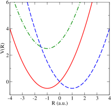
We construct a series of four models, three of which are symmetric and differ only in the strength of the nonadiabatic coupling. The fourth model is an asymmetric system where one diabatic state is significantly higher in energy than the other. All simulations are performed at a temperature $\beta=1$ a.u., with nuclear mass $M=1$ a.u. and potential parameters $k=a=1$ a.u. The coupling strength and asymmetry for each model are provided in Table 1. The potential energy curves for the symmetric and asymmetric models are shown in Fig. 1.

Figure 1: The diagonal elements of the potential energy matrix, $V_{nn}(R)+V_{0}(R)$, are shown in red (solid line) for electronic state 1 and in blue (dashed line) for electronic state 2. The green curve (dot-dashed line) corresponds to electronic state 1 for the asymmetric model.

Model	$c$	$\Delta$
I	0.0	0.10
II	0.0	1.00
III	0.0	10.0
IV	3.0	0.10

Table 1: Parameters for Models I-IV. All parameters are specified in atomic units.

We calculate the nuclear position TCFs for all four model systems. The MV-RPMD results are obtained by evaluating Eq. (38). The initial distribution in electronic and nuclear positions and momenta for all simulations is sampled using PIMC, and a total of $10^{5}$ points are generated for each model system. MV-RPMD trajectories are initialized from this initial distribution and the equations of motion are integrated for $20$ a.u. using a $4^{\text{th}}$ order Adams-Bashforth-Moulton predictor-corrector integrator. The initial distribution in the MF-RPMD simulations are sampled using PIMC, and a total of $10^{3}$ points are generated for each model system. Trajectories initialized from this distribution are time evolved for $20$ a.u., and the TCFs are calculated using Eq. (II.4). We report convergence parameters for both MV-RPMD and MF-RPMD simulations in Table 2 for all four model systems. The Kubo-transformed TCF in Eq. (36) for each model is obtained from a numerically exact discrete-variable representation (DVR) grid calculation. dtc92

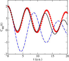
Model I lies in the weak-coupling regime where $\Delta~{}<<~{}kT$. This is the most physically relevant regime for nonadiabatic electron transfer, proton-coupled electron transfer and exciton dynamics, and it is also where the mean-field approximation breaks down. In Fig. 2, we compare the TCFs obtained from MV-RPMD and MF-RPMD simulations with the exact quantum result. While both simulations are exact at time zero, the MF approximation does not hold in this regime, and even at very short times the TCF is dramatically different from the exact result. In contrast, MV-RPMD performs remarkably well: the TCF is identical to the quantum result at short times and starts to deviate only at longer times.

Figure 2: The nuclear position-position TCF for Model I obtained using MV-RPMD is shown in red (solid line with squares), the TCF using MF-RPMD is shown in blue (dashed line), and the exact DVR grid calculation is shown in black (solid line).

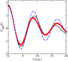
Model II describes a symmetric two-level system with intermediate coupling strength, $\Delta~{}\approx~{}kT$. The nuclear position TCFs for this model are shown in Fig. 3. The MF-RPMD result is much improved for this model and correctly captures the timescales of oscillation in the nuclear positions. MV-RPMD outperforms MF-RPMD again in this regime, being nearly identical at short times and deviating slightly at longer times from the exact result.

Figure 3: The nuclear position-position TCF for Model II obtained using MV-RPMD is shown in red (solid line with squares), the TCF using MF-RPMD is shown in blue (dashed line), and the exact DVR grid calculation is shown in black (solid line).

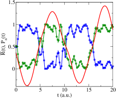
To confirm that the MV-RPMD trajectories preserve the Boltzmann distribution, we calculate averages over the ensemble of trajectories used in the $P=5$ bead simulation for Model II. The average nuclear center-of-mass coordinate and electronic state populations are found to stay constant as a function of time for the length of our simulation, as expected. We demonstrate the potential utility of MV-RPMD for direct dynamics by calculating instantaneous values of electronic state populations from Eq. (39) and nuclear center-of-mass coordinate along a single, representative trajectory. In Fig. 4 we show that for this intermediate coupling regime electronic state populations oscillate on the timescale of the nuclear vibrational motion.

Figure 4: The instantaneous values of electronic state populations for Model II are shown in blue (with squares) for state 1 and in green (with circles) for state 2, and the nuclear center-of-mass coordinate is shown in red (solid line) along a single MV-RPMD trajectory. The nuclear coordinate is scaled and shifted such that the diabatic potentials appear to cross at $R=0.5$ rather than $R=0$ for clarity.

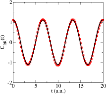
Model III represents the strong coupling regime where $\Delta~{}>>~{}kT$. The mean-field approximation works well in this regime; the results from our simulation were identical to the exact quantum result and are not shown here. In Fig. 5, we compare the MV-RPMD correlation function with the exact quantum results, and find that it is nearly identical at all times.

Figure 5: The nuclear position-position TCF for Model III obtained using MV-RPMD is shown in red (solid line with squares) and the exact DVR grid calculation is shown in black (solid line). The MF-RPMD TCF is not plotted, as it is also nearly identical with the exact quantum TCF.

Model	MV-RPMD		MF-RPMD
	$P$	$N_{\text{T}}$	$P$	$N_{\text{T}}$
I	4	5000	4	1000
II	5	8000	5	1000
III	10	20000	10	2000
IV	5	8000	5	1000

Table 2: Convergence parameters for MF-RPMD and MV-RPMD calculations of the nuclear TCFs for Models I-IV. We report the number of path beads, $P$, and the number of trajectories, $N_{\text{T}}$, used for each simulation.

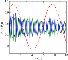
In Fig. 6, we present the instantaneous values of electronic state populations and nuclear center-of-mass coordinate for Model III along a representative trajectory. In this strong coupling regime, we observe the clear separation between the fast timescales on which electronic state populations oscillate about the equilibrium value of $0.5$ and the slower timescale associated with nuclear vibrational motion. Comparing Fig. 4 with Fig. 6 we observe the change in mechanism from a regime where nonadiabatic transitions between electronic states are coupled to nuclear vibrations to the mean-field regime where nuclear motion occurs on an average electronic potential surface.

Figure 6: The instantaneous values of the electronic state populations for Model III are shown in blue (solid line) for state 1 and in green (solid line) for state 2, and the nuclear center-of-mass coordinate is shown in red (dashed line) along a single MV-RPMD trajectory. The nuclear coordinate is scaled and shifted such that the diabatic potentials appear to cross at $R=0.5$ rather than $R=0$, and we only show the first $10$ a.u. of the trajectory for clarity.

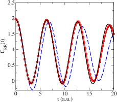
Our asymmetric system, Model IV, has potential energy diabats as shown in Fig. 1 and is in the weak-coupling regime. The system is deliberately chosen to resemble the inverted regime in a system-bath model for electron transfer, a case known to challenge the accuracy of the position-space, nonadiabatic RPMD approacharm11 . In Fig. 7 we show the remarkable agreement between the MV-RPMD TCF and the exact quantum result. MF-RPMD performs reasonably well, but agrees with the exact results only at very short times and fails to capture the correct timescale for nuclear motion.

Figure 7: The nuclear position-position TCFs for Model IV obtained using MV-RPMD is shown in red (solid line with squares), the TCF using MF-RPMD is shown in blue (dashed line), and the exact DVR grid calculation is shown in black (solid line).

The number of trajectories, $N_{\text{T}}$, required to converge the TCF calculations for all four models described here are recorded in Table 2. We note that although the computational expense is comparable to a low-cost linearized semiclassical implementation,na10 the resulting TCFs are expected to be numerically more accurate since MV-RPMD avoids the problem of zero-point energy leakage by employing trajectories that preserve the QBD. Further, we find the sign function, $\text{sgn}(\Theta)$, in the Eq. (38) does not give rise to a numerical sign problem in the calculations presented here, which we attribute to the non-oscillatory structure of the QBD from which our dynamics is derived. We also report the number of path-beads, $P$, required to converge the TCF calculations in Table 2. The validity of the short-time approximation for the electronic state matrix elements in Eq. (10) is related to the coupling strength, as evidenced by an increase in the number of path-beads required as we go from the weak-coupling to the strong-coupling regime. The MV-RPMD approach is thus particularly suited for simulating chemistry in the weak-coupling limit. It is notable that the MV-RPMD method is able to accurately describe nonadiabatic dynamics over a wide range of coupling strengths and also correctly describes asymmetric tunneling.

Looking forward, for the calculation of chemical reaction rates in general nonadiabatic systems, it will be desirable to identify good order parameters in the electronic state variables as well as in nuclear coordinates. In addition, while the MV-RPMD method is very promising for applications to photochemical processes, the fundamental success of RPMD in describing quantum dynamics, despite recent progress, sh13 ; tjhh13 is not fully understoond and requires further theoretical investigation.

IV Conclusion

In this paper we derive a novel imaginary-time PI based dynamics, MV-RPMD, that extends the applicability of RPMD to multi-electron processes. Using standard benchmark models for nonadiabatic systems, we demonstrate that the MV-RPMD dynamics are capable of accurately simulating TCFs for model systems with coupling strengths that range over two orders of magnitude. We also demonstrate that the method is robust to asymmetries in the diabatic electronic states.

We expect this model dynamics to open the door to large-scale simulations of photo-induced charge and energy transfer in the condensed phase. Future applications include exciton dynamics in photovoltaic materials as well as mechanistic studies of multi-electron transfer reactions in transition-metal catalysts.

V Acknowledgements

The author sincerely thanks T. F. Miller III for several valuable discussions. This work was supported by a start-up grant from Cornell University.

VI Appendix: Wigner transform of the electronic integral

We start with Eq. (23) for the electronic integral,

$$I_{E}=\frac{1}{(2\pi\hbar)^{PN}}\int d\{\mathbf{x}_{\alpha}\}\int d\{\mathbf{p}_{\alpha}\}\int d\{\Delta\mathbf{x}_{\alpha}\}$$

$$\;\;\prod_{\alpha=1}^{P}\langle\mathbf{x}_{\alpha}-\frac{\Delta\mathbf{x}_{\alpha}}{2}|\mathcal{P}e^{\beta_{P}\mathbf{V}(\mathbf{R}_{\alpha})}\mathcal{P}|\mathbf{x}_{\alpha+1}+\frac{\Delta\mathbf{x}_{\alpha+1}}{2}\rangle\;e^{i\mathbf{p}_{\alpha}^{T}\cdot\Delta\mathbf{x}_{\alpha}},$$

and substitute Eq. (9) and Eq. (10) to obtain

$$I_{E} = \frac{1}{(2\pi\hbar)^{PN}}\int d\{\mathbf{x}_{\alpha}\}\int d\{\mathbf{p}_{\alpha}\}\int d\{\Delta\mathbf{x}_{\alpha}\}$$ (49)

$$\times \prod_{\alpha=1}^{P}\left(\mathbf{x}_{\alpha}-\frac{\Delta\mathbf{x}_{\alpha}}{2}\right)^{T}\cdot\mathbf{\mathcal{M}}(\mathbf{R}_{\alpha})\cdot\left(\mathbf{x}_{\alpha+1}+\frac{\Delta\mathbf{x}_{\alpha+1}}{2}\right)$$

$$\times e^{-\sum_{\alpha=1}^{P}\left(\frac{1}{4}\Delta\mathbf{x}_{\alpha}^{T}\cdot\Delta\mathbf{x}_{\alpha}+\mathbf{x}_{\alpha}^{T}\cdot\mathbf{x}_{\alpha}+\mathbf{p}_{\alpha}^{T}\cdot\mathbf{p}_{\alpha}-i\mathbf{p}_{\alpha}^{T}\cdot\Delta\mathbf{x}_{\alpha}\right)}.$$

The pre-exponential function in Eq. (49) can be re-arranged to group like terms in $\{\Delta\mathbf{x}_{\alpha}\}$,

$$I_{E} = \frac{1}{(2\pi\hbar)^{PN}}\int d\{\mathbf{x}_{\alpha}\}\int d\{\mathbf{p}_{\alpha}\}\int d\{\Delta\mathbf{x}_{\alpha}\}$$ (50)

$$\times \text{Tr}\left[\prod_{\alpha=1}^{P}\left(\mathbf{x}_{\alpha}+\frac{\Delta\mathbf{x}_{\alpha}}{2}\right)\otimes\left(\mathbf{x}_{\alpha}-\frac{\Delta\mathbf{x}_{\alpha}}{2}\right)^{T}\mathbf{\mathcal{M}}(\mathbf{R}_{\alpha})\right]$$

$$\times e^{-\sum_{\alpha=1}^{P}-\left(\frac{1}{4}\Delta\mathbf{x}_{\alpha}^{T}\cdot\Delta\mathbf{x}_{\alpha}+\mathbf{x}_{\alpha}^{T}\cdot\mathbf{x}_{\alpha}+\mathbf{p}_{\alpha}^{T}\cdot\mathbf{p}_{\alpha}-i\mathbf{p}_{\alpha}^{T}\cdot\Delta\mathbf{x}_{\alpha}\right)}.$$

The resulting integral over $\{\Delta\mathbf{x}_{\alpha}\}$ is of Gaussian form and can be analytically evaluated to obtain Eq. (24).

References

• (1) J. L. Bredas, D. Beljonne, V. Coropceanu, and J. Cornil, Chem. Rev. 104, 4971 (2004).
• (2) M. B. Smith and J. Michl, Chem. Rev. 110, 6891 (2010).
• (3) M. Mickler, E. Schleiff, and T. Hugel, Chem. Phys. Chem. 9, 1503 (2008).
• (4) P. Ceroni, A. Credi, M. Venturi, and V. Balzani, Photochem. Photobiol. Sci. 9, 1561 (2010).
• (5) R. I. Cukier and D. G. Nocera, Ann. Rev. Phys. Chem. 49, 337 (1998).
• (6) J. L. Dempsey, A. J. Esswein, D. R. Manke, J. Rosenthal, J. D. Soper, and D. G. Nocera, Inorg. Chem. 44, 6879 (2005).
• (7) E. Rabani, S. A. Egorov, and B. J. Berne, J. Phys. Chem. A 103, 9539 (1999).
• (8) J. C. Burant and J. C. Tully, J. Chem. Phys. 112, 6097 (2000).
• (9) W. H. Miller, J. Phys. Chem. A 113, 1405 (2009).
• (10) J. Caro and L. L. Salcedo, Phys. Rev. A 60, 842 (1999).
• (11) P. Ehrenfest, Z. Phys. 45, 455 (1927).
• (12) C. Zhu, A. W. Jasper, and D. G. Truhlar, J. Chem. Phys. 120, 5543 (2004).
• (13) P. Pechukas, Phys. Rev. 181, 166 (1969).
• (14) R. Kapral and G. Ciccotti, J. Chem. Phys. 110, 8919 (1999).
• (15) A. Donoso and C. C. Martens, J. Chem. Phys. 112, 3980 (2000).
• (16) J. C. Tully, J. Chem. Phys. 93, 1061 (1990).
• (17) O. V. Prezhdo, and P. J. Rossky, J. Chem. Phys. 107, 825 (1997).
• (18) A. W. Jasper, S. N. Stechmann, and D. G. Truhlar, J. Chem. Phys. 116, 5424 (2002).
• (19) M. F. Herman, J. Chem. Phys. 103, 8081 (1995).
• (20) Y. H. Wu and M. F. Herman, J. Chem. Phys. 127, 044109 (2007).
• (21) J. C. Tully, Ann. Rev. Phys. Chem. 51, 153 (2000).
• (22) A. Kelly, R. van Zon, J. Schofield, and R. Kapral, J. Chem. Phys. 136, 084101 (2012).
• (23) C. D. Schwieters and G. A. Voth, J. Chem. Phys. 111, 2869 (1999).
• (24) J. L. Liao, and G. A. Voth, J. Phys. Chem. B 106, 8449 (2002).
• (25) X. Sun and W. H. Miller, J. Chem. Phys. 106, 6346 (1997).
• (26) N.Ananth, C. Venkataraman and W. H. Miller, J. Chem. Phys. 127, 084114 (2007).
• (27) S. Bonella and D. F. Coker, J. Chem. Phys. 122, 194102 (2005).
• (28) P. Huo and D. F. Coker, J. Chem. Phys. 133, 184108 (2010).
• (29) I. R. Craig and D. E. Manolopoulos, J. Chem. Phys. 121, 3368 (2004).
• (30) S. Habershon, D. E. Manolopoulos, T. E. Markland, and T. F. Miller, III, Ann. Rev. Phys. Chem. 64, 387 (2013).
• (31) T. F. Miller III and D. E. Manolopoulos, J. Chem. Phys., 122, 184503 (2005).
• (32) T. E. Markland, S. Habershon and D. E. Manolopoulos, J. Chem. Phys. 128, 194506 (2008).
• (33) S. Habershon, T. E. Markland and D. E. Manolopoulos, J. Chem. Phys. 131, 024501 (2009).
• (34) N. Boekelheide, R. Salomón-Ferrer, and T. F. Miller III, Proc. Nat. Acad. Sci. USA, 108, 16159 (2011).
• (35) T. F. Miller III, J. Chem. Phys., 129, 194502 (2008).
• (36) A. R. Menzeleev and T. F. Miller III, J. Chem. Phys., 132, 034106 (2010).
• (37) A. R. Menzeleev, N. Ananth, and T. F. Miller III, J. Chem. Phys., 135, 074106 (2011).
• (38) J. S. Kretchmer and T. F. Miller III, J. Chem. Phys., 138, 134109 (2013).
• (39) N. Ananth and T. F. Miller III, J. Chem. Phys., 133, 234103 (2010).
• (40) H. D. Meyer, and W. H. Miller, J. Chem. Phys. 70, 3214 (1979).
• (41) G. Stock, and M. Thoss, Phys. Rev. Lett. 78, 578 (1997).
• (42) H. F. Trotter, Proc. Amer. Math. Soc. 10, 545 (1958).
• (43) D. Chandler, Introduction to Modern Statistical Mechanics, pg. 149 (Oxford University Press, New York, 1987).
• (44) M. Parrinello and A. Rahman, J. Chem. Phys. 80, 860 (1984).
• (45) H. Weyl, Z. Phys. 46, 1 (1927).
• (46) E. Wigner, Phys. Rev. 40, 79 (1932).
• (47) E. Wigner, Z. Phys. Chem. B19, 203 (1932).
• (48) J. E. Moyal, Math. Proc. Cambridge Philos. Soc. 45, 99 (1949).
• (49) The mean-field RPMD approximation is not a new idea, and has been used previously to benchmark nonadiabatic PI methods by D. E. Manolopoulos, T. F. Miller, III, J. C. Tully and I. R. Craig.
• (50) D. T. Colbert, and W. H. Miller, J. Chem. Phys. 96, 1982 (1992).
• (51) T. J. H. Hele and S. C. Althorpe, J. Chem. Phys. 138, 084108 (2013).