SATMC: Spectral Energy Distribution Analysis Through Markov Chains

Abstract

We present the general purpose spectral energy distribution (SED) fitting tool SED Analysis Through Markov Chains (SATMC). Utilizing Monte Carlo Markov Chain (MCMC) algorithms, SATMC fits an observed SED to SED templates or models of the user’s choice to infer intrinsic parameters, generate confidence levels and produce the posterior parameter distribution. Here we describe the key features of SATMC from the underlying MCMC engine to specific features for handling SED fitting. We detail several test cases of SATMC, comparing results obtained to traditional least-squares methods, which highlight its accuracy, robustness and wide range of possible applications. We also present a sample of submillimetre galaxies that have been fitted using the SED synthesis routine GRASIL as input. In general, these SMGs are shown to occupy a large volume of parameter space, particularly in regards to their star formation rates which range from $\sim$30-3000 M_⊙ yr^-1 and stellar masses which range from $\sim 10^{10}-10^{12}$ M_⊙. Taking advantage of the Bayesian formalism inherent to SATMC, we also show how the fitting results may change under different parametrizations (i.e., different initial mass functions) and through additional or improved photometry, the latter being crucial to the study of high-redshift galaxies.

1 Introduction

The complete pan-chromatic spectral energy distribution (SED) of a source encodes a wealth of information concerning its age, mass, metallicity, dust/gas content, star formation rate (SFR), star formation history (SFH) and more. Various emission mechanisms account for the apparent shape and typical features found in SEDs. For example, dust reprocessing results in attenuation of optical/ultra-violet (UV) photons produced from stellar populations whose energy is then re-emitted at infrared (IR) wavelengths while specific species of ions and molecules produce emission/absorption features across the electromagnetic spectrum. Unfortunately, our ability to extract information from observations is hampered both on the observational and theoretical sides. As observers, we try to make due with either coarse, broad-band sampling of a source’s SED or with high resolution sampling of a small portion of the SED through spectroscopy. Theorists, on the other hand, must make difficult decisions regarding which physics, spatial scales, and evolutionary histories to include in the creation of their SED libraries or synthesis models.

Within the literature, SED models can be sub-categorized into two main types. Empirical models are derived for particular classifications based on a subset of similar sources (e.g. Arp 220 and M82 for starburst galaxies, the quasar mean template, etc.). These models offer the simplest approximation of a source’s SED and are generally preferred when only sparse photometry is available or for coarse estimates of basic properties (e.g. luminosity, SFR, colors). The underlying assumption behind empirical models, namely that all sources of that ’type’ have the same SED, is difficult to verify and so their use to probe all but the grossest properties is limited.

Theoretical models are constructed from sets of physical and radiative processes believed to be the dominant contributors to the emission of a source. Functionally, these again are divided into two classes. Pre-computed template libraries for particular source types are the most widely used (e.g. Calzetti et al., 2000; Efstatiou, Rowan-Robinson & Siebenmorgen, 2000; Siebenmorgen et al., 2004; Siebenmorgen & Krügel, 2007; Gawiser, 2009; Michalowski, Watson & Hjorth, 2010, and references therein). Since they are pre-computed, these libraries allow the rapid exploration of a pre-defined parameter space at the expense of being limited to the resolution and scope of the parameter space provided by the authors. For more generalized applications, SED synthesis packages are now available that offer a wider set of input parameters and the exploration of a continuous parameter space (e.g. stellar population synthesis codes such as GALAXEV, Bruzual & Charlot (2003) and pan-chromatic galaxy synthesis codes like GRASIL, Silva et al. (1998) and CIGALE, Noll et al. (2009)). Of course, one may use these packages to construct ones own template libraries (e.g. Michalowski, Watson & Hjorth, 2010) for specific applications as well. In both cases, as the generality of the underlying physics increases to provide relevance to a wider class of sources, so does the number of free parameters in the models. The unavoidable existence of correlations in these parameters insists that simply finding a best-fit parametrization is no longer sufficient. Rather, we now require tools that properly reveal the complexities and correlations in the adopted model parameter space.

With this in mind, here we present the general purpose MCMC-based SED fitting code SED Analysis Through Markov Chains or SATMC. Monte Carlo Markov Chain (MCMC) techniques are a set of methods based in the Bayesian formalism which enable efficient sampling of multi-dimensional parameter spaces in order to construct a distribution proportional to the probability density distribution of the input parameters, known as the posterior parameter distribution or simply the posterior. The posterior identifies the nuances in parameter space, including any possible correlations, making MCMCs particularly useful for exploring SED models and libraries with high dimensionality. MCMC based SED fitting codes are relatively new but have been growing in popularity (e.g. Sajina et al., 2006; Acquaviva, Gawiser & Guaita, 2011; Serra et al., 2011; Pirzkal et al., 2012). In addition to deriving the posterior for best fit parameter and confidence level estimation, SATMC includes many features to aid in improving performance and allows users to easily incorporate additional knowledge and constraints on parameter space in the form of priors. Additionally, SATMC versions exist in both IDL and Python and both are modular and straightforward to use in any wavelength regime and for any class of sources.

This paper is organized as follows. We start by detailing the MCMC algorithm and the basic process for MCMC-based SED fitting. We then provide case examples displaying the versatility and accuracy of SATMC compared to standard least-squares methods. As part of this demonstration, we also present a set of SEDs derived from SATMC when used in conjunction with the SED synthesis routine GRASIL to a sample of X-ray selected starburst galaxies. These fits highlight the key advantages obtained from the MCMC-based approach and their agreement with similar classes of composite SEDs.

2 SATMC: The MCMC Algorithm

The primary motivation for SATMC is to provide a means for efficient sampling of a parameter space with $n_{D}$ free parameters in order to derive parameter estimates and their associated confidence intervals. This is accomplished by sampling an $n_{D}$-dimensional surface proportional to the probability density function of the parameters given the data $P(\textbf{x}|\textbf{D})$, also referred to as the posterior parameter distribution. We determine the posterior through Bayes Theorem

$$P(\textbf{x}|\textbf{D})\propto P(\textbf{D}|\textbf{x})P(\textbf{x})$$ (1)

where $P(\textbf{x})$ represents our current knowledge of the parameters or priors and $P(\textbf{D}|\textbf{x})$ is the probability of the data given the model parameters, often referred to as the likelihood $L$. We shall define the general form of the likelihood according to

$$P(\textbf{D}|\textbf{x})=L=\prod^{M}_{i-1}{\rm exp}(\frac{(D_{i}-f(d_{i}|\textbf{x}))^{2}}{2\sigma^{2}_{i}})$$ (2)

where the product runs over the M observed data points ${\bf D}$ whose individual variances are given by $\sigma_{i}^{2}$ and the function $f({\bf d}|{\bf x})$ represents the model observations ${\bf d}$ for the set of ${\bf x}$ parameters. Note, however, that this prescription of $L$ assumes that the observations have Gaussian distributed errors, an assumption we will return to later in § 3.1. In the following sections, we detail specific MCMC features that define the basic operation of SATMC.

2.1 MCMC Acceptance and Convergence

Within the literature, there are a variety of sampling algorithms one may use to construct an MCMC (e.g. Metropolis-Hastings or Gibbs sampling; Metroplois et al., 1953; Hastings, 1970; Geman & Geman, 1984; Geyer, 1992; Chib & Jeliazkov, 2001; Verde et al., 2003; Mackay, 2003). For SATMC, we employ the Metropolis-Hastings algorithm which works as follows:

• Generate a proposal distribution $q({\bf x_{i}|x_{i-1}})$ from which the candidate steps ${\bf x_{i}}$ will be drawn

• Calculate the acceptance probability according to the likelihood ratio ($\alpha=$min(1,$\frac{P({\bf x_{i}}|{\bf D})q({\bf x_{i}|x_{i-1}})}{P({\bf x_{i-1}}|{\bf D})q({\bf x_{i-1}|x_{i}})}$))

• Draw a uniformly distributed random number $u$ from 0 to 1 and accept the step if $u<\alpha$, reject otherwise

• Repeat for the next step

Though the exact choice of $q({\bf x_{i}|x_{i-1}})$ is arbitrary, it is common to adopt an $n_{D}$-dimensional multivariate-Normal distribution $\mathcal{N}$(${\bf\mu},\Sigma$) with $\Sigma=\sigma_{\bf x}^{2}$I where I is the identity matrix, $\sigma_{\bf x}$ is the variance of each parameter in x and

$$\mathcal{N}({\bf\mu},\Sigma)\propto|\Sigma|^{-\frac{1}{2}}{\rm e}^{-\frac{1}{2}({\bf x}-{\bf\mu})^{\prime}\Sigma^{-1}({\bf x}-{\bf\mu})}$$ (3)

for generating proposed steps (e.g. Gelman, Roberts & Gilks, 1995; Roberts, Gelman, & Gilks, 1997; Roberts & Rosenthal, 2001; Atchade & Rosenthal, 2005). Following these works, it is found that the distribution $\mathcal{N}$(${\bf\mu},\Sigma$) should be tuned for optimal performance between the time necessary to reach a stable solution (referred to as the burn-in period) and sampling of the posterior, which may be achieved by adjusting $\mathcal{N}$(${\bf\mu},\Sigma$) until the resulting chains have acceptance rates of $\sim$23 percent in the limit of large dimensionality. We therefore base our proposal distribution around an adaptive covariance matrix $\Sigma$ (similar to Acquaviva, Gawiser & Guaita, 2011) such that samples are drawn from the multivariate-Normal distribution now given by $\mathcal{N}$(${\bf x_{i-1}},\Sigma$). To obtain an acceptance rate of $\sim$23 percent, we start by initializing the covariance matrix for each chain as $\sigma_{\bf x}^{2}$I where $\sigma_{\bf x}$ is set proportional to the input parameter ranges. After a period of steps, we then calculate $\Sigma$ directly from the chain over the previous interval, i.e.

$$\Sigma={\rm E}[({\bf x}-{\rm E}[{\bf x}])({\bf x}-{\rm E}({\bf x}))^{T}]$$ (4)

where $E[{\bf x}]$ is the expectation value or weighted average of ${\bf x}$. Following each period of steps, we compute the acceptance rate and scale $\Sigma$ if the acceptance rate is too high ($>$26 percent) or too low ($<$20 percent). The covariance matrix is continuously updated until the target $\sim$23 percent acceptance is reached, which allows $\Sigma$ to take on the shape of the underlying posterior to readily identify and account for possible correlations in the parameters.

Once the target acceptance rate has been reached, we then check for chain convergence to determine when the burn-in period is complete. In the MCMC literature there are many approaches to determine convergence (e.g. Gelman & Rubin, 1992; Gilks, Richardson & Spiegelhalter, 1996; Raftery & Lewis, 1992); we opt for the Geweke diagnostic (Geweke, 1992) which compares the average and variance of samples obtained in the first 10 percent and last 50 percent of a chain segment. If the two averages are equal (within the tolerance set by their variances), then the chain is deemed to be stationary and convergence is complete. We check both the acceptance rate and convergence, verifying the acceptance rate before checking for convergence, over a default period of 1000 steps until both have been satisfied. If necessary, the covariance matrix is modified to maintain the target acceptance rate. Once both criteria are fulfilled, burn-in is completed and the chain(s) are set to continue to provide sampling of the posterior.

2.2 Parallel Tempering

Figure 1: Simple visualization of transitions between tempered chains. Transitions may occur either between the cold and tempered chains (top) or between adjacent pairs (bottom). The former allows for rapid sampling of parameter space to quickly reach a global maxima while the latter improves sampling around a single location to avoid local maxima in the construction the posterior parameter distribution. In this example, chain transitions are proposed after every 100 steps; in practice, these transitions are proposed every 3000 steps.

When constructing the posterior distribution, we must be careful to sample all of the nuances of parameter space as the posterior distribution is not guaranteed to be a smooth or even continuous function of the free parameters. As with all fitting approaches, the existence of local maxima in the posterior requires that either we known a priori the general location of the global maximum or we implement a sampling technique capable of increasing the probability of finding it. For example, one could choose to initialize a large number of chains that cover random locations throughout parameter space. While this approach is nearly guaranteed to find the global maximum, it is also extremely inefficient. SATMC utilizes a technique known as “Parallel Tempering” (see review by Earl & Deem, 2005) which, in analogy to simulated annealing, uses several chains – each with progressive modifications to likelihood space parametrized as a statistical ’temperature’ – to search parameter space and exchange information about the posterior at each chain’s location. For a given chain at temperature T, the likelihood is ’flattened’ according to $L_{T}=L^{1/(1+T)}$. The tempered chains thus distort likelihood space, exchanging sensitivity to the details within posterior for the general shape, such that chains with higher temperatures will accept more steps, and thus sample larger regions of parameter space. By coupling these tempered chains, we allow ’colder’ chains to access areas of parameter space they may have otherwise been unable to reach. The process for handling tempered chains works as follows:

• Temperatures are assigned to chains in a progressive manner with one chain designated the fiducial ’cold’ chain with $T=0$ (e.g. $T=[0,10,100,1000]$).

• Chains are allowed to progress for a set number of steps (SATMC uses 3 iterations of acceptance/convergence or 3000 steps by default)

• A ’swap’ of chain state information is proposed using the Metropolis acceptance algorithm $\alpha={\rm min}(1,\frac{(P({\bf x_{i}}|{\bf D}))^{1/(1+T_{j})}(P({\bf x_{j}}|{\bf D}))^{1/(1+T_{i})}}{(P({\bf x_{i}}|{\bf D}))^{1/(1+T_{i})}(P({\bf x_{j}}|{\bf D}))^{1/(1+T_{j})}}$

• The new set of chains is then allowed to run until the next swap of chain state information.

This process of coupling individual chains with a Metropolis-Hastings acceptance algorithm was initially proposed by Geyer (1991) and is referred to as a Metropolis Coupled Monte Carlo Markov Chain or MC³. When applying temperatures to individual chains, the sampling of each chain will vary due to the distortions of likelihood space; i.e., a chain at a higher temperature will accept more steps than a chain with an identical proposal distribution at lower temperature. To maintain a reasonable sampling of the tempered likelihoods, each chain is treated individually for the purposes of acceptance and convergence testing. Note, however, that updating the tempered chains occurs only with the acceptance and convergence testing of the cold chain. This ensures that we obtain a proper sampling of the posterior without being influenced by the otherwise distorted likelihood space. In parallel tempering techniques, one can specify whether the potential swaps occur only between the cold and any tempered chain (0,$j$) or between adjacent chains ($i,i\pm$1) (see Fig. 1). The former allows for rapid sampling and mixing of the chains to determine the global maximum and is thus used during the burn-in period. The latter passes state information down through the tempered chains so that the cold chain may access a more representative region of parameter space; this method is used after burn-in to properly sample parameter space around the maximum likelihood. In this case, chains progress for a set length (500 steps by default) whereafter the chain transitions are proposed. Should a swap be made with the cold chain after burn-in is complete, we re-compute the acceptance rate and convergence as outlined in the previous section to verify proper sampling. Due to the modified acceptance rate and misshapen likelihood space of the tempered chains, it is generally undesirable to use them in re-constructing the posterior parameter distribution. If there have been no swaps to the cold chain after 10 iterations, the temperatures of all chains are set to 0 and the MCMC is allowed to continue until sufficient samples of the posterior distribution around the maximum have been obtained.

3 SATMC SED Specific Features

The methods presented in § 2 are generalized for any MCMC-based algorithm. Here, we detail specific modifications and methods utilized in SATMC for SED fitting.

3.1 Observations and Upper Limits

In order to perform a fit, SATMC requires at least two sets of information: 1) a file containing the M observations including their wavelengths ($\lambda_{i}$) or frequencies ($\nu_{i}$), observed fluxes ($f_{\rm obs,i}$) and corresponding uncertainties ($\sigma_{\rm obs,i}$) and 2) the model libraries. Following from Eqn. 2, we define the likelihood for a given set of observations and models as

$$L=\displaystyle\prod^{M}_{i-1}{\rm exp}(-\frac{(f_{\rm obs,i}-f_{\rm mod,i})^{2}}{2\sigma_{f_{\rm obs,i}}^{2}})$$ (5)

or similarly

$$\ln(L)=\displaystyle\sum^{M}_{i-1}-\frac{(f_{\rm obs,i}-f_{\rm mod,i})^{2}}{2\sigma_{f_{\rm obs,i}}^{2}}$$ (6)

where $f_{\rm mod,i}$ are the model fluxes which for narrow passbands are interpolated model SED values at the observed frequency/wavelength. Alternatively, $f_{\rm mod,i}$ may be calculated from a set of passbands with a given filter response ($p(\nu)$ as provided by the user) as

$$f_{mod,i}=\frac{\int_{\nu_{min}}^{\nu_{max}}{\rm SED}(\nu)p_{i}(\nu){\rm~{}d}\nu}{\int_{\nu_{min}}^{\nu_{max}}p_{i}(\nu){\rm~{}d}\nu}$$ (7)

where $\nu_{min}$ and $\nu_{max}$ are taken from the filter files.

Figure 2: Example likelihood distribution for upper limits. Here, the upper limit has a value of 3 mJy (dotted vertical line). The remaining lines represent the likelihood distribution for the simple step function (solid), one-sided Gaussians assuming the upper limit is at the 5$\sigma$ level with a cut-off at 1.8 mJy (dashed) and 0 mJy (dot-dash) and one-sided Gaussians with the upper limit at the 3$\sigma$ level and cut-offs at 2 mJy (triple dot-dash) and 0 (long dash).

In cases where there is no detection but only an upper limit, SATMC provides a parametrized probability distribution to allow the user to reflect their confidence in the underlying statistics of the observations. A simple approach for incorporating upper limits is to assume a step function accepting all models that fall below the limit and rejecting all that lie above. While attractive in its simplicity, this method harshly truncates regions of parameter space and improperly weights the upper limit’s contribution to $L$. To partially alleviate these issues, SATMC implements a one-sided Gaussian distribution so that models with fluxes above the upper limit may contribute to the posterior with a small but non-zero probability (see also Feigelson & Nelson, 1985; Isobe, Feigelson & Nelson, 1986; Sawicki, 2012). The one-sided Gaussian is defined by

$$L^{\prime}\propto\left\{\begin{array}[]{cl}1&\mbox{ if $f_{mod}<f_{\rm co}$}\\ {\rm exp}(-\frac{(f_{\rm co}-f_{mod})^{2}}{2\sigma_{\rm co}^{2}})&\mbox{ if $f_{mod}\geq f_{\rm co}$}\end{array}\right.$$ (8)

where $f_{\rm co}$ represents the cut-off transition from flat $L^{\prime}$=1 to a Gaussian ’tail’ with standard deviation $\sigma_{co}$. Parametrizing the probability distribution in this manner allows for a compromise between the simple step function, also available in SATMC, and over-interpreting the shape of the noise distribution at small fluxes, as demonstrated in Fig. 2.

3.2 Photometric Redshift Estimation

Since redshift is just another parameter in a source’s SED, SATMC is capable of providing photometric redshift (photo-z) determinations for sources in the context of the input SED models. Traditionally, photo-z codes implement least-squares methods (e.g. HYPERZ Bolzonella, Miralles & Pelló, 2000) though some recent codes have adopted the Bayesian formalism for using priors (e.g. BPZ, Benitez 2000; EAZY, Brammer, van Dokkum & Coppi (2008)).

The standard approach in photo-z estimation is to apply an SED library (often limited to a few galaxy types) to find the photo-z and then repeat the fitting using the same (or in some cases different) library fixed at the photo-z to estimate source properties. This approach under-estimates the true errors on the photo-z and other fitted parameters. SATMC fits the redshift simultaneously with all other parameters and produces a direct determination of the redshift-parameter probability distributions in addition to the marginalized redshift probability distribution $P(z)$.

We have tested and improved the photo-z estimation with SATMC in collaboration with the CANDELS team. Dahlen et al. (2013) provides a complete analysis of various photometric redshift estimation techniques for samples of CANDLES galaxies in the GOODS-S field (Giavalisco et al., 2004). Out of the 13 participating groups, SATMC was the only MCMC-based code used to generate photo-z’s. Since the tests reported in Dahlen et al., we have reduced the outlier fraction (fraction of sources with $(z_{spec}-z_{phot})/(1+z_{spec})>0.15$) from $\sim$9-14 percent to $\sim$3-8 percent through modification of our input templates, luminosity priors (e.g. Kodama, Bell & Bower, 1999; Benitez, 2000) and zero-point photometry corrections (e.g. Dahlen et al., 2010).

3.3 Template Libraries and SED Synthesis Routines

As MCMC samplers require a continuous parameter space, SATMC allows the user to incorporate SED synthesis routines (e.g. GALAXEV, GRASIL, CIGALE) to generate SEDs at candidate steps and compute the resulting likelihoods. Empirical templates are often defined with a scalable normalization factor as one of the few (if any) free parameters which remains continuous when used with SATMC. Template libraries, unfortunately, rarely offer a fully continuous parameter space; often mixing sets of continuous (e.g. model normalization) and discretely sampled parameters. To create a pseudo-continuous space from such template libraries, SATMC computes the likelihoods of models bracketing the current step according to Eqns. 5 & 8 and applies multi-linear interpolation to determine the likelihood of the current proposed step. We emphasize that SATMC may be used for any class of SED models (empirical, template library or synthesis routine), so long as the appropriate interface is constructed by the user. One should note, however, that there is a trade-off between the discretely sampled template libraries or empirical templates and continuous parameter space offered by SED synthesis routines (see also Acquaviva, Gawiser & Guaita, 2011, 2012) since the run-time of the SED synthesis routines will dominate the MCMC calculation (e.g. 3+ days run-time with GRASIL versus 3-5 minutes with a template library).

Regardless of which class of SED models one wishes to adopt, empirical and theoretical SED models are commonly derived for a particular physical process and/or over a particular wavelength regime (e.g. Bruzual & Charlot, 1993; Efstatiou, Rowan-Robinson & Siebenmorgen, 2000; Siebenmorgen et al., 2004). To fully reproduce a galaxy’s SED, additional components may be required either to complete the wavelength coverage or to include a missing physical process (e.g. adding AGN emission to a star-formation template set). SATMC will construct a linear combination of multiple input SED models under the assumption that the underlying physical processes are independent. The MCMC process itself does not change: the combination of two models with $N1$ and $N2$ free parameters, respectively, is viewed as a single model with $N1+N2$ parameters when calculating likelihoods and taking potential steps.

3.4 Inclusion of Priors

An added feature of SATMC is the ability to include additional information to provide additional weights and constraints to likelihood space. In the Bayesian formalism, this extra information forms the priors of Eqn 1. For our implementation, we expand the definition of priors from the traditional Bayesian definition to include options for limiting and inherently correlating parameter space. This was deemed necessary for circumstances of fitting multiple template libraries where parameters from each model have the same physical interpretation and thus are not independent (e.g. A_V from one model library and optical depth in another) and cases where additional information not available to the fits is available (e.g. restricting the age of a galaxy at a given redshift).

3.5 Application of the Posterior

A final feature of SATMC lies in the determination of the posterior parameter distribution. As we store the likelihood and location in parameter space for each step, it becomes a simple task to construct parameter confidence intervals and even parameter-parameter confidence contours to examine relative parameter degeneracies (see Figure 3). Unfortunately, in order to visualize an $n_{D}$-dimensional parameter space, we must project or ’marginalize’ parameter space into a one or two dimensional form. When marginalizing sets of parameters, the true shape of the posterior will be distorted which may not reveal correlations in higher dimensions. This also leads to a simplification when reporting the confidence intervals on individual parameters as traditional terms such as ’1$\sigma$’ imply Gaussianity in the posterior which is unlikely to exist. Instead, one dimensional confidence levels are produced from the parameter range where 68 percent of all accepted steps are contained, marginalized over all other free parameters. Throughout the text, ’errors’ quoted when derived from SATMC refer to these marginalized parameter ranges.

4 Testing of the MCMC Algorithm

Table 1: Comparison of best-fit Siebenmorgen & Krügel 2007 parameters using standard techniques (SK07) and SATMC. For M82, we add an unreddened blackbody of temperature $T=2500$ K to the SK07 library for consistency. Note also that SK07 suggest two models for Arp220, one with $R=1$ and $A_{V}=120$ and another with $R=3$ and $A_{V}=72$ (the latter being the accepted best-fit template), which are represented in our fitting through the large uncertainties in $R$ and $A_{V}$. For each model, we also report the log-likelihood (ln(L)) of the fit. Errors are estimated at the 68 percent confidence level.

Name	SK07					SATMC
	$L_{tot}$	$R$	$A_{V}$	$L_{OB}/L_{tot}$	$n$	$L_{tot}$	$R$	$A_{V}$	$L_{OB}/L_{tot}$	$n$	ln(L)
M82	1010.5	0.35	36	0.4	10000	10${}^{10.5^{+0.2}_{-0.1}}$	0.38${}^{+0.57}_{-0.03}$	35.2${}^{+33.9}_{-14.8}$	0.418${}^{+0.167}_{-0.018}$	9710${}^{+290}_{-3907}$	-1218.7
Arp 220	1012.1	3	72	0.4	10000	10${}^{12.1^{+0.1}_{-0.2}}$	2.84${}^{+0.16}_{-1.70}$	70.1${}^{+69.5}_{-32.2}$	0.410${}^{+0.176}_{-0.010}$	190${}^{+6883}_{-90}$	-132.4

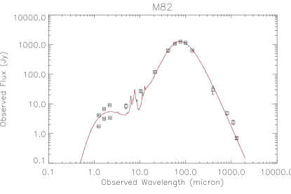
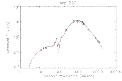
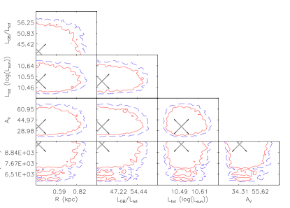
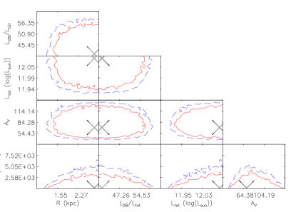
With the SATMC algorithm as outlined in § 2 and 3, we now set out to verify the fitting results by analyzing sets of well known sources and template libraries. Though the examples provided here are for galaxy SED modeling, SATMC makes no distinction between source types and may just as easily be applied to Galactic sources, localized regions within a particular galaxy or spectroscopy of individual sources. We begin with the well known galaxies Arp 220 and M82 and the starburst SED library of Siebenmorgen & Krügel (2007) (hereafter SK07) which has already been shown to provide reasonable fits to Arp 220 and M82. The SED library consists of over 7000 templates with emission from a starburst parametrized by its total luminosity $L^{tot}$, nuclear radius $R$, visual extinction $A_{V}$, ratio of luminosity from OB stars to the total luminosity and hot spot dust density $n$. The observed SEDs for Arp220 and M82 were constructed from data available on the NASA/IPAC Extragalactic Database (NED) over the 1-1500 $\mu$m wavelength range. To ensure a meaningful comparison to SK07, we utilize the same photometric data for M82 and Arp 220 (including multiple aperture JHK photometry for M82) such that the only difference lies in the fitting method. Table 1 provides the best fit models as obtained by SK07 and SATMC with the models and parameter-parameter confidence contours shown in Figure 3. Note that while SATMC will sample all of parameter space within that defined by the input template library, it is not possible to extrapolate likelihood information beyond the limits of the templates. This effect is responsible for the apparent truncation of parameter space seen in Figure 3. Despite the irregular, non-uniform parameter sampling of the SK07 templates, SATMC closely recovers similar values to SK07 for the best fit model parameters. The parameter-parameter constraints as shown in Figure 3 highlight the uncertainty in applying template sets; particularly for Arp 220 where SK07 suggest two likely best-fit templates.

Figure 3: Best fit SEDs for M82 (left) and Arp 220 (right) using the SK07 template library. Top: Observed photometry along with the best fit models from SK07 (dashed red line) and those obtained with SATMC (solid black). An unreddened blackbody of temperature $T=2500$ K has been added to M82 templates for consistency with SK07. Bottom: Smoothed parameter-parameter likelihood surfaces. The location of the maximum likelihood is marked by the large ’X’. Contours are placed at $\Delta$ln(L) intervals corresponding to the 68 and 90 percent confidence contours. The contours show truncation due to the parameter limits of the SK07 template library.

For a more realistic test in determining the physical properties of a galaxy, we turn to the bright, lensed submillimetre galaxy SMM SMMJ2135-0102 (Swinbank et al., 2010) and apply the template SED library of Efstatiou, Rowan-Robinson & Siebenmorgen (2000) (hereafter ERS00). The ERS00 starburst library consists of 44 templates with emission parametrized simply by the age of the starburst and the optical depth of molecular clouds where the new stars are forming. A normalization factor is required with the ERS00 templates to scale the emission from a single giant molecular cloud (on which the templates were formulated) to the entire system. This normalization factor roughly translates into a SFR with the model age according to

$$SFR\approx Norm*\rm{e}^{-t/20\rm~{}Myr}$$

as ERS00 assumes an exponentially decaying SFH with an e-folding time of 20 Myr. Applying the templates to the lensing-corrected SED of SMMJ2135-0102, we find best-fit parameters of $1960^{+282}_{-250}$, $56.6^{+10.5}_{-15.2}$ Myr and 199.9${}^{+0.1}_{-44.4}$ for model normalization, age and optical depth, respectively; this model is shown in the left panel of Figure 4. Using the standard FIR-SFR relation of Kennicutt (1998), the best-fit parameters imply a SFR of $\sim$192${}^{+28}_{-25}\rm~{}M_{\odot}~{}yr^{-1}$. Comparatively, Swinbank et al. fit SMMJ2135-0102 with a two temperature modified blackbody and derived a SFR of 210$\pm$50 M_⊙ yr^-1 using Kennicutt (1998); fully consistent with our results.

Figure 4: Left: Best fit ERS00 model to the observed SED of SMMJ2135-0102. Right: Best fit GRASIL model to our synthetic $z=2$ SED.

Table 2: Comparison of input and recovered GRASIL parameters with SATMC. Errors are estimated at the 68 percent confidence level.

Parameter	Description	Input	Best-fit values
Tgal	Galaxy age (Gyr)	2.0	2.00${}^{+0.01}_{-0.01}$
CLOUD_RATIO	Mass/Radius2 for molecular clouds M⊙ pc-2	1000	990.6${}^{+33.5}_{-35.7}$
Mfinal	Galaxy mass accumulated over Tgal (M⊙)	1e12	9.99${}^{+0.16}_{-0.10}$e11
Mburst	Mass of stars formed during starburst (M⊙)	1e10	1.02${}^{+0.01}_{-0.04}$e10
Mdust	Dust mass (M⊙)	1e9	9.98${}^{+0.21}_{-0.30}$e8
$\nu_{\rm sch}$	Efficiency of Schmidt SFR	0.3	0.300${}^{+0.002}_{-0.006}$
ln(L)	ln(L) of fit		-0.01

As a final verification of SATMC, we create a simulated SED with the SED synthesis routine GRASIL and attempt to recover the input parameters. GRASIL allows for numerous different parameters to be specified that will then determine the physical scale, chemical evolution and various attributes including dust content and inclusion of a starburst component. For a full description of GRASIL and its parameters, we refer the reader to Silva et al. (1998). For our synthetic galaxy, we set the galaxy age and total mass to 2 Gyr and 10¹² M_⊙, respectively. A moderate amount of dust was included in the form of a dust mass of 10⁹ M_⊙. The optical depth of UV/optical photons depends on the ratio of the mass of the molecular clouds in which new stars are formed and their size; we parametrize this as the ’CLOUD_RATIO’ with an input value of 1000 M_⊙ pc^-2. We then allow the simulated SED to undergo a ’merger’ at 1.95 Gyr. In effect, we set two SFH, one where the simulated galaxy is following a standard Schmidt SFR (SFR=$\nu_{sch}$M${}_{gas}^{k}$ where k is fixed at 1 and $\nu_{sch}$=0.3) and one for the ’merger-triggered’ starburst which will convert 10¹⁰ M_⊙ of gas into stars over a 50 Myr period following an exponentially decaying SFH with e-folding time of 50 Myr. The two SFHs are then combined before producing the final SED. Table 2 provides a summary of our adopted parameters. The resulting GRASIL spectrum was then redshifted to $z=2$ and sampled at simulated wavelengths of 1.25$\mu$m, 1.6$\mu$m, 2.2$\mu$m, 3.6$\mu$m, 4.5$\mu$m, 5.8$\mu$m, 8.0$\mu$m, 24$\mu$m, 250$\mu$m, 350$\mu$m, 500$\mu$m, 1.1mm and 21cm corresponding to the wavelength coverage of the near-IR JHK bands, Spitzer/IRAC+MIPS, Herschel, AzTEC 1.1mm and VLA observations. Errors in each of these bands were chosen to be representative of similar observations, from $\sim$0.01-0.1 $\mu$Jy in the near/mid-IR and radio bands to $\sim$0.1-1.0 mJy for the (sub)mm. A small amount of random noise generated from the uncertainty in each band was added to the simulated data points prior to fitting. The fitting process for the simulated SED is then the same as previous cases though we now use GRASIL to produce SEDs rather than refer to a template library. The results of our fitting are shown in the bottom right panel of Figure 4 and Table 2. In addition to the synthetic GRASIL template shown here, we have also tested SATMC using several different combinations of input parameters and error handling (e.g. errors proportional to the simulated observations or representative errors as used previously) which all show similar agreement between the input and fitted SEDs. The excellent agreement between standard least-squares fits, our synthetic input SEDs, and the recovered parameters with SATMC shows that our MCMC-based SED fitting method is robust and reliable.

5 Application of SATMC to SMGs

Table 3: Counterpart IDs and redshifts to the X-ray-detected SMGs in our sample. Counterparts are referenced according to their IAU identifier or catalog ID number if not available. Redshifts given are the adopted spectroscopic/photometric values from Xue et al. 2011 with photometric redshifts in parentheses.

SMM ID	Chandra ID	HST ID	Spitzer ID	Herschel ID	VLA ID	Redshift
AzGS7b	J033205.34-274644.0	J033205.35-27454431	J033205.35-244644.07	Herschel72		(2.808)
AzGS10	J033207.12-275128.6		J033207.09-275128.96	Herschel435		(1.829)
AzGS1	J033211.39-275213.7		J033211.36-245213.01	Herschel280	660	(3.999)
AzGS13	J033212.23-274620.9	J033212.22-274620.7	J033212.23-274620.66	Herschel375		1.034
AzGS7	J033213.88-275600.2		J033213.85-275559.93	Herschel1196	336	(6.071)
AzGS11	J033215.32-275037.6	J033215.27-275039.4	J033215.30-275038.31	Herschel353	390	(0.682)
AzGS17a	J033222.17-274811.6	J033222.14-244811.3	J033222.16-274811.35	Herschel1316		(1.760)
AzGS17b	J033222.56-274815.0	J033222.57-274814.8	J033222.54-274814.94	Herschel1316		(2.535)
AzGS16	J033238.01-274401.2	J033238.04-274403.0	J033238.01-274400.61	Herschel973		1.404
AzGS18	J033244.02-274635.9	J033244.01-274635.0	J033244.01-274635.24	Herschel403		2.688
AzGS25	J033246.83-275120.9	J033246.84-275121.2	J033246.83-275120.90	Herschel961	178	(1.101)
AzGS9	J033302.94-275146.9	J033303.05-275145.8	J033303.00-275146.27	Herschel559	188	(4.253)

For an illustration of the astrophysical impact of SATMC, we next set off to model a sample of high redshift sub-millimetre galaxies (SMGs) using GRASIL. SMGs are extremely luminous in the IR, L${}_{IR}\gtrsim 10^{12}\rm~{}L_{\odot}$ (Blain et al., 2004; Chapman et al., 2005), with a redshift distribution peaking at z$>$2. Given their high luminosities and IR-(sub)mm emission, SMGs are generally believed to be very dusty systems containing powerful starbursts (SFRs$\sim 1000\rm~{}M_{\odot}~{}yr^{-1}$ Hughes et al., 1998; Coppin et al., 2006; Wei$\beta$ et al., 2009; Scott et al., 2010); however, the exact nature of these sources is still uncertain given the low angular resolution at (sub)mm wavelengths and relative faintness of their optical counterparts. In Johnson et al. (2013), we took samples of AzTEC 1.1mm-detected SMGs in 3 of the most widely studied fields, GOODS-N, GOODS-S and COSMOS, and examined their X-ray and IR/radio counterparts for evidence of active galactic nuclei (AGNs). Our SED analysis, performed using SATMC, showed that the IR-to-radio SED was dominated by starburst activity whereas an AGN component, whose IR emission was defined by the Siebenmorgen et al. (2004) template library, contributed little to the overall emission but was necessary to match the X-ray luminosity prior. The starburst templates, provided by Efstatiou, Rowan-Robinson & Siebenmorgen (2000), generally under-predicted the sub-mm flux which suggested the presence of an extended cold dust component. Presently, we show the results of modeling a sub-sample of the Johnson et al. (2013) X-ray-detected SMGs using GRASIL, selected from GOODS-S with additional optical and Herschel observations.

5.1 Sample Selection

For a full description of our X-ray-detected AzTEC SMG sample, we refer the reader to Johnson et al. (2013). In summary, the fields GOODS-N, GOODS-S and COSMOS contain the most comprehensive multi-wavelength coverage from space and ground based facilities including XMM-Newton, Chandra, HST, Spitzer, Herschel, and VLA. In Johnson et al., X-ray counterparts were determined for the AzTEC SMGs detected in each of the three fields in order to constrain the relative contribution from an obscured AGN. Our preliminary analysis using the template libraries of Siebenmorgen et al. (2004) and Efstatiou, Rowan-Robinson & Siebenmorgen (2000) showed that while the X-ray detections indicated the presence of an AGN, the AGN component has a negligible contribution to the mid-to-far-IR SED as the observed X-ray luminosities limit the amount of IR emission from the AGN. We should point out, however, that the Siebenmorgen et al. (2004) AGN models assume dust reprocessing on scales much larger than the obscuring torus which may result in colder effective dust temperatures. Regardless, even traditional AGN torus models (e.g. Nenkova et al., 2008) showed negligible IR emission when coupled with the observed X-ray luminosities. We may therefore assume that our sample and the corresponding UV-through-IR SEDs are free from AGN contamination. While there may be radio excess in our sample due to possible AGN contribution, we currently lack the information to accurately model the AGN, star formation, and possible radio jets. Though we have selected a particular sub-sample of the full SMG population, we are confident that the results obtained with this sample may be applied to all SMGs as emission from star formation will continue to dominate in non-X-ray-detected SMGs.

For the present analysis, we limit our sample to the GOODS-S field where we have the deepest Chandra data to date (integrated exposure time $\sim$4Ms) and excellent redshift coverage. The Chandra data is presented in Xue et al. (2011) though we use the custom source catalog of Johnson et al. (2013) produced through standard Chandra Interactive Analysis of Observations (ciao) reprocessing. Though our catalog was created with a more stringent detection criteria (false detection probability of $10^{-6}$), it shows excellent agreement with that of Xue et al. Utilizing the X-ray data provides a statistically robust counterpart selection due to the lower X-ray source density than comparable optical or near-IR catalogs; for reference, $\sim$1 source of our current sample is expected to result from the false overlap of X-ray and AzTEC sources. The X-ray data also allows for unique counterpart identification in the optical/IR catalogs thanks to its very small ($\sim$2″) positional accuracy.

X-ray counterparts to the AzTEC GOODS-S sample (Scott et al., 2010) of SMGs are initially determined using a fixed search radius of 10″which is comparable to the average search radius used in Yun et al. (2012). This results in 16 X-ray-detected AzTEC SMGs where 2 have 2 potential X-ray counterparts. Recently, Hodge et al. (2013) has provided ALMA follow-up to 126 SMGs in the LABOCA ECDFS Submillimeter Survey (LESS, Wei$\beta$ et al., 2009) which allows an accurate counterpart identification and examination of potential multiple sources. However, only 4 of our 16 X-ray detected AzTEC sources are present in the LESS catalog. The ALMA follow-up to the 4 common sources indicates that they are single systems (none of the potential multiples were detected by LABOCA) whose position agrees with our X-ray identifications to within 2″(see below). For those AzTEC sources with potential multiple counterparts, we treat each source separately and make no attempt to split the AzTEC flux as we do not have enough information to determine how the AzTEC flux may be distributed between multiple sources. Once the X-ray counterparts have been determined, we cross-match our X-ray catalog with publicly available VLA (Kellermann et al., 2008), Herschel (Oliver et al., 2012), Spitzer SIMPLE (Damen et al., 2011) and FIDEL (Spitzer PID30948, PI: M. Dickinson), and HST (Giavalisco et al., 2004) catalogs using a 2″search radius, consistent with the typical positional uncertainty of the X-ray sources; a 10″search radius was used for the Herschel catalog given the much larger beam-size.

Spectroscopic and photometric redshifts were obtained by cross-matching our X-ray catalog to that of Xue et al. which compiles spectroscopic and photometric redshifts from 13 different groups (see Xue et al. for more details). For sources with photometric redshifts, the SED fits are fixed at their photometric values. One can include errors on the photometric redshift as a prior (§ 3.4); however, we only consider fixed redshifts here in order to maintain a consistent parametrization of the SED for all sources regardless of spec-z or photo-z quality and to avoid introducing redshift related correlations into the fitted parameters. To improve on the SED fitting of Johnson et al. (2013) and accurately model the far-IR peak, we limit our sample to only those with Herschel counterparts, putting our final sample at 12 X-ray-detected AzTEC SMGs. A summary of these objects is listed in Table 3.

5.2 GRASIL Parametrization and SED Fitting

Table 4: Description of parameters used for fitting our sample of SMGs with GRASIL.

Parameter	Description	Limiting Range
Tgal	Galaxy age when ’observed’ (Gyr)	[0.5,GALAGE(z)]
CLOUD_RATIO	Density of molecular clouds, sets effective 1 $\mu$m optical depth (M⊙ pc-2)	[1.e-3,1.e7]
Mfinal	Total galaxy mass (gas+stars) at Tgal (M⊙).	[1.e10,1.e13]
Mburst	Total mass of stars formed during starburst (M⊙)	[1.e8,1.e11]
$\tau_{inf}$	In-fall timescale of IGM gas onto galaxy (Gyr)	[0.1,10]
etastart	Escape timescale for stars from their molecular clouds (Gyr)	[0.001,10]
$\nu_{sch}$	Efficiency of Schmidt SFR law	[1.e-4,4]
Mdust	Total dust mass	[1.e8,1.e10]

Figure 5: Best fit GRASIL model to the SED of J033211.39-275213.7. Shown here are the smoothed parameter-parameter likelihood distributions with contours placed at the 68 percent and 90 percent confidence intervals. The best fit model and observed SED are inlaid in the upper right corner. Though parameters in GRASIL take on a continuous nature, the SFRH is computed on small, discrete time-steps which results in the ’lumpy’ confidence contours of T_gal.

GRASIL contains over 50 different parameters that control various aspects of the output UV-to-radio SED. These parameters cover the dust content, geometry of dust, stars and gas, the SFRH and more. For our SED fitting, we choose a set of 8 free parameters, listed in Table 4, that we find to be representative of the major physical processes and have the most impact in our fits. These differ slightly from the standard input format for GRASIL but are easier to interpret. In addition to these free parameters, we have set additional constraints for the SFH and dust content. Here we provide a brief motivation for our parametrization followed by the application to our SMG sample.

The standard GRASIL implementation assumes that the SFH has two components: a Schmidt law of the form $SFR(t)=\nu_{sch}{\rm M}_{gas}(t)^{k}$ and a burst which can either be constant or have an exponential decay. The parameters $\nu_{sch}$, $\tau_{inf}$ (rate of new gas in-falling onto the galaxy) and M_final (total gas mass M_gas and stellar mass M_∗) control the Schmidt portion of the SFH (we fix the exponent $k=1$ following Iglesias-Páramo et al. 2007). For the burst component, we assume that a mass M_burst of stars will be created from a starburst that occurs 50 Myr prior to the final galaxy age T_gal with an exponential decay of 50 Myr. Both the burst and Schmidt components follow the same Initial Mass Function (IMF) which has been set to a Salpeter IMF (Salpeter, 1955). GRASIL treats the SFH as a ’closed-box’ with no additional gas inflow outside of the continuous in-fall set by $\tau_{inf}$. We therefore modify the standard GRASIL SFH to create a ’merger-like’ SFH following the prescription outlined in § 4. In effect, the galaxy is passively evolving through the Schmidt law until the ’burst’ occurs which deposits additional gas to be turned into stars. This modified SFH aids in re-creating major/minor mergers or sudden peaks in gas inflow/accretion where the magnitude of the merger/in-fall event is measured with the ratio of M_final to M_burst, the effective ’merger ratio’.

The second part of GRASIL is the handling of dust and radiative transfer to produce the synthetic SED. The primary influence to the infrared portion of the SED is that of dust reprocessing which depends on the dust mass M_dust and the stellar populations. These stellar populations are best parametrized according to their SFH (from above), the properties of their molecular clouds (CLOUD_RATIO) and the rate at which stars are able to escape their birth-sites (etastart). In addition to these free parameters, we fix the dust-to-gas ratio to that of the Milky Way ($\sim$1/110 Draine & Lee, 1984) and assume the dust/gas/stars follow a King radial density profile (see Silva et al., 1998). One possible limitation to GRASIL is that it has no prescription for any emission from an AGN; however, as we showed in Johnson et al. (2013), the AGN contribution is likely negligible to the mid-IR-to-radio SED of our SMG sample.

5.3 Do SMGs form a single population?

Table 5: Fitted parameters for our sample of 12 AzTEC SMGs using GRASIL. Errors on fit parameters estimated at the 68 percent confidence level.

Source ID	Tgal	etastart	$\nu_{sch}$	Mfinal	Mburst	$\tau_{inf}$	CLOUD_RATIO	Mdust
	Gyr	Gyr		1011 M⊙	109 M⊙	Gyr	M⊙ pc-2	109 M⊙	ln(L)
J033205.34-274644.0	2.03${}^{+0.09}_{-0.35}$	1.07${}^{+0.14}_{-0.35}$	3.81${}^{+0.19}_{-2.06}$	26.4${}^{+8.3}_{-9.5}$	1.91${}^{+25.00}_{-1.81}$	0.77${}^{+1.81}_{-0.45}$	1.37${}^{+0.06}_{-0.16}$e4	3.50${}^{+0.93}_{-0.67}$	-149.4
J033207.12-275128.6	1.55${}^{+0.01}_{-0.01}$	0.01${}^{+0.03}_{-0.01}$	0.16${}^{+0.05}_{-0.15}$	0.46${}^{+31.42}_{-0.24}$	21.2${}^{+10.2}_{-8.4}$	0.48${}^{+0.11}_{-0.27}$	2.08${}^{+11.70}_{-1.24}$e4	8.79${}^{+1.20}_{-5.41}$	-0.4
J033211.39-275213.7	0.74${}^{+0.04}_{-0.01}$	0.12${}^{+0.02}_{-0.01}$	1.08${}^{+0.29}_{-0.18}$	26.6${}^{+6.5}_{-4.3}$	0.11${}^{+1.04}_{-0.01}$	1.94${}^{+0.46}_{-1.05}$	5.04${}^{+0.77}_{-0.55}$e2	4.00${}^{+0.72}_{-0.44}$	-13.3
J033212.23-274620.9	2.62${}^{+0.01}_{-0.01}$	1.95${}^{+0.10}_{-0.22}$	2.79${}^{+0.01}_{-0.01}$	5.34${}^{+0.33}_{-0.29}$	0.15${}^{+1.00}_{-0.05}$	0.15${}^{+0.01}_{-0.01}$	7.40${}^{+0.65}_{-0.55}$e3	1.71${}^{+0.46}_{-0.25}$	-169.6
J033213.88-275600.2	0.82${}^{+0.01}_{-0.01}$	0.94${}^{+9.03}_{-0.58}$	0.32${}^{+0.43}_{-0.03}$	93.0${}^{+7.0}_{-48.4}$	9.66${}^{+3.36}_{-9.11}$	8.12${}^{+1.87}_{-5.83}$	1.52${}^{+0.20}_{-0.10}$e2	1.11${}^{+0.32}_{-0.27}$	-80.3
J033215.32-275037.6	1.16${}^{+2.03}_{-5.00}$	7.48${}^{+2.52}_{-6.62}$	0.02${}^{+0.01}_{-0.01}$	16.8${}^{+0.8}_{-0.9}$	0.10${}^{+0.01}_{-0.01}$	0.15${}^{+0.01}_{-0.01}$	13.76${}^{+1.01}_{-1.33}$	3.97${}^{+0.41}_{-0.30}$	-1816.4
J033222.17-274811.6	2.79${}^{+0.01}_{-0.01}$	0.21${}^{+0.05}_{-0.01}$	1.63${}^{+0.01}_{-0.08}$	0.201${}^{+0.02}_{-0.01}$	29.5${}^{+2.9}_{-1.4}$	1.83${}^{+0.01}_{-0.05}$	4.68${}^{+0.18}_{-0.13}$e2	5.75${}^{+0.72}_{-0.05}$	-155.8
J033222.56-274815.0	1.41${}^{+0.01}_{-0.04}$	0.50${}^{+0.44}_{-0.18}$	0.15${}^{+0.18}_{-0.05}$	24.0${}^{+10.2}_{-12.6}$	4.60${}^{+5.75}_{-1.90}$	2.19${}^{+3.10}_{-0.51}$	1.71${}^{+0.35}_{-0.25}$e2	0.87${}^{+0.25}_{-0.27}$	-16.9
J033238.01-274401.2	2.02${}^{+0.01}_{-0.01}$	3.83${}^{+6.17}_{-2.16}$	3.48${}^{+0.06}_{-0.65}$	3.52${}^{+0.18}_{-0.40}$	0.11${}^{+0.59}_{-0.01}$	0.28${}^{+0.03}_{-0.03}$	1.69${}^{+0.13}_{-0.16}$e3	9.76${}^{+0.24}_{-2.17}$	-31.6
J033244.02-274635.9	1.03${}^{+0.01}_{-0.01}$	0.28${}^{+0.05}_{-0.02}$	0.18${}^{+0.01}_{-0.07}$	29.8${}^{+16.2}_{-1.7}$	15.8${}^{+1.6}_{-5.3}$	0.22${}^{+0.01}_{-0.10}$	7.18${}^{+0.49}_{-0.53}$e2	6.02${}^{+0.81}_{-0.94}$	-69.3
J033246.83-275120.9	4.01${}^{+2.05}_{-5.00}$	2.78${}^{+0.27}_{-0.12}$	0.54${}^{+0.01}_{-0.01}$	2.95${}^{+0.07}_{-0.07}$	0.84${}^{+0.02}_{-0.02}$	0.75${}^{+0.01}_{-0.01}$	9.95${}^{+0.20}_{-0.39}$e2	3.16${}^{+0.00}_{-0.09}$	-772.4
J033302.94-275146.9	1.00${}^{+5.28}_{-5.00}$	1.27${}^{+8.70}_{-0.65}$	0.46${}^{+0.11}_{-0.03}$	26.3${}^{+1.3}_{-3.7}$	2.24${}^{+1.01}_{-1.11}$	0.19${}^{+0.15}_{-0.05}$	1.96${}^{+0.11}_{-0.15}$e2	1.32${}^{+0.28}_{-0.35}$	-283.3

Table 6: Derived attributes from the fitted parameters of Table 5. SFR and stellar mass M_∗ are provided as outputs from the GRASIL SFH calculation. The SFRs reported are the SFRs averaged over the age of the burst (50 Myr prior to T_gal) with stellar masses given at T_gal. For comparison, we also include the SFR as derived from the FIR luminosity (SFR_FIR) of the best fit model following Kennicutt 1998. Specific star formation rates (SSFRs) are simply SFR/M_∗. Errors on SFR and M_∗ are given at the 68 percent confidence level.

Source ID	SFR	SFRFIR	M∗	SSFR
	M⊙ yr-1	M⊙ yr-1	1011 M⊙	Gyr-1
J033205.34-274644.0	950.8${}^{+419.3}_{-227.6}$	1230.0	23.14${}^{+8.39}_{-9.65}$	0.41${}^{+0.42}_{-0.18}$
J033207.12-275128.6	428.8${}^{+235.5}_{-140.7}$	182.5	0.23${}^{+0.38}_{-0.15}$	19.26${}^{+42.82}_{-13.20}$
J033211.39-275213.7	2086.5${}^{+202.2}_{-90.6}$	1892.8	6.80${}^{+0.52}_{-0.33}$	3.07${}^{+0.19}_{-0.13}$
J033212.23-274620.9	53.2${}^{+19.6}_{-2.6}$	84.4	4.86${}^{+0.29}_{-0.27}$	0.11${}^{+0.04}_{-0.01}$
J033213.88-275600.2	2829.0${}^{+166.7}_{-304.7}$	1966.0	8.50${}^{+0.97}_{-0.45}$	3.33${}^{+0.10}_{-0.42}$
J033215.32-275037.6	30.3${}^{+0.6}_{-0.5}$	18.1	0.21${}^{+0.01}_{-0.01}$	1.46${}^{+0.01}_{-0.01}$
J033222.17-274811.6	518.0${}^{+217.8}_{-0.4}$	187.1	0.36${}^{+0.02}_{-0.04}$	14.60${}^{+6.59}_{-0.40}$
J033222.56-274815.0	379.2${}^{+139.2}_{-13.9}$	308.2	1.86${}^{+0.11}_{-0.28}$	2.04${}^{+1.05}_{-0.08}$
J033238.01-274401.2	59.6${}^{+10.5}_{-4.5}$	64.0	3.21${}^{+0.17}_{-0.38}$	0.19${}^{+0.04}_{-0.01}$
J033244.02-274635.9	745.7${}^{+76.7}_{-75.9}$	458.4	3.03${}^{+0.40}_{-0.13}$	2.46${}^{+0.24}_{-0.36}$
J033246.83-275120.9	74.9${}^{+0.2}_{-5.2}$	50.0	1.83${}^{+0.05}_{-0.04}$	0.41${}^{+0.01}_{-0.03}$
J033302.94-275146.9	955.5${}^{+24.6}_{-18.1}$	1018.3	6.09${}^{+0.11}_{-0.54}$	1.57${}^{+0.19}_{-0.06}$

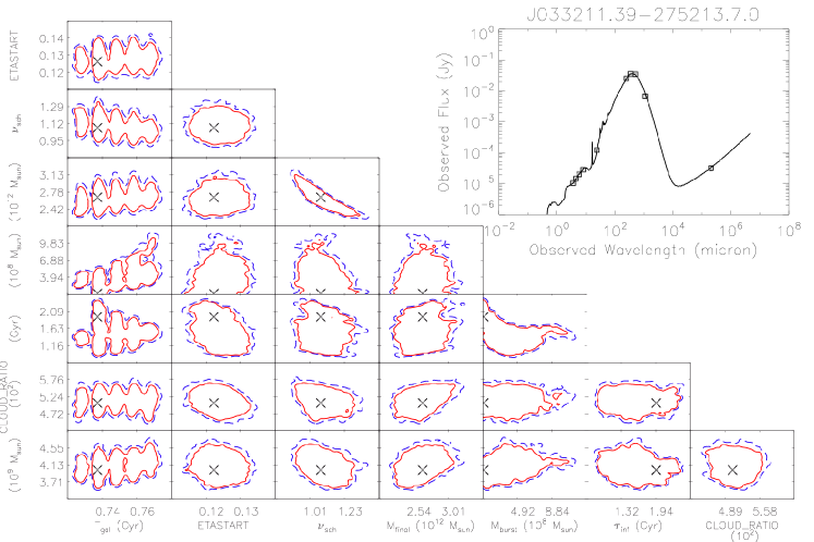
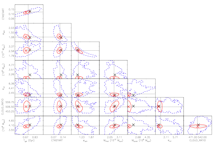
With our GRASIL parameter space as defined above, it is straight-forward to fit our SMGs sample with SATMC. A sample of the final SED produced by SATMC is shown in Figure 5 with a summary of the fitting results in Figure 6 and Tables 5 and 6. An important aspect to note from the parameter-parameter covariances is that many parameters show tight constraints and large degeneracies generally do not exist in our adopted parametrization. The strongest correlations exist between M_final and $\nu_{sch}$ which together set the stellar mass M_∗. In the observed SEDs, the stellar mass is measured through the stellar bump which is most prominent in the IRAC bands. As the IRAC observations have very small flux errors ($\lesssim$1%), this limits parameter space to the narrow range of M_final and $\nu_{sch}$ capable of reproducing the observed fluxes.

Figure 6: Best fit GRASIL models to the SMG sample. Included in each panel are the source ID, redshift used during the fitting (see Table 3), and the ln(L) value of the fit.

Figure 7: Compiled SEDs for the SMG sample. The median SED is given by the solid black line with the grey shaded region indicating the dynamic range between individual SEDs. Left: The composite SEDs overlaid with the average star-formation templates of Kirkpatrick et al. 2012. The photometry used in constructing the $z\sim 2$ SF sample has been included to demonstrate the scatter in the data. Right: The composite SEDs overlaid with median SMG template of Michalowski, Watson & Hjorth 2010 with the dashed lines encompassing the dispersion in the Mickalowski et al. models. Note that these models have not been re-normalized to fit our model set.

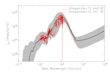
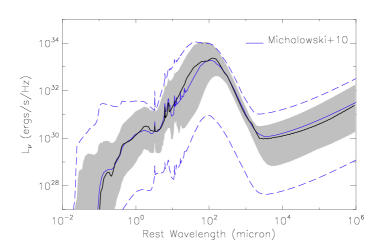
When examining a population of sources, it is often helpful to view the SEDs as a composite and construct an empirical median template. This allows one to easily see trends common in the population including the approximate flux ranges covered by the models and dominate aspects of the SEDs. Figure 7 shows our composite rest-frame GRASIL models along with the median SED of Michalowski, Watson & Hjorth (2010), who fit the SEDs of SMGs using a grid developed from GRASIL, and the composite star-forming SEDs of Kirkpatrick et al. (2012), derived from $z\sim 1$ and $z\sim 2$ sources in GOODS-N and ECDFS with Spitzer IRS spectroscopy. Though Michalowski et al. and Kirkpatrick et al. normalize their fits at specific wavelengths to construct the composite, we have applied no re-normalization to match our SED set. The agreement between our SEDs with those of Mickalowski et al. and Kirkpatrick et al. is immediately apparent. From Kirkpatrick et al., our composite SED best agrees with the $z\sim 2$ star-forming galaxy; not surprising as SMGs peak around $z\sim 2.5$. Our composite also shows excellent agreement with the median Michalowski et al. SED. There are some minor discrepancies between the composites though they are likely attributed to differences in parametrizing the SED. Compared to the Kirkpatrick et al. composites, our SFRs and stellar mass estimates are higher by a factor of $\sim$2 which can readily be explained by the SFH adopted. Regardless, our composite SED is not only able to recover the medians of Kirkpatrick et al. and Michalowski et al. but also encompass the scatter in the observations and dispersion in similar template sets.

Figure 8: Compiled histogram distribution of accepted steps from all fits. Note that the histogram distributions differ slightly from the likelihood distributions but maintain the same general characteristics due to the multi-dimensional nature of the data volume.

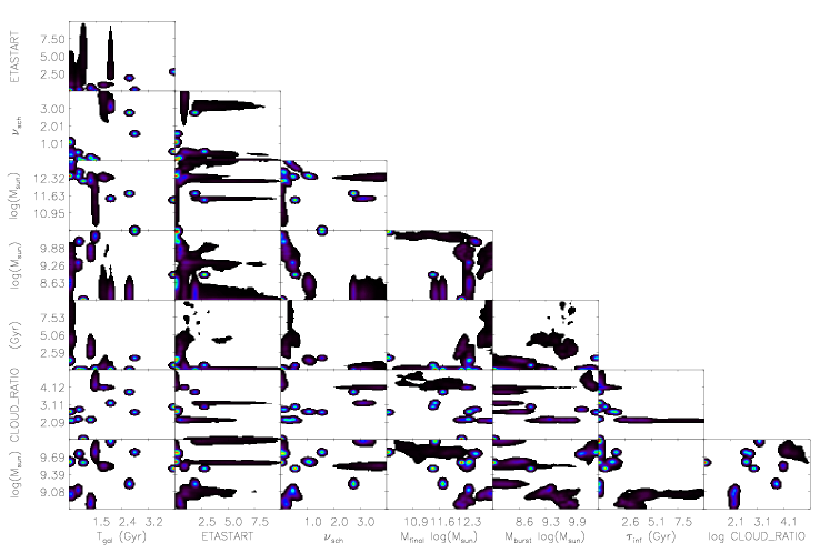
Despite the similar shapes and well defined empirical median of our fitted SEDs, the SMGs in our sample are not heterogeneous in nature and, in fact, occupy large regions of parameter space. Fig. 8 shows that while some areas of parameter space are well constrained (e.g. $\tau_{inf}$ versus T_gal), there is no single set of parameters that may describe our sample as an individual population. Of all our adopted parameters, M_dust shows the tightest constraints (Table 4). This is primarily due to the inclusion of the (sub-)mm observations which are highly sensitive to the total dust mass. Though the parameters $\nu_{sch}$ and M_total had shown tight correlations in individual fits, the composite fits show no signs of the original correlations.

5.4 SMGs and the ’Main-Sequence’ of Galaxy Formation

It is often believed that SMGs must result from powerful starbursts possibility triggered by major mergers. However, these results show a wide range in derived SFRs ($\sim$20-2000 M_⊙ yr^-1) with many below the $\sim$1000 M_⊙ yr^-1 typically assumed for SMGs. Furthermore, the ’merger ratio’ (M_burst/M_final) would also suggest that major mergers are uncommon. This is in agreement with Hayward et al. (2011) who find that starbursts are highly inefficient at boosting the sub-mm flux (e.g. a $\gtrsim$16$\times$ boost in SFR produces $\lesssim$2$\times$ increased sub-mm flux). Indeed, the common trend in our sample is that the bulk of the stellar mass is built from the Schmidt component rather than a ’merger’ triggering a starburst. A more detailed study including a larger sample is needed to further clarify this point. The sources with low SFR could result from source blending giving rise to an enhanced sub-mm flux as also suggested by Hayward et al. Karim et al. (2013) have shown that the brightest LABOCA sources ($S_{850\mu m}\gtrsim 12$ mJy) are composed of multiple, fainter SMGs. For our AzTEC SMG sample, however, the corresponding bright flux limit is $\sim$6.7 mJy (assuming R=$S_{850\mu m}/S_{1.1mm}=1.8$; Chapman et al., 2009) which only applies to the source J033211.39-275213.7, a source with no multiple X-ray detection and derived SFR$\sim$2000 M_⊙ yr^-1. Furthermore, only 2 to 3 out of 12 of our SMGs have multiple potential counterparts (Table 3), none of which correspond to a low SFR source. While source blending is certainly problematic for correctly interpreting multi-wavelength SED fits, it does not have a significant influence in our sample.

Figure 9: SSFR as a function of redshift. The area within the dashed lines represents the main-sequence of galaxies from Elbaz et al. 2011 with galaxies above this limit defined as starbursts. The lower long-dashed line represents the approximate main-sequence relation for our sample accounting for the factor of $\sim$5 difference in stellar masses between the Elbaz et al. sample and those presented here.

Table 7: Comparison of fitted parameters for the source J033213.88-275600.2 using a Salpeter and Chabrier IMF.

IMF	Tgal	etastart	$\nu_{sch}$	Mfinal	Mburst	$\tau_{inf}$	CLOUD_RATIO	Mdust	ln(L)
	Gyr	Gyr		1011 M⊙	109 M⊙	Gyr	M⊙ pc-2	109 M⊙
Salpeter	0.82${}^{+0.01}_{-0.01}$	0.94${}^{+9.03}_{-0.58}$	0.32${}^{+0.43}_{-0.03}$	93.0${}^{+7.0}_{-48.4}$	9.66${}^{+3.36}_{-9.11}$	8.12${}^{+1.87}_{-5.83}$	1.52${}^{+0.20}_{-0.10}$e2	1.11${}^{+0.32}_{-0.27}$	-80.3
Chabrier	0.90${}^{+0.01}_{-0.01}$	0.94${}^{+9.01}_{-0.38}$	0.52${}^{+0.06}_{-0.11}$	88.3${}^{+11.7}_{-7.2}$	1.16${}^{+23.69}_{-1.06}$	0.19${}^{+0.15}_{-0.09}$	1.30${}^{+0.17}_{-0.03}$e2	1.44${}^{+0.20}_{-0.52}$	-102.9

Expanding on this point, we show the specific star formation rate (SSFR=SFR/M_∗) with respect to redshift for our SMG sample in Fig. 9. Elbaz et al. (2011) have suggested an evolution in SSFR for quiescent and starbursting galaxies which follow the general forms SSFR=26$\times t^{-2.2}$ Gyr^-1 and SSFR$>56\times t^{-2.2}$ Gyr^-1, where $t$ is the cosmic time, for quiescent or ’main-sequence’ galaxies and starbursts, respectively. We should point out, however, that the stellar masses used to derive the Elbaz et al. relation are on order $\sim 5\times$ lower than stellar masses in our sample. As a result, only 3 of our SMGs lie above the ’main-sequence’ relation of Elbaz et al. Despite this discrepancy, our SFRs and stellar masses agree with Michalowski, Watson & Hjorth (2010) and the predictions of Hayward et al. (2011); differences in stellar mass derivations can be attributed to differences in the parametrization of the SFRH, IMF (see § 5.4) and stellar evolution tracks (see also Michalowski et al., 2012). Given the uncertainties in determining the stellar mass, we caution against over-interpretation of the SSFRs. However, adjusting for the relative differences in stellar masses, we see that the majority of our sample lie above or near the main-sequence relation while spanning a large range of SSFRs. Overall, these results suggest that there is not a single population that defines our SMG sample; instead, they are homogeneous in origin composed of a mixture of starburst and quiescent galaxies of various ages and SFRHs.

5.5 Comparing Model Parametrizations

Table 8: Comparison of derived parameters for J033213.88-275600.2 using Salpeter and Chabrier IMFs.

IMF	SFR	M∗	SSFR
	M⊙ yr-1	1011 M⊙	Gyr-1
Salpeter	2829.0${}^{+166.7}_{-304.7}$	8.50${}^{+0.97}_{-0.45}$	3.33
Chabrier	3893.4${}^{+192.1}_{-122.5}$	13.47${}^{+1.79}_{-1.94}$	2.89

When developing SED models and deriving the associated parameters, there are certain attributes that must remain fixed in order to keep a consistent parametrization. Examples of these attributes include the IMF, spatial properties like the disk/bulge scale heights and radial distribution, and the form of the SFH. Altering any of these properties changes the very nature of the models and is in no way continuous for MCMC samplers. In Bayesian statistics, it is possible to compare models of different parametrizations through the Bayes factor to determine which model offers the ’best’ fit (e.g. Jefferys, 1961; Weinberg, 2012; Weinberg, Yoon & Katz, 2013). The Bayes factor follows from Bayes’ Theorem and is derived from the ratio of the posteriors for the two models $M_{1}$ and $M_{2}$:

$$\frac{P(M_{1}|{\bf D})}{P(M_{2}|{\bf D})}=\frac{P(M_{1})}{P(M_{2})}\frac{P({\bf D}|M_{1})}{P({\bf D}|M_{2})}.$$ (9)

The Bayes factor is defined as the second term on the right-hand side; the first term is the ratio of the prior probability of each model and is typically set to unity as the models are considered under equal weight. Explicit calculation of the Bayes factor ($B_{12}$) involves integrating the likelihood distributions of each model ($L_{1}({\bf D}|\theta_{1})$ and $L_{2}({\bf D}|\theta_{2})$) with the prior parameter distributions ($\pi_{1}(\theta_{1})$ and $\pi_{2}(\theta_{2})$) according to

$$B_{12}=\frac{P({\bf D}|M_{1})}{P({\bf D}|M_{2})}\frac{\int\pi_{1}(\theta_{1}|M_{1})L_{1}({\bf D}|\theta_{1},M_{1}){\rm d}\theta_{1}}{\int\pi_{2}(\theta_{2}|M_{2})L_{2}({\bf D}|\theta_{2},M_{2}){\rm d}\theta_{2})}.$$ (10)

While there are MCMC and Bayesian based tools available that compute the Bayes factor (e.g. the Bayesian Inference Engine BIE, Weinberg, 2012), such methods are not currently available in SATMC. Instead, we may follow a similar prescription by repeating the SED fits after changing the desired parametrization(s). We provide a brief example of this process by comparing the results obtained with the Salpeter IMF used in our initial fits and those obtained with a Chabrier IMF (Chabrier, 2003). Tables 7 & 8 and show that for the source J033213.88-275600.2 the fitted parameters remain nearly constant except for $\tau_{inf}$ which causes an increase in the derived SFRs and stellar mass while the fitted SEDs are nearly identical (Figure 10). We caution, however, that without results from a full sample and direct computation of the Bayes factor, we can not differentiate between the two IMFs at this time. Without the Bayes factors, one may include secondary observations, i.e. spectroscopy and SED independent estimates of fitted and/or derived parameters, to derive priors and determine which, if any, of the fits best describe all observations.

Figure 10: Best fit GRASIL SEDs for J033213.88-275600.2 using Salpeter (solid) and Chabrier (dashed) IMFs.

5.6 Application of Additional Observations to SED Fits

Figure 11: 68 percent error contours for a simulated GRASIL SED based on the fitted spectrum of J033211.39-275213.7 at z$\sim 4$. The contours are shown for the original AzTEC photometric errors (blue dashed) and improved by a factor of 10 (red solid). The location of the maximum likelihoods for each case are marked by the X’s with values used in construction of the simulated SEDs marked by the dotted lines. For the high-z simulation, improving the AzTEC signal-to-noise provides significantly greater constraints on parameter space.

As mentioned in § 2.2, whenever an SED synthesis routine is used in SATMC, the SEDs for each step are saved along with its location in parameter space and likelihood. Using these ’SED steps’, one can examine the influence of additional or improved photometric data simply by referring back to Eqns. 5 & 8 without having to re-run the entire MCMC fit. This can be exceptionally useful given the long typical run time of a single fit and is best used for examining the influence on parameter space when including low signal-to-noise observations (e.g. LABOCA) or observations one believes will truncate regions of parameter space (e.g. priors on parameters). To examine the full impact of improved or additional observations, it is necessary to repeat the fits as the sampling of likelihood space is wholly dependent on the initial set of observations and relative uncertainties. As an example, we have created simulated GRASIL SEDs based on the best fit parameters of J033211.39-275213.7 ($z\sim 4$). The simulated SED is produced using the same formalism and parametrization described in § 4 & 5.2 and has been sampled at wavelengths corresponding to the actual observations (3.6$\mu$m, 4.5$\mu$m, 5.8$\mu$m, 8.0$\mu$m, 24$\mu$m, 250$\mu$m, 350$\mu$m, 500$\mu$m, 1.1mm). Each band is then assigned the measured flux uncertainties. For one simulation, we have increased the AzTEC signal-to-noise by a factor of 10 ($\sigma_{1.1mm}\sim 0.1$ mJy) – similar to the level of improvement expected with LMT, ALMA and future sub-mm telescopes – whereas the control simulation maintains the original AzTEC signal-to-noise ($\sigma_{1.1mm}\sim$1 mJy). Figure 11 shows the 68 percent contours for the GRASIL fits to the simulated SEDs where we immediately see tighter constraints on fitted parameters for the improved AzTEC photometry. Referring back to Figure 6, we see that the AzTEC photometry is one of the few points beyond the thermal dust peak and along the Rayleigh-Jeans tail of the dust blackbody distribution. At lower redshifts, the Herschel/SPIRE bands become more prominent in the beyond the dusk peak which serves to diminish the impact of improved (sub-)mm photometry. For the most distant galaxies, however, high signal-to-noise (sub-)mm photometry is instrumental for fully constraining the SED shape and its driving parameters, namely its SFRH ($T_{gal}$, $M_{total}$, $M_{burst}$, $\nu_{sch}$, $\tau_{inf}$) and dust content $M_{dust}$. The future observations of SMGs with LMT and ALMA will therefore be paramount to our understanding of high-redshift galaxies.

6 Summary

We have presented the general purpose MCMC-based SED fitting tool SATMC. Utilizing MCMC algorithms, the code is able to take any set of SED templates or models of the user’s choice and return the requested best fit parameter estimates in addition to the posterior parameter distribution which can be used to construct confidence levels and unveil parameter correlations. In testament to SATMC’s flexibility, we have provide a series of test cases comparing SATMC with traditional least-squares methods where SATMC recovers best fit values similar to those from traditional methods. Furthermore, we show that SATMC is capable of reproducing the set of input parameters from a simulated SED which serves to prove SATMC’s adaptability and reliability.

Highlighting SATMC’s scientific value, we also provide the best-fit GRASIL models to a sample of AzTEC submillimetre galaxies in the GOODS-S field. These fits indicate that while some parameters exhibit obvious and strong correlations in individual SED fits, such correlations are absent when constructing the population. Furthermore, these sources appear to span a wide dynamic range of fitted and derived parameters, specifically when considering their derived SFRs ($\sim$30-3000 M_⊙ yr^-1) and stellar masses ($\sim 10^{10}-10^{12}$ M_⊙); these results agree both with the previous GRASIL-based SEDs of Michalowski, Watson & Hjorth (2010) and simulations of SMGs (Hayward et al., 2011). We also provide a brief demonstration of the impact of improved photometric data on the best fit results. Increasing the signal-to-noise of the AzTEC photometry provides significantly greater constraints on fitted parameters and highlights the need to obtain deeper (sub)-mm data. As observations, the complexity of models and the desire to obtain more detailed information from model fits increase, the approach of tools like SATMC will be required in both observational and theoretical astronomy in order to refine our understanding of the Universe and its constituents.

References

- Acquaviva, Gawiser & Guaita (2011) Acquaviva V., Gawiser E., Guaita L. 2011, ApJ, 737, 47
- Acquaviva, Gawiser & Guaita (2012) Acquaviva V., Gawiser E., Guaita L. 2012, IAUS, 284, 42
- Atchade & Rosenthal (2005) Atchade Y.F., Rosenthal J.S. 2005, Bernoulli, 11, 815
- Benitez (2000) Benitez N. 2000, ApJ, 536, 571
- Blain et al. (2002) Blain A.W., Smail I., Ivison R.J., Kneib J.-P., Frayer D.T. 2002, Physics Reports, 369, 111
- Blain et al. (2004) Blain A.W., Chapman S.C., Smail I., Ivison R. 2004, ApJ, 611, 52
- Bolzonella, Miralles & Pelló (2000) Bolzonella M., Miralles J.-M., Pelló R. 2000, A&A, 363, 476
- Brammer, van Dokkum & Coppi (2008) Brammer G.B., van Dokkum P.G., Coppi P. 2008, ApJ, 686, 1503
- Bruzual & Charlot (1993) Bruzual A., Charlot S. 1993, ApJ, 405, 538
- Bruzual & Charlot (2003) Bruzual A., Charlot S. 2003, MNRAS, 344, 1000
- Calzetti et al. (2000) Calzetti D., Armus L., Bohlin R.C., Kinney A.L., Koornneef J., Storchi-Bergmann T. ApJ, 533, 682
- Cardamone et al. (2010) Cardamone C.N. et al. 2010, ApJS, 189, 270
- Chabrier (2003) Chabrier G. 2003, PASP, 115, 763
- Chapman et al. (2005) Chapman S.C., Blain A.W., Smail I., Ivison R.J. 2005, ApJ, 622, 772
- Chapman et al. (2009) Chapman S.C., Blain A.W., Ibata R., Ivison R.J., Smail I., Morrison G. 2009, ApJ, 691, 560
- Chib & Jeliazkov (2001) Chib O., Jeliazkov I. 2001, J. Am. Stat. Assoc.
- Coppin et al. (2006) Coppin K.E. et al. 2006, MNRAS, 372, 1621
- Dahlen et al. (2010) Dahlen T. et al. 2010, ApJ, 724, 425
- Dahlen et al. (2013) Dahlen T. et al. 2013, ApJ accepted, arXiv:1308.5353
- Damen et al. (2011) Damen M. et al. 2011, ApJ, 727, 1
- Draine & Lee (1984) Draine B.T., Lee H.M. 1984, ApJ, 258, 89
- Earl & Deem (2005) Earl D.J., Deem M.W. 2005, Physical Chemistry Chemical Physics, 7, 3910
- Efstatiou, Rowan-Robinson & Siebenmorgen (2000) Efstathiou A., Rowan-Robinson M., Siebenmorgen R. 2000, MNRAS, 313, 734
- Elbaz et al. (2011) Elbaz D. et al. 2011, A&A, 533, 119
- Feigelson & Nelson (1985) Feigelson E.D., Nelson P.I. 1985, ApJ, 293, 192
- Gawiser (2009) Gawiser E. 2000, Nes Astronomy Review, 53, 50
- Geman & Geman (1984) Geman S., Geman D. 1984, IEE Transactions on Pattern Analysis and Machine Intelligence, 6, 721
- Gelman & Rubin (1992) Gelman A., Rubin D. 1992, Statistical Science, 7, 457
- Gelman, Roberts & Gilks (1995) Gelman A., Roberts G.O., Gilks W.R. 1996, Bayesian Statistics 5, eds. Bernado J.M, Berger J., Dawid A.P., Smith A.F.M, Oxford: Oxford University Press
- Geweke (1992) Geweke J. 1992, Bayesian Statistics 4, eds. Bernardo J.M., Berger J., Dawid A.P., Smith A.F.M., Oxford: Oxford University Press
- Geyer (1991) Geyer C.J. 1991, Computing Science and Statistics: Proc. 23rd Symp. Interface, 156
- Geyer (1992) Geyer C.J. 1992, Statistical Science, 7, 4, 473
- Giavalisco et al. (2004) Giavalisco M. et al. 2004, ApJ, 600, 93
- Gilks, Richardson & Spiegelhalter (1996) Gilks W.R., Richardson S., Spiegelhalter D. 1996, Markov Chain Monte Carlo in Practice, eds. Gilks W.R., Richardson S., Spiegelhalter D., London: Chapman and Hall.
- Hastings (1970) Hastings W.K. 1970, Biometrika, 57, 97
- Hayward et al. (2011) Hayward C.C., Keres D., Jonsson P., Narayanan D., Cox T.J., Hernquist L. 2011, ApJ, 743, 159
- Hodge et al. (2013) Hodge J.A. et al. 2013, ApJ, 768, 91
- Hughes et al. (1998) Hughes D.H. et al. 1998, Nature, 394, 241
- Iglesias-Páramo et al. (2007) Iglesias-Páramo J. et al. 2007, ApJ, 670, 279
- Ilbert et al. (2006) Ilbert O. et al. 2006, A&A, 457, 841
- Isobe, Feigelson & Nelson (1986) Isobe T., Feigelson E.D, Nelson P.I. 1986, ApJ, 306, 490
- Jefferys (1961) Jefferys H. 1961, Theory of Probability, 3rd edition, Oxford, University Press
- Johnson et al. (2013) S.P. Johnson et al. 2013, MNRAS, arXiv:1302.0842431, 662
- Karim et al. (2013) Karim A. et al. 2013, MNRAS, 432, 2
- Kellermann et al. (2008) Kellermann K. I., Fomalont E. B., Mainieri V., Padovani P., Rosati P., Shaver P., Tozzi P., Miller N., 2008, ApJS, 179, 71
- Kennicutt (1998) Kennicutt R.C. 1998, ARAA, 36, 189
- Kirkpatrick et al. (2012) Kirkpatrick A. et al. 2012, ApJ, 759, 139
- Kodama, Bell & Bower (1999) Kodama T., Bell E.F., Bower R.G 1999, MNRAS, 302, 152
- Kroupa (2001) Kroupa P. 2001, MNRAS, 322,231
- Lewis & Bridle (2002) Lewis A., Bridle S. 2002, PRD, 66, 103511
- Mackay (2003) Mackay D. 2003, Information Theory, Inference, and Learning Algorithms, Cambridge Univ., Cambridge
- Marconi et al. (2004) Marconi A., Risaliti G., Gilli R., Hunt L.K., Maiolino R., Salvati M. 2004, MNRAS, 351, 169
- Metroplois et al. (1953) Metropolis N., Rosenbluth A.W., Rosenbluth M.N., Teller A.H., Teller E. 1953, J. Chemical. Phys., 21, 1087
- Michalowski, Watson & Hjorth (2010) Michaloski M.J., Watson D., Hjorth J. 2010, ApJ, 712, 942
- Michalowski et al. (2012) Michalowski M.J., Dunlop J.S., Cirasuolo M., Hjorth J., Hayward C.C., Watson D. 2012, A&A, 541, 85
- Nenkova et al. (2008) Nenkova M., Sirocky M.M., Nikutta R., Ivezic Z., Elitzur M. 2008, ApJ, 685, 160
- Noll et al. (2009) Noll S., Burgarella D., Giovannoli E., Buat V., Marcillac D., Muñoz-Mateos J.C. 2009, A&A, 507, 1793
- Oliver et al. (2012) Oliver S.J. et al. 2012, MNRAS, 424, 1614
- Persic et al. (2004) Persic M., Rephaeli Y., Braito V., Cappi M., Della Ceca R., Franceschini A., Gruber D.E. 2004, A&A, 419, 849
- Pirzkal et al. (2012) Pirzkal N., Rothberg B., Nilsson K.K., Finkelstein S., Koekemoer A., Malhotra S., Rhoads J. 2012, ApJ, 748, 122
- Press et al. (1992) Press W.H., Teukolsky S.A., Vetterling W.T., Flannery B.P. 1992, Numerical Recipes in C: The Art of Scientific Computing, 2nd edn. Cambridge Univ., Cambridge
- Raftery & Lewis (1992) Raftery A.E., Lewis, S. 1992, Bayesian Statistics 4, eds. Bernardo J.M., Berger J., Dawid A.P., Smith A.F.M., Oxford: Oxford University Press
- Rafferty et al. (2011) Rafferty D.A., Brandt W.N., Alexander D.M., Xue Y.Q., Bauer F.E., Lehmer B.D., Luo B., Papovich, C. 2011, ApJ, 742, 3
- Roberts, Gelman, & Gilks (1997) Roberts G.O., Gelman A., Gilks W. 1997, Ann. Applied Prob., 7, 110
- Roberts & Rosenthal (2001) Roberts G.O., Rosenthal J.S. 2001, Statistical Science, 16, 351
- Sajina et al. (2006) Sajina A., Scott D., Dennefeld M., Dole H., Lacy M., Lagache G. 2006, MNRAS, 369, 939
- Salpeter (1955) Salpeter E.E. 1955, ApJ, 121, 161
- Sawicki (2012) Sawicki M. 2012, PASP, 124, 1208
- Scott et al. (2010) Scott K.S. et al. 2010, MNRAS, 405, 2260
- Serra et al. (2011) Serra P., Amblard A., Temi P., Nurgarella D., Giovannoli E., Buat V., Noll S., Im S. 2011, ApJ, 740, 22
- Siebenmorgen et al. (2004) Siebenmorgen R., Freudling W., Krügel E., Haas M. 2004, A&A, 421, 129
- Siebenmorgen & Krügel (2007) Siebenmorgen R., Krügel E. 2007, A&A, 461, 445
- Silva et al. (1998) Silva L., Granato G.L., Bressan A., Danese L. 1998, ApJ, 509, 103
- Swinbank et al. (2010) Swinbank A.M. et al. 2010, Nature, 464, 733
- Verde et al. (2003) Verde L. et al. 2003, ApJS, 148, 195
- Weinberg (2012) Weinberg M.D. 2012, arXiv:1203.3816
- Weinberg, Yoon & Katz (2013) Weinberg M.D., Yoon I., Katz N. 2013, arXiv:1301.3156
- Wei et al. (2009) Wei A. et al. 2009, ApJ, 707, 1201
- Xue et al. (2011) Xue Y.Q. et al. 2011, ApJS, 195, 10
- Yun et al. (2012) Yun M.S. et al. 2012, MNRAS, 420, 957