Noiseless amplification of weak coherent fields without external energy

Abstract

According to the fundamental laws of quantum optics, noise is necessarily added to the system when one tries to clone or amplify a quantum state. However, it has recently been shown that the quantum noise related to the operation of a linear phase-insensitive amplifier can be avoided when the requirement of a deterministic operation is relaxed. Nondeterministic noiseless linear amplifiers are therefore realizable. Usually nondeterministic amplifiers rely on using single photon sources. We have, in contrast, recently proposed an amplification scheme in which no external energy is added to the signal, but the energy required to amplify the signal originates from the stochastic fluctuations in the field itself. Applying our amplification scheme, we examine the amplifier gain and the success rate as well as the properties of the output states after successful and failed amplification processes. We also optimize the setup to find the maximum success rates in terms of the reflectivities of the beam splitters used in the setup. In addition, we discuss the nonidealities related to the operation of our setup and the relation of our setup with the previous setups.

1 Introduction

Quantum noise is unavoidably added into the signal in any conventional amplification process [1]. This follows from the linearity and unitary evolution of quantum mechanics and guarantees against unphysical situations violating the Heisenberg uncertainty principle. However, it has been shown that the addition of quantum noise can be circumvented by implementing the amplification process nondeterministically [2, 3, 4, 5]. This results in a process in which conditional quantum operations, such as a sequence of single-photon addition and subtraction, are applied to the optical field [6, 7, 8]. Typically, the addition and subtraction of photons are experimentally implemented by using single-photon light sources, beam splitters, and photodetectors [2, 3, 4, 5]. We have, in contrast, recently proposed an amplification setup in which, the energy required to amplify the signal does not originate from external energy sources, such as single-photon sources, but the required energy comes from the stochastic fluctuations in the field itself [9]. In quantum communications and metrology, the noiseless amplification schemes could become an essential tool to recover information transmitted over lossy channels or to enhance the discrimination between partially overlapping quantum states [2, 10].

In this paper, we analyze our recently proposed amplification scheme, which adds no external energy to the optical signal. The scheme consists of beam splitters and photodetectors that are routinely used in experiments and a quantum nondemolition (QND) measurement [11, 12, 13] that is not as common but nevertheless has several experimental implementations [14, 15, 16]. We start by a short summary of the basic principles of noiseless amplification and by a description of our amplification setup. By optimizing the setup, we find the maximum success rates in terms of the reflectivities of the beam splitters used in the setup. This is followed by a discussion of the nonidealities and the realizatization of the QND measurement related to the operation of our setup. We also investigate the statistics of the output states after successful and failed amplification processes. Furthermore, we discuss the relation of our setup with the previous setups.

2 Amplification scheme

The proposed amplification scheme, illustrated in Fig. 1, utilizes the energy fluctuations of the initial field to replace the single-photon source that would otherwise be needed as in the scheme suggested by Zavatta et al. [2]. In our scheme, a similar action is obtained by a configuration where the successful subtraction of a single photon from the initial field by a beam splitter is verified by a QND measurement, which is followed by adding the photon back to the field by the second beam splitter if no photons are detected at photodetector PD1. Finally, another photon is subtracted from the field at the third beam splitter, if photodetector PD2 detects a photon. The final output state resulting from these events is an amplified coherent state with high fidelity, but this output state only occurs when the QND, PD1, and PD2 detectors detect 1, 0, and 1 photons, respectively.

The action of an ideal noiseless amplifier for coherent states can be described as $|\alpha\rangle\rightarrow|g\alpha\rangle$, where $|\alpha\rangle$ is the initial coherent field, $|g\alpha\rangle$ is the amplified field, and $g$ is the gain of amplification. This operation cannot be implemented by conventional amplifiers, but it can be approximated nondeterministically. It has been shown that the operator $\hat{G}=\hat{a}\hat{a}^{\dagger}$, where $\hat{a}$ and $\hat{a}^{\dagger}$ are the annihilation and creation operators of the field, approximates the action of amplification for weak coherent fields with nominal gain $g=2$ [17]. The scheme suggested by Zavatta et al. [2] is based on this. The same outcome is also obtained by an operator $\hat{G}^{\,\prime}=\hat{a}\hat{a}^{\dagger}\hat{a}$ implemented by the setup used in this paper because the coherent input field $|\alpha\rangle$ is an eigenstate of $\hat{a}$.

The main difference between the presented scheme and the scheme succested by Zavatta et al. [2] is the QND measurement. In general, a QND measurement is a detection process, in which the detected photon is not destructed as in the case of conventional photodetectors. Thus, the process should be repeatable. As stated by the laws of quantum mechanics, the measured state is projected into an eigenstate corresponding to the measurement result. QND measurements can be used as very sensitive probes of small perturbations acting on a system. In addition, QND measurements are also used for unlimited distribution of optical signals [18]. Various schemes for QND measurements with different physical systems have been experimentally realized [14, 15, 16, 11, 12, 13]. For example, Guerlin et al. have observed a step-by-step decay of a cavity field by non-destructively measuring the photon number of a field stored in a cavity [16]. More recently, the same group completed another experiment of field damping and measurement of Fock state lifetimes by QND photon counting in a cavity [19]. A closely related work has also been performed on a superconducting quantum circuit [20].

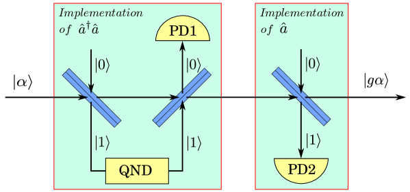
Figure 1: (Color online) A schematic illustration of the noiseless amplification of a weak coherent field. First, a single photon is subtracted from the field, then added back to the field, and finally again subtracted from the field. This sequence is also described by the operator $\hat{a}\hat{a}^{\dagger}\hat{a}$.

2.1 Output field of the amplifier

The output fields of our setup have been calculated using the standard Wigner function formalism. The Wigner function of the initial coherent field $|\alpha\rangle$ is [21]

$$W_{\mathrm{coh}}(x,p)=\frac{1}{\pi\hbar}\exp\!\Big{[}-(\kappa x-\sqrt{2}\mathrm{Re}\alpha)^{2}-\left(\frac{p}{\hbar\kappa}-\sqrt{2}\mathrm{Im}\alpha\right)^{2}\Big{]},$$ (1)

where $x$ and $p$ are position and momentum quadratures of the field, $\alpha$ is a complex variable defining the coherent field amplitude, $\kappa$ is the spring constant of the field oscillator, and $\hbar$ is the reduced Planck constant. When plotting the Wigner functions, it is conventional to set $\hbar=\kappa=1$ [21].

The entangled Wigner function $W_{\mathrm{BS}}$ emerging as a result from fields $W_{\mathrm{field1}}$ and $W_{\mathrm{field2}}$ interfering on a beam splitter is given by [22, 23]

$$W_{\mathrm{BS}}(x_{1},p_{1},x_{2},p_{2})=W_{\mathrm{field1}}(tx_{1}+rx_{2},tp_{1}+rp_{2})W_{\mathrm{field2}}(tx_{2}-rx_{1},tp_{2}-rp_{1}),$$ (2)

where $x_{1}$, $p_{1}$, $x_{2}$, and $p_{2}$ are the position and momentum quadratures of the transmitted and reflected fields and the beam splitter reflection and transmission coefficients $r$ and $t$ obey the relation $r^{2}+t^{2}=1$. In our notation $W_{\mathrm{field1}}$ is the field incident to the beam splitter from the left and transmitted field quadratures refer to the field emerging from the beam splitter to the right in Fig. 1.

The probability of detecting $n$ photons on the reflected field (the field that emerges from the beam splitter and travels vertically in Fig. 1) can be expressed as

$$P(n)=2\pi\hbar\int W_{\mathrm{BS}}(x_{1},p_{1},x_{2},p_{2})W_{n}(x_{2},p_{2})\,dx_{1}\,dp_{1}\,dx_{2}\,dp_{2},$$ (3)

where $W_{n}$ is the Wigner function of the $n$-photon Fock state $|n\rangle$, to which the reflected field collapses after the detection, and is expressed as [21]

$$W_{n}(x,p)=\frac{(-1)^{n}}{\pi\hbar}\exp\!\Big{[}-(\kappa x)^{2}-\left(\frac{p}{\hbar\kappa}\right)^{2}\Big{]}L_{n}\Big{[}2(\kappa x)^{2}+2\left(\frac{p}{\hbar\kappa}\right)^{2}\Big{]},$$ (4)

where $L_{n}(x)$ denotes a Laguerre polynomial of degree $n$. After detecting $n$ photons on the reflected field, the transmitted field collapses to

$$W_{\mathrm{T}}(x_{1},p_{1})=\frac{2\pi\hbar}{P(n)}\int W_{\mathrm{BS}}(x_{1},p_{1},x_{2},p_{2})W_{n}(x_{2},p_{2})\,dx_{2}\,dp_{2}.$$ (5)

The collapsed transmitted field is then used as the input for the second beam splitter. Despite the physical difference between the QND and PD, their effect on the transmitted field is exactly the same, and to calculate the final output of the setup Eqs. (2)–(5) are applied for the remaining two beam splitters as described in more detail below. For simplicity, we have made the usual assumption that the photodetectors PD1 and PD2 are ideal. The same assumption is also made for the QND since measurements made with QND detectors have been reported to yield single-photon Fock states with good accuracy [14, 15, 16, 11, 12, 13]. We will discuss the nonidealities more thoroughly in section 2.4.

The details of the analysis of how the state is propagated through the setup resulting in the conditional state of interest are as follows. In the first beam splitter, the initial coherent field $|\alpha\rangle$ in Eq. (1) is mixed with a vacuum state $|0\rangle$ [a zero-photon Fock state $n=0$ in Eq. (4)] using Eq. (2). Then, one photon is measured by the QND detector. The probability for this and the transmitted field are given by Eqs. (3) and (5) with $n=1$. In the second beam splitter, the transmitted field is mixed with a single-photon Fock state using Eq. (2) since a photon coming from the QND detector is added to the field. No photons are measured by photodetector PD1. The probability for this and the transmitted field are given by Eqs. (3) and (5) with $n=0$. In the third beam splitter, a photon is subtracted from the field. This is performed by mixing the field with a vacuum state using Eq. (2) and using Eqs. (3) and (5) with $n=1$ for calculating the probability and the transmitted field that is the final output state of the setup. The total probability for this successfully amplified output state $P_{\mathrm{succ}}$ is the product of the mentioned three photon detection probabilities given by

$$P_{\mathrm{succ}}=(1+|t_{1}t_{2}t_{3}\alpha|^{2}(3+|t_{1}t_{2}t_{3}\alpha|^{2}))|r_{1}r_{2}r_{3}\alpha|^{2}e^{|t_{1}t_{2}t_{3}\alpha|^{2}-|\alpha|^{2}},$$ (6)

where $r_{i}$ and $t_{i}$, $i=1,2,3$, are reflectivities and transmittivities of the beam splitters in the setup obeying $r_{i}^{2}+t_{i}^{2}=1$.

2.2 Effective gain and fidelity of the amplified state

In the calculations depending on the parameters of the setup, effective gain values different from the nominal gain of 2 can be found. The effective gain can be defined as the ratio of the expectation values of the annihilation operator $\hat{a}$ for the output and input fields [2]

$$g_{\mathrm{eff}}=\frac{|\langle\hat{a}_{\mathrm{out}}\rangle|}{|\langle\hat{a}_{\mathrm{in}}\rangle|},$$ (7)

which corresponds to the effective amplification of the electric-field amplitude. In the Wigner function formalism, the expectation value of the annihilation operator can be calculated using the operator correspondence relation as [24]

$$\langle\hat{a}\rangle=\int\left[\frac{\kappa}{\sqrt{2}}\left(x+\frac{i\hbar}{2}\frac{\partial}{\partial p}\right)+\frac{i}{\sqrt{2}\hbar\kappa}\left(p-\frac{i\hbar}{2}\frac{\partial}{\partial x}\right)\right]W(x,p)\,dx\,dp.$$ (8)

The calculations produce the following expression for the effective gain:

$$g_{\mathrm{eff}}=\frac{t_{1}t_{2}t_{3}(2+4|t_{1}t_{2}t_{3}\alpha|^{2}+|t_{1}t_{2}t_{3}\alpha|^{4})}{1+3|t_{1}t_{2}t_{3}\alpha|^{2}+|t_{1}t_{2}t_{3}\alpha|^{4}}.$$ (9)

It is also useful to quantify how much the output state differs from an ideally amplified coherent state. A practical measure for this purpose is the fidelity $F$, which is the overlap between the states calculated using Wigner functions $W_{1}$ and $W_{2}$ of the compared fields [25]

$$F(W_{1},W_{2})=2\pi\hbar\int W_{1}(x,p)W_{2}(x,p)\,dx\,dp.$$ (10)

The fidelity obtained for the successfully amplified field with respect to a coherent field $|g_{\mathrm{eff}}\alpha\rangle$ is

$$F_{\mathrm{eff}}=\frac{(1+2g_{\mathrm{eff}}t_{1}t_{2}t_{3}|\alpha|^{2}+g_{\mathrm{eff}}^{2}t_{1}^{2}t_{2}^{2}t_{3}^{2}|\alpha|^{4})e^{-(g_{\mathrm{eff}}^{2}-t_{1}t_{2}t_{3})^{2}|\alpha|^{2}}}{1+3|t_{1}t_{2}t_{3}\alpha|^{2}+|t_{1}t_{2}t_{3}\alpha|^{4}}.$$ (11)

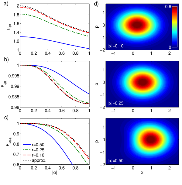
Figure 2: (Color online) (a) Effective gain as a function of the input field amplitude for three different beam splitter reflectivities and for the analytic low reflectivity approximation used by Zavatta et al. [2]. (b) The effective fidelity calculated with respect to a coherent field $|g_{\mathrm{eff}}\alpha\rangle$. (c) The fidelity calculated with respect to an ideally amplified field $|2\alpha\rangle$ for comparison with the results obtained by Zavatta et al. [2]. (d) The contour plots of the Wigner functions for three amplified coherent fields with different input amplitudes when the beam splitter reflectivity is $r=0.4$.

The effective gain, fidelity, and Wigner functions of successfully amplified fields are presented in Fig. 2 as a function of the input field amplitude. In Fig. 2(a) the effective gain is very close to the nominal gain value $g=2$ for small values of $|\alpha|$ and $r$. As the input field amplitude or the beam splitter reflectivity increases, the gain decreases. Increasing the input field amplitude results in the reduction of the effective fidelity $F_{\mathrm{eff}}$ as shown in Fig. 2(b), where the fidelity is calculated with respect to a coherent field $|g_{\mathrm{eff}}\alpha\rangle$. However, the reduction of fidelity can be partly compensated by increasing the beam splitter reflectivity. Figure 2(c) shows the fidelity calculated with respect to an ideal maximally amplified coherent field $|2\alpha\rangle$ for comparison with the results obtained by Zavatta et al. [2] for the setup, including a specific single-photon source. The values for this ideal fidelity $F_{\mathrm{ideal}}$ decrease faster than the effective fidelities $F_{\mathrm{eff}}$ in Fig. 2(b) due to the reduction in $g_{\mathrm{eff}}$ for stronger input fields. Thus $F_{\mathrm{eff}}$ is a better measure for the quality of the resulting output field. One can also see that $F_{\mathrm{ideal}}$ decreases when the beam splitter reflectivity increases while the opposite is true for $F_{\mathrm{eff}}$. This is also due to the reduction in the effective gain. The contour plots in Fig. 2(d) demonstrate how the Wigner function deforms in the amplification. For small initial field amplitudes, the output field is very close to a pure coherent field, but it increasingly deviates from a coherent state when the initial field amplitude increases.

2.3 Optimizing the scheme

Next we investigate how to optimize the probability of successful amplification while maintaining a given effective gain. The optimization problem for maximizing the probability of successful amplification [Eq. (6)] with a constraint requiring the effective gain [Eq. (9)] exceeding a threshold value $g_{\mathrm{eff,0}}$ can be presented as

$$\max_{g_{\mathrm{eff}}\geq g_{\mathrm{eff,0}}}P_{\mathrm{succ}}(|\alpha|,r_{1},r_{2},r_{3}).$$ (12)

Here, $|\alpha|$ is the input field amplitude and the beam splitter reflectivities are $r_{1}$, $r_{2}$, and $r_{3}$. The four-dimensional nonlinear optimization problem in Eq. (12) was solved using a barrier function method [26]. For a certain $g_{\mathrm{eff,0}}$, one finds a single maximum $P_{\mathrm{opt}}$ with an optimal input field amplitude $|\alpha|_{\mathrm{opt}}$ and beam splitter reflectivities $r_{\mathrm{1,opt}}$, $r_{\mathrm{2,opt}}$, and $r_{\mathrm{3,opt}}$. The optimization problem was solved multiple times changing the minimum effective gain parameter $g_{\mathrm{eff,0}}$. It was found that at the optimum all the beam splitter reflectivities have the same value $r_{\mathrm{i,opt}}=r_{\mathrm{opt}}$, $i=1,2,3$.

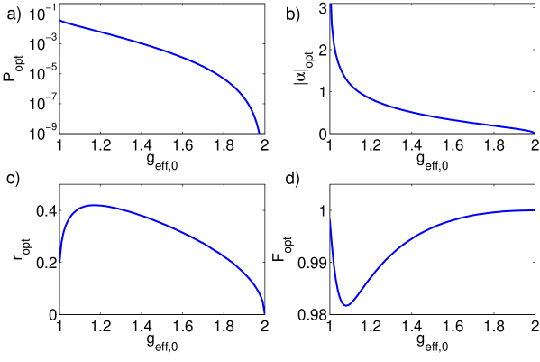
Figure 3: (Color online) Probability of successful amplification was maximized in an effective gain constrained optimization problem. The optimal (a) probability of successful amplification $P_{\mathrm{opt}}$, (b) the input field amplitude $|\alpha|_{\mathrm{opt}}$, (c) the beam splitter reflectivity $r_{\mathrm{opt}}$, and (d) the output field fidelity $F_{\mathrm{opt}}$ are plotted as a function of the required minimum effective gain parameter $g_{\mathrm{eff,0}}$.

Figure 3 shows how the optimized probability of successful amplification $P_{\mathrm{opt}}$, the input field amplitude $|\alpha|_{\mathrm{opt}}$, the beam splitter reflectivity $r_{\mathrm{opt}}$, and the fidelity of the successfully amplified state $F_{\mathrm{opt}}$ evolve as a function of the minimum effective gain parameter $g_{\mathrm{eff,0}}$. The probability of successful amplification in Fig. 3(a) decreases exponentially when the effective gain increases. For instance, if one wants to have an effective gain of 1.4, the maximum success probability of $10^{-3}$ is achievable with $|\alpha|_{\mathrm{opt}}=0.51$ and $r_{\mathrm{opt}}=0.38$. For comparison, Ferreyrol et al. [3, 4] reported success rates of order $10^{-2}$ for a conventional scheme based on quantum scissors [27]. However, their scheme required a single photon source whose effect is not included in the reported success rates. Thus the obtained values can not be directly compared. In Fig. 3(b) one sees that for useful values of $g_{\mathrm{eff,0}}$ the optimal input field amplitude is limited to $|\alpha|_{\mathrm{opt}}<1$. The optimal beam splitter reflectivity in Fig. 3(c) has a maximum $r_{\mathrm{opt}}=0.42$ at the effective gain $g_{\mathrm{eff,0}}=1.18$ and it approaches zero when the required effective gain approaches 2. The fidelity curve in Fig. 3(d) has a minimum $F_{\mathrm{opt}}=0.982$ at $g_{\mathrm{eff,0}}=1.08$. In the nominal gain limit, the fidelity approaches unity.

2.4 QND measurement and other nonidealities

In the calculations of the probability of successful amplification in equation (6), the photodetectors and the QND measurement were assumed to be perfect. In real measurements, this is not the case, but the obtained success probability must be multiplied with the success probabilities of individual photodetectors and the QND measurement. Absorptive single photon detection is possible with efficiencies up to $\sim$90% for visible spectrum and $\sim$95% for near-infrared waves [28, 29, 30]. In addition, Munro et al. reported efficiency of $\sim$99% for the quantum nondemolition measurement [14]. Thus, the magnitude of the real success probabilities is somewhat smaller but still of the same order as the ideal probabilities calculated in this work.

In addition to the success probabilities, one can consider the fidelity of the output states produced by the setup. In the calculations, it was assumed that the initial state is a perfect coherent state and in photon addition and subtraction, the detected beam is projected into a perfect Fock state. In addition, the beam splitters are assumed to be perfect. However, certainly there are experimental inefficiencies that should be taken into account when calculating the fidelities of the output states. Conventional photodetectors do not have any effect on the output state fidelities, but their efficiencies only affect the probabilities of detecting the output states correctly. In contrast, the QND detector can also affect the output states since the measured photon is later added back to the field. QND measurements have been reported to project the field onto Fock states with high fidelity [19], but to the authors’ knowledge, no exact values for the fidelities of the produced Fock states have been reported.

There are at least two suitable implementations for the QND measurement in our amplification scheme: the scheme based on cross-Kerr effect [14] and the scheme based on using atoms in an optical cavity [15]. These schemes are presented in Fig. 4. In the cross-Kerr nonlinearity based scheme in Fig. 4(a), the refractive index of the cross-Kerr medium is altered by the intensity of the signal beam. The probe beam experiences a phase shift that can be detected. The phase shift is proportional to the photon number of the signal beam, and thus the photon number of the signal beam can be determined. Also, in the atom and cavity based scheme in Fig. 4(b), the phase shift experienced by the probe beam depends on the photon number of the signal beam, based on which the photon number of the signal beam can be determined.

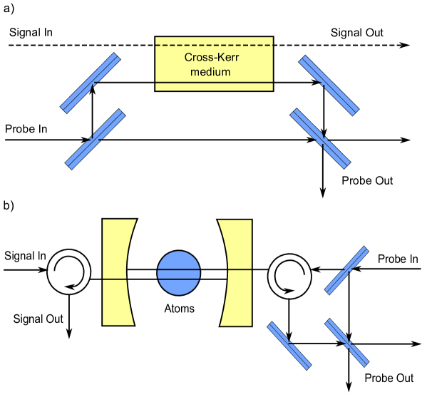
Figure 4: (Color online) Schemes for the implementation of the QND measurement. (a) Measurement scheme based on cross-Kerr effect [14]. The intensity of the signal beam alters the refractive index experienced by the probe beam. This results in a phase shift on the probe beam, based on which the photon number of the signal beam can be determined. (b) Measurement scheme based on using atoms in an optical cavity [15]. The probe beam experiences a phase shift depending on the photon number of the signal beam on the cavity. Rotating arrows indicate optical circulators [11].

2.5 Failed amplification

So far, we have only discussed the case of successful amplification. For completeness, we next analyze the other possible output states. If the initial field is weak and the beam splitter reflectivities are $<0.5$, the probability that any of the photodetectors detects more than one photon is typically $<10^{-2}$. This probability is not completely negligible but since it is still small and the occurrence of these processes can be detected, we can focus on the processes where only at most one photon is detected at a time. These single photon processes and the corresponding eight possible output states are described in Table 1. The output states can be experimentally identified by photon detection measurement outcomes. The first state is the successfully amplified field and the last row shows the probability that more than one photon is detected by some of the photodetectors.

The fidelities in Table 1 clearly show that states from 5 to 8 are exactly coherent. This can be understood by considering what happens if the first photon subtraction fails. In this case, the output from the first beam splitter can be shown to be $|t\alpha\rangle$, which is a perfectly coherent field. This further means that at beam splitters 2 and 3, only single-photon subtraction or no photon subtraction can take place. Both operations result in coherent fields, albeit with reduced amplitude. This is because the photon subtractions only decrease the amplitude and keep the state coherent since coherent states are eigenstates of the annihilation operator [7, 31]. The states 3 and 4 are not exactly coherent since, in these cases, the input field arriving to the second beam splitter from the QND device is a single-photon Fock state producing superposition states at the output.

Table 1: Photon detection measurement outcomes, amplitude expectation values $|\langle\hat{a}\rangle|$, degradations of fidelities $1-F_{\mathrm{eff}}$, and probabilities $P$ for possible single-photon process output states of the amplification setup with $g_{\mathrm{eff}}=1.4$. The initial field is a coherent field with $|\alpha|=0.5$ and the reflectivity of the beam splitters is $r=0.4$. Successful amplification corresponds to the first state.

	Measurements
State	QND	PD1	PD2	$|\langle\hat{a}\rangle|$	$1-F_{\mathrm{eff}}$	$P$
1	1	0	1	0.686	$4.84\times 10^{-3}$	$1.36\times 10^{-3}$
2	1	0	0	0.720	0.362	$5.58\times 10^{-3}$
3	1	1	1	0.292	$3.79\times 10^{-5}$	$5.27\times 10^{-4}$
4	1	1	0	0.310	$1.60\times 10^{-5}$	$2.88\times 10^{-2}$
5	0	1	1	0.385	0	$8.57\times 10^{-4}$
6	0	1	0	0.385	0	$3.03\times 10^{-2}$
7	0	0	1	0.385	0	$2.55\times 10^{-2}$
8	0	0	0	0.385	0	0.903
other						$3.84\times 10^{-3}$

The contour plots of the different output states are presented in Fig. 5. It can be seen that the only states that notably deviate from the initial coherent field with $|\alpha|=0.5$ are the states 1 and 2 which are the successfully amplified field and the field after a failure in the last photon subtraction. For other states, one can hardly find any visible differences.

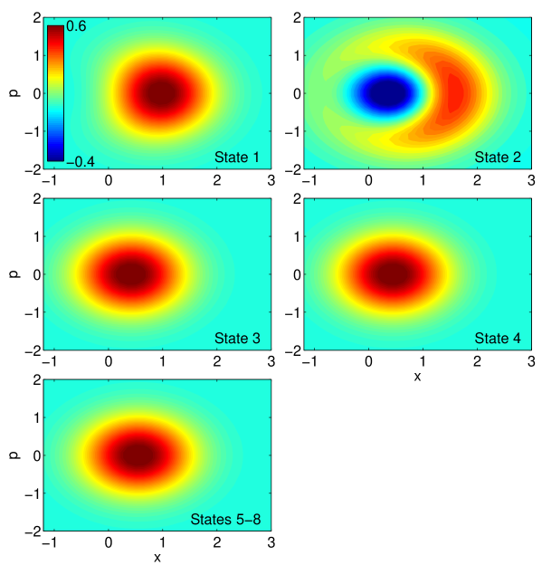
Figure 5: (Color online) Contour plots of Wigner functions for possible output states when the initial field is a coherent field with $|\alpha|=0.5$ and the beam splitter reflectivity is $r=0.4$.

The amplitude expectation values in Table 1 showed that the amplitude of the coherent output states 5–8 $|\langle\hat{a}\rangle|=0.385$ is clearly smaller than the amplitude of the initial field $|\alpha|=0.5$. This follows from the relatively large reflectivity of $r=0.4$. For a smaller reflectivity of $r=0.1$, the amplitude expectation value for the exactly coherent output states is $|\langle\hat{a}\rangle|=0.493$, which is much closer to the initial field amplitude. Since this output is also the most probable output and, in the case of small reflectivities, it is a nearly unchanged coherent state one could also try to repeat the amplification process in order to increase the probability of successful amplification. However, experimental realization of the repeated amplification setup would be challenging.

In principle, both the conventional noiseless amplification setups using single photon sources and the proposed setup relying purely on field fluctuations are based on the same basic concept. They use a device that constructs a complex superposition output state from the input and collapses the output state into the amplified target state as a result of certain measurements in the detectors of the device. This unavoidably leads to stochastic operation where the amplified state can be considered as a fluctuation in the output field, onto which the output state collapses. However, the proposed setup has also some subtle differences compared with the previously demonstrated noiseless amplification setups. Most importantly, the amplification in the proposed setup does not add any energy to the input signal and therefore nicely demonstrates that energy fluctuations in the original signal can be used as a stochastic energy source for the amplification.

3 Conclusions

In conclusion, we have studied noiseless amplification of coherent signals in a setup where all the energy added to the amplified signal originates from the fluctuations in the quantum field in a purely stochastic manner, i.e. the field is amplified even when no additional energy is added to the field from external sources in contrast to the previously reported noiseless amplifiers. We have discussed nonidealities in the setup and the effects and realizations of the QND detector needed in the setup. We have also shown that the probability of successful amplification can be maximized by finding optimal values for the beam splitter reflectivities depending on the desired effective gain. Our results show that the purely stochastic amplification scheme can amplify weak coherent fields with very good fidelities much like the conventional stochastic amplification setups relying on single photon sources.

References

- [1] Caves, C. M., “Quantum limits on noise in linear amplifiers,” Phys. Rev. D 26(8), 1817–1839 (1982).
- [2] Zavatta, A., Fiurasek, J., and Bellini, M., “A high-fidelity noiseless amplifier for quantum light states,” Nature Photonics 5, 52–56 (2011).
- [3] Ferreyrol, F., Barbieri, M., Blandino, R., Fossier, S., Tualle-Brouri, R., and Grangier, P., “Implementation of a nondeterministic optical noiseless amplifier,” Phys. Rev. Lett. 104, 123603 (Mar 2010).
- [4] Ferreyrol, F., Blandino, R., Barbieri, M., Tualle-Brouri, R., and Grangier, P., “Experimental realization of a nondeterministic optical noiseless amplifier,” Phys. Rev. A 83, 063801 (Jun 2011).
- [5] Barbieri, M., Ferreyrol, F., Blandino, R., Tualle-Brouri, R., and Grangier, P., “Nondeterministic noiseless amplification of optical signals: a review of recent experiments,” Laser Phys. Lett. 8(6), 411 (2011).
- [6] Marek, P. and Filip, R., “Coherent-state phase concentration by quantum probabilistic amplification,” Phys. Rev. A 81, 022302 (Feb 2010).
- [7] Häyrynen, T., Oksanen, J., and Tulkki, J., “Exact theory for photon subtraction for fields from quantum to classical limit,” Europhys. Lett. 87(4), 44002 (2009).
- [8] Häyrynen, T., Oksanen, J., and Tulkki, J., “Quantum trajectory model for photon detectors and optoelectronic devices,” Phys. Scr. T143, 014011 (2011).
- [9] Partanen, M., Häyrynen, T., Oksanen, J., and Tulkki, J., “Noiseless amplification of weak coherent fields exploiting energy fluctuations of the field,” Phys. Rev. A 86, 063804 (Dec 2012).
- [10] Josse, V., Sabuncu, M., Cerf, N. J., Leuchs, G., and Andersen, U. L., “Universal optical amplification without nonlinearity,” Phys. Rev. Lett. 96, 163602 (Apr 2006).
- [11] Grangier, P., Levenson, J. A., and Poizat, J.-P., “Quantum non-demolition measurements in optics,” Nature 396, 537–542 (1998).
- [12] Brune, M., Haroche, S., Lefevre, V., Raimond, J.-M., and Zagury, N., “Quantum nondemolition measurement of small photon numbers by rydberg-atom phase-sensitive detection,” Phys. Rev. Lett. 65(8), 976–979 (1990).
- [13] Milburn, G. J. and Walls, D. F., “State reduction in quantum-counting quantum nondemolition measurements,” Phys. Rev. A 30(1), 56–60 (1984).
- [14] Munro, W. J., Nemoto, K., Beausoleil, R. G., and Spiller, T. P., “High-efficiency quantum-nondemolition single-photon-number-resolving detector,” Phys. Rev. A 71, 033819 (Mar 2005).
- [15] Nogues, G., Rauschenbeutel, A., Osnaghi, S., Brune, M., Raimond, J. M., and Haroche, S., “Seeing a single photon without destroying it,” Nature 400, 239–242 (1999).
- [16] Guerlin, C., Bernu, J., Deleglise, S., Sayrin, C., Gleyzes, S., Kuhr, S., Brune, M., Raimond, J.-M., and Haroche, S., “Progressive fields-state collapse and quantum non-demolition photon counting,” Nature 448, 889–893 (2007).
- [17] Fiurášek, J., “Engineering quantum operations on traveling light beams by multiple photon addition and subtraction,” Phys. Rev. A 80, 053822 (Nov 2009).
- [18] Haroche, S. and Raimond, J.-M., [Exploring the Quantum ], Oxford University Press, Oxford (2006).
- [19] Brune, M., Bernu, J., Guerlin, C., Deléglise, S., Sayrin, C., Gleyzes, S., Kuhr, S., Dotsenko, I., Raimond, J. M., and Haroche, S., “Process tomography of field damping and measurement of fock state lifetimes by quantum nondemolition photon counting in a cavity,” Phys. Rev. Lett. 101, 240402 (Dec 2008).
- [20] Wang, H., Hofheinz, M., Ansmann, M., Bialczak, R. C., Lucero, E., Neeley, M., O’Connell, A. D., Sank, D., Wenner, J., Cleland, A. N., and Martinis, J. M., “Measurement of the decay of fock states in a superconducting quantum circuit,” Phys. Rev. Lett. 101, 240401 (Dec 2008).
- [21] Schleich, W. P., [Quantum optics in phase space ], Wiley-VCH, Berlin (2001).
- [22] Leonhardt, U., [Measuring the quantum state of light ], Cambridge University Press (1997).
- [23] Leonhardt, U., “Quantum physics of simple optical instruments,” Rep. Prog. Phys. 66, 1207–1249 (2003).
- [24] Gardiner, C. W. and Zoller, P., [Quantum noise ], Springer, Berlin (2004).
- [25] Lee, J., Kim, M. S., and Jeong, H., “Transfer of nonclassical features in quantum teleportation via a mixed quantum channel,” Phys. Rev. A 62, 032305 (Aug 2000).
- [26] Bazaraa, M. S., Sherali, H. F., and Shetty, C. M., [Nonlinear programming: theory and algorithms ], Wiley-Interscience, New Jersey, 3 ed. (2006).
- [27] Ralph, T. C. and Lund, A. P., “Nondeterministic noiseless linear amplification of quantum systems,” in [Quantum Communication Measurement and Computing Proceedings of 9th International Conference ], Lvovsky, A., ed., 155–160, AIP, New York (2008). arXiv:0809.0326.
- [28] Hadfield, R. H., “Single-photon detectors for optical quantum information applications,” Nature photonics 3, 696–705 (2009).
- [29] Miller, A. J., Nam, S. W., Martinis, J. M., and Sergienko, A. V., “State reduction in quantum-counting quantum nondemolition measurements,” Appl. Phys. Lett. 83, 791–793 (2003).
- [30] Waks, E., Inoue, K., Oliver, W. D., Diamanti, E., and Y.Yamamoto, “High efficiency photon-number detection for quantum information processing,” J. Select. Topics Quantum Electron. 9, 1502–1511 (2003).
- [31] Kim, M. S., “Recent developments in photon-level operations on travelling light fields,” J. Phys. B 41(13), 133001 (2008).