DNA viewed as an out-of-equilibrium structure

Abstract

Abstract: The complexity of the primary structure of human DNA is explored using methods from nonequilibrium statistical mechanics, dynamical systems theory and information theory. The use of chi-square tests shows that DNA cannot be described as a low order Markov chain of order up to $r=6$. Although detailed balance seems to hold at the level of purine-pyrimidine notation it fails when all four basepairs are considered, suggesting spatial asymmetry and irreversibility. Furthermore, the block entropy does not increase linearly with the block size, reflecting the long range nature of the correlations in the human genomic sequences. To probe locally the spatial structure of the chain we study the exit distances from a specific symbol, the distribution of recurrence distances and the Hurst exponent, all of which show power law tails and long range characteristics. These results suggest that human DNA can be viewed as a non-equilibrium structure maintained in its state through interactions with a constantly changing environment. Based solely on the exit distance distribution accounting for the nonequilibrium statistics and using the Monte Carlo rejection sampling method we construct a model DNA sequence. This method allows to keep all long range and short range statistical characteristics of the original sequence. The model sequence presents the same characteristic exponents as the natural DNA but fails to capture point-to-point details.

I Introduction

The DNA molecule is one of the most complex systems encountered in nature. By its intricate, aperiodic structure it constitutes an information source for the synthesis of the different entities and for the occurrence of the multitude of delicately balanced processes within living cells. Yet the connection between global DNA structure and its various functions remains to a large extent elusive, particularly in view of the coexistence of coding and non-coding regions and the realization of the important role of non-coding sequences in higher organisms alberts:2007 ; dunham:2012 ; arneodo:2011 .

One view of the DNA molecule frequently adopted in the literature is that of two nested non-overlapping symbolic sequences - the coding and non-coding regions - each of which is expressed in terms of four symbols/letters corresponding to the four bases A, C, G and T or in the contracted form of two symbols/letters, purines (A, G) and pyrimidines (T, C). The observed complexity of these nested sequences has been shaped during evolutionary time based on functional needs. Processes like single nucleotide mutations, insertion and deletion of segments, multiple repetitions of elements acting simultaneously over different length and time scales have shaped the complexity of current day genomes producing intriguing statistical properties arneodo:2011 ; roman:1998 ; messer:2007 ; carpena:2011 ; polak:2009 ; oliver:2008 . In this latter setting early investigations have shown that the succession of bases along coding regions in higher organisms presents short range correlations, whereas non-coding regions exhibit long-range correlations li:1992 ; stanley:1992 ; voss:1992 . For these organisms the coding segment length distribution has an exponentially falling tail whereas the non-coding segment one falls off as a power law almirantis:2001 ; oikonomou:2007 .

In the present work the structure of DNA, viewed as a symbolic sequence, is analyzed from the standpoint of nonequilibrium statistical mechanics, dynamical systems theory and information theory. A first question raised concerns spatial asymmetry along the sequence, its signatures and its role in information processing. A second question pertains to the identification and analysis of global indicators of the underlying complexity, beyond the linear correlations usually considered in the literature. To arrive at a quantitative formulation of these questions we view a DNA chain as the realization of a stationary stochastic process, i.e., a process where the probabilities $p_{i}$ of the different states/symbols attain rapidly limiting values as the sample size is increased, in which the role of the time step in the traditional setting is played by the “spatial” shift by one unit in sequence space.

The data along with the results of a preliminary statistical analysis are compiled in Sec. II. Section III is devoted to a Markov chain analysis, leading to the conclusion that the data cannot be fitted by a Markov chain of order up to 6. The issue of spatial asymmetry is addressed in Sec. IV in which probability fluxes are evaluated and shown to be different from zero, reflecting the breakdown of (generalized) detailed balance type conditions. In Sec. V this analysis is complemented by the evaluation of a series of entropy and information-like quantities, leading to interesting characterizations of the “dynamical” complexity as one advances along the original chain and along its reverse and of the information transfer between different parts of the chain. Exit distance and recurrence distance distributions, two global complexity indicators of special significance are computed from the data and analyzed in Sec. VI. The existence of long tails in the distributions and of long-range correlations in the associated lengths is established and confirmed further by the evaluation of Hurst exponents. Building on this information a construction algorithm of a “model DNA” possessing the same statistical properties as the natural one, free of extra assumptions, is outlined in Sec. VII. Different criteria for comparing model and natural DNA’s are also developed. The main conclusions are summarized in Sec. VIII.

II Data and statistical analysis

For the needs of our analysis we have employed the genomic data from two large human chromosomes (10 and 14) and two of the smaller ones (20 and 22). In the sequel we frequently use as working data set a long contig in Chromosome 20 of the Homo Sapiens genome. This genomic contig is the locus N1_011387 (primary assembly) and contains 26259569 base pairs (bps), while the entire Chromosome 20 contains $\sim 63\times 10^{6}$ bps. This contig is a DNA entity long enough to ensure good statistics, when addressing both the short and long range spatial properties. Moreover it is representative of the entire DNA molecule, since it contains both coding and non-coding sequences and other functional elements in similar densities as for all other human chromosomes. In particular, the nucleotide frequencies for the contig are: $p_{A}=0.289341,p_{C}=0.208691,p_{G}=0.209448$ and $p_{T}=0.292519$. Occasionally, unknown bps denoted by $N$ which still resist in todays sequencing techniques, are found in genomes. The $N$-percentage is very small and does not contribute significantly to the statistics. We can then choose either to eliminate all $N$’s or to replace them randomly with one of the other four $\{A,C,G,T\}$. For both choices the presented results are indistinguishable, up to insignificant statistical errors. Very similar nucleotide frequencies are found in the other human chromosomes. The frequency of the four base pairs is not constant throughout the genome but varies along the sequences depending on evolutionary factors and on the presence (or absence) of functional units. For example the presence of the complex $CpG$ is associated with the presence of isochores, DNA regions with high density of gene-coding regions. By coarse graining the alphabet at the PU-PY level, the latter frequencies become very close: $p_{PU}=0.498788$ and $p_{PY}=0.501210$. Thus, information on possible presence of isochores faints. Alternatively, by refining the alphabet, for example by considering explicitly the frequencies of doublets, triplets etc., information on finer and finer scales emerge, which cannot be adherent from superpositions of previous levels of observation. This is one of the main elements which leads one to characterize this molecules as complex, since different levels of complexity appear when varying the scale of observation.

For conciseness, we denote from now on purines and pyrimidines as states 1 and 2 respectively in the two-letter alphabet and $A,C,G,T$ as states 1,2,3,4 respectively in the four-letter alphabet. In Table 1 the two-letter and four-letter conditional probabilities

$$w_{ij}=W(i|j)=\frac{Prob(j,i)}{Prob(j)}$$ (1)

obtained by counting the frequencies of adjacent bps $i$ and $j$ averaged over the entire sequence are provided. Whereas $W$ in the two-letter case is nearly symmetric, it is markedly asymmetric in the four-letter case. In particular, $w_{32}$, the probability of encountering $G$ after $C$ is noticeably smaller than the others. This difference is well known in the biology literature and is attributed to the specific regulatory function of the $CpG$-complex in the human genome, being an essential structural element of the promoters. In spite of such differences all $w_{ij}$’s keep statistically significant values, suggesting that the process underlying the entire structure is ergodic. Higher order probabilities are obtained in a similar way (available upon request).

Two-letter alphabet	$w_{11}=0.559964$	$w_{12}=0.440037$	$w_{21}=0.437910$	$w_{22}=0.562090$
Four-letter alphabet	$w_{11}=0.324143$	$w_{12}=0.173548$	$w_{13}=0.245801$	$w_{14}=0.256508$
	$w_{21}=0.3533467$	$w_{22}=0.259233$	$w_{23}=4.575338E-002$	$w_{24}=0.341667$
	$w_{31}=0.2869938$	$w_{32}=0.210515$	$w_{33}=0.259181$	$w_{34}=0.243310$
	$w_{41}=0.2109355$	$w_{42}=0.206090$	$w_{43}=0.254663$	$w_{44}=0.328311$

Table 1: Conditional probabilities $w_{ij}$ as obtained from the DNA data.

III Markov chain analysis

In the preceding section we have drawn inferences about probabilities of various orders from a long, unbroken data set. These data are viewed as defining the states of an underlying system at points $n$ along the sequence, the succession of which is supposed to be governed by a set of probability laws. The first question that comes then to the mind is whether these laws can be expressed for all practical purposes in the form of a low order Markov chain.

A stochastic process $\{i_{n}\}$ is a Markov chain of order $s$ if the conditional probability

$$W\left(i_{n}|i_{1},i_{2},\cdots i_{n-1}\right)=\frac{Prob\left(i_{1},i_{2},\cdots i_{n}\right)}{Prob\left(i_{1},i_{2},\cdots i_{n-1}\right)}$$ (2)

is independent of $i_{m}$ for $m<n-s$. As stated in Sec. II it is understood throughout that all these probabilities are considered as stationary, in the sense of being independent of $n$. The simplest setting is that of a first order Markov chain, $s=1$. Suppose that the conditional probability matrix $W(i|j)=w_{ij}$ has been evaluated from some model. Estimating the singlet and doublet frequencies $np_{i}$ and $np_{ij}$ from the data by different independent counts, leads then one to test the legitimacy of the model as a first order Markov chain on the basis of the smallness of the differences $p_{ij}-p_{j}w_{ij}$. A fundamental result in this context is that the random vector

$$(np_{ij}-np_{j}w_{ij})/(np_{j})^{1/2}$$

converges to the normal distribution with covariance matrix determined by $w_{ij}$. Keeping in mind the independence of the different samples, it follows billingsley:1961 that the sum

$$\sum_{ij}\frac{(np_{ij}-np_{j}w_{ij})^{2}}{(np_{j}w_{ij})}$$ (3)

obeys asymptotically to the chi-square distribution. This opens the way to testing the order of the Markov chain within a certain confidence interval by chi-square type tests. These results can be extended rather straightforward to higher order Markov chains.

In many cases - including the problem addressed in this work - one disposes of no reliable model for estimating, a priori, the conditional probabilities $w_{ij}$. The question thus arises whether chi-square type tests for the order of the Markov chain can still be conducted on the sole basis of the data. As suggested in refs. hoel:1954 ; lowry:1968 ; avery:1999 the answer is in the affirmative provided that the following chi-square tests are used for the hypothesis that the chain is of the order $r$

$$\chi^{2}=\sum_{i_{1},i_{2}\cdots i_{s}}\frac{p_{i_{1},i_{2}\cdots i_{s}}-p_{i_{1},i_{2}\cdots i_{s-1}}W(i_{s}|i_{s-r}\cdots i_{s-1})}{p_{i_{1},i_{2}\cdots i_{s-1}}W(i_{s}|i_{s-r}\cdots i_{s-1})}$$ (4)

where the $W$’s are estimated from the data as ratios of frequencies of $i_{1},i_{2}\cdots i_{s-1}$ and $i_{1},i_{2}\cdots i_{s}$, $s$ being the maximum order considered.

To apply this test to our data we need to prescribe a confidence interval, which we have chosen to be 5%, and compare the corresponding $\chi^{2}$ value as given in the Tables to the value (4) obtained from the data. This requires specifying each time the number of degrees of freedom, which is related to $s,r$ and the number of states $N$ by

$$\text{DOF = Number of degrees of freedom =}N^{s}-N^{s-1}-(N^{r}-N^{r-1})$$ (5)

The order of the process is then estimated to be the smallest value of $r$ which produces a nonsignificant test statistics papapetrou:2013 ; menendez:2011 .

Orders compared	DOF	$\chi^{2}$-value (4)	$\chi^{2}$-value at 5% level
0 1	1	$0.391189\times 10^{6}$	3.84
1 2	2	$0.936032\times 10^{5}$	5.99
2 3	4	$0.840413\times 10^{4}$	7.81
3 4	8	$0.244684\times 10^{5}$	9.48
4 5	16	$0.341158\times 10^{5}$	11.07

Table 2: $\chi^{2}$-test (4) for the DNA data in the two-letter alphabet.

Orders compared	DOF	$\chi^{2}$-value (3.3)	$\chi^{2}$-value at 5% level
0 1	9	$0.143217\times 10^{7}$	17
1 2	36	$0.361137\times 10^{6}$	51
2 3	144	$0.165965\times 10^{6}$	150
3 4	576	$0.227638\times 10^{6}$	633
4 5	2304	$0.322366\times 10^{6}$	2417

Table 3: $\chi^{2}$-test (4) for the DNA data in the four-letter alphabet.

Tables 2 and 3 summarise the results from our data obtained using the chi-square test for the two- and the four-letter alphabets, respectively. In all cases tested the $\chi^{2}$ values obtained by applying (4) to the data turn out to be much larger than the confidence level ones for processes of order up to 6. In other words, the DNA data cannot be fitted by a low order Markov chain. For comparison, by simulating a first order Markov chain having the same $p_{i}$’s and $w_{ij}$’s as the data and by applying the test leads to a value of $0.182155\times 10^{6}$ for the first row of Table 2 and subsequently for the second raw to a value $0.392362\times 10^{1}$, smaller than the $\chi^{2}$ value of 5.99 at 5% level.

IV Spatial asymmetry and probability fluxes

The failure of the Markov property established in the preceding section leads us to search for alternative ways to characterize DNA viewed as a symbolic sequence, or alternatively, as a text written in the four-letter alphabet provided by the four nucleotides or in the restricted two-letter alphabet of purines and pyrimidines. A common syndrome of all languages is irreversibility in the form of “spatial” asymmetry, i.e., reading a text written in the language from, say, left to right produces a different result from reading it from right to left. In DNA sequences such spatial asymmetries may be expected due to the extensive presence of repetitive elements and to large scale patchiness polak:2009 ; oliver:2008 . In this section we address the issue of irreversibility and asymmetry for the DNA on the basis of data summarized in Sec. II.

At the microscopic level of description irreversibility and asymmetry are associated with the breakdown of the property of detailed balance, i.e., that in a given system the probability of an event leading from an initial state $i$ to a final state $j$ is counteracted by the probability of the reverse event leading from state $j$ to state $i$. This implies, in turn, the presence of a global constraint keeping the system out of the state of thermodynamic equilibrium. Transposed from the time domain to the one of the DNA symbolic sequence as it unfolds in space the simplest expression of this property amounts to the joint probability of two states $i$ and $j$ in adjacent positions $n$ and $n+1$ along the chain satisfying the “space reversal relation”:

$$p(i,n;j,n+1)=p(j,n;i,n+1)\hskip 142.26378pt$$ (6a)

or using the definition of conditional probabilities,

$$w_{ji}p_{i}=w_{ij}p_{j}\hskip 170.71652pt$$ (6b)

Here $i,j$ run from 1 to 4 in the case of the four-letter alphabet defined by the nucleotides and from 1 to 2 for the two-letter purine-pyrimidine alphabet. Alternatively, the probability flux $J^{(2)}_{ij}$

$$J^{(2)}_{ij}=w_{ji}p_{i}-w_{ij}p_{j}$$ (7)

vanishes if the detailed balance condition is satisfied. In a similar vein, higher order space reversal conditions involving more than two sites can be introduced, e.g.

$$P(i,n;j,n+1;k,n+2)=p(k,n;j,n+1;i,n+2)\hskip 113.81102pt$$ (8a)

or equivalently,

$$w_{kji}p_{ij}-w_{ijk}p_{kj}=p_{i}w_{ji}w_{kji}-p_{k}w_{jk}w_{ijk}=0\hskip 142.26378pt$$ (8b)

expressing the vanishing of the probability flux

$$J^{(3)}_{ijk}=w_{kji}p_{ij}-w_{ijk}p_{kj}$$ (9)

Notice that for an alphabet of more than two letters there are more than one probability fluxes and more than one detailed balance conditions. For instance in the four-letter alphabet there are six fluxes $J^{(2)}_{ij}$. If the process were first order Markov, these fluxes would be related by the stationarity condition:

$$p_{j}=\sum_{i}w_{ji}p_{i}$$

or, using the normalisation property $\sum_{i}w_{ij}=1$ ,

$$\sum_{i}\left(w_{ji}p_{i}-w_{ij}p_{j}\right)=\sum_{i}J^{(2)}_{ij}=0$$ (10)

There would then be only three independent fluxes, say $J^{(2)}_{12},J^{(2)}_{13}$ and $J^{(2)}_{23}$. One may also define composite fluxes, e.g. the flux from state 1 to the pyrimidines,

$$J_{1,PY}=\left(w_{21}p_{1}-w_{12}p_{2}\right)+\left(w_{41}p_{1}-w_{14}p_{4}\right)=J^{(2)}_{12}+J^{(2)}_{14}$$ (11)

and the purine-pyrimidine flux as

$$J_{PU,PY} =J^{(2)}_{12}+J^{(2)}_{14}+J^{(2)}_{32}+J^{(2)}_{34}$$

$$=J_{1,PY}+J_{3,PY}$$ (12)

The latter would be strictly zero had the process been a first order Markov.

We now proceed to the evaluation of the probability fluxes from the data and to the testing of the detailed balance condition. Table 4 summarises the main result for fluxes $J^{(2)}$ and $J^{(3)}$ in the case of the two-letter alphabet. As can be seen, the fluxes are very small. Actually they are indistinguishable from those obtained from a random sequence of the same length and with probabilities $p_{i}$ fitted from the data (not shown). Detailed balance holds therefore true in this case, or, to put it differently, there is no overall spatial asymmetry and irreversibility. This is compatible with the symmetry of the associated conditional probability matrix pointed out in Sec. II.

$J^{(2)}$
12	$2.9802\times 10^{-8}$
$J^{(3)}$
112	$5.2154\times 10^{-8}$
212	$3.7252\times 10^{-8}$

Table 4: Probability fluxes $J^{(2)}$ and $J^{(3)}$ in the two-letter alphabet

Table 5 summarises the results for $J^{(2)}$ and $J^{(3)}$ in the case of the four-letter alphabet. The results are now definitely significant, much larger than those obtained from a random sequence. We conclude that detailed balance does not hold here, in other words, there is an overall irreversibility in the form of spatial asymmetry. Following the analogy with the theory of stochastic processes and nonequilibrium statistical mechanics, one would be tempted to state that the structure as a whole can be viewed as a system subjected to constraints maintaining it far from the state of thermodynamic equilibrium. This may, at a first sight, sound in contradiction with the usual view of DNA as a stable molecule in thermodynamic equilibrium with its environment. But the contradiction is only apparent inasmuch as complex matter in general, and DNA in particular as we observe it today, is to be viewed as the outcome of a primordial nonequilibrium evolutionary process that was eventually stabilised in a “fossil” form as a result of the action of local short-ranged intermolecular interactions. Otherwise, the waiting time to see this event happen spontaneously would be exceedingly large owing to the combined effects of detailed balance and of the explosion of the number of possible combinations of the constituting subunits among which only a small subset would posses the desired biological functions nicolis:1989 ; nicolis:2012 ; frisch:1984 .

$J^{(2)}$
12	$-2.3525\times 10^{-2}$
14	$1.2515\times 10^{-2}$
32	$3.4543\times 10^{-2}$
34	$-2.3533\times 10^{-2}$

$J^{(3)}$
123	$1.1347\times 10^{-2}$
124	$7.7443\times 10^{-3}$
134	$6.6033\times 10^{-4}$
213	$-1.2467\times 10^{-2}$
214	$-3.7790\times 10^{-3}$
234	$1.2393\times 10^{-2}$
312	$1.2358\times 10^{-2}$
314	$-3.6969\times 10^{-3}$
412	$7.8714\times 10^{-4}$
413	$7.5745\times 10^{-3}$

Table 5: Probability fluxes $J^{(2)}$ and $J^{(3)}$ in the four-letter alphabet

V Entropy analysis and information transfer

In this section we introduce and analyse a set of quantities aiming to characterise the complexity of the DNA symbolic sequence, while accounting for its central role as information source ebeling:1991 ; nicolisjs:1991 ; roman:1996 as well as for the spatial asymmetry and irreversibility established in the preceding section. The simplest quantity in this family is the information (Shannon) entropy:

$$S_{I}=-\sum_{i}p_{i}\ln p_{i}$$ (13)

describing the amount of choice exercised by the information source and the associated uncertainly of the message recipient. By its static character this quantity does not provide insights on the overall structure of the sequence. To handle this aspect we divide the sequence into blocks of symbols $i_{1},i_{2}\cdots i_{n}$ of length $n$ and extend Eq. (13), which defines essentially the entropy per symbol, to the entropy per block of symbols over a window of length $n$:

$$S_{n}=-\sum_{i_{1},i_{2},\cdots i_{n}}P(i_{1},i_{2},\cdots i_{n})\ln P(i_{1},i_{2},\cdots i_{n})$$ (14)

where the sum runs over all sequences compatible with the underlying rules.

Now suppose that the source has sent a message in the form of a particular $n$-sequence. What is the probability that the next symbol be $i_{n+1}$? Clearly we are dealing here with a conditional event. The entropy excess associated with the addition of an extra symbol to the right of the $n-$block (“word”) is then nicolis:2012 ; ebeling:1991 :

$$h_{n}=-\sum_{i_{1},i_{2},\cdots i_{n},i_{n+1}}P(i_{1},i_{2},\cdots i_{n})W(i_{n+1}|i_{1},i_{2},\cdots i_{n})\ln W(i_{n+1}|i_{1},i_{2},\cdots i_{n})$$ (15)

The first nontrivial value $h$ of $h_{n}$ describes the amount of information obtained when one moves along the chain one step ahead of the initial state $i_{1}$,

$$h=h_{1}=-\sum_{i,j}p_{i}w_{ji}\ln w_{ji}$$ (16)

Actually, $h_{n}$ would be $n-$independent and equal to $h$ had the sequence been compatible with the Markov property, which, as shown in Sec. III, is not the case. In spite of this failure, (16) keeps its significance whatever the nature of the process and will be referred to, in the sequel, as the Kolmogorov-Sinai (KS) entropy. To capture the asymmetry property analysed in Sec. IV it is also useful to introduce the reverse process in which the order of the states visited is running backwards, and to define the associated KS entropy as

$$h^{R}=-\sum_{i,j}p_{i}w_{ji}\ln w_{ij}$$ (17)

One can easily check that if the Markov property holds $h^{R}$ is larger than or equal to $h$. Indeed,

$$\sigma_{I}=h^{R}-h=\sum_{ij}p_{i}w_{ji}\ln\frac{w_{ji}}{w_{ij}}$$ (18)

or using the normalisation and stationarity properties discussed in Sec. IV nicolis:2012 ; gaspard:2004 ; luo:1984 ; andrieux:2008 ,

$$\sigma_{I}=h^{R}-h=\frac{1}{2}\sum_{ij}\left(w_{ji}p_{i}-w_{ij}p_{j}\right)\ln\frac{w_{ji}p_{i}}{w_{ij}p_{j}}\geq 0$$ (19)

We can express this property by the statement that the direct sequence is more ordered than the reverse one as long as the probability flux $J^{(2)}_{ij}$ (Eq. (7)) does not vanish, i.e., as long as detailed balance does not hold. For this reason we will refer to $\sigma_{I}$, which can be regarded as a distance from the regime of detailed balance, as the information entropy production. Conversely, in absence of the Markov property but knowing that $J^{(2)}_{ij}$ is different from zero, one may wonder whether $h^{R}$ is still larger than $h$. As we see shortly, this is indeed the case for the DNA sequence in the four-letter alphabet.

Let now $n$ be gradually increased. As stated earlier in a Markov process $h$ would remain constant, entailing that $S_{n}$ would increase linearly in $n$. Figure 1 depicts the dependence of $S_{n}$ and $h_{n}$ as defined from Eqs. (14)-(15) for the DNA data of Sec. II. As can be seen the $S_{n}$ versus $n$ dependence is not strictly linear. $h_{n}$ varies thus (weakly but systematically) with $n$ from a value 1.339 for $n=1$ to 1.273 for $n=8$, in the case of the four-letter alphabet (solid lines in Fig. 1). This is in accord with the conclusion drawn in Sec. IV on the non -Markovian character of the sequence and suggests the presence of long-range correlations (see also Sec. VI below).

As expected the value $h_{1}$ reported above is identical to the value $h$ as computed directly from the data. Table 6 summarises the results of evaluation of $h$, $h^{R}$ and $\sigma_{I}$ using Eqs. (16)-(18), for the four-letter alphabet. For comparison the corresponding values from a random sequence of the same length are also given. In this case, as expected $h$ and $h^{R}$ are both equal to the maximum entropy, $h=h^{R}=\ln 4$, of the sequence and $\sigma_{I}=0$.

	$h$	$h^{R}$	$\sigma_{I}$
DNA Data	1.339	1.416	0.077
Random sequence	1.373	1.373	4$\times 10^{-7}$

Table 6: Kolmogorov entropy of the direct and reverse sequence and information entropy production as computed from the DNA data.                                    

The evaluation of the quantities in Table 6 for the DNA sequence in the two-letter alphabet leads to the quite different conclusion that $h\sim h^{R}=0.686$ and thus $\sigma_{I}\approx 0$, the corresponding $h-$value for the random sequence being $h\sim\ln 2=0.693$. On the other hand $S_{n}$ and $h_{n}$ still depend on $n$ in a non-trivial way, see dashed lines in Fig. 1. The signature of the non-Markovian character at the level of the entropy quantities therefore persists in the two-letter alphabet case.

On the basis of the above comparison between the two alphabets and between the DNA data and those associated to the random sequence, one is tempted to conclude that revealing the asymmetry of the DNA sequence in the four-letter alphabet - as established already in Sec. IV - has also some interesting signatures at the level of information processing: Information is being produced (in the sense $\sigma_{I}>0$) as long as one advances along a preferred direction in sequence space, and this requires reading the “text” in a four-letter alphabet.

Figure 1: a) Information entropy $S_{n}$ for blocks of size $n$ for the DNA data in the four- and two-letter alphabets; b) Entropy excess $h_{n}$ for block of size $n$ for the DNA data in the four- and the two-letter alphabets.                                   

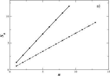
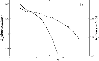
An alternative view of the DNA sequence in connection with both the presence of correlations and information processing is to consider two segments - typically of the same length - view the leftmost segment (say $x$) as the “source” and the second one (say $y$), as the “receiver” and evaluate the information transfer from $x$ to $y$. We define this quantity as nicolisjs:1986 :

$$I_{x\to y}=\sum_{i,j}P(x_{i},y_{j})\ln\frac{P(x_{i},y_{j})}{P(x_{i})P(y_{j})}.$$ (20)

We notice that

$$I_{x\to y}=S_{I}(y)+\sum_{i,j}P(x_{i},y_{j})\ln W(y_{j}|x_{i}).$$

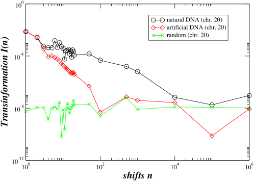
Furthermore, if $x$ and $y$ are two adjacent sites of the sequence the second term, which represents the conditional entropy of $y$ given the state of $x$, reduces to the KS entropy (Eq. (16)). In the following analysis a sequence is compared with its shifts. For a specific shift of $n$ sites, the information transfer represents then the capacity between adjacent symbols to interact down the sequence. The upper line in Fig. 2 depicts the dependence of $I_{x\to y}$ on $n$ for two sequences of the same length: the chromosome 20, working contig N1_011387 (in two-letter representation) and its shift by 1,2, $\cdots$ up to $10^{5}$ symbols. The last excess $n$ symbols in the comparison can either be reinjected at the beginning of the sequence, or they can be neglected without changing significantly the resulting $I$ values. For comparison, the lower line (with crosses) stands for the results obtained from random sequences of the same length and bps frequencies. The intermediate line (with diamonds) is associated with the model which will be discussed in Sec. VII. As can be seen from the figure the information transfer as extracted from the DNA data remains higher with respect to the case of a random sequence for shifts up to 100, suggesting, once again, the presence of correlations and information transfer between successive bps up to the order of $\sim 100$. At the level of functionality, this nontrivial information transfer may refer to cooperations between successive units related to the presence of codons in the coding regions and to the multiple presence of poly-A’s, to frequent appearance of repetitive elements, to the regulatory elements, to the promoters and to other functional elements in the non-coding parts kalkatawi:2012 ; lustig:1984 .

Figure 2: (Colour online) Information transfer $I(n)$ between a sequence and its shift by $n$ symbols versus $n$. Line with circles depicts the DNA sequence, line with crosses a random sequence and line with diamonds a model-generated sequence (Sec. VI).

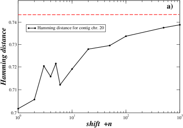
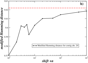
A different view of the presence of correlations in information transfer between two symbol sequences is provided by their Hamming distance, which determines the number of positions at which the corresponding symbols are different or counts the number of substitutions required to change one sequence into the other. The classical Hamming distance $H_{1-2}$ between the two symbol sequences $S1$ and $S2$, as defined by R. Hamming in 1950 for error detection, is hamming:1950 :

$$\begin{array}[]{l l}H_{1-2}=\sum_{i}d_{i},&\quad\text{where }\\ d_{i}=\left\{\begin{array}[]{l l}0&\quad\text{if $S1(i)=S2(i)$}\\ +1&\quad\text{if $S1(i)\not=S2(i)$}\end{array}\right.\end{array}$$ (21)

We shall also use a modified Hamming distance $HM_{1-2}$ between $S1$ and $S2$, defined as

$$\begin{array}[]{l l}HM_{1-2}=\sum_{i}d_{i},&\text{where}\\ d_{i}=\left\{\begin{array}[]{l l}0&\quad\text{if $S1(i)=S2(i)$}\\ +0.5&\quad\text{if $S1(i)$ and $S2(i)$ are both purines}\\ +0.5&\quad\text{if $S1(i)$ and $S2(i)$ are both pyrimidines}\\ +1&\quad\text{otherwise}\end{array}\right.\end{array}$$ (22)

which considers the purine-purine variation as less important than the purine-pyrimidine one and penalises by 0.5 the $PU-PU$ discrepancy and by 1 the $PU-PY$ difference.

In the case of the original Hamming distance, the $H-$distance between the contig sequence and a random one with the same symbol frequencies is $H(contig-random)=0.74331$. Note that if the 4 symbol frequencies were equal the value would be $12/16=0.75$. The $H-$value between two random sequences are of the same order $H(random1-random2)=0.74329$. The $H-$value between the contig sequence and its shifts shows, on the contrary, interesting correlations similar to the ones demonstrated by the information transfer, see Fig. 3a.

In the case of the modified Hamming distance, the $HM-$distance between the contig sequence and a random one with the same symbol frequencies is $HM(contig-random)=0.6216$. The $H-$value between two random sequences are of the same order $HM(random1-random2)=0.6220$. Again, the $HM-$value between the contig sequence and its shifts shows interesting correlations, similar to the ones demonstrated by the information transfer and the original $H$-distance, see Fig. 3b.

Figures 3a,b demonstrate overall that there is a non-trivial information flow between each bps and its neighbours, while this information decreases as the bps become more and more distant on the chain.

Figure 3: (Colour online) a) The classical Hamming distance $H_{1-2}$ between the contig sequence and its shifts. The red dashed line denotes the $H-$value between two random sequences with the same symbol frequencies. b) The modified Hamming distance $HM_{1-2}$ between the contig sequence and its shifts. The red dashed line denotes the $HM-$value between two random sequences with the same symbol frequencies. All sequences are represented in the four-letter alphabet.

VI Exit and recurrence distance distributions

So far we have been concerned with global properties of the DNA sequences. In this section we introduce a new set of quantities which allow probing features associated with the local structure. One example of special importance is the appearance of clusters in which a given symbol - or a given subsequence of symbols - is repeated for a certain number of steps, beyond which a transition to different symbols or subsequences is taking place.

To capture such features we introduce the exit distance distribution, a concept analogous to the exit time distribution familiar from the theory of stochastic processes feller:1968 ; gardiner:1983 . Specifically, starting with a certain state/symbol $j$, we ask for the probability $q_{j,n}$ that an escape from it occurs at the n-th step as one moves along the sequence bala:1997 :

$$q_{j,n}=Prob(j,1:\overline{j},n)/Prob(j,1)$$ (23)

where $\overline{j}$ denotes the set of all allowed states with the exception of $j$.

Closely related to the above is the recurrence distance distribution in which starting again with a state $j$ we ask what is the probability $F_{j,n}$ to encounter this state again $n$ steps down the sequence, with the understanding that the sites between 1 and $n$ are found in states $\overline{j}$, other than $j$:

$$F_{j,n}=Prob(j,1;\overline{j},2;\cdots;j,n)/Prob(j,1)$$ (24)

For a first order Markov process both $q_{j,n}$ and $F_{j,n}$ can be evaluated explicitly on the sole basis of the conditional probability matrix $W=\{w_{ij}\}$. Specifically,

$$q_{j,n}=(w_{jj})^{n-1}-(w_{jj})^{n}$$ (25)

and $F_{j,n}$ is expressed in terms of its generating function $\tilde{F}_{j}(s)$ as

$$\tilde{F}_{j}(s)=\left[sW(I-sW)\right]^{-1}$$ (26)

where $I$ is the unit matrix. As a corollary, both $q_{j,n}$ and $F_{j,n}$ are superpositions of exponentials in $n$ and thus fall off exponentially for large $n$.

Equations (25)-(26) can be extended rather straightforwardly to the case of a second-order Markov process. The calculations are more involved, but the property of exponential decay for large $n$ is again found to hold here.

We now proceed to the evaluation of these distributions from the DNA contig data in Sec. II, starting with $q_{j,n}$. For this purpose the data is being read along the direct sequence. Whenever a state $i$ is first spotted the origin of coordinates is set on the corresponding site and the distance from the origin is recorded when a state different from $i$ first appears along the sequence. Counting all the distances recorded in this way for each of the states one arrives at the exit distance distribution. In Figs. 4a,b the distributions for state $C$ and for $PU$ in the case of the four- and the two-letter alphabets, respectively, are depicted. In both cases we observe the tendency for development of long tails (see also refs. masoliver:1986 ; altmann:2012 ). In particular in the case of the four-letter alphabet the state $C$ shows a linear region of low slope ($\sim-2$) in the intermediate scales which is soon covered by finite size effects. The tendency for development of long tails is better detected from comparison with the associated probability for a first order Markov process indicated in the figures by the dashed lines as obtained from a direct simulation of a Markov chain with conditional probabilities equal to those provided by the data. Interestingly, the exit distributions from states $A$ and $T$ and from states $C$ and $G$ are indistinguishable. Furthermore, the distribution of $A$ and $T$ is longer-ranged than the one of $C$ and $G$ (not shown), owing principally to the existence of poly(A) and poly(T) domains found in the human genome kalkatawi:2012 ; lustig:1984 .

Figure 4: (Colour online) Exit distance distributions: a) four-letter alphabet, $C-$state; b) two-letter alphabet, $PU-$state.                                                                                       

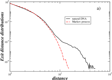
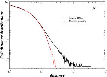
An alternative manifestation of the log-log structure depicted in Figs. 4a,b is that the individual exit distances display long-range correlations as illustrated in Fig. 5, curves a and b, for the cases of four and two symbols, with power law decaying exponents close to 1/3 and to 1/2, respectively.

Figure 5: (Colour online) Correlation function: four-letter alphabet (curve a) and two-letter alphabet (curve b).                                                             

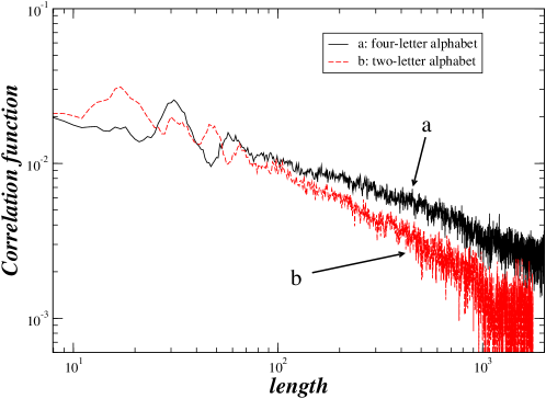
Table 7 summarises the mean and variances of the exit distances for the four- and for the two-symbol cases as compared to the corresponding quantities evaluated from the Markov chain simulation. We see that while the average values in the two cases are practically indistinguishable (and equal to the analytic results for a first order Markov chain, $(1-w_{ii})^{-1}$), the variances associated to the data are larger than the Markov ones. This reflects the delocalisation of the DNA exit distance distribution in the state space, a property due among other to the presence of repeats along the sequence.

		DNA Data		1st order Markov
		$<n>$	$<\delta n^{2}>$	$<n>$	$<\delta n^{2}>$
Two-letter alphabet	1	2.2725391	3.5143790	2.2719333	2.4828568
	2	2.2835724	3.7262988	2.2843783	2.5242081
Four-letter alphabet	1	1.4796035	0.9562388	1.4791129	0.7088170
	2	1.3499513	0.4599166	1.3502789	0.4731067
	3	1.3498576	0.4588480	1.3498057	0.4724476
	4	1.4887851	0.9832494	1.4887587	0.7272797

Table 7: Means and variances of exit distances for the DNA data and for a 1st order Markov chain.                                                             

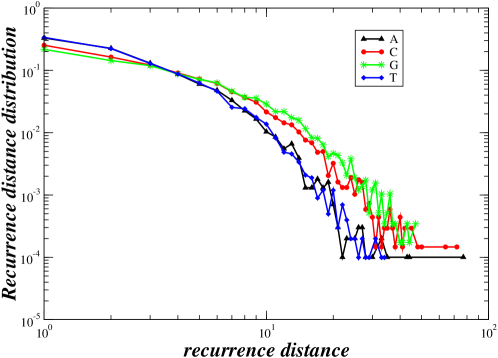
We turn next to the recurrence distribution $F_{j,n}$. We first observe that in the two-letter alphabet the recurrence distribution of one of the two states is fully determined by the exit distance distribution of the other state. We are thus again in the presence of long-ranged distributions and long range correlations of the individual recurrence distances, see Figs. 5 and the first two rows of Table 7. Coming to the four-letter alphabet, as for $q_{j,n}$, practically identical recurrence distributions for states $A$ and $T$ and for states $C$ and $G$ are observed, see Fig. 6. Both distributions are long ranged with the $A$ and $T$ falling off more slowly than for $C$ and $G$ for large $n$ (and a crossover between the two distributions at $n\sim 5$). Furthermore, compared to the corresponding exit distance distributions, they are more delocalised as illustrated by Table 8, to be compared with the last four rows of Table 7.

As was the case of Table 7 the averages $<n>$ are very close to those obtained by simulating a first order Markov chain with a conditional probability matrix provided by the data, as well as with the well known analytic result $<n>=1/p_{i}$.

	DNA Data		1st order Markov
	$<n>$	$<\delta n^{2}>$	$<n>$	$<\delta n^{2}>$
1	3.6221180	12.571706	3.6272037	9.004858
2	5.1011710	29.414993	5.1058583	20.609692
3	5.0786543	29.119154	5.0796456	20.368145
4	3.5896053	12.082341	3.5923173	8.781096

Table 8: Means and variances of recurrence distances for the DNA data and for a 1st order Markov chain.                                                                      

Figure 6: (Colour online) Recurrence distributions of the four symbols.

Closely related to recurrence is the concept of analogs, which finds its origin in the classification of atmospheric circulation patterns in meteorology. Translated in the language of the (coarse-grained) description of a symbolic sequence the issue is, to what extent there exist persistent patterns in different (distant) parts along the sequence, where symbols are found in a given prescribed order with an appreciable frequency nicolisc:1998 .

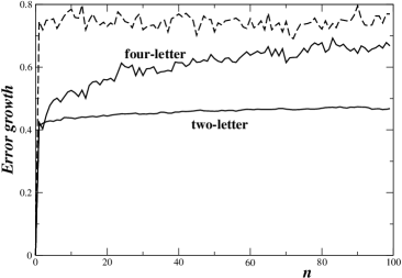
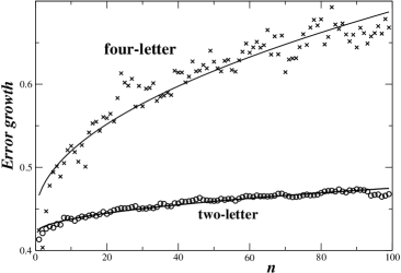
To address this question for the DNA symbolic sequence we consider all pairs of n-subsequences along the full sequence containing identical symbols in sites $1,\cdots$ up to $m$, and compute the “error” (in the sense of the Hamming distance, see Sec. V) as they start deviating from the $(m+1)$-st site and onwards. The result for the two and four-letter alphabets and for $n=100,\>\>m=8$ is depicted in Fig. 7a. The dashed lines in this figure correspond to a random sequence. As expected, beyond $n=8$ the symbols in the two members of the pair alternate indifferently between being identical (error 0) or being different (error 1), entailing that the error attains immediately a saturation value. The situation is very different for the DNA data, represented by the solid lines in Fig. 7a. Here a first stage of abrupt increase of the error is followed by a stage of very slow increase toward the saturation level, even though this level is not yet attained for $n$ up to 100. This indicates a persistence trend or, alternatively, the presence of long-range correlations and is further confirmed by the plot of Fig. 7b suggesting a power law dependence of the error on $n$ prior to the final decay to the saturation level with a power of the order of 0.5. This behavior can be viewed as the “spatial” analog of the error growth dynamics familiar from dynamical systems theory where, after an exponential stage (to be compared with the stage of fast growth in Fig. 7a), one observes a diffusive stage prior to the final stabilization to the saturation level.

Figure 7: a) Error growth functions for the two-letter alphabet and the four-letter alphabet; the dashed line represents a random sequence). b) Same as (a) with solid lines depicting nonlinear fit.

Within the set of quantities which probe the local structure of a sequence, the Hurst exponent $H$ expresses the tendency of the future values of a sequence to persist or increase on average, or to fluctuate between small and large values feder:1988 . In particular, for the range $0\leq H<0.5$ the sequence values tend to alternate, while for $0.5<H\leq 1$ they tend to persist or increase on average. The value 0.5 is a border case, where the values are either completely uncorrelated or their correlations decay exponentially fast to zero.

To apply the concept of the Hurst exponent in DNA sequences (or any symbol sequence in general) we map the nucleotides (symbols) to numbers. For the calculations we use the two-letter alphabet $PU-PY$ notation, to conform with the previous analysis on the exit distance distributions and the mapping takes the form:

$$PU\to 0$$

$$PY\to 1$$ (27)

Thus the symbol sequence turns into a corresponding numerical sequence, which carries all the information on the position of symbols. $H$ is then directly calculated from the numerical series and is a significant measure which expresses the tendency of symbols to repeat themselves (persistence) or to alternate (antipersistence) down the sequence.

The calculation of the Hurst exponent is based on the computation of the range $R(n)$ between the maximum and the minimum cumulative values as one advances along the numerical sequence of size $n$, for various values of $n$. Cumulative values are essential in the $H$ estimation because they keep track of the tendencies along the sequence. One then needs to rescale $R(n)$ by the standard deviation $S(n)$,

$$S(n)=\sqrt{\frac{1}{n}\sum_{i=1}^{n}(x_{i}-<x>)^{2}}$$ (28)

in order to obtain the rescaled range. Once the rescaled range $R(n)/S(n)$ is calculated it is averaged over many sequences (configurations) of the same length $n$.

$$E(n)=\langle\frac{R(n)}{S(n)}\rangle_{confs}$$ (29)

The Hurst exponent is then defined as

$$E(n)=c\cdot n^{H}$$ (30)

and is computed from the slope of $E(n)$ versus $n$ in a double logarithmic scale. When the sequence is characterised by fractality, with fractal dimension $D$, it can be shown that $H=2-D$, where $1<D<2$.

Figure 8: The rescale range $E(n)$ as a function of the sequence size $n$, for the calculation of the Hurst exponent $H$.                                                    

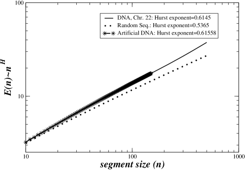
In Fig. 8 the rescaled ranges $E(n)$ are plotted as a function of $n$ for the working contig N_011387 of Chromosome 20 (solid line), the random sequence (dotted line) and the model DNA (stars) which will be discussed in the following section. The value calculated for the Hurst exponent is $H=0.6145$ and is clearly distinct from that of the random sequence with the same letter frequency as the data. Calculations of the Hurst exponent in other human contigs give very similar $H$-values. Values of $H>0.5$ indicate persistence of the same symbols along the sequence, or to put it differently, clustering of similar nucleotides. This effect is a cause of correlations and can reflect the well known existence of poly(A) and poly(T) (in the complementary chain) motifs in the primary genomic DNA sequences that give rise to the corresponding poly(A) signals in mRNA kalkatawi:2012 . Another source of the clustering of similar nucleotides is the Alu repeats hackenberg:2005 ; price:2004 in the human genome which are also known to be associated with poly(A) sequences lustig:1984 . In addition, non-coding gene-poor (desert) regions are known to be rich in A and T inducing clustering of these symbols, while CpG rich regions (isochores) are rich in genes and induce lower scale clustering li:2003 ; oliver:2002 ; luque:2005 ; bernaola:2004 ; arndt:2005 .

VII A model DNA

DNA, a complex multicomponent structure which has evolved during billions of years in close contact with an ever-changing environment, cannot be described or constructed based on a closed functional expression with a limited number of parameters. Statistical constructive methods or methods based on chaotic dynamics have been used since the early 1990 to create long nucleotide sequences with statistical properties mimicking those of specific DNA molecules stanley:1992 ; almirantis:2001 ; gutierez:2001 ; herzel:1995 ; provata:1999 ; allegrini:1995 ; beck-prov:2011 . All these attempts predict well some of the sequence properties but they fail in others and one needs to add an increasing number of parameters to probe into the structure’s local details, even from the statistical point of view. In the present section we propose a novel, global statistical construction method based on the exit distance distribution of the DNA sequence described in Sec. VI, to generate two- and four-letter sequences with statistical properties basically identical with the ones of the original DNA data.

The construction method is known as “Monte Carlo rejection sampling”, or simply rejection sampling, and dates back to J. von Neumann. Having calculated the exit distance distributions for the segments of all symbols in the natural DNA sequence, we use the rejection sampling method to create a statistically equivalent series. For simplicity, the method is described in the two-letter alphabet and is easily extendable to the four-letter one.

1. Define first the initial symbol as a $PU$ or $PY$, either randomly or as dictated by the contig sequence.

2. Select an integer random number between $\left[1,N_{PU}^{max}\right]$ or $\left[1,N_{PY}^{max}\right]$ depending on whether a $PU$ or a $PY$ segment is to be created. [$N_{PU}^{max}$ and $N_{PY}^{max}$ are the maximum numbers of juxtaposed $PU$’s or $PY$’s which have been observed in the natural contig]. Call the selected number $n$.

3. Chose a second random number $r\in\left[0,1\right]$ and compare it to the value of the exit distance distribution $q_{PU,n}$ or $q_{PY,n}$ depending on the current state on the chain.

4. If $r\leq q_{PU,n}$ (or $r\leq q_{PY,n}$) then the sequence is extended by $n$ units of $PU$ (or $PY$).

5. The algorithm returns to step 2 in order to make alternating additions of $PU$ and $PY$ clusters.

6. The algorithm stops when the size of the artificially constructed sequence is equal to the size of the natural DNA contig.

The artificial sequences created with the rejection sampling method are constructed to respect perfectly the exit distance distributions of the natural sequence. They possess all other statistical properties of the natural sequence as well, since the knowledge of the exit distance distribution alone is sufficient to carry out the construction. In particular, exit from a given state implies automatically entrance to the complementary state in the two-letter alphabet. The situation is different in the four-letter case. Here, one more assumption needs to be made regarding the alternation between the four symbols. Our procedure is based on the transition probabilities $w_{ij}$ between the different letters as were presented in Table 1 and implies thus the assumption that higher order transition probabilities are not accounted for at this stage.

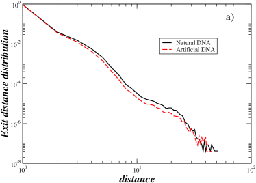
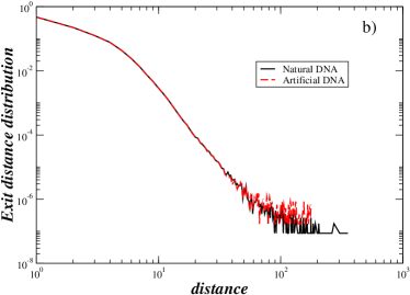
In Fig. 9 the exit distance distributions for the $A$ symbols (four-letter alphabet) and the $PU$ coarse grained symbol (two-letter alphabet) are shown, both for the original and the artificial model-based DNA sequence; similar plots are obtained for the other symbols. As one can see, the distributions are almost identical in the case of the two-letter alphabet, Fig. 9b, with small differences in the tails of the distribution attributed to the finite size of the sequences. The differences are non-trivial in the case of the four-letter alphabet, Fig. 9a, and this is attributed to the use of $w_{ij}$’s which account only for the pair correlations, while for the juxtaposition of segments of size $n$ higher order correlations (of range up to $n$) need to be taken into account.

Figure 9: (Colour online) Exit distance distributions for natural (solid black lines) and artificial DNA (red dashed line) : a) four-letter alphabet, $A$-symbol; b) two-letter alphabet, $PU$-symbol.                                                                                                                         

In Sec. V, Fig. 2, the information transfer $I$ between a sequence and its shifts was shown, both for the original and for the model-generated sequence. Both sequences show the same degree of information transfer in first and second neighbour positions. However, for more distant positions the information transfer in the model-generated sequence undergoes an abrupt decay as compared with the natural DNA sequence where the information transfer persists for hundreds of units. This difference reflects the functional role of natural DNA sequence, as opposed to the statistical character of the artificial DNA. The nucleotides in a natural sequence need to control the information about neighbouring positions, since what dictates their functionality is their precise (not statistical) juxtaposition. In particular, information flow in decades of bps relates to the turn of the helix, while information flow in a few hundreds of bps is plausible, since these are typical sizes for coding regions and for repetitive elements.

In a similar vein, the analog analysis shows that the error values as obtained from the model lie closer to the saturation level than those obtained from the natural DNA as depicted in Figs. 7. Interestingly, the Hamming and modified Hamming distances between the natural and the model sequences equal to 0.7444 and 0.6222, respectively and are close to the values associated with distances between random sequences.

Finally, in Sec. VI, Fig. 8, the Hurst exponent $H$ is depicted both for the natural (solid line) and for the model sequence (stars). By its nature $H$ is a nonlinear measure which takes into account all orders of correlations since it deals simultaneously with all segment sizes. As can be seen from the figure the curves $E(n)$ for the natural and the model sequence are practically indistinguishable and the values of $H$ are very close.

VIII Conclusions

In this study the structure of global human chromosomal sequences has been analyzed using ideas and tools from nonlinear dynamics, information and complexity theories and nonequilibrium statistical mechanics. We have shown that in the four-letter alphabet the sequence exhibits spatial asymmetry and suggested on these grounds that the DNA molecule can be viewed as an out-of-equilibrium structure. We have established a connection between these properties and the generation of long-range correlations and the processing of information along the sequence, using a series of entropy-like quantities. We have introduced the exit and recurrence distance distributions, two new indicators of the complexity underlying the sequence, whose evaluation revealed a number of interesting features of its global structure. Finally we have designed an algorithm generating sequences that share the statistical properties of natural DNA, local as well as global, on the sole basis of the exit distance distribution. The results reported pertain to human chromosome 20. Other chromosomes (10, 14 and 22) have been tested and shown to lead to similar conclusions.

The approach initiated in this work opens some interesting and worth-exploring perspectives. A first line of approach would be to apply the ideas of asymmetry, irreversibility and information processing considered here in a global perspective to particular DNA building blocks such as coding DNA, non-coding DNA, repeats, etc. Another case to consider are higher eukaryotes, whose genomes share with human genome the existence of genes separated by long non-coding regions containing a high concentration of repeats. Similarly, in the spirit of comparative genomics, it would be interesting to apply the ideas developed here on organisms with intrinsically different genomic structure such as prokaryotes versus eukaryotes.

Finally, a quantitative comparison between the local and global statistical properties of the human genome derived in this work and those of the genome of higher mammals and especially of primates could lead to striking evolutionary insights.

Acknowledgements: A. P. acknowledges financial support from the National Center for Scientific Research “Demokritos” for a Sabbatical visit to the Université Libre de Bruxelles and the European Science Foundation programme “Exploring the Physics of Small Devices” for the scientific exchange grant EPSD-4308 with the same university. We also acknowledge an interesting discussion with Professor M. G. Velarde.

References

- (1) B. Alberts, A. Johnson, J. Lewis, M. Raff, K. Roberts, P. Walter, Molecular Biology of the Cell, Garland Sciences, New York, 2007.
- (2) I. Dunham, A. Kundaje, S. F. Aldred, et al., NATURE 489 (7414): 57-74, (2012).
- (3) A. Arneodo, C. Vaillant, B. Audit, F. Argoul, Y. d’Aubenton-Carafa and C. Thermes, Physics Reports, 498 45–188 (2011).
- (4) R. Roman-Roldan, P. Bernaola-Galvan,J. L. Oliver, Physical Review Letters 80, 1344-1347 (1998).
- (5) P. W. Messer and P. F. Arndt, Molecular Biology and Evolution 24, 1190-1197 (2007).
- (6) P. Carpena, J. L. Oliver, M. Hackenberg, A. V. Coronado, G. Barturen and P. Bernaola-Galvan, Physical Review E 83, 031908 (2011).
- (7) P. Polak and P. F. Arndt Genome Biology and Evolution 1, 189-197 (2009).
- (8) J. L. Oliver, P. Bernaola-Galvan, M. Hackenberg and P. Carpena BMC Evolutionary Biology 8, 107 (2008).
- (9) W. Li and K. Kaneko, Nature 360, 635 - 636 (1992).
- (10) . C.-K. Peng, S. Buldyrev, A. Goldberger, S. Havlin, F. Sciortino, M. Simons and H. E. Stanley, Nature 356, 168 - 170 (1992).
- (11) R. F. Voss, Phys. Rev. Lett. 68, 3805-3808 (1992).
- (12) Y. Almirantis and A. Provata, Bioessays, 23 647-656 (2001).
- (13) A. Provata and Th. Oikonomou, Phys. Rev. E, 75, 056102 (2007).
- (14) P. Billingsley, Ann. Math. Stat. 32, 12 (1961).
- (15) P. Hoel, Biometrika, 41, 430 (1954).
- (16) W. Lowry and D. Guthrie, Month. Weath. Rev. 96, 798 (1968).
- (17) P. Avery and D. Henderson, Appl. Stat. 48, 53 (1999).
- (18) M. Papapetrou and D. Kugiumtzis, Physica A, 392, 1593–1601 (2013).
- (19) M. Menendez, L. Pardo, M. C. Pardo and K. Zografos, Methodol. Comput. Appl. Prob. 13, 59 (2011).
- (20) G. Nicolis, G. Subba Rao, J. Subba Rao and C. Nicolis, in Structure, Coherence and Chaos in Dynamical Systems, P. Christiansen and. R. Parmentier (eds.) Manchester University Press, Manchester (1989).
- (21) G Nicolis and C. Nicolis, Foundations of Complex Systems, 2nd edition, World Scientific, Singapore (2012).
- (22) H. Frisch, Adv. Chem. Phys. 55, 201 (1984).
- (23) W. Ebeling and G. Nicolis G, Europhys. Lett., 14, 191-196 (1991); W. Ebeling, T. Poeschel and K. -F. Albrecht, Int. J. Bifurcations and Chaos 5, 51 (1995).
- (24) J. S. Nicolis, Chaos and Information Processing, World Scientific, Singapore (1991).
- (25) R. Roman-Roldan, P. Bernaola-Galvan and J. L. Oliver, Pattern Recognition, 29, 1187-1194 (1996).
- (26) P. Gaspard, J. Stat. Phys. 117, 599 (2004).
- (27) J. L. Luo, C. Van den Broeck and G. Nicolis, Z. Phys. B 56, 516 (1984).
- (28) D. Andrieux and P. Gaspard, Proc. Nat. Acad. Sci. USA 105, 9516 (2008).
- (29) J. S. Nicolis, Dynamics of Hierarchical Systems, Springer, Berlin (1986).
- (30) M. Kalkatawi, F. Rangkuti, M. Schramm, B. R. Jankovic, A. Kamau, R. Chowdhary, J. A. C. Archer, and V. B. Bajic, Bioinformatics, 28, 127–129 (2012).
- (31) A. J. Lustig and T. D. Petes, J Mol Biol. 180, 753-9 (1984).
- (32) R. W. Hamming, The Bell System Technical Journal, XXIX, 147-160 (1950).
- (33) W. Feller, Introduction to Probability Theory and its Applications, vol. I, Wiley, New York (1968).
- (34) C. Gardiner, Handbook of Stochastic Methods, Springer, Berlin (1983).
- (35) V. Balakrishnan, G. Nicolis and C. Nicolis, J. Stat. Phys. 86, 191 (1997).
- (36) J. Masoliver, K. Lindenberg and B. J. West, Phys. Rev. A 33, 2177 (1986).
- (37) E. Altmann, G. Cristadoro and M. Esposti, Proc. Nat. Acad. Sci. USA 109, 11582 (2012).
- (38) C. Nicolis, J. Atmos. Sci., 55, 465 (1998); A. Trevisan, J. Atmos. Sci., 52, 3577 (1995).
- (39) J. Feder, Fractals, Plenum Press, New York (1988).
- (40) M. Hackenberg, P. Bernaola-Galvan, P. Carpena P and J. L. Oliver, Journal of Molecular Evolution 60, 365-377 (2005).
- (41) A. L. Price, E. Eskin and P. A. Pevzner, Genome Research, 14 2245–2252 (2004).
- (42) W. Li, P. Bernaola-Galvan, P. Carpena and J. L. Oliver, Computational Biology and Chemistry 27 5-10 (2003).
- (43) J. L. Oliver, P. Carpena, R. Roman-Roldan, T. Mata-Balaguer, A. Mejías-Romero, M. Hackenberg, P. Bernaola-Galvan, Gene 300, 117-127 (2002).
- (44) P. L. Luque-Escamilla, J. Martinez-Aroza, J. L. Oliver, J. F. Gomez-Lopera and R. Roman-Roldan, Physical Review E 71, 061925 (2005).
- (45) P. Bernaola-Galvan, J. L. Oliver, P. Carpena, O. Clay and G. Bernardi, Gene 333, 121-133 (2004).
- (46) P. F. Arndt, T. Hwa and D. A. Petrov, Journal of Molecular Evolution 60, 748-763 (2005).
- (47) J.M. Gutierrez, M.A. Rodriguez and G. Abramson, Physica A 300, 271–284 (2001).
- (48) H. Herzel and I. Grosse Physica A: Statistical Mechanics and its Applications 216, 518-542 (1995).
- (49) A. Provata, Physica A 264, 570-580 (1999).
- (50) P. Allegrini, M. Barbi, P. Grigolini and B. J. West, Physical Review E, 52, 5281-5296 (1995).
- (51) C. Beck and A. Provata, Europhys. Lett. 95, 58002 (2011).