GRED: Graph-Regularized 3D Shape Reconstruction from Highly Anisotropic and Noisy Images

Abstract

Analysis of microscopy images can provide insight into many biological processes. One particularly challenging problem is cell nuclear segmentation in highly anisotropic and noisy 3D image data. Manually localizing and segmenting each and every cell nuclei is very time consuming, which remains a bottleneck in large scale biological experiments. In this work we present a tool for automated segmentation of cell nuclei from 3D fluorescent microscopic data. Our tool is based on state-of-the-art image processing and machine learning techniques and supports a friendly graphical user interface (GUI). We show that our tool is as accurate as manual annotation but greatly reduces the time for the registration.

Availability: The software and data is available from http://raetschlab.org/suppl/stef.

1 Introduction

Imaging data, such as those form microscopic experiments, is a unique source of information in biology. Through fluorescent staining, they allow to investigate tissue composition, cell shapes and also sub-cellular localization. A challenge however is that manual and consistent measurements of such data is still time consuming and this remains an obstacle in large scale experiments. Methods that assist processing such complex, large data are therefore needed. These methods should not only speed up these measurements steps but also increase the reproducibility of the measurements. In this work we will focus on the challenge of detecting cell nuclei from fluorescent microscopy images. In fluorescence microscopy, it is common practice for biologists to manually segment cells based on 3D visualization and then later quantify the signal within this segmentation (usually in a different staining channel). In particular, we will address nuclear segmentation for anisotropic and high noisy 3D microscopic images with possible staining defect – a very challenging problem that cannot be handled robustly by conventional computer vision methods such as blob detection, deformable model (e.g. level set) or combinational optimization (e.g. graph cut), because staining defect normally leads to missing intensity within the body of the true nuclear. A robust approach is highly desired.

Though microscopes are sometimes equipped with software to assist researchers on this task; more often than not the existing software only provides very rough polygon fits based on intensity values. A major drawback of these existing software solutions is that 3D information is not taken into account, which means segmentations are performed for each layer individually. Furthermore, each object in a bigger volume (with potentially hundreds of cells) has to be processed separately, making this step a major bottleneck. Finally, any prior knowledge about the structure of the objects of interest is ignored as fits are usually non-parametric. This is suboptimal when segmenting cells or nuclei, as these objects have known structure that can be exploited. Due to these drawbacks, signal quantification is an extremely time consuming task, and truly large scale quantification experiments become prohibitive. We propose a new method that addresses these shortcomings. It can be applied to images containing multiple cells and exploits the fact that nuclei commonly have an ellipsoid shape. The method adapts graph-regularized transfer learning [EMP05] to the problem of parametric fitting in several layers in combination with a robust loss function, as used in support vector regression, to minimize the need for manual post-processing. Our proposed method thus provides biologists with a tool for high-throughput quantification experiments.

2 Methods

Our method performs the fitting in two steps: a preprocessing step to localize the nuclei that is based on multi-scale Hessian eigenvalue thresholding [LKWH12], followed parametric fitting procedure to compute the shape of each nucleus. These two steps will be explained in detail in the following.

2.1 Preprocessing

For preprocessing, we localize and extract individual nuclei from a larger volume. We apply Hessian eigenvalue thresholding introduced in [LKWH12], which finds sets of foreground pixels that cluster together. For this we use Gaussian smoothing to aggregate mass from the neighborhood and emphasize the central regions of the blobs (local maxima). A Hessian representation is then used to find those local maxima, exploiting that they have negative Hessian eigenvalues while a stationary point (e.g., a saddle point) does not. [GW08]. This is one for multiple resolutions in order to find clusters of all sizes.

(a) Raw image

(b) Gaussian Smoothing

(c) Eigenvalues

(d) Seeds

(e) Labeled Seeds

(f) Boxes

Figure 1: Visualization of the preprocessing procedure, with individual processing steps as described in the main text.

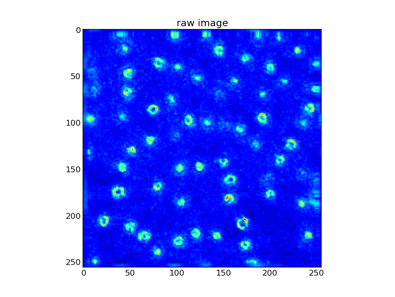
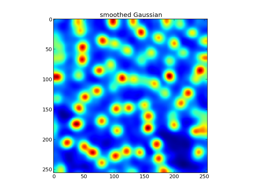
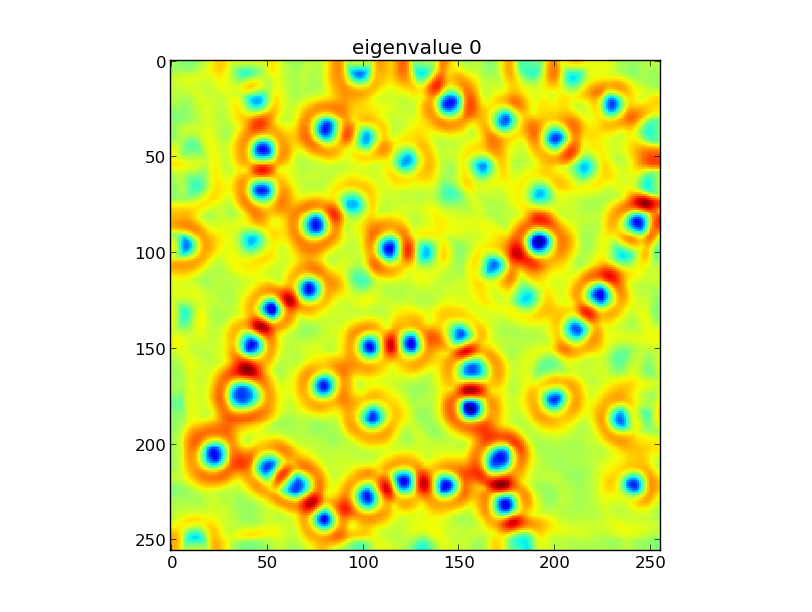
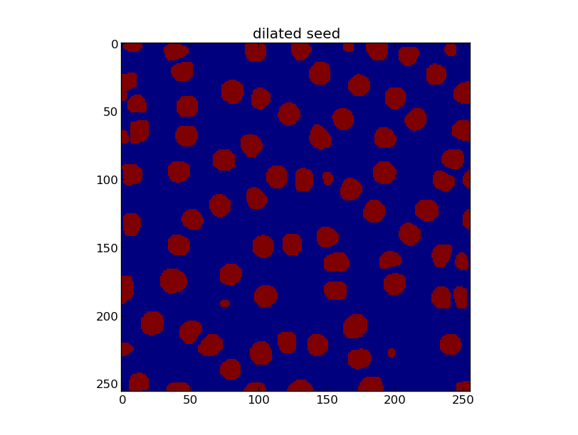
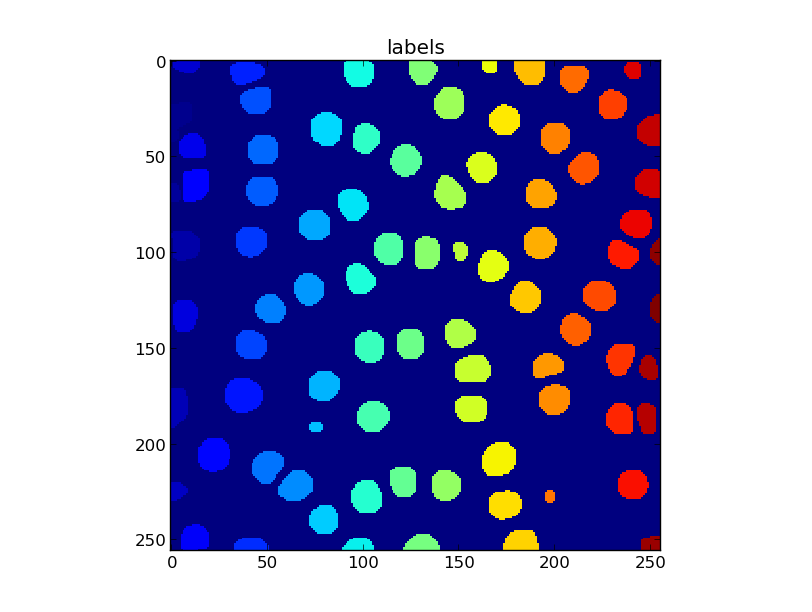
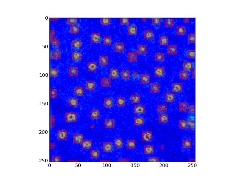
Therefore, simple thresholding of the eigenvalues can extract the foreground (cell). For a visualization of the individual steps of the method, see Figure 1. We repeat this procedure at different scales because a large Gaussian kernel strongly suppresses noise but yields merge errors (i.e., under-segmentation, because mass is aggregated within a larger neighborhood), while a small Gaussian kernel is sensitive to noise but better preserves the boundary. Results at different scales have characteristics that are complementary to each other and combing them produces less false positives and merge errors.

2.2 Parametric fits

Our method is optimized for the detection of cell nuclei, which are membrane enclosed organelles in eukaryotic cells that contain most of the cells genetic material. The shape of these objects resembles a deformed ellipsoid. We argue that we can incorporate this prior knowledge about the shape by fitting parametric geometric objects such as an $3D$ ellipsoid or stack of $2D$ ellipses.

(a) Parametric fit

(b) Layer 15 fit

(c) Layer 20 fit

Figure 2: Subfigure (a) gives an example of a parametric fit for a volume. Subfigure (b) and (c) show two slices through the volume in (a) for which a good parametric fit is obtained in the face of missing data points.

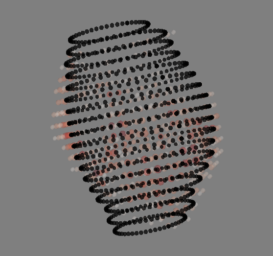
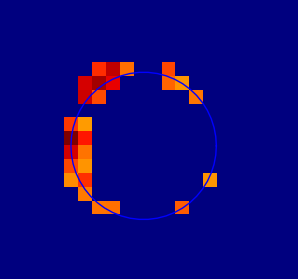
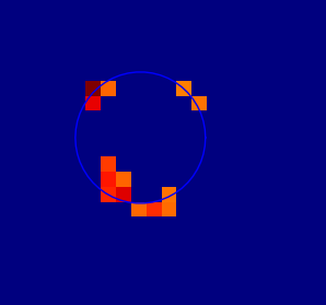
An example how parametric fitting is beneficial in providing robust fits in the face of missing data points is shown in Figure 2(c). While we limit ourselves to discussing ellipsoid structures for the rest of this paper, our framework generalizes to other geometric objects such as splines.

2.3 Fitting circles

We start with the simplest parametric object we could use for this task: a circle (one for each layer). This has obvious limitations, as many nuclei are not perfect circles, but rather correspond to ellipses in each layer. However, it may be easily derived and therefore constitutes a good starting point for the description of our method.

The distance of a point ${\boldsymbol{x}}\in\mathbb{R}^{2},i\in\{1,\dots,n\}$ to a circle with center ${\boldsymbol{c}}\in\mathbb{R}^{2}$ and radius $r\in\mathbb{R}$ is easily computed as

$$d({\boldsymbol{c}},r,{\boldsymbol{x}})=|\,\|{\boldsymbol{c}}-{\boldsymbol{x}}\|-r|$$

Finding a circle parametrized by ${\boldsymbol{c}}$ and $r$ that minimizes the sum of distances to points ${\boldsymbol{x}}_{i}$ corresponds to solving the following optimization problem:

$$\min_{{\boldsymbol{c}},r}\sum_{i=1}^{n}L(d({\boldsymbol{c}},r,{\boldsymbol{x}}_{i})),$$

where $L$ is a loss function, such as the squared loss or the hinge loss. The choice of loss function $L$ has important implications on the properties of the fit (e.g., robustness).

2.4 Fitting ellipses

A class of shapes that allows more flexibility for fitting nuclei in $2D$ are ellipses. An ellipse in $2D$ can be parametrized by a center point ${\boldsymbol{c}}=[c_{x},c_{y}]^{\top}$ and two radii ${\boldsymbol{r}}=[r_{x},r_{y}]^{\top}$ [Wei]. The points $[x,y]^{\top}$ on the ellipse centered at ${\boldsymbol{c}}$ are then given by the equation

$$\frac{(x-c_{x})^{2}}{r_{x}^{2}}+\frac{(y-c_{y})^{2}}{r_{y}^{2}}=1.$$ (1)

An alternate parametrization (general conic) is given by

$$ax^{2}+bxy+cy^{2}+dx+ey+f=0,$$ (2)

describing an ellipse if $b^{2}-4ac<0$ [Ros96]. Let

$${\boldsymbol{x}} =[x^{2},xy,y^{2},x,y,1],^{\top}$$ (3)

$$\Theta =[a,b,c,d,e,f]^{\top},$$

then points on the ellipse satisfy ${\boldsymbol{x}}^{\top}\Theta=0$. The algebraic distance $f$ of a point ${\boldsymbol{x}}$ to the ellipse parametrized by $\Theta$ is defined as:

$$f({\boldsymbol{x}},\Theta)={\boldsymbol{x}}^{\top}\Theta.$$ (4)

The algebraic distance is an approximation of the Euclidean distance that has the advantage that it is much easier to compute.

Avoiding degenerate solutions

Additional constraints are necessary to avoid degenerate solutions. In order to avoid the trivial solution $\Theta=0$ and recognizing that any multiple of a solution $\Theta$ represents the same conic, the parameter vector $\Theta$ is constrained in one way or the other [FPF99]. Different algorithms for fitting ellipses often only differ in the way they constrain parameters. Many authors suggest $\|a\|^{2}=1$, others $a+c=1$ or $f=1$ [FPF99].

Minimizing algebraic distance

For a general loss-function, we arrive at the following formulation:

$$\min_{\Theta} \sum_{i=1}^{N}L(\Theta^{\top}{\boldsymbol{x}}_{i})$$ (5)

s.t. solution non-degenerate

Depending on which combination of non-degeneracy constraints and loss function are used, different solvers are needed.

2.5 Robust Loss Function

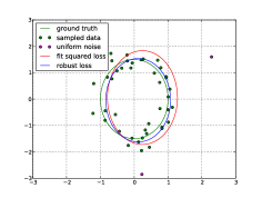
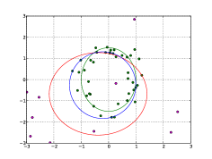
It is well established that the squared loss is particularly prone to outliers, as distance is penalized quadratically. An example of this sensitivity to outliers is shown in Figure 3, where a few outliers are sufficient to considerably distort the fit.

(a) Squared loss

(b) $\varepsilon$-insensitive loss

Figure 3: A severe effect of a few outliers for the squared loss is shown in (a). For the same data set, the $\varepsilon$-insensitive loss achieves a more robust solution as shown in (b).

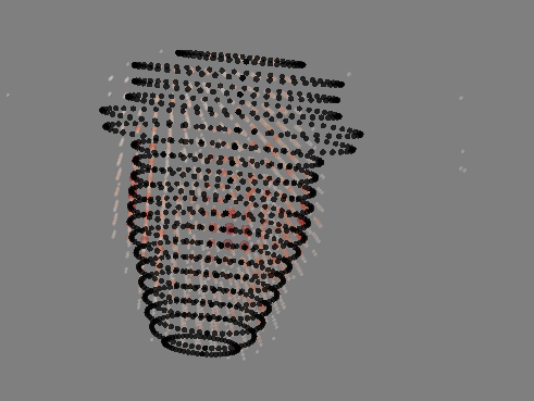
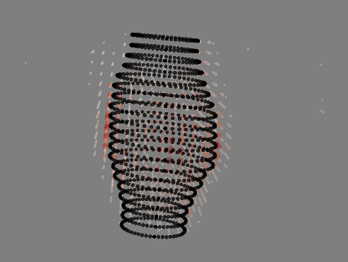
We therefore propose to use the $\varepsilon$-insensitive loss function for the problem at hand. The $\varepsilon$-insensitive loss has its background in the context of Support Vector Regression [Vap95, SS02, SS04]. It is also known as dead-zone penalty in other contexts [Boy04] and is often used when a more robust error function is needed.

$$L_{\varepsilon}(r)=\bigg{\{}\begin{array}[]{cl}|r|-\varepsilon,&\mbox{if }|r|>\varepsilon\\ 0&\mbox{else.}\end{array}$$ (8)

It has two important properties that make it appealing for the problem at hand. The first is that it does not penalize points that are within a rim of the stacked ellipsoid. This captures the intuition that the nuclear membrane has a certain thickness and we therefore do not want to penalize points that are within the membrane. Second, the loss is affine (linear minus some offset that depends on $\varepsilon$). This means that outliers are not penalized as severely as with the squared loss, yielding a more robust error function. In the following, we show that although non-differentiable, the $\varepsilon$-insensitive loss may be expressed in the form of a constrained optimization problem. As a first step, we note that $L_{\varepsilon}$ may be written as

$$L_{\varepsilon}(r)=\max(|r|-\varepsilon,0).$$ (9)

Plugging the above loss into Equation (5) and neglecting the non-degeneracy constraints for now, yields the optimization problem:

$$\min_{\Theta} \sum_{i=1}^{N}\max(|{\boldsymbol{x}}^{\top}\Theta|-\varepsilon,0).$$ (10)

We now make use of the fact that $\max(a,b)$ can be expressed to the smallest upper bound of $a$ and $b$ [Boy04], i.e.,

$$\max(a,b)=\min_{c}$$

s.t. $$a\leq c,$$ (11)

$$b\leq c.$$

Furthermore, we exploit that the absolute value may be expressed as the maximum of two linear functions $|r|=\max(r,-r)$. We use the latter to move $|{\boldsymbol{x}}^{\top}\Theta|$ from the objective to the constraints using newly introduced slack variables $s_{i}$. This gives rise to:

$$\min_{\Theta,s_{i}} \sum_{i=1}^{N}\max(s_{i}-\varepsilon,0)$$

s.t. $${\boldsymbol{x}}_{i}^{\top}\Theta\leq s_{i},$$ (12)

$$- {\boldsymbol{x}}_{i}^{\top}\Theta\leq s_{i}$$

Using the same scheme, the other $\max$ is moved to the constraints using Equation (11), introducing variables $t_{i}$. We arrive at:

$$\min_{\Theta,s_{i},t_{i}}\sum_{i=1}^{N} t_{i}$$

$$\textnormal{s.t. }{\boldsymbol{x}}_{i}^{\top}\Theta \leq s_{i},$$ (13)

$$-{\boldsymbol{x}}_{i}^{\top}\Theta \leq s_{i},$$

$$s_{i}-\varepsilon \leq t_{i},$$

$$0 \leq t_{i}.$$

2.6 Graph-regularization

To share information of the ellipse fitting across the z-layers , we propose to jointly fit ellipses in all layers and penalize differences between parameter vectors of neighboring layers by means of regularization term $R$:.

$$R(\Theta_{1},\dots,\Theta_{N})=\sum_{i=1}^{N-1}\|\Theta_{i}-\Theta_{i+1}\|_{p},$$ (14)

where $\|a\|_{p}$ is the $p$-norm. The effect of this smoothing is shown in Figure 4.

(a) No regularization

(b) Graph regularization

Figure 4: Example of cell fitting in each z-layer independently (a) and with graph regularization (b). In the top and bottom layers of the nucleus, the non-regularized $2D$ fits differ greatly between layers as only a few data points are available for each layer. By coupling layers via Multitask Regularization, we achieve a smooth fit.

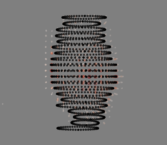
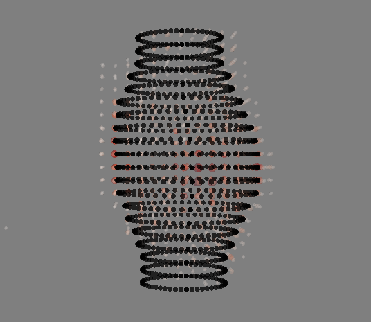
This smoothness regularizer is a special case of a general graph-regularizer, which is often used in the context of Multitask Learning [EMP05, WKGR12], as edges only exist between neighboring layers. Note that in the above formulation, we have not settled on a particular norm, however in the following we will instantiate to the $L_{1}$-norm.

2.7 Linear Program (LP) Formulation

We now start putting all pieces together to obtain the final optimization problem. Starting from Equation (13), we add the graph-regularizer from Equation (14) to the mix.

Note that to avoid the trivial solution, we add additional constraints as discussed in Section 2.4. Here, we use $\Theta_{i,1}+\Theta_{i,3}=1$ (i.e., $a+c=1$).

$$\min_{\Theta_{i},s_{i},t_{i}}\sum_{t=1}^{M}\sum_{i=1}^{N_{t}} t_{t,i}+\sum_{t=1}^{M-1}|\Theta_{i}-\Theta_{i+1}|_{1}$$

$$\textnormal{s.t. }{\boldsymbol{x}}_{i}^{\top}\Theta \leq s_{i},$$

$$-{\boldsymbol{x}}_{i}^{\top}\Theta \leq s_{i},$$

$$s_{i}-\varepsilon \leq t_{i},$$

$$0 \leq t_{i},$$

$$\Theta_{i,1}+\Theta_{i,3} =1.$$

Again, using the fact that $|a|=max(a,-a)$, we push the graph-regularizer to the constraints:

$$\min_{\Theta_{i},s_{i},t_{i}}\sum_{i=1}^{M}\sum_{j=1}^{N_{i}} t_{i,j}+\sum_{i=1}^{M-1}\sum_{j=1}^{D}u_{ij}$$

$$\textnormal{s.t. }\Theta_{i,j}-\Theta_{i,j} \leq u_{i,j}\forall i\in[1,M-1],j\in[1,D],$$

$$-\Theta_{i,j}+\Theta_{i,j} \leq u_{i,j}\forall i\in[1,M-1],j\in[1,D],$$

$${\boldsymbol{x}}_{i}^{\top}\Theta \leq s_{i},$$

$$-{\boldsymbol{x}}_{i}^{\top}\Theta \leq s_{i},$$

$$s_{i}-\varepsilon \leq t_{i},$$

$$0 \leq t_{i},$$

$$\Theta_{i,1}+\Theta_{i,3} =1.$$

The above problem consists of a linear objective and linear constraints and can therefore be solved with a linear program solver. We used the freely available GNU Linear Programing Toolkit to solve the above optimization problem (http://www.gnu.org/software/glpk/glpk.html).

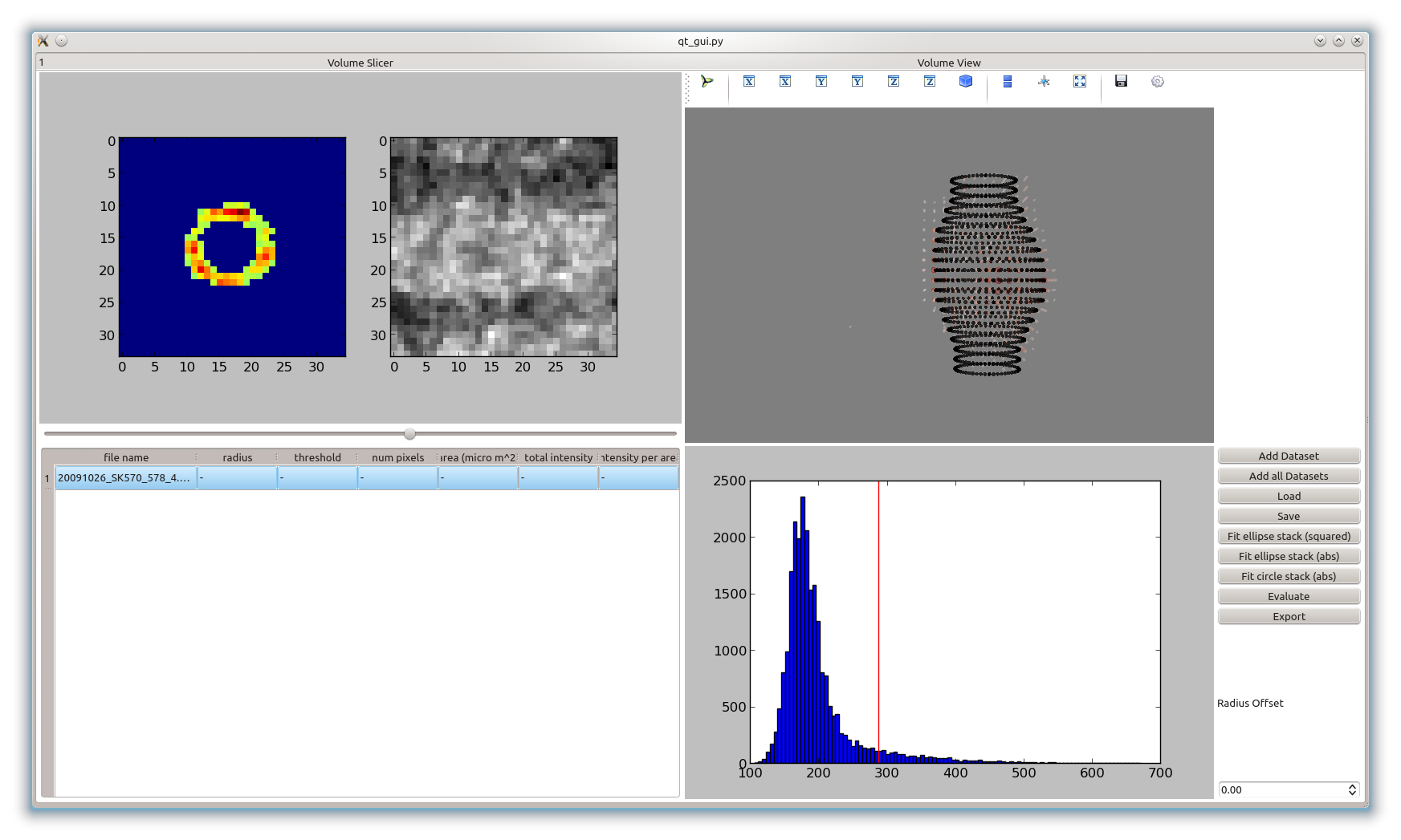
For ease of use, we provide a graphical user interface (GUI) as shown in Figure 5.

Figure 5: Graphical User Interface for rapidly performing experiments.

3 Experiments

Robustness Analysis

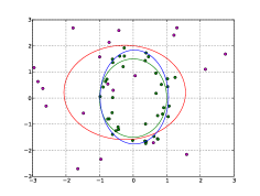
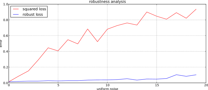
To compare robust loss and squared loss in the context of parametric fits, we set up an experiment using synthetic data. For this, we first sampled $n$ points ${\boldsymbol{x}}_{1},...,{\boldsymbol{x}}_{n}$ from an ellipse parametrized by $\Theta$. Next, uniformly distributed points were sampled in the interval $[-3,3]$ to simulate random noise and contaminations. Based on all sampled points, two fits were obtained, one using the squared loss and one using the robust loss. Examples of these fits are shown in 6(a), 6(b) and 6(c). A systematic comparison of the two losses is shown in Figure 7, where the error with respect to the ground truth (i.e., $\|\Theta_{fit}-\Theta\|$) is shown as a function of the number of uniformly sampled points. We observe that the error increases much later when using the robust loss function as opposed to using the squared loss.

(a) low noise

(b) medium noise

(c) high noise

Figure 6: Fits for different noise regimes. The dots that are sampled from the noise distribution are shown in (purple) and the ones sampled from the underlying ellipse (green) are shown in (black). The true squared loss fit is shown in (red) and the one using the robust loss is shown in (blue).

Figure 7: Comparison of the fitting error of the squared and robust loss for different mixtures of the distributions of the ellipsoid and the noise.

Evaluation in Practice

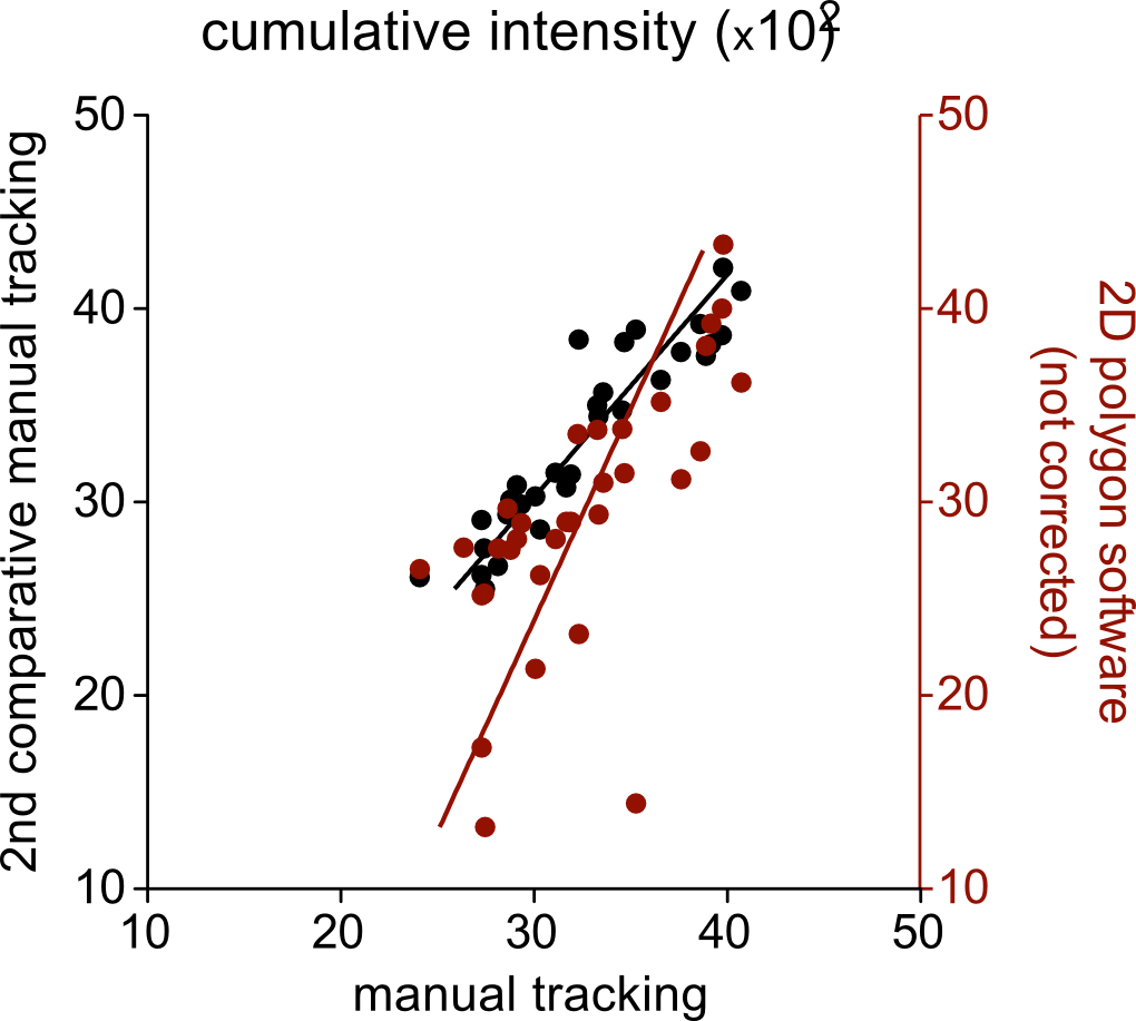
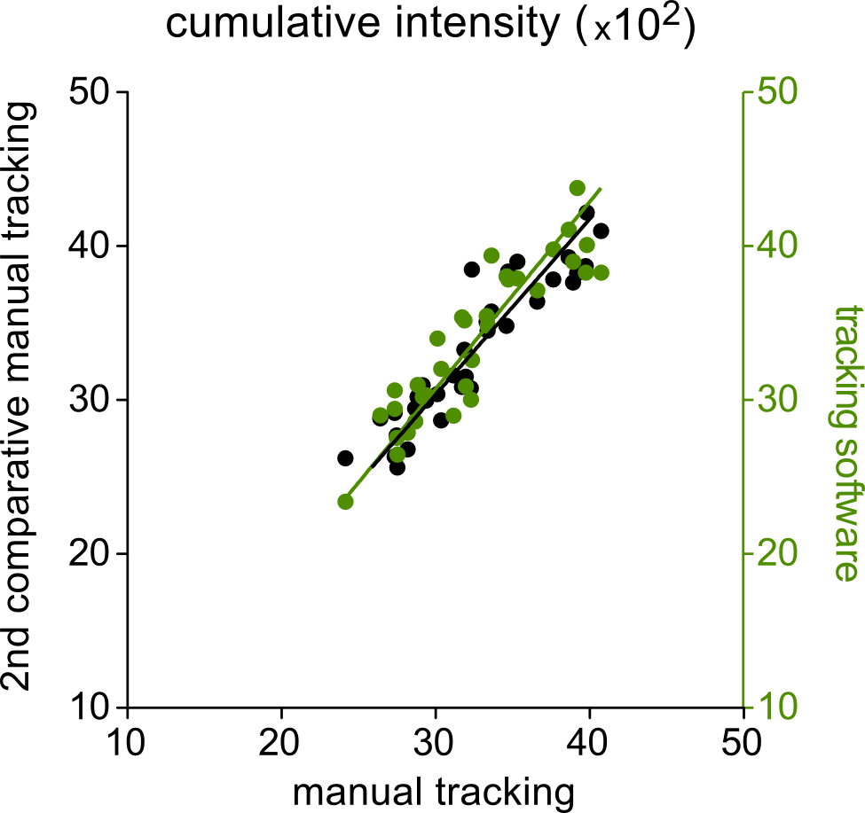
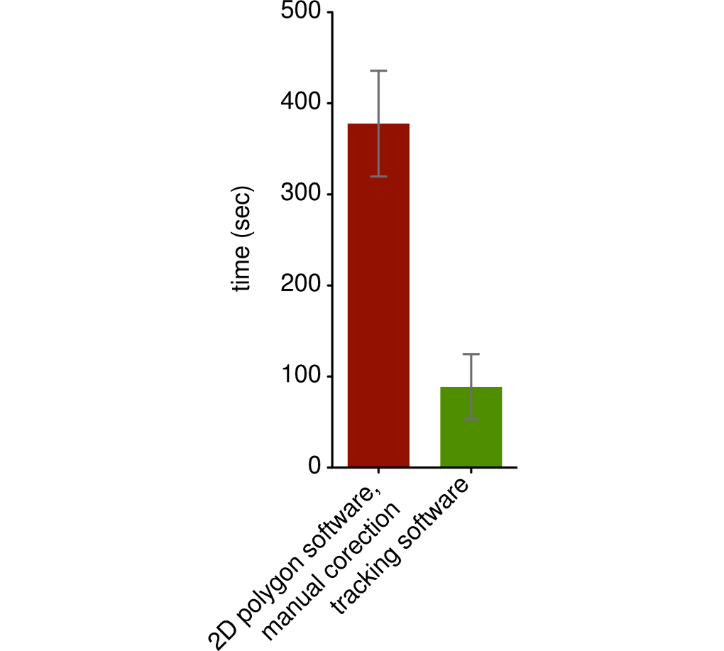
In order to evaluate the quality of our fits on real data, we compared them to manually curated segmentations obtained using the software of the microscope manufacturer. The results are shown in Figure 8(b). We observe that our approach has an almost perfect correlation to the manually curated ground truth, while the existing microscope software shows a considerable deviation (see Figure 8(a)). As we are ultimately interested in allowing for high-throughput experiments, we quantified the time taken to perform an experiment using our approach and the microscope software and report a large speed-up. Note that the experiment was conducted by fitting each cell individually. Taking into account the proposed preprocessing pipeline and setting up batch processing will almost entirely automate the procedure.

(a) Microscope software

(b) Our approach

(c) Time gain

Figure 8: Results on real data comparing the $2D$ polygon fit by the microscope manufacturer (a) to our approach (b). Taking into account manual post processing, the total time taken for an experiment is shown in (c).

4 Conclusion

We have presented a tool for parametric fitting of cell-like objects in fluorescence microscopy images. We have shown that using modern machine learning and computer-vision techniques, we can greatly speed-up the experimental process and outperform existing software. Combined with an easy-to-use user interface, our tool enables biologists to perform truly high-throughput quantitative experiments in fluorescence microscopy [HGK⁺13].

Acknowledgements

We gratefully acknowledge core funding from the Sloan-Kettering Institute (to G.R.), from the Ernst Schering foundation (to S.H.) and from the Max Planck Society (to G.R. and S.H.). Part of this work was done while C.W. P.D. and G.R. were at the Friedrich Miescher Laboratory of the Max Planck Society and while C.W. was at the Machine Learning Group at TU-Berlin.

References

- [Boy04] L. Boyd, S.P. and Vandenberghe. Convex optimization. Cambridge University Press, 2004.
- [EMP05] T. Evgeniou, C.A. Micchelli, and M. Pontil. Learning multiple tasks with kernel methods. Journal of Machine Learning Research, 6(1):615–637, 2005.
- [FPF99] A. Fitzgibbon, M. Pilu, and R.B. Fisher. Direct least square fitting of ellipses. Pattern Analysis and Machine Intelligence, IEEE Transactions on, 21(5):476–480, 1999.
- [GW08] R. C. Gonzalez and R. E. Woods. Digital Image Processing. Prentice Hall, Upper Saddle River, N.J., 2008.
- [HGK+13] S. Heinrich, E.M. Geissen, J. Kamenz, S. Trautmann, C. Widmer, P. Drewe, M. Knop, N. Radde, J. Hasenauer, and S. Hauf. Determinants of robustness in spindle assembly checkpoint signalling. Nature Cell Biology (in press), 2013.
- [LKWH12] X. Lou, U. Koethe, J. Wittbrodt, and F. A. Hamprecht. Learning to Segment Dense Cell Nuclei with Shape Prior. In CVPR, 2012.
- [Ros96] P.L. Rosin. Assessing error of fit functions for ellipses. Graphical models and image processing, 58(5):494–502, 1996.
- [SS02] B Schölkopf and A J Smola. Learning with Kernels, volume 64 of Adaptive Computation and Machine Learning. MIT Press, 2002.
- [SS04] A.J. Smola and B. Schölkopf. A tutorial on support vector regression. Statistics and Computing, 14(3):199–222, 2004.
- [Vap95] V N Vapnik. The Nature of Statistical Learning Theory, volume 8 of Statistics for Engineering and Information Science. Springer, 1995.
- [Wei] Eric W. Weisstein. Ellipse – from Wolfram MathWorld.
- [WKGR12] C. Widmer, M. Kloft, N. Görnitz, and G. Rätsch. Efficient Training of Graph-Regularized Multitask SVMs. In ECML2012, 2012.