Intrinsic decoherence in the interaction of two fields with a two-level atom

Abstract

We study the interaction of a two-level atom and two fields, one of them classical. We obtain an effective Hamiltonian for this system by using a method recently introduced that produces a small rotation to the Hamiltonian that allows to neglect some terms in the rotated Hamiltonian. Then we solve a variation of the Schrödinger equation that models decoherence as the system evolves through intrinsic mechanisms beyond conventional quantum mechanics rather than dissipative interaction with an environment.

I Introduction

The study the interaction between a two-level atoms and quantized single-mode fields prepared initially in specific states such as binomial states Orany , displaced number states Moya , etc. has attracted the attention over the years because of the possibilities of engineering more interesting states of the electromagnetic field Moya2 ; Moya3 . Usually the atom-field entanglement in such states is very sensitive to dissipation and decoherence Ge ; Yu ; Xu , and the states are rapidly degraded to statistical mixtures.

It is complicated to find analytical solutions for problems that include dissipation if Hamiltonians are not simplified. Such simplification is possible under certain circumstances if the parameters involved allow to obtain effective Hamiltonians, either by the use of the adiabatic elimination Larson or by the use of other approaches such as the small rotation method Klimov . When dissipation is included before effective Hamiltonians are developed, the problem usually may only be solved numerically. Here we apply the later method to obtain an effective Hamiltonian for the interaction of a two-level atom and two fields, one quantized and the other classical and solve a variation of the Schrödinger equation that models decoherence as the system evolves through intrinsic mechanisms beyond conventional quantum mechanics rather than dissipative interaction with an environment Milburn .

The atom interacting with two fields has been studied when both fields are quantized Dutra and for the case in which one of them is considered classical Alsing finding in this last case the appearance of super-revivals Dutra2 .

II Atom-Two Fields Effective Hamiltonian

The Hamiltonian for a two-level atom interacting with a quantized field and a classical field is given by Alsing (we set $\hbar=1$)

$$H=\omega a^{\dagger}a+\omega_{0}\frac{\sigma_{z}}{2}+\lambda(a^{\dagger}\sigma_{-}+\sigma_{+}a)+\epsilon e^{-i\omega t}\sigma_{+}+\epsilon^{*}e^{i\omega t}\sigma_{-}$$ (1)

where $a$ and $a^{\dagger}a$ are the annihilation and creation operators, respectively, $\omega$ is the frequency of both quantized and classical fields, the $\sigma$’s are the spin Pauli matrices, $\lambda$ is the interaction constant between the atom and the quantized field, $\omega_{0}$ is the atomic transition frequency and $\epsilon$ is the amplitude of the classical field.

We may get rid off the time dependence by transforming the Hamiltonian with $T=\exp[-i(\omega a^{\dagger}a+\omega\frac{\sigma_{z}}{2})t]$ and obtain the interaction Hamiltonian

$$H_{\rm I}=\Delta\frac{\sigma_{z}}{2}+\lambda(a^{\dagger}\sigma_{-}+\sigma_{+}a)+\epsilon\sigma_{+}+\epsilon^{*}\sigma_{-}$$ (2)

with $\Delta=\omega_{0}-\omega$. We consider the strong detuning case $|\Delta|\gg\lambda,\epsilon$ and produce a small rotation to the interaction Hamiltonian, namely, we transform it with $R=\exp[\eta(a^{\dagger}\sigma_{-}-\sigma_{+}a)]$ with the parameter $\eta\ll 1$, such that we may approximate $RAR^{\dagger}\approx A+\eta[(a^{\dagger}\sigma_{-}-\sigma_{+}a),A]$, with $A$ an arbitrary operator. By taking $A=H_{I}$ and setting $\eta=-\lambda/\Delta$, we obtain the effective Hamiltonian

$$H_{\rm eff}=\sigma_{z}\left[\frac{2\lambda^{2}}{\Delta}(2N+1)+\frac{2\lambda}{\Delta}(\epsilon a^{\dagger}+\epsilon^{*}a)+\frac{\Delta}{2}\right]+\epsilon\sigma_{+}+\epsilon^{*}\sigma_{-},$$ (3)

with $N=a^{\dagger}a$, the number operator. By displacing the Hamiltonian above with the Glauber displacement operator Glauber , we obtain

$$H_{\rm eff}=D(\beta)\left\{\sigma_{z}\left[\chi N+{\tilde{\Delta}}\right]+\epsilon\sigma_{+}+\epsilon^{*}\sigma_{-}\right\}D^{\dagger}(\beta),$$ (4)

with $\chi=-2\lambda^{2}/\Delta$, $\beta=\eta/\chi$ and $\tilde{\Delta}=\Delta-|\epsilon|^{2}/\chi$ and its evolution operator may be easily obtained

$$U_{\rm eff}(t)=D^{\dagger}(\beta)e^{-it\left(\sigma_{z}\left[\chi N+{\tilde{\Delta}}\right]+\epsilon\sigma_{+}+\epsilon^{*}\sigma_{-}\right)}D(\beta),$$ (5)

with

$$e^{-it\left(\sigma_{z}\left[\frac{2\lambda^{2}}{\Delta}2N+\frac{\tilde{\Delta}}{2}\right]+\epsilon\sigma_{+}+\epsilon^{*}\sigma_{-}\right)}=\left[\begin{array}[]{cc}U_{\rm 11}&U_{\rm 12}\\ U_{\rm 21}&U_{\rm 22}\end{array}\right]$$ (6)

where we have used the $2\times 2$ matrix representation of the Pauli spin operators. The matrix elements are given by

$$U_{\rm 11}(t)=\cos[\Omega_{N}t]-i\frac{\chi N+\tilde{\Delta}}{\Omega_{\rm N}}\sin[\Omega_{N}t],$$

$$U_{\rm 12}(t)=-i\frac{\epsilon}{\Omega_{\rm N}}\sin[\Omega_{\rm N}t]$$

$$U_{\rm 21}(t)=-i\frac{\epsilon^{*}}{\Omega_{\rm N}}\sin[\Omega_{\rm N}t]$$

$$U_{\rm 22}(t)=\cos[\Omega_{\rm N}t]+i\frac{\chi N+\tilde{\Delta}}{\Omega_{\rm N}}\sin[\Omega_{\rm N}t],$$ (7)

with $\Omega_{\rm N}=\sqrt{(\chi N+\tilde{\Delta})^{2}+|\epsilon|^{2}}$.

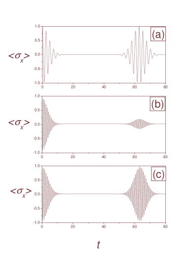
Figure 1: We plot $\langle\sigma_{\rm x}\rangle$ for the following parameters: (a) $\alpha=2.5$, $E=0$, $\lambda=1$, $\Delta=2$ and $\gamma=10^{6}$, (b) $\alpha=2.5$, $E=0.5$, $\lambda=1$, $\Delta=2$ and $\gamma=10^{3}$ and (c) $\alpha=2.5$, $E=0.5$, $\lambda=1$, $\Delta=2$ and $\gamma=10^{6}$.

III Intrinsic Decoherence

There have been proposals in which the Schrödinger equation is modified such that quantum coherences are destroyed as the system evolves. Milburn Milburn has proposed a model of intrinsic decoherence that is a modification of quantum mechanics based on the assumption that on sufficiently short time steps the system does not evolve continuously under unitary evolution but rather in an stochastic sequence of identical unitary transformations. The differential equation for the density matrix in Milburn’s model reads

$$\frac{d\rho}{dt}=\gamma(e^{-iH/\hbar\gamma}\rho e^{iH/\hbar\gamma}-\rho)$$ (8)

with $\rho$ the density matrix and $\gamma$ is the rate at which coherences are lost and is related with the minimum time step in the universe Milburn . By expanding (8) to first order in $\gamma^{-1}$ Milburn obtained the following equation

$$\frac{d\rho}{dt}=\frac{i}{\hbar}[H,\rho]-\frac{1}{2\hbar^{2}\gamma}[H,[H,\rho]].$$ (9)

Note that taking $\gamma\rightarrow\infty$ Schrödinger equation is recovered. We now solve equation (8) instead of the approximated (9) for the Hamiltonian (4)

$$\rho(t)=e^{-\gamma t}\sum_{m=0}^{\infty}\frac{(\gamma t)^{m}}{m!}e^{-imH_{\rm eff}/\gamma}\rho(0)e^{imH_{\rm eff}/\gamma}.$$ (10)

By doing $t\rightarrow m/\gamma$ in eq. (5), we can easily evaluate the above solution for any initial condition for the atom and the field. Let us consider the atom initially in a superposition of ground and excited states

$$|\psi_{A}(0)\rangle=\frac{1}{\sqrt{2}}(|g\rangle+|e\rangle)$$ (11)

and the field initially in a coherent state Glauber

$$|\alpha\rangle=D(\alpha)|0\rangle,$$ (12)

we may then express the initial density matrix in the atomic $2\times 2$ basis as

$$\rho(0)=\frac{|\alpha\rangle\langle\alpha|}{2}\left[\begin{array}[]{cc}1&1\\ 1&1\end{array}\right].$$ (13)

We have now all the ingredients to obtain expectation values of atomic and field observables. For instance, we can calculate the atomic polarization $\langle\sigma_{x}\rangle$, a common expectation value used in the reconstruction of the Wigner function

$$\langle\sigma_{\rm x}\rangle= e^{-|\alpha-\beta|^{2}}\sum_{n=0}^{\infty}\frac{|\alpha-\beta|^{2n}}{n!\Omega_{\rm n}^{2}}$$ (14)

$$\left(\epsilon^{2}+e^{-\gamma t(1-\cos(2\Omega_{\rm n}/\gamma))}(\chi n+\tilde{\Delta})^{2}\cos(\gamma t\sin(2\Omega_{\rm n}/\gamma))\right).$$

We plot the atomic polarization in Fig. 1, where we can see revivals and collapses of this observable (a) for the parameter $\gamma=10^{6}\lambda$, and no classical field ($\epsilon=0$); degradation of the revivals may be seen in (b) where the parameter $\gamma=10^{3}\lambda$ has been reduced, and the classical field is present ($\epsilon=0.5\lambda$), and the effects of the intrinsic decoherence are clear and in (c) we again set $\gamma=10^{6}\lambda$ for the classical field as in (b) and the revivals are recovered.

IV Conclusions

We have studied the interaction of a two-level atom and two fields, one of them classical in the dispersive regime by using a model of intrinsic decoherence that has been shown to degrade the revivals of the atomic polarization. It was given a solution for the exact equation 8 rather than the approximated one 9. The dispersive Hamiltonian was obtained by using the method of small rotations Klimov .

We would like to thank CONACYT for support.

References

- (1) F.A.A. El-Orany, Ann. Phy. (Berlin) 17, 424 (2008).
- (2) F.A.M. de Oliveira, M.S. Kim, P.L. Knight, and V. Buzek, Phys. Rev. A 41 2645 (1990).
- (3) H. Moya-Cessa and A. Vidiella-Barranco, Journal of Modern Optics 39, 2481 (1992).
- (4) H. Moya-Cessa and A. Vidiella-Barranco, Journal of Modern Optics 42, 1547 (1995).
- (5) M. Ge, L.-F. Zhu, and L. Qiu, Ann. Phys. (Berlin) 17, 336 (2008).
- (6) P.-F. Yu, J.-G. Cai, J.-M. Liu, and G.-T. Shen, Physica A 387, 4723 (2008).
- (7) X.-B. Xu, J.-M. Liu, and P.-F. Yu, Chinese Physics B 17, 1674 (2008).
- (8) J. Larson, S. Fernández-Vidal, G. Morigi, and M. Lewenstein, New J. Phys. 10 , 045002 (2008).
- (9) A.B. Klimov and L.L. Sánchez-Soto, Phys. Rev. A 61, 063802 (2000).
- (10) G.J. Milburn, Phys. Rev. A 48, 5401 (1991).
- (11) S.M. Dutra, P.L. Knight, and H. Moya-Cessa, Phys. Rev. A 48, 3168 (1993).
- (12) P. Alsing, D.-S. Guo, and H.J. Carmichael, Phys. Rev. A 45, 5135 (1992).
- (13) S.M. Dutra, P.L. Knight, and H. Moya-Cessa, Phys. Rev. A 49, 1993 (1994).
- (14) R.J. Glauber, Phys. Rev. A 131, 2766 (1963).