Error estimates for approximations of nonhomogeneous nonlinear uniformly elliptic equations

Abstract.

We obtain an error estimate between viscosity solutions and $\delta$-viscosity solutions of nonhomogeneous fully nonlinear uniformly elliptic equations. The main assumption, besides uniform ellipticity, is that the nonlinearity is Lipschitz-continuous in space with linear growth in the Hessian. We also establish a rate of convergence for monotone and consistent finite difference approximation schemes for such equations.

1. Introduction

We prove an estimate between viscosity solutions and $\delta$-viscosity solutions of the boundary value problem

(1.1) $$\left\{\begin{array}[]{l l}F(D^{2}u,x)=f(x)&\quad\text{ in }U\subset\mathbb{R}^{n},\\ u=g&\quad\text{ on }\partial U,\end{array}\right.$$

where $F$ is uniformly elliptic (see (F1) below) and Lipschitz-continuous in space with linear growth in the Hessian (see (F2) below). As a consequence, we find a rate of convergence for monotone and consistent finite difference approximations to (1.1). Both results generalize the work of Caffarelli and Souganidis in [6, 7], who consider either homogeneous equations or equations with separated dependence on the space variable and on the Hessian.

The nonlinearity $F$ is a continuous function on $\mathcal{S}_{n}\times U$, where $\mathcal{S}_{n}$ is the set of $n\times n$ real symmetric matrices endowed with the usual order and norm (for $X\in\mathcal{S}_{n}$, $||X||=\sup_{|v|=1}|Xv|$). We make the following assumptions:

1. $F$ is uniformly elliptic, which means there exist constants $0<\lambda\leq\Lambda$ such that for all $x\in U$, any $X\in\mathcal{S}_{n}$, and for all $Y\geq 0$,

   $$\lambda||Y||\leq F(X+Y,x)-F(X,x)\leq\Lambda||Y||;$$

   and,

2. there exists a positive constant $\kappa$ such that for all $x,y\in U$ and all $X\in\mathcal{S}_{n}$,

   $$|F(X,x)-F(X,y)|\leq\kappa|x-y|(||X||+1).$$

An example of an equation satisfying our assumptions is the Isaacs equation

$$F(D^{2}u,x)=\sup_{\alpha}\inf_{\beta}L^{\alpha,\beta}u(x),$$

where, for each $\alpha$ and $\beta$ in some index sets, the operator $L^{\alpha,\beta}$ is given by

$$L^{\alpha,\beta}u(x)=\sum_{i,j=1}^{n}a_{ij}^{\alpha,\beta}(x)\partial^{2}_{i,j}u(x)+f^{\alpha,\beta}(x),$$

and is uniformly elliptic with uniformly Lipschitz coefficients, which means there exists a $\kappa$ such that for all $x,y\in U$ and for all $\alpha$, $\beta$, $i$ and $j$,

$$|a_{ij}^{\alpha,\beta}(x)-a_{ij}^{\alpha,\beta}(y)|\leq\kappa|x-y|$$

and

$$|f^{\alpha,\beta}(x)-f^{\alpha,\beta}(y)|\leq\kappa|x-y|.$$

The Isaacs equation arises in the study of stochastic differential games. We do not give further details about the Isaacs equation and refer the reader to Section 1 of Crandall, Ishii and Lions’ [8] for a list of references.

We also assume:

1. $U$ is a bounded subset of $\mathbb{R}^{n}$ with regular boundary,

1. $f\in C^{0,1}(U)$, and

2. $g\in C^{1,\gamma}(\partial U)$ for some $\gamma\in(0,1]$.

The main result is a comparison between solutions and $\delta$-viscosity solutions (briefly, $\delta$-solutions) of (1.1). The definition of $\delta$-solutions is given in Section 2.2. Next we present a statement of our main result that has been simplified for the introduction; the full statement is in Section 7.

Theorem 1.1.

Assume (U1), (F1), (F2), (G1), (G2). Let $u$ be a viscosity solution of (1.1) and assume that $\left\{v_{\delta}\right\}_{\delta\geq 0}$ is a family of Hölder continuous $\delta$-solutions of (1.1) that satisfy, for all $\delta>0$,

$$v_{\delta}=u\text{ on }\partial U.$$

There exist positive constants $\bar{\delta}$, $\bar{\alpha}$ and $\bar{c}$ such that, for any $\delta\leq\bar{\delta}$,

$$\sup_{U}|u-v_{\delta}|\leq\bar{c}\delta^{\bar{\alpha}}.$$

The notion of $\delta$-solutions was introduced in [7] for fully nonlinear uniformly elliptic equations of the form $F(D^{2}u)=0$. An error estimate between solutions and $\delta$-solutions of such equations was established in [7]. A key step in the proof of the error estimate was a regularity result ([6, Theorem A]), which says that, outside of sets of small measure, solutions of $F(D^{2}u)=f(x)$ have second-order expansions with controlled error. The proof of this regularity theorem relies on the equation being homogeneous – differentiating $F(D^{2}u)=f(x)$ implies that the derivatives $u_{x_{i}}$ solve the linear uniformly elliptic equation $\operatorname{tr}(DF\cdot D^{2}u_{x_{i}})=f_{x_{i}}$; therefore, a known estimate that gives first-order expansions on large sets (see Chapter 7 of Caffarelli and Cabre [5]) applies to $u_{x_{i}}$, and from this the estimates on $u$ are deduced.

The main challenge in the $x$-dependent case is that this extra regularity result is not known. Because differentiating the $x$-dependent equation $F(D^{2}u,x)=f(x)$ does not imply anything useful about the derivatives of $u$, we cannot hope to replicate the proof of [6, Theorem A] for non-homogeneous equations.

Let us briefly describe the strategy of proof of Theorem 1.1. We perturb the nonlinearity $F$ and then “localize” the equation (see Propositions 4.2 and 3.1). This allows us obtain an approximation of $u$ that is regular enough to compare to the $\delta$-solution $v_{\delta}$. We hope that this method, in particular the use of the perturbations of $F$, may be of interest in other contexts. We include a detailed outline in Section 2.4.

Remark 1.2.

The assumption (F2) on the nonlinearity $F$ may be weakened. In fact, there exists a universal constant $\alpha$ such that if $\beta>1-\alpha$, our results hold for any $F$ that satisfies

$$|F(X,x)-F(X,y)|\leq\kappa(1+||X||)|x-y|^{\beta}.$$

This requirement on $\beta$ comes from the proof of Proposition 3.1, and $\alpha$ is the exponent from Proposition 2.5. For simplicity, we will only work with the case $\beta=1$ (in other words, we assume that $F$ satisfies (F2)).

Remark 1.3.

We often assume

(1.2) $$F(0,x)=0\text{ for all }x\in U.$$

This is not a restrictive assumption: the equation $F(D^{2}u,x)=f(x)$ is equivalent to $F(D^{2}u,x)-F(0,x)=f(x)-F(0,x)$, and the nonlinearity $\tilde{F}(M,x)=F(M,x)-F(0,x)$ satisfies (1.2).

We also study finite difference approximations to (1.1). We write the finite difference approximations as

(1.3) $$\left\{\begin{array}[]{l l}F_{h}[v_{h}](x)=0&\quad\text{ in }U_{h},\\ v_{h}=g&\quad\text{ on }\partial U_{h},\end{array}\right.$$

where $U_{h}=U\cap h\mathbb{Z}^{n}$ is the mesh of discretization and $F_{h}$ is the finite difference operator. We assume:

1. if $v_{h}^{1}$ and $v_{h}^{2}$ satisfy $F_{h}[v_{h}](x)=0$ in $U_{h}$ and $v_{h}^{1}\leq v_{h}^{2}$ on $\partial U_{h}$, then $v_{h}^{1}\leq v_{h}^{2}$ on $U_{h}$; and

2. there exists a positive constant $K$ such that for all $\phi\in C^{3}(U)$ ,

   $$|F_{h}[\phi](x)-(F(D^{2}\phi,x)-f(x))|\leq K(1+||D^{3}\phi||_{L^{\infty}(U)})h\text{ in }U.$$

Schemes that satisfy ($F_{h}$1) and ($F_{h}$2) are said to be, respectively, monotone and consistent with an error estimate for $F$.

We have simplified our notation here in order to state our main result; all the details about approximation schemes and the precise statement of Theorem 1.4 are given in Sections 8 and 9. We prove:

Theorem 1.4.

Assume (U1), (F1), (F2), (G1), and suppose $g\in C^{1,\gamma}(U)$. Assume that $F_{h}$ is a monotone scheme that is consistent with an error estimate for $F$. Assume that $u$ is the viscosity solution of (1.1) and that $v_{h}$ satisfies (1.3). There exist positive constants $\bar{c}$, $\bar{\alpha}$ and $\bar{h}$ such that for all $h\leq\bar{h}$,

$$\sup_{U_{h}}|u-v_{h}|\leq\bar{c}h^{\bar{\alpha}}.$$

The convergence of monotone and consistent approximations of fully nonlinear second order PDE was first established by Barles and Souganidis [3]. Kuo and Trudinger [15, 16] later studied the existence of monotone and consistent approximations for nonlinear equations and the regularity of the approximate solutions $u_{h}$. They showed that if $F$ is uniformly elliptic, then there exists a monotone finite difference scheme $F_{h}$ that is consistent with $F$, and that the approximate solutions $v_{h}$ are in $C^{0,\eta}$. However, obtaining an error estimate remained an open problem.

The first error estimates for approximation schemes were established by Krylov for equations that are either convex or concave, but possibly degenerate [12, 13]. Krylov used stochastic control methods that apply in the convex or concave case, but not in the general setting. Barles and Jakobsen in [1, 2] improved Krylov’s error estimates for convex or concave equations. In [14] Krylov improved the error estimate to be of order $h^{1/2}$, but still in the convex/concave case. In addition, Jakobsen [10, 11] and Bonnans, Maroso, and Zidani [4] established error estimates for special equations or for special dimensions. The first error estimate for general nonlinear equations that are neither convex nor concave was obtained by Caffarelli and Souganidis in [6]. Their result holds for equations $F$ that do not depend on $x$.

To our knowledge, Theorem 1.4 is the first error estimate for general nonlinear uniformly elliptic equations that are neither convex nor concave and are not homogeneous. In particular, this is the first error estimate for approximations of the Isaacs equation. To prove Theorem 1.4, we show that an appropriate regularization of the solution of (1.3) is a $\delta$-solution of (1.1), where $\delta$ depends on $h$ (see Proposition 8.4). This allows us to essentially deduce Theorem 1.4 from our estimate in Theorem 1.1.

Our paper is structured as follows. In Section 2 we establish notation, give the definition of $\delta$-solutions and state several known results about the regularity of viscosity solutions of (1.1). We provide a detailed outline of the proofs of our main results in Section 2.4. Section 3 is devoted to establishing an estimate between the solution $u$ of (1.1) and solutions of the equation with “frozen coefficients” on small balls. This is Proposition 3.1. In Section 4 we study perturbations of the equation (1.1) and prove an estimate between $u$ and solutions of the perturbed equations (Proposition 4.2). In Section 5 we establish an elementary lemma that plays an important role in the proofs of Theorems 1.1 and 1.4. Section 6 is devoted to the statement and proof of an important estimate between $\delta$-solutions of (1.1) and solutions of equations with frozen coefficients. This is Proposition 6.1. The full statement and the proof of our main result, Theorem 1.1, is in Section 7. Section 8 is devoted to introducing the necessary notation and stating known results about approximation schemes. In Proposition 8.4 we show that certain regularizations of the approximate solutions $v_{h}$ are $\delta$-solutions of (1.1). In Section 9 we give the precise statement and proof of Theorem 1.4. In Appendix A we state several known results related to the comparison principle for viscosity solutions. In Appendix B we summarize the properties of inf- and sup- convolutions that we use in our paper.

Contents

1. 1 Introduction
2. 2 Preliminaries and outline
   1. 2.1 Notation
   2. 2.2 Notions of solution
   3. 2.3 Known results
      1. 2.3.1 Regularization by inf- and sup- convolution
   4. 2.4 Outline of the proof of the main results
3. 3 The estimate between the solution of (1.1) and solutions of (1.1) with fixed coefficients.
4. 4 Perturbations of the nonlinearity
5. 5 An elementary lemma
6. 6 A key estimate between solutions and sufficiently regular $\delta$-solutions
   1. 6.1 Outline of the proof of Proposition 6.1
   2. 6.2 An auxiliary lemma
   3. 6.3 Proof of Proposition 6.1
   4. 6.4 Proof of auxiliary lemma
7. 7 Proof of Theorem 1.1
8. 8 Approximation schemes
   1. 8.1 Inf and sup convolutions of mesh functions
9. 9 Proof of Theorem 1.4
10. A
11. B
    1. B.1 Inf and sup convolutions of mesh functions

2. Preliminaries and outline

In this section we establish notation, give the definition of $\delta$-solutions, recall some known results, and provide an outline of our argument.

2.1. Notation

We denote open balls in $\mathbb{R}^{n}$ by

$$B_{r}(x_{0})=B(x_{0},r)=\{x\in\mathbb{R}^{n}:\ \ |x-x_{0}|<r\},$$

and we often write $B_{r}$ to mean $B_{r}(0)$. We denote the diameter of $U\subset\mathbb{R}^{n}$ by $\operatorname{diam}U$. A paraboloid $P(x)$ is a polynomial in $x_{1},...,x_{n}$ of degree 2. We say that a paraboloid $P$ is of opening $M$ if

$$P(x)=l(x)+M\frac{|x|^{2}}{2},$$

where $l$ is an affine function and $M$ is a constant.

Throughout the paper we say a constant is universal if it is positive and depends only on $n$, $\lambda$, and $\Lambda$.

2.2. Notions of solution

We consider solutions of (1.1) in the viscosity sense; see [8] for an introduction to the theory of viscosity solutions. Throughout, we say “solution” to mean “viscosity solution.”

Definition 2.1.

We say that $v$ is a $\delta$-subsolution (respectively, $\delta$-supersolution) of (1.1) if, for any $x$ such that $B_{\delta}(x)\subset U$, any paraboloid $P$ with $P(x)=v(x)$ and $P(y)\geq v(y)$ (respectively, $P(y)\leq v(y)$) for all $y$ in $B_{\delta}(x)$ satisfies

$$F(D^{2}P,x)\geq 0\text{ (respectively, $F(D^{2}P,x)\leq 0$)}.$$

We say that $v$ is a $\delta$-solution if $v$ is both a $\delta$-subsolution and a $\delta$-supersolution.

From the definition, it is clear that a viscosity solution of (1.1) is a $\delta$-solution of (1.1) for any $\delta>0$. The difference from the definition of viscosity solution is that for $u\in C(U)$ to be a $\delta$-supersolution (resp. $\delta$-subsolution), any test paraboloid must stay below (resp. above) $u$ on a set of fixed size.

2.3. Known results

We recall that the concave envelope of a function $u\in C(B_{r})$ is defined as

$$\Gamma_{u}(x)=\inf\{l(x):\ l\geq u\text{ in $B_{r}$ and $l$ is affine}\}.$$

In addition, we will use the following terminology:

Definition 2.2.

For $u\in C(U)$, we say $D^{2}u(x)\geq MI$ (resp. $D^{2}u\leq MI$) in the sense of distributions if there exists a paraboloid $P$ of opening $M$ such that $u(x)=P(x)$ and, for all $y\in B_{r}(x)$ for some $r$,

$$u(y)\geq P(y)\text{ (resp. }u(y)\leq P(y)).$$

The following fact is a key step in the proof of the well-known Alexander-Bakelman-Pucci (ABP) estimate, and it will play a central role in our arguments. It is Lemma 3.5 of the book of Caffarelli and Cabre [5], modified slightly for our setting.

Proposition 2.3.

Assume $u\in C(B_{r})$ is such that $u\leq 0$ on $\partial B_{r}$. Assume that there exists a constant $K$ such that $D^{2}u(x)\geq K$ in the sense of distributions for all $x\in B_{r}$. There exists a universal constant $C$ such that

$$\sup_{B_{r}}u\leq Cr\left(\int_{\{u=\Gamma_{u}\}}|\det D^{2}\Gamma_{u}|\right)^{\frac{1}{n}},$$

where $\Gamma_{u}$ is the concave envelope of $u^{+}$ in $B_{2r}$. Moreover, $\Gamma_{u}$ is twice differentiable almost everywhere.

Next we provide the statements of several known regularity results, for which we introduce the adimensional $C^{1,\alpha}$ norm, denoted by $||\cdot||_{C^{1,\alpha}(\bar{B}_{r})}^{*}$:

$$||u||_{C^{1,\alpha}(\bar{B}_{r})}^{*}=||u||_{L^{\infty}(B_{r})}+r||Du||_{L^{\infty}(B_{r})}+r^{1+\alpha}[Du]_{C^{0,\alpha}(B_{r})}.$$

We need the following rescaled version of the interior $C^{1,\alpha}$ estimate [5, Corollary 5.7].

Proposition 2.4 (Interior estimate).

Assume (F1). There exist universal constants $\alpha$ and $C$ such that if $u$ is a viscosity solution of $F(D^{2}u)=0$ in $B_{r}$, then $u\in C^{1,\alpha}(\bar{B}_{r/2})$ and

$$||u||_{C^{1,\alpha}(\bar{B}_{r/2})}^{*}\leq C(||u||_{L^{\infty}(B_{r})}+|F(0)|).$$

In addition to the interior $C^{1,\alpha}$ interior estimate, we need the following global $C^{1,\alpha}$ estimate (Winter [17, Theorem 3.1, Proposition 4.1]).

Proposition 2.5 (Global estimate).

Assume (U1), (F1), (F2), (G1), (G2) and $F(0,x)\equiv 0$. There exists a universal constant $\alpha$ and a positive constant $C$ that depends on $n$, $\lambda$, $\Lambda$, $\kappa$, $\operatorname{diam}U$ and the regularity of $\partial{U}$, such that if $u$ is the viscosity solution of

$$\left\{\begin{array}[]{l l}F(D^{2}u,x)=f(x)&\quad\text{ in }U,\\ u=g&\quad\text{ on }\partial U,\end{array}\right.$$

then $u\in C^{1,\alpha}(U)$ and

$$||u||_{C^{1,\alpha}(U)}\leq C(||f||_{L^{\infty}(U)}+||g||_{C^{1,\gamma}(\partial U)}).$$

Finally, we state the following lemma that we’ll employ throughout the argument. Its proof is an elementary barrier argument, which we include in Appendix A for the sake of completeness.

Lemma 2.6.

Assume (F1) and (U1), and let $c$ be a positive constant. Assume that $u$ is a solution of (1.1) and $\bar{u}$ is a solution of

$$\left\{\begin{array}[]{l l}F(D^{2}\bar{u},x)=f(x)+c&\quad\text{ in }U,\\ u=g&\quad\text{ on }\partial U.\end{array}\right.$$

Then for all $x\in U$ we have

$$\bar{u}(x)\leq u(x)\leq\bar{u}(x)+\frac{c}{2\lambda}(\operatorname{diam}U)^{2}.$$

2.3.1. Regularization by inf- and sup- convolution

We will use the technique of regularization by inf- and sup- convolution. This is an important tool in the regularity theory for viscosity solutions. We refer the reader to [5, Section 5] and [7, Section 5] for a thorough introduction. For our purposes, we recall the relevant definitions:

Definition 2.7.

For $u\in C(U)$ and for $\theta>0$, we define the sup-convolution $u^{\theta,+}$ and inf-convolution $u^{\theta,-}$ as

$$u^{\theta,+}(x)=\sup_{y\in U}\left\{u(y)-\frac{|x-y|^{2}}{2\theta}\right\},\ u^{\theta,-}(x)=\inf_{y\in U}\left\{u(y)+\frac{|x-y|^{2}}{2\theta}\right\}.$$

Definition 2.8.

Given $\theta>0$, $\delta>0$ and $u\in C(U)$, we define the subset $U^{\theta}_{\delta}$ of $U$ by set,

$$U^{\theta}_{\delta}=\{x\in U\ |\ d(x,\partial U)>2\theta^{1/2}||u||_{L^{\infty}(U)}^{1/2}+\delta\}.$$

We summarize the basic properties of inf- and sup- convolutions in Proposition B.1 of the appendix. One property is of particular importance – taking inf- and sup- convolution preserves the notion of super- and sub- solution, as well as of $\delta$-super and $\delta$-sub solution. We state this precisely in items (3) and (4) of Proposition B.1.

Theorem A of [6] says that if $w$ satisfies a homogeneous equation on a ball $B_{\rho}$, then $w$ has second order expansions with controlled error on large parts of a smaller ball. The analogue of this result for inf- and sup- convolutions is Proposition 1.2 of [6], which we state as Proposition 2.9. This result plays a key role in our argument.

Proposition 2.9.

Assume (F1), $f\in C^{0,1}(U)$ and fix some $x_{0}$ and $\hat{x}$ in $U$. Let $w\in C^{0,1}(B_{\rho}(\hat{x}))$ be a viscosity solution of

$$F(D^{2}w,x_{0})=f(x)\text{ in }B_{\rho}(\hat{x}).$$

We denote $B^{\theta}_{\rho}(\hat{x})=B(\hat{x},\rho-2\theta||Dw||_{L^{\infty}(B_{\rho}(\hat{x}))})$.

There exist universal constants $\sigma$, $t_{0}$ and $C$ such that for any $t>t_{0}$ there exists an open set $A^{+}_{t}\subset B^{\theta}_{\rho}(\hat{x})$ (respectively, $A^{-}_{t}\subset B^{\theta}_{\rho}(\hat{x})$) such that

$$|B^{\theta}_{\rho/2}(\hat{x})\setminus A^{\pm}_{t}|\leq C\rho^{n-\sigma}(||Du||_{L^{\infty}(B_{\rho}(\hat{x}))}^{\sigma}+||Df||_{L^{\infty}(B_{\rho}(\hat{x}))}^{\sigma})t^{-\sigma},$$

and for all $x\in A_{t}^{\pm}\cap B_{\rho/2}(\hat{x})$ there exists a quadratic polynomial $P$ with

$$F(D^{2}P,x_{0})=0,$$

and, for all $y\in B^{\theta}_{\rho}(\hat{x})$,

$$w^{\theta,+}(y)\geq w^{\theta,+}(x)+P(y)-Cr^{-1}t|y-x|^{3}$$

$$(\text{respectively, }w^{\theta,-}(y)\leq w^{\theta,-}(x)+P(y)+Cr^{-1}t|y-x|^{3}).$$

2.4. Outline of the proof of the main results

We outline the proof of the upper bound on $u-v_{\delta}$ that is asserted by Theorem 1.1; the proof of the lower bound is similar. Let us use $m$ to denote $\sup(u-v_{\delta})$. We may assume $m>0$, as otherwise there is nothing to prove. We use an elementary fact about Hölder-continuous functions, Lemma 5.1, to find a point $x_{0}\in U$ at which $u-v_{\delta}$ is touched from above by a concave paraboloid of opening $Cm$. In order to present our ideas most clearly, let us assume for the purposes of the outline that the paraboloid is exactly $(u-v_{\delta})(x_{0})-Cm|x-x_{0}|^{2}$. (See Figure 1.) Since this paraboloid touches $u-v_{\delta}$ from above at $x_{0}$, we find, for any positive $r$,

$$\sup_{\partial B_{r}(x_{0})}(u-v_{\delta})\leq(u-v_{\delta})(x_{0})-Cmr^{2}.$$

Rearranging the previous line gives a bound on $m$ in terms of how much $u-v_{\delta}$ changes on the small ball $B_{r}(x_{0})$:

(2.1) $$Cmr^{2}\leq(u-v_{\delta})(x_{0})-\sup_{\partial B_{r}(x_{0})}(u-v_{\delta}).$$

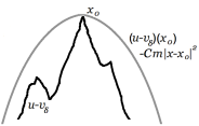
Figure 1. Illustration for Subsection 2.4.

Next, we consider the solution of the equation on $B_{r}(x_{0})$, but with “frozen” coefficients: let $\tilde{u}$ be the solution of

$$\left\{\begin{array}[]{l l}F(D^{2}\tilde{u},x_{0})=f(x_{0})&\quad\text{ in }B_{r}(x_{0}),\\ \tilde{u}=u&\quad\text{ on }\partial B_{r}(x_{0}).\end{array}\right.$$

Proposition 3.1 says $||u-\tilde{u}||_{L^{\infty}(B_{r}(x_{0}))}\leq Cr^{2+\alpha}$. Using this to estimate the right-hand side of (2.1) from above yields,

(2.2) $$Cmr^{2}\leq(\tilde{u}-v_{\delta})(x_{0})-\sup_{\partial B_{r}(x_{0})}(\tilde{u}-v_{\delta})+Cr^{2+\alpha}.$$

Since $\tilde{u}$ is the solution to a homogeneous equation, the regularity result Proposition 2.9, implies that $\tilde{u}$ has second order expansions with controlled error on large portions of $B_{r}(x_{0})$. As in [6], this extra regularity of $\tilde{u}$ allows us to compare $\tilde{u}$ and $v_{\delta}$ on $B_{r}(x_{0})$ and conclude

$$\sup_{B_{r}(x_{0})}(\tilde{u}-v_{\delta})-\sup_{\partial B_{r}(x_{0})}(\tilde{u}-v_{\delta})\leq r^{2}\delta^{\alpha}.$$

(This argument is Proposition 6.1). Using the previous estimate to bound the right-hand side of (2.2) from above yields,

$$Cmr^{2}\leq C\delta^{\alpha}r^{2}+Cr^{2+\alpha}.$$

Dividing by $r^{2}$ and choosing $r\leq\delta$ gives the desired estimate on $m$.

The main difference between the outline and the actual proof is that we need to work with inf- and sup- convolutions $v_{\delta}^{\theta,-}$ and $u^{\theta,+}$. Because we need take inf- and sup- convolutions inside of the small ball $B_{r}(x_{0})$, the radius $r$ has to be bigger than the parameter $\theta$ of the inf- and sup- convolutions. This restriction leads to problems. To get around them, we introduce the perturbations $F_{\varepsilon}$ and $F^{\varepsilon}$ of the equation itself. We define $F_{\varepsilon}$ and $F^{\varepsilon}$ by,

$$F_{\varepsilon}(X,x)=\inf_{y\in B_{\varepsilon}(x)\cap U}F(X,y),\ \text{ and }F^{\varepsilon}(X,x)=\sup_{y\in B_{\varepsilon}(x)\cap U}F(X,y).$$

We similarly define $f_{\varepsilon}$ and $f^{\varepsilon}$; please see Definition 4.1 for the details. We let $u_{\varepsilon}$ be the solution of,

$$\left\{\begin{array}[]{l l}F_{\varepsilon}(D^{2}u_{\varepsilon},x)=f^{\varepsilon}(x)&\quad\text{ in }U,\\ u_{\varepsilon}=g&\quad\text{ on }\partial U.\end{array}\right.$$

Proposition 4.2 asserts

$$||u_{\varepsilon}-u||_{L^{\infty}(U)}\leq C\varepsilon.$$

We take $\varepsilon\leq\delta^{\alpha}$ and replace $u$ with $u_{\varepsilon}$. According to the previous line, that the error we make is of size $C\varepsilon\leq C\delta^{\alpha}$, which does not affect the final estimate. Next, we “freeze the coefficients” of $F_{\varepsilon}$: we consider the solution $\tilde{u}_{\varepsilon}$ of

(2.3) $$\left\{\begin{array}[]{l l}F_{\varepsilon}(D^{2}\tilde{u}_{\varepsilon},x_{0})=f^{\varepsilon}(x_{0})&\quad\text{ in }B_{r}(x_{0}),\\ \bar{u}_{\varepsilon}=u_{\varepsilon}&\quad\text{ on }\partial B_{r}(x_{0}).\end{array}\right.$$

Then we proceed as explained in the first part of the outline. We do this for $\varepsilon\gg r$, so that the equation with frozen coefficients “sees” outside of $B_{r}(x_{0})$. This detail is extremely important and allows us to regularize using the inf- and sup- convolutions and complete the argument.

The proof of Theorem 1.4 follows essentially the same outline as the proof of Theorem 1.1. This because, as we show in Proposition 8.4, certain regularizations of the approximate solutions $v_{h}$ are $\delta$-solutions of (1.1).

3. The estimate between the solution of (1.1) and solutions of (1.1) with fixed coefficients.

In this section we establish the following result, which allows us to estimate the difference between $u$ and solutions of the equation with “frozen” coefficients:

Proposition 3.1.

Assume (U1), (F1), (F2), (G1), (G2) and $F(0,x)\equiv 0$. Let $u$ be the viscosity solution of (1.1). There exist a universal constant $\alpha$, a positive constant $r_{0}=r_{0}(\lambda,\Lambda,n,\kappa)$ and a positive constant $C$ that depends on $\lambda,\Lambda$, $n$, $\kappa$, $||f||_{C^{0,1}(U)}$, $||g||_{C^{1,\gamma}(\partial U)}$, $\operatorname{diam}U$ and the regularity of $\partial U$ such that if, we fix $r$ with $0<r<r_{0}$, a point $x_{0}$ such that $B_{r}(x_{0})\subset U$, and take $\tilde{u}$ to be the viscosity solution of

$$\left\{\begin{array}[]{l l}F(D^{2}\tilde{u},x_{0})=f(x_{0})&\quad\text{ in }B_{r}(x_{0}),\\ \tilde{u}=u&\quad\text{ on }\partial B_{r}(x_{0}),\end{array}\right.$$

then

$$||u-\tilde{u}||_{L^{\infty}(B_{r}(x_{0}))}\leq Cr^{2+\alpha}.$$

The proofs of Proposition 3.1 and Proposition 4.2, which we present in the next section, are similar to the proof of the comparison principle for uniformly elliptic equations of Ishii and Lions’ [9, Theorem III.1]. At the heart of the proof of both propositions is the following lemma, which combines Theorem 3.2 of [8] and Lemma III.1 of [9]. For the convenience of the reader, we give the statements of Theorem 3.2 of [8] and Lemma III.1 of [9] in Appendix A.

Lemma 3.2.

There exists a constant C(n) that depends only on $n$ such that the following holds. Assume $V$ is an open subset of $\mathbb{R}^{n}$ and $u,v\in C(V)$ are viscosity solutions of $F(D^{2}u,x)=f(x)$ and $G(D^{2}v,x)=g(x)$ in $V$. Suppose that $(x_{a},y_{a})\in V\times V$ is a local maximum of

(3.1) $$u(x)-v(y)-\frac{a}{2}|x-y|^{2}.$$

In addition, assume that there exist $s,t\in\mathbb{R}$ with

(3.2) $$t\leq\frac{\lambda}{2C(n)},$$

and such that

(3.3) $$\text{ for any $M,N\in\mathcal{S}_{n}$ with $M\leq N$, we have }F(M,x_{a})-G(N,y_{a})\leq t||M||+s-\lambda||N-M||.$$

Then,

(3.4) $$f(x_{a})-g(y_{a})-s\leq\frac{t^{2}C^{2}(n)a}{2\lambda}.$$

Proof.

We take $C(n)$ to be the constant from Lemma A.3. Since $(x_{a},y_{a})$ is an interior maximum of the quantity (3.1), Theorem A.2 implies that there exist $X,Y\in\mathcal{S}_{n}$ such that

(3.5) $$-3a\left(\begin{array}[]{cc}I&0\\ 0&I\\ \end{array}\right)\leq\left(\begin{array}[]{cc}X&0\\ 0&-Y\\ \end{array}\right)\leq 3a\left(\begin{array}[]{cc}I&-I\\ -I&I\\ \end{array}\right),$$

(3.6) $$F(X,x_{a})\geq f(x_{a}),$$

and

(3.7) $$G(Y,y_{a})\leq g(y_{a}).$$

Subtracting (3.7) from (3.6), we find

(3.8) $$f(x_{a})-g(y_{a})\leq F(X,x_{a})-G(Y,y_{a}).$$

We point out that the matrix inequality (3.5) implies $X\leq Y$. By assumption (3.3), we therefore have

$$F(X,x_{a})-G(Y,y_{a})\leq t||X||+s-\lambda||Y-X||.$$

We use (3.8) to bound the left-hand side of the previous line from below and find,

(3.9) $$f(x_{a})-g(x_{a})\leq t||X||+s-\lambda||Y-X||.$$

In addition, since $X$ and $Y$ satisfy (3.5), Lemma A.3 implies,

(3.10) $$||X||\leq C(n)\left\{a^{1/2}||X-Y||^{1/2}+||X-Y||\right\}.$$

We use (3.10) to bound the first term on the right-hand side of (3.9) from above and obtain,

$$f(x_{a})-g(x_{a})\leq tC(n)\left\{a^{1/2}||X-Y||^{1/2}+||X-Y||\right\}+s-\lambda||X-Y||.$$

Rearranging yields,

$$f(x_{a})-g(x_{a})-s\leq||X-Y||(tC(n)-\lambda)+tC(n)a^{1/2}||X-Y||^{1/2}.$$

According to the upper bound (3.2) on $t$, we have $tC(n)-\lambda\leq-\lambda/2$. We use this to estimate the first term on the right-hand side of the previous line from above, and find,

$$f(x_{a})-g(x_{a})-s\leq-\frac{\lambda}{2}||X-Y||+tC(n)a^{1/2}||X-Y||^{1/2},$$

Since the right-hand side is a quadratic polynomial in $z=||X-Y||^{1/2}$ with negative leading coefficient, we obtain

$$f(x_{a})-g(x_{a})-s\leq\sup_{z}\left\{-\frac{\lambda}{2}z^{2}+tC(n)a^{1/2}z\right\}=\frac{t^{2}C^{2}(n)a}{2\lambda},$$

as desired. ∎

For the proof of Proposition 3.1, we first rescale to a ball of radius 1, where we double variables and then apply Lemma 3.2. We will need to keep careful track of all the parameters once we double variables. In addition, in order to apply Lemma 3.2, we will need to verify that the point $(x_{a},y_{a})$ at which the supremum in (3.1) is achieved is contained in the interior of $V\times V$. For this, we need the following lemma. Its proof is elementary and is provided in Appendix A.

Lemma 3.3.

Suppose $v,w\in C^{0,1}(V)$ with $v=w$ on $\partial V$. Then, for all $a>0$,

$$\sup_{(\partial V\times V)\cup(V\times\partial V)}\left(v(x)-w(y)-\frac{a}{2}|x-y|^{2}\right)\leq 2(||Dv||_{L^{\infty}(V)}^{2}+||Dw||_{L^{\infty}(V)}^{2})a^{-1};$$

and, if $(x_{a},y_{a})\in V\times V$ is a point at which the supremum on the left-hand side of the previous line is achieved, then

$$|x_{a}-y_{a}|\leq 2a^{-1}\min\{||Du||_{L^{\infty}(V)},||Dv||_{L^{\infty}(V)}\}.$$

We proceed with:

Proof of Proposition 3.1.

We will establish the estimate

$$\sup_{B_{r}}\left(u-\tilde{u}\right)\leq Cr^{2+\alpha};$$

the proof of the estimate on $\sup_{B_{r}}\left(\tilde{u}-u\right)$ is similar. Throughout this proof we will use $C_{i}$ with $i=1,2,...$ to denote generic constants that may depend on $\lambda$, $\Lambda$, $n$, $\kappa$, $||f||_{L^{\infty}(U)}$, $||g||_{C^{1,\alpha}(\partial U)}$, $\operatorname{diam}U$ and the regularity of $\partial U$. We take $\alpha$ to be the exponent given by Proposition 2.5 and $C(n)$ to be the constant from Lemma 3.2. We define the constants $r_{0}$ and $\theta_{0}$ by

$$r_{0}=\min\left\{\frac{\lambda}{2\kappa C(n)},1\right\}$$

and

$$\theta_{0}=\frac{2C(n)^{2}\kappa^{2}}{\lambda}.$$

We take $0<r\leq r_{0}$. We define the parameter $\theta$ by,

$$\theta=\theta_{0}+r^{1-\alpha}||Df||_{L^{\infty}(U)}+r^{1-\alpha}\kappa,$$

and the function $\bar{u}$ to be the solution of

(3.11) $$\left\{\begin{array}[]{l l}F(D^{2}\bar{u},x_{0})=f(x_{0})-\theta r^{\alpha}&\quad\text{ in }B_{r}(x_{0}),\\ \bar{u}=u&\quad\text{ on }\partial B_{r}(x_{0}).\end{array}\right.$$

Next, for $y\in B_{1}$, we define the rescaled functions $u^{r}$ and $\bar{u}^{r}$ by,

(3.12) $$u^{r}(y)=\frac{u(yr+x_{0})-u(x_{0})-Du(x_{0})\cdot(yr)}{r^{1+\alpha}}$$

and

(3.13) $$\bar{u}^{r}(y)=\frac{\bar{u}(yr+x_{0})-u(x_{0})-Du(x_{0})\cdot(yr)}{r^{1+\alpha}}.$$

We denote by $\tilde{F}$ the rescaled nonlinearity,

$$\tilde{F}(X,y)=r^{1-\alpha}F(r^{\alpha-1}X,ry+x_{0}),$$

and define $\tilde{f}(y)=r^{1-\alpha}f(ry+x_{0})$. The nonlinearity $\tilde{F}$ is uniformly elliptic with the same ellipticity constants as $F$. Moreover, since $F$ satisfies (F2), we have, for any $y_{1}$ and $y_{2}$ in $B_{1}$,

(3.14) $$|\tilde{F}(X,y_{1})-\tilde{F}(X,y_{2})|\leq\kappa(r||X||+r^{2-\alpha}).$$

In addition, we have the following estimate on $D\tilde{f}$, which follows simply from the definition of $\tilde{f}$:

(3.15) $$||D\tilde{f}||_{L^{\infty}(B_{1})}=r^{2-\alpha}||Df||_{L^{\infty}(B_{r}(x_{0}))}\leq r^{2-\alpha}||Df||_{L^{\infty}(U)}.$$

The definitions of $\tilde{F}$, $\tilde{f}$, $u^{r}$ and $\bar{u}^{r}$ imply that $u^{r}$ is a solution of

$$\tilde{F}(D^{2}u^{r},y)=\tilde{f}(y)\text{ in }B_{1},$$

and that $\bar{u}^{r}(x)$ is a solution of

(3.16) $$\left\{\begin{array}[]{l l}\tilde{F}(D^{2}\bar{u}^{r},0)=\tilde{f}(0)-\theta r&\quad\text{ in }B_{1},\\ \bar{u}^{r}=u^{r}&\quad\text{ on }\partial B_{1}.\end{array}\right.$$

We claim

(3.17) $$\sup_{B_{1}}(u^{r}-\bar{u}^{r})\leq 4(||D\bar{u}^{r}||_{L^{\infty}(B_{1})}^{2}+||Du^{r}||_{L^{\infty}(B_{1})}^{2})r,$$

which we will prove by contradiction. To this end, we assume,

(3.18) $$\sup_{B_{1}}(u^{r}-\bar{u}^{r})>4(||D\bar{u}^{r}||_{L^{\infty}(B_{1})}^{2}+||Du^{r}||_{L^{\infty}(B_{1})}^{2})r.$$

We double variables and consider

(3.19) $$\sup_{x,y\in B_{1}}\left(u^{r}(x)-\bar{u}^{r}(y)-\frac{r^{-1}}{2}|x-y|^{2}\right).$$

The quantity in the previous line is larger than the difference between $u^{r}(x)$ and $\bar{u}^{r}(x)$ for any $x$ in $B_{1}$; hence,

$$\sup_{x,y\in B_{1}}\left(u^{r}(x)-\bar{u}^{r}(y)-\frac{r^{-1}}{2}|x-y|^{2}\right)\geq\sup_{B_{1}}(u^{r}-\bar{u}^{r}).$$

Next, we use (3.18) to bound the right-hand side of the previous line from below and obtain,

$$\sup_{x,y\in B_{1}}\left(u^{r}(x)-\bar{u}^{r}(y)-\frac{r^{-1}}{2}|x-y|^{2}\right)>4(||D\bar{u}^{r}||_{L^{\infty}(B_{1})}^{2}+||Du^{r}||_{L^{\infty}(B_{1})}^{2})r.$$

Let us denote by $(x_{r},y_{r})$ a point in $\bar{B}_{1}\times\bar{B_{1}}$ where the supremum is achieved in (3.19). The previous line, together with Lemma 3.3 applied with $V=B_{1}$ and $a=r^{-1}$, implies $(x_{r},y_{r})\in B_{1}\times B_{1}$. In other words, $(x_{r},y_{r})$ is an interior maximum of the quantity (3.19).

We will apply now Lemma 3.2 with $a=r^{-1}$ and with $B_{1}$, $\tilde{F}(M,x)$, $\tilde{F}(M,0)$, $\tilde{f}$, and $\tilde{f}(0)-\theta r$ instead of $V$, $F$, $G$, $f$, and $g$, respectively. We have just shown that $(x_{r},y_{r})\in B_{1}\times B_{1}$. We now take

$$t=\kappa r\text{ and }s=\kappa r^{2-\alpha}$$

and verify the two remaining hypotheses of Lemma 3.2. Our choice of $r\leq r_{0}$ implies that $t$ satisfies (3.2). Let us now first verify that (3.3) holds: assume $M,N\in\mathcal{S}_{n}$ with $M\leq N$. Then, by (3.14) and the uniform ellipticity of $\tilde{F}$, we find

$$\tilde{F}(M,x_{r})-\tilde{F}(N,0) \leq\tilde{F}(M,0)+\kappa r||X||+\kappa r^{2-\alpha}-\tilde{F}(N,0)$$

$$\leq\kappa r||X||+\kappa r^{2-\alpha}-\lambda||N-M||.$$

Thus (3.3) is satisfied. Hence, with our choices of $t$ and $s$, the conclusion (3.4) of Lemma 3.2 yields,

(3.20) $$\tilde{f}(x_{r})-(\tilde{f}(0)-\theta r)-\kappa r^{2-\alpha}\leq\frac{t^{2}C^{2}(n)r^{-1}}{2\lambda}=\frac{\kappa^{2}rC^{2}(n)}{2\lambda}.$$

Since $x_{r}\in B_{1}$ and $f$ is Lipschitz, we may estimate the difference of the first two terms of the left-hand side of (3.20) by,

$$\tilde{f}(x_{r})-\tilde{f}(0)\geq-||D\tilde{f}||_{L^{\infty}(B_{1})}\geq-r^{2-\alpha}||Df||_{L^{\infty}(U)},$$

where the second inequality follows from (3.15). We use the previous line to estimate the left-hand side of (3.20) from below and obtain,

$$-r^{2-\alpha}||Df||_{L^{\infty}(U)}+\theta r-\kappa r^{2-\alpha}\leq\frac{\kappa^{2}rC^{2}(n)}{2\lambda}.$$

We use the definition of $\theta$ to rewrite the second term on the left-hand side, and find,

$$-r^{2-\alpha}||Df||_{L^{\infty}(U)}+r(\theta_{0}+r^{1-\alpha}||Df||_{L^{\infty}(U)}+r^{1-\alpha}\kappa)-\kappa r^{2-\alpha}\leq\frac{\kappa^{2}rC^{2}(n)}{2\lambda}.$$

We notice that the left-hand side is simply $\theta_{0}r$. Thus, the previous line reads,

$$\theta_{0}r\leq\frac{C(n)^{2}\kappa^{2}}{\lambda}r,$$

which is impossible, since $r$ is positive and we chose $\theta_{0}=2\frac{C(n)^{2}\kappa^{2}}{\lambda}$. We have obtained the desired contradiction; therefore, (3.17) must hold. In order to complete the proof of the proposition, it is now left to bound the terms $||D\bar{u}^{r}||_{L^{\infty}(B_{1})}$ and $||Du^{r}||_{L^{\infty}(B_{1})}$ that appear on the right-hand side of (3.17) and to “undo” the rescaling. To this end, from the definition of $u^{r}$, we see

(3.21) $$||u^{r}||_{C^{1,\alpha}(B_{1})}=||u||_{C^{1,\alpha}(B_{r}(x_{0}))}\leq||u||_{C^{1,\alpha}(U)}\leq C_{2},$$

where the second inequality follows from Proposition 2.5. Since $\bar{u}^{r}$ is the solution of (3.16), Proposition 2.5 applied to $\bar{u}^{r}$ in $B_{1}$ implies that there exists $C>0$ that depends on $n,\lambda,\Lambda$ and $\kappa$ such that

$$||\bar{u}^{r}||_{C^{1,\alpha}(B_{1})}\leq C(||\tilde{f}||_{L^{\infty}(B_{1})}+\theta r+||u^{r}||_{C^{1,\alpha}(B_{1})})=C(r^{1-\alpha}||f||_{L^{\infty}(B_{r}(x_{0}))}+\theta r+C_{2}),$$

where the equality follows since $||\tilde{f}||_{L^{\infty}(B_{1})}=r^{1-\alpha}||f||_{L^{\infty}(B_{r}(x_{0}))}$ and from the estimate (3.21) on $||u^{r}||_{C^{1,\alpha}(B_{1})}$. The two previous estimates imply,

$$||D\bar{u}^{r}||_{L^{\infty}(B_{1})}^{2}+||Du^{r}||_{L^{\infty}(B_{1})}^{2}\leq C_{3}.$$

We use this to bound the right-hand side of (3.17) from above and obtain

(3.22) $$\sup_{B_{1}}(u^{r}-\bar{u}^{r})\leq C_{3}r.$$

We have defined $\bar{u}^{r}$ and $u^{r}$ by, respectively, (3.13) and (3.12). Thus, subtracting (3.13) from (3.12) yields, for all $y\in B_{1}$,

$$u^{r}(y)-\bar{u}^{r}(y)=\frac{1}{r^{1+\alpha}}\left(u(yr+x_{0})-\bar{u}(yr+x_{0})\right).$$

Therefore, the left-hand side of (3.22) is exactly $r^{-(1+\alpha)}\sup_{B_{r}(x_{0})}(u-\bar{u})$, so we have,

$$\frac{1}{r^{1+\alpha}}\sup_{B_{r}(x_{0})}(u-\bar{u})\leq C_{3}r.$$

Upon multiplying both sides by $r^{1+\alpha}$ we find,

(3.23) $$\sup_{B_{r}(x_{0})}(u-\bar{u})\leq C_{3}r^{2+\alpha}.$$

It is left to “replace” $\bar{u}$ by $\tilde{u}$. For this we employ Lemma 2.6 in $B_{r}$ with $c=\theta r^{\alpha}$. We obtain,

$$\sup_{B_{r}(x_{0})}(\bar{u}-\tilde{u})\leq\frac{\theta r^{2+\alpha}}{2\lambda}.$$

Together with the estimate (3.23), we find

$$\sup_{B_{r}(x_{0})}(u-\tilde{u}) \leq\sup_{B_{r}(x_{0})}(u-\bar{u})+\sup_{B_{r}(x_{0})}(\bar{u}-\tilde{u})$$

$$\leq C_{3}r^{2+\alpha}+\frac{\theta r^{2+\alpha}}{2\lambda}=C_{4}r^{2+\alpha},$$

thus completing the proof of the proposition. ∎

The following Corollary follows directly from Proposition 3.1, Proposition 2.4 and Proposition 2.5.

Corollary 3.4.

Assume (U1), (F1), (F2), (G1), (G2) and $F(0,x)\equiv 0$. Assume $u$ is the viscosity solution of (1.1). There exists a universal constant $\alpha$ and positive constants $r_{0}=r_{0}(n,\lambda,\Lambda,\kappa)$ and $C$ that depends on $n$, $\lambda$, $\Lambda$, $\kappa$, $\operatorname{diam}U$, $||f||_{C^{0,1}(U)}$, the regularity of $\partial{U}$ and $||g||_{C^{1,\gamma}(\partial U)}$, such that, if $\tilde{u}$ is the viscosity solution of

$$\left\{\begin{array}[]{l l}F(D^{2}\tilde{u},x_{0})=f(x_{0})&\quad\text{ in }B_{2r}(x_{0}),\\ \tilde{u}(x)=u(x)&\quad\text{ for }x\in\partial B_{2r}(x_{0}),\end{array}\right.$$

then

$$||\tilde{u}||_{C^{1,\alpha}(B_{r}(x_{0}))}^{*}\leq C$$

and

$$||\tilde{u}-u||_{L^{\infty}(B_{2r}(x_{0}))}\leq Cr^{2+\alpha}.$$

4. Perturbations of the nonlinearity

Let us state precisely the definitions of the two perturbations of the nonlinearity $F$ that we mentioned in Section 2.4.

Definition 4.1.

For $F(X,x)\in C(\mathcal{S}_{n}\times U)$ and $\varepsilon>0$, we define $F_{\varepsilon}$ and $F^{\varepsilon}$ by,

$$F_{\varepsilon}(X,x)=\inf_{y\in B_{\varepsilon}(x)\cap U}F(X,y),\ \text{ and }F^{\varepsilon}(X,x)=\sup_{y\in B_{\varepsilon}(x)\cap U}F(X,y).$$

For $f\in C(U)$ and $\varepsilon>0$, we define $f_{\varepsilon}$ and $f^{\varepsilon}$ by

$$f_{\varepsilon}(x)=\inf_{y\in B_{\varepsilon}(x)\cap U}f(y),\ \text{ and }f^{\varepsilon}(x)=\sup_{y\in B_{\varepsilon}(x)\cap U}f(y).$$

We observe that if $F$ satisfies (F1) and (F2), then so do $F_{\varepsilon}$ and $F^{\varepsilon}$. Our use of these perturbations is inspired by [13, Theorem 2.1], a proof of the existence of $C^{2,\alpha}$ approximate solutions for convex equations, which is a key step in Krylov’s analysis of the convex/concave case.

This section is devoted to the proof of:

Proposition 4.2.

Assume that $u$ and $u_{\varepsilon}$ are the viscosity solution of, respectively, (1.1) and

(4.1) $$\left\{\begin{array}[]{l l}F_{\varepsilon}(D^{2}u_{\varepsilon},x)=f^{\varepsilon}(x)&\quad\text{ in }U,\\ u_{\varepsilon}=g&\quad\text{ on }\partial U.\end{array}\right.$$

There exist positive constants $\varepsilon_{0}$ and $C$ that depend on $n$, $\lambda$, $\Lambda$, $\kappa$, $||g||_{C^{1,\gamma}(\partial U)}$, $||f||_{C^{0,1}(U)}$, $\operatorname{diam}U$ and the regularity of $\partial U$ such that for $\varepsilon\leq\varepsilon_{0}$, and for all $x\in U$,

$$0\leq u(x)-u_{\varepsilon}(x)\leq C\varepsilon.$$

A similar statement holds for $F^{\varepsilon}$ and $f_{\varepsilon}$ instead of $F_{\varepsilon}$ and $f^{\varepsilon}$, except there the conclusion is,

$$0\leq u_{\varepsilon}(x)-u(x)\leq C\varepsilon.$$

The proof of Proposition 4.2 is similar to the proof Proposition 3.1 – the key is the application of Lemma 3.2.

Proof of Proposition 4.2.

The definitions of $F_{\varepsilon}$ and $f^{\varepsilon}$ imply that $u_{\varepsilon}$ is a subsolution of (1.1). Therefore, we have $u_{\varepsilon}\leq u$ for all $\varepsilon$. The remainder of the proof is devoted to establishing an upper bound on $u-u_{\varepsilon}$.

By Proposition 2.5, there exists a constant $\bar{C}$ that depends on $\lambda$, $\Lambda$, $\kappa$, $\operatorname{diam}U$ and the regularity of $\partial U$ such that

(4.2) $$||Du||_{L^{\infty}(U)}\leq\bar{C}(||g||_{C^{1,\gamma}(\partial U)}+||f||_{L^{\infty}(U)}).$$

Let $C(n)$ be the constant from Lemma 3.2. We define the constant $\varepsilon_{0}$ by

$$\varepsilon_{0}=\frac{\lambda}{2\kappa C(n)(2\bar{C}(||g||_{C^{1,\gamma}(\partial U)}+||f||_{L^{\infty}(U)})+1)},$$

We remark that $\varepsilon_{0}$ does not depend on $u$, and, according to (4.2), satisfies,

(4.3) $$\varepsilon_{0}\leq\frac{\lambda}{2\kappa C(n)(2||Du||_{L^{\infty}(U)}+1)}.$$

We fix $\varepsilon\leq\varepsilon_{0}$ and introduce the parameters $\theta_{0}$ and $\theta$:

$$\theta_{0}=\varepsilon\frac{\kappa^{2}(2||Du||_{L^{\infty}(U)}+1)^{2}}{\lambda}$$

and

$$\theta=\theta_{0}+\varepsilon(\kappa+||Df||_{L^{\infty}(U)})(2||Du||_{L^{\infty}(U)}+1).$$

We define $\tilde{u}_{\varepsilon}$ to be the viscosity solution of

$$\left\{\begin{array}[]{l l}F_{\varepsilon}(D^{2}\tilde{u}_{\varepsilon},x)=f^{\varepsilon}(x)-\theta&\quad\text{ in }U,\\ \tilde{u}_{\varepsilon}=g&\quad\text{ on }\partial U.\end{array}\right.$$

We claim,

(4.4) $$\sup_{U}(u-\tilde{u}_{\varepsilon})\leq 4(||D\tilde{u}_{\varepsilon}||_{L^{\infty}(U)}^{2}+||Du||_{L^{\infty}(U)}^{2})\varepsilon,$$

which we will prove by contradiction. To this end, we assume that (4.4) does not hold, so that instead we have,

(4.5) $$\sup_{U}(u-\tilde{u}_{\varepsilon})>4(||D\tilde{u}_{\varepsilon}||_{L^{\infty}(U)}^{2}+||Du||_{L^{\infty}(U)}^{2})\varepsilon.$$

We double variables and consider

(4.6) $$\sup_{x,y\in U}\left(u(x)-\tilde{u}_{\varepsilon}(y)-\varepsilon^{-1}\frac{|x-y|^{2}}{2}\right).$$

We have that the quantity in the previous line is greater than the supremum in $x$ of $u(x)-\tilde{u}_{\varepsilon}(x)$:

$$\sup_{x,y\in U}\left(u(x)-\tilde{u}_{\varepsilon}(y)-\frac{1}{\varepsilon}\frac{|x-y|^{2}}{2}\right)\geq\sup_{U}(u-\tilde{u}_{\varepsilon}).$$

We use (4.5) to bound the right-hand side of the previous line from below and obtain,

$$\sup_{x,y\in U}\left(u(x)-\tilde{u}_{\varepsilon}(y)-\frac{1}{\varepsilon}\frac{|x-y|^{2}}{2}\right)\geq 4(||D\tilde{u}_{\varepsilon}||_{L^{\infty}(U)}^{2}+||Du||_{L^{\infty}(U)}^{2})\varepsilon.$$

Let us denote by $(x_{\varepsilon},y_{\varepsilon})$ a point where the supremum is achieved in the quantity (4.6). Together with the previous line, Lemma 3.3 applied with $a=\varepsilon^{-1}$ implies that $x_{\varepsilon}$ and $y_{\varepsilon}$ are both contained in the interior of $U$.

We will apply Lemma 3.2 with $a=\varepsilon^{-1}$, and $F_{\varepsilon}$ and $(f^{\varepsilon}(x)-\theta)$ instead of $G$ and $g(x)$. It is left to chose the parameters $t$ and $s$ appropriately and verify the remaining hypotheses of Lemma 3.2. To this end, let $M,N\in\mathcal{S}_{n}$ be such that $M\leq N$. We denote by $y_{\varepsilon}^{*}$ a point where the supremum is achieved in the definition of $F_{\varepsilon}(N,y_{\varepsilon}^{*})$. In particular, we have

(4.7) $$|y_{\varepsilon}^{*}-y_{\varepsilon}|\leq\varepsilon.$$

We use the definition of $y_{\varepsilon}^{*}$ and the property (F2) of $F$ to find,

$$F(M,x_{\varepsilon})-F_{\varepsilon}(N,y_{\varepsilon}) =F(M,x_{\varepsilon})-F(N,y_{\varepsilon}^{*})$$

$$\leq F(M,y_{\varepsilon}^{*})+\kappa|x_{\varepsilon}-y_{\varepsilon}^{*}|(||M||+1)-F(N,y_{\varepsilon}^{*}).$$

We use our assumption $M\leq N$ and the uniform ellipticity of $F$ to bound the right-hand side of the previous line from above and obtain,

(4.8) $$F(M,x_{\varepsilon})-F_{\varepsilon}(N,y_{\varepsilon})\leq\kappa|x_{\varepsilon}-y_{\varepsilon}^{*}|(||M||+1)-\lambda||N-M||.$$

We will now estimate $|x_{\varepsilon}-y_{\varepsilon}^{*}|$. According to the triangle inequality, Lemma 3.3 and the estimate (4.7), we have

(4.9) $$|x_{\varepsilon}-y_{\varepsilon}^{*}|\leq|x_{\varepsilon}-y_{\varepsilon}|+|y_{\varepsilon}-y_{\varepsilon}^{*}|\leq 2\varepsilon||Du||_{L^{\infty}(U)}+\varepsilon=\varepsilon(2||Du||_{L^{\infty}(U)}+1).$$

We set $s$ and $t$ to be,

$$s=t=\varepsilon\kappa(2||Du||_{L^{\infty}(U)}+1).$$

Together with the estimate (4.9), this implies,

$$|x_{\varepsilon}-y_{\varepsilon}^{*}|\leq t\kappa^{-1}=s\kappa^{-1}.$$

We use the previous line to bound from above the first term on the right-hand side of (4.8) and obtain,

$$F(M,x_{\varepsilon})-F_{\varepsilon}(N,y_{\varepsilon})\leq t||M||+s-\lambda||N-M||.$$

And, by our choice of $\varepsilon\leq\varepsilon_{0}$, we have that $t$ satisfies (3.2). Thus, the hypotheses (3.3) and (3.2) of Lemma 3.2 are satisfied, and we obtain that (3.4) holds. In our situation, (3.4) reads,

(4.10) $$f(x_{\varepsilon})-(f^{\varepsilon}(y_{\varepsilon})-\theta)-\varepsilon\kappa(2||Du||_{L^{\infty}(U)}+1)\leq\frac{t^{2}C^{2}(n)\varepsilon^{-1}}{2\lambda}=\frac{\varepsilon\kappa^{2}(2||Du||_{L^{\infty}(U)}+1)^{2}}{2\lambda},$$

where the equality follows by our choice of $t$. Next we will use that $f$ is Lipschitz to bound the left-hand side of (4.10) from below. We denote by $y_{\varepsilon}^{+}$ a point where the supremum is achieved in the definition of $f^{\varepsilon}(y_{\varepsilon})$. We have,

(4.11) $$|y_{\varepsilon}^{+}-y_{\varepsilon}|\leq\varepsilon.$$

According to the triangle inequality, the estimate on $|x_{\varepsilon}-y_{\varepsilon}|$ of Lemma 3.3, and (4.11), we have

(4.12) $$|x_{\varepsilon}-y_{\varepsilon}^{+}|\leq|x_{\varepsilon}-y_{\varepsilon}|+|y_{\varepsilon}-y_{\varepsilon}^{+}|\leq 2\varepsilon||Du||_{L^{\infty}(U)}+\varepsilon=\varepsilon(2||Du||_{L^{\infty}(U)}+1).$$

Since $f$ is Lipschitz, we find

(4.13) $$f(x_{\varepsilon})-f^{\varepsilon}(y_{\varepsilon})=f(x_{\varepsilon})-f(y_{\varepsilon}^{+})\geq-||Df||_{L^{\infty}(U)}|x_{\varepsilon}-y_{\varepsilon}^{+}|\geq-\varepsilon||Df||_{L^{\infty}(U)}(2||Du||_{L^{\infty}(U)}+1),$$

where the second inequality follows from (4.12). We use the previous line to estimate the left-hand side of (4.10) from below and find,

$$-\varepsilon||Df||_{L^{\infty}(U)}(2||Du||_{L^{\infty}(U)}+1))+\theta-\varepsilon\kappa(2||Du||_{L^{\infty}(U)}+1)\leq\frac{\varepsilon\kappa^{2}(2||Du||_{L^{\infty}(U)}+1)^{2}}{2\lambda},$$

which, upon rearranging the left-hand side becomes,

$$\theta-(\varepsilon||Df||_{L^{\infty}(U)}+\kappa)(2||Du||_{L^{\infty}(U)}+1)\leq\frac{\varepsilon\kappa^{2}(2||Du||_{L^{\infty}(U)}+1)^{2}}{2\lambda}.$$

According to the definition of the parameter $\theta$, the left-hand side of the previous line is simply $\theta_{0}$. Hence we obtain,

$$\theta_{0}\leq\frac{\varepsilon\kappa^{2}(2||Du||_{L^{\infty}(U)}+1)^{2}}{2\lambda},$$

which contradicts our choice of $\theta_{0}$. Therefore (4.4) holds. We use Proposition (2.5) to bound the right-hand side of (4.4) from above, and find, for some constant $C$ that depends on $n,\lambda,\kappa$, $||g||_{C^{1,\gamma}(U)}$, $\operatorname{diam}U$ and the regularity of $\partial U$,

(4.14) $$\sup_{U}(u-\tilde{u}_{\varepsilon})\leq C\varepsilon.$$

Let us now “replace” $\tilde{u}_{\varepsilon}$ by $u_{\varepsilon}$. We will emply Lemma 2.6 with $c=\theta$. We find,

(4.15) $$\sup_{U}(\tilde{u}_{\varepsilon}-u_{\varepsilon})\leq\frac{(\operatorname{diam}U)^{2}\theta}{2\lambda}.$$

From (4.14), (4.15), and the definitions of $\theta$ and $\theta_{0}$, we conclude

$$\sup_{U}(u-u_{\varepsilon})\leq\sup_{U}(u-\tilde{u}_{\varepsilon})+\sup_{U}(\tilde{u}_{\varepsilon}-u_{\varepsilon})\leq\sup_{U}(u-\tilde{u}_{\varepsilon})+\frac{(\operatorname{diam}U)^{2}\theta}{2\lambda}\leq\varepsilon C,$$

where $C$ depends on $n,\lambda,\kappa$, $||Df||_{L^{\infty}(U)}$, $||g||_{C^{1,\gamma}(U)}$, $\operatorname{diam}U$ and the regularity of $\partial U$. ∎

5. An elementary lemma

In this section we establish an elementary lemma that plays an important role in the proof of our main result.

Lemma 5.1.

Assume $w\in C^{0,\eta}(U)$ is such that $w\leq 0$ on $\partial U$ and $\sup_{U}w>0$. Then for any positive $m$ with $m\leq\sup_{U}w$, there exists $x_{0}\in U$ with

(5.1) $$d(x_{0},\partial U)\geq\left(\frac{m}{2[w]_{C^{0,\eta}(U)}}\right)^{1/\eta}$$

and an affine function $l(x)$ with $l(x_{0})=w(x_{0})$ and

(5.2) $$w(x)\leq l(x)-\frac{m}{2(\operatorname{diam}U)^{2}}|x-x_{0}|^{2}$$

for all $x\in U$.

Proof.

Let $w\in C^{0,\eta}(U)$ be as in the statement of the lemma, and let us take $m$ with

$$m\leq\sup_{U}w.$$

Let us use $R$ to denote $R=\operatorname{diam}U$. We fix some $y\in U$. The function

(5.3) $$x\mapsto-\frac{m}{2R^{2}}|x-y|^{2}-w(x)$$

achieves its minimum on $\bar{U}$ at some $x_{0}\in\bar{U}$. (We point out that $x_{0}$ is a point where $w$ is touched from above by a concave paraboloid of opening $\frac{m}{2R^{2}}$.) Thus, for all $x\in U$, we have

$$w(x_{0}) \geq w(x)+\frac{m}{2R^{2}}|x-y|^{2}-\frac{m}{2R^{2}}|x_{0}-y|^{2}$$

$$\geq w(x)-\frac{m}{2R^{2}}|x_{0}-y|^{2}.$$

We take the supremum over $x\in U$ of both sides and obtain,

$$w(x_{0})\geq\sup_{x\in U}w(x)-\frac{m}{2R^{2}}|x_{0}-y|^{2}.$$

The definition of $R$ implies $|x_{0}-y|^{2}\leq R^{2}$. We use this, and that we have $m\leq\sup_{U}w$, to estimate the right-hand side of the previous line from below. We obtain,

(5.4) $$w(x_{0})\geq m-\frac{m}{2}=\frac{m}{2}.$$

Since $w\in C^{0,\eta}(U)$ and $w\leq 0$ on $\partial U$, we obtain an upper bound on $w(x_{0})$ in terms of the distance between $x_{0}$ and the boundary of $U$:

$$w(x_{0})\leq d(x_{0},\partial U)^{\eta}[w]_{C^{0,\eta}(U)}.$$

We use this to bound the left-hand side of (5.4) from above and obtain,

$$d(x_{0},\partial U)^{\eta}[w]_{C^{0,\eta}(U)}\geq\frac{m}{2},$$

and so the estimate (5.1) follows.

Let us now establish (5.2). Since $x_{0}$ is a minimum of the map (5.3), we have that for all $x\in U$,

$$w(x) \leq w(x_{0})+\frac{m}{2R^{2}}\left(|x_{0}-y|^{2}-|x-y|^{2}\right).$$

We have $|x-y|^{2}=|x-x_{0}|^{2}+2\langle x-x_{0},x_{0}-y\rangle+|x_{0}-y|^{2}$, so we find,

$$w(x) \leq w(x_{0})+\frac{m}{2R^{2}}\left(-|x_{0}-x|^{2}-2\langle x-x_{0},x_{0}-y\rangle\right),$$

which yields (5.2) upon setting $l(x)=w(x_{0})-\frac{m}{R^{2}}\langle x-x_{0},x_{0}-y\rangle$. ∎

6. A key estimate between solutions and sufficiently regular $\delta$-solutions

In this section we state and prove Proposition 6.1, a key part of the proofs of the two main results, Theorems 1.1 and 1.4. Roughly, Proposition 6.1 says that if $w$, $u$ and $v$ are, respectively, a $\delta$-subsolution, a solution and a $\delta$-supersolution on a ball of radius $2r$ and satisfy,

$$w\leq u\leq v$$

on the boundary of the ball of radius $r/2$, then we have

$$w-\tilde{c}\delta^{\tilde{\alpha}}r^{2}\leq u\leq v+\tilde{c}\delta^{\tilde{\alpha}}r^{2},$$

on the interior of the ball of radius $r/2$. The key ingredient in the proof is Proposition 2.9; the main difficulty is that we assume $w$, $u$ and $v$ satisfy different equations. In particular, $u$ satisfies an equation with frozen coefficients. We introduce the constants

$$\zeta=\frac{2\sigma}{12\sigma+9n},\ \ \theta=\frac{\zeta}{4(2-\alpha)},\ \ \alpha_{1}=\frac{\zeta}{4},$$

where $\sigma$ is the exponent from Proposition 2.9 and $\alpha$ is the exponent from Proposition 2.5. We remark that since $\sigma$ and $\alpha$ are universal, then so are $\zeta$, $\theta$, and $\alpha_{1}$.

Proposition 6.1.

Assume (F1), (F2), and $F(0,x)\equiv 0$. Suppose $x_{0}\in U$ and $C_{1}$ and $\nu$ are positive constants. For $\delta>0$, we define the quantities $r$ and $\varepsilon$ by

$$r=\delta^{\theta},\text{ and }\varepsilon=\nu+\delta^{\theta}=\nu+r.$$

There exist a universal constant $\tilde{\alpha}$ and positive constants $\tilde{c}$, $\tilde{\delta}$ that depend on $C_{1}$, $n$, $\lambda$, and $\Lambda$ such that if $\delta\leq\tilde{\delta}$ and,

1. if $v$ is a $\delta$-supersolution of

   (6.1) $$F_{\nu}(D^{2}v,x)=f^{\nu}(x)\text{ in }B_{2r}(x_{0})$$

   and $\tilde{u}_{\varepsilon}$ is a viscosity solution of

   (6.2) $$F_{\varepsilon}(D^{2}\tilde{u}_{\varepsilon},x_{0})=f^{\varepsilon}(x)\text{ in }B_{2r}(x_{0})$$

   that satisfy

   1. $\displaystyle||\tilde{u}_{\varepsilon}||_{C^{1,\alpha}(B_{r}(x_{0}))}^{*}\leq C_{1}$,

   2. $\displaystyle D^{2}v(x)\leq\delta^{-\zeta}I$ in the sense of distributions for all $x\in B_{2r}(x_{0})$, and

   3. $\displaystyle\sup_{\partial B_{r/2}(x_{0})}(\tilde{u}_{\varepsilon}-v)\leq 0$,

   then

   (6.3) $$\sup_{B_{r/2}(x_{0})}(\tilde{u}_{\varepsilon}-v)\leq\tilde{c}\delta^{\tilde{\alpha}}r^{2};$$

2. if $w$ is a $\delta$-subsolution of $F^{\nu}(D^{2}w,x)=f_{\nu}(x)$ in $B_{2r}(x_{0})$ and $\tilde{u}^{\varepsilon}$ a solution of $F^{\varepsilon}(D^{2}\tilde{u}^{\varepsilon},x_{0})=f_{\varepsilon}(x_{0})$ in $B_{2r}(x_{0})$ that satisfy $||\tilde{u}^{\varepsilon}||_{C^{1,\alpha}(B_{r}(x_{0}))}^{*}\leq C_{1}$, $D^{2}w(x)\geq-\delta^{-\zeta}I$ in the sense of distributions for all $x\in B_{2r}(x_{0})$, and $\sup_{\partial B_{r/2}(x_{0})}(w-\tilde{u}^{\varepsilon})\leq 0$, then,

   $$\sup_{B_{r/2}(x_{0})}(w-\tilde{u}^{\varepsilon})\leq\tilde{c}\delta^{\tilde{\alpha}}r^{2}.$$

6.1. Outline of the proof of Proposition 6.1

We outline the proof of the first part of Proposition 6.1; the proof of the second part is very similar. The main idea is to control the supremum of $(\tilde{u}_{\varepsilon}-v)$ by the size of the contact set of $(\tilde{u}_{\varepsilon}-v)$ with its concave envelope.

We regularize $\tilde{u}_{\varepsilon}$ by sup-convolution. Then we subtract a small quadratic in order to obtain a strict subsolution of (6.2). Let us denote the resulting function by $\bar{u}$. The assumptions (1c) and (1b) imply that $\bar{u}$ and $v$ satisfy the hypotheses of Proposition 2.3, so we find,

$$\sup(\bar{u}-v)\leq Cr\left(\int_{\{\bar{u}-v=\Gamma_{\bar{u}-v}\}}|\det D^{2}\Gamma_{\bar{u}-v}|\right)^{\frac{1}{n}}.$$

We proceed by contradiction and assume $\sup(\bar{u}-v)$ is “large”. The previous estimate, together with an upper bound on $|\det D^{2}\Gamma_{\bar{u}-v}|$, thus implies that the contact set $\{\bar{u}-v=\Gamma_{\bar{u}-v}\}$ is “large” as well.

The key part of our argument is Proposition 2.9, which says that there is a set $A_{t}^{+}$ on which $\bar{u}$ is very close to being a paraboloid. Moreover, Proposition 2.9 provides a lower bound on the size of this good set $A_{t}^{+}$, which, together with the lower bound on the size of $\{\bar{u}-v=\Gamma_{\bar{u}-v}\}$, allows us to find a point $x$ in their intersection. We formulate this as Lemma 6.2 below.

We show that if $\bar{u}$ is touched from below by a paraboloid at a point in the contact set $\{\bar{u}-v=\Gamma_{\bar{u}-v}\}$, then $v$ is touched from below a paraboloid of the same opening. This allows us to use the fact that $v$ is a $\delta$-supersolution of (6.1) and obtain the desired contradiction.

6.2. An auxiliary lemma

Before stating Lemma 6.2, we introduce the function $\omega:\mathbb{R}^{+}\rightarrow[0,1]$, defined by

$$\omega(c)=\min\left\{1,\left(\frac{1}{4(1+2c)}\right)^{\frac{1}{\zeta-2\theta}}\right\}.$$

We point out that, since $\zeta-2\theta\geq\zeta/2>0$, we have

(6.4) $$t\leq\omega(c)\Rightarrow 2t^{\zeta-\theta}(1+2c)\leq\frac{t^{\theta}}{2}.$$

Lemma 6.2.

Under the assumptions of Proposition 6.1, there exists a universal constant $\bar{C}$ and a positive constant $c_{1}$ that depends on $n$, $\lambda$, $\Lambda$ and $C_{1}$ such that if $\mathcal{C}$ is a subset of $B_{r/2}(x_{0})$ with

$$|\mathcal{C}|\geq c_{1}\delta^{n(\alpha_{1}+\zeta)}r^{n},$$

and $\delta\leq\omega(C_{1})$, then there exists a point $x\in\mathcal{C}$ and a paraboloid $P$ such that

1. $B_{\delta}(x)\subset B_{r}(x_{0})$,

2. $P(x_{0})=0$,

3. $F_{\varepsilon}(D^{2}P,x)=f^{\varepsilon}(x)$, and,

4. for all $y\in B_{\delta}(x)$, we have,

   (6.5) $$\tilde{u}^{+}_{\varepsilon}(y)\geq\tilde{u}^{+}_{\varepsilon}(x)+P(y)-\bar{C}\delta^{1/2}|x-y|^{2}.$$

6.3. Proof of Proposition 6.1

We postpone the proof of Lemma 6.2 and proceed with:

Proof of Proposition 6.1.

Throughout the proof of this proposition, we use $C$ to denote a generic constant that may change from line to line and depends only on $\lambda$, $\Lambda$, $n$, $\kappa$, and $C_{1}$. We set

$$\tilde{\delta}=\min\left\{\omega(C_{1}),\left(\frac{\Lambda}{2\lambda\bar{C}}\right)^{4}\right\}$$

and take $\delta\leq\tilde{\delta}$. We will give the proof of part (1) of the proposition; the proof of part (2) is similar. We first regularize $\tilde{u}_{\varepsilon}$ by taking sup-convolution:

$$\tilde{u}_{\varepsilon}^{+}(x)=\sup_{y}\left\{\tilde{u}_{\varepsilon}(y)-\frac{|y-x|^{2}}{2\delta^{\zeta}}\right\}.$$

Next we perturb $\tilde{u}_{\varepsilon}^{+}$ by a small quadratic:

$$\bar{u}(x)=\tilde{u}^{+}_{\varepsilon}(x)-\delta^{1/4}\left(\frac{r^{2}}{4}-|x-x_{0}|^{2}\right).$$

Assumption (1a) of this lemma implies $||\tilde{u}^{\varepsilon}||_{L^{\infty}(B_{r}(x_{0}))}\leq C_{1}$, so, by the properties of sup-convolution (item (2) of Proposition B.1), we have

$$\sup_{\partial B_{r/2}(x_{0})}(\tilde{u}_{\varepsilon}^{+}-v)\leq\sup_{\partial B_{r/2}(x_{0})}(\tilde{u}_{\varepsilon}-v)+2\delta^{\zeta/2}||\tilde{u}_{\varepsilon}||_{L^{\infty}(B_{r}(x_{0}))}^{1/2}\leq 2\delta^{\zeta/2}C_{1}^{1/2}.$$

Since we have $\bar{u}=\tilde{u}^{+}_{\varepsilon}$ on $\partial B_{r/2}(x_{0})$, we find

$$\sup_{\partial B_{r/2}(x_{0})}(\bar{u}-v)=\sup_{\partial B_{r/2}(x_{0})}(\tilde{u}_{\varepsilon}^{+}-v)\leq 2C_{1}^{1/2}\delta^{\zeta/2}.$$

Proposition B.1 and the assumption (1b) imply $D^{2}(\bar{u}-v)(x)\geq-2\delta^{-\zeta}I$ in the sense of distributions for all $x\in B_{r}(x_{0})$. Therefore, $(\bar{u}-v-2C_{1}^{1/2}\delta^{\zeta/2})$ satisfies the assumptions of Proposition 2.3. We thus have

(6.6) $$\sup_{B_{r/2}(x_{0})}(\bar{u}-v-2C_{1}^{1/2}\delta^{\zeta/2})\leq Cr\left(\int_{\mathcal{C}}\det D^{2}\bar{\Gamma}\right)^{1/n},$$

where $C$ is a universal constant, $\bar{\Gamma}$ is the concave envelope of $(\bar{u}-v-2C_{1}^{1/2}\delta^{\zeta/2})^{+}$ on $B_{r}(x_{0})$, and $\mathcal{C}$ is the contact set of $(\bar{u}-v-2C_{1}^{1/2}\delta^{\zeta/2})^{+}$ with $\bar{\Gamma}(x)$:

$$\mathcal{C}=\{x\in B_{r/2}(x_{0}):\ \bar{\Gamma}(x)=\bar{u}(x)-v(x)-2C_{1}^{1/2}\delta^{\zeta/2}\}$$

If $x\in\mathcal{C}$, then we have, for all $y\in B_{r}(x_{0})$,

$$\bar{\Gamma}(y)\geq\bar{u}(y)-v(y)-2C_{1}^{1/2}\delta^{\zeta/2}(y),$$

with equality holding at $x$. Since $D^{2}(\bar{u}-v)(x)\geq-2\delta^{-\zeta}I$ in the sense of distributions for all $x\in B_{r}(x_{0})$, we therefore find that

$$D^{2}\bar{\Gamma}(x)\geq-2\delta^{\zeta}I$$

for all points $x\in\mathcal{C}$. Moreover, $\bar{\Gamma}$ concave and, according to Proposition 2.3, is twice differentiable almost everywhere on $B_{r}(x_{0})$. Therefore, we obtain $|\det D^{2}\bar{\Gamma}(x)|\leq 2\delta^{-n\zeta}$ for almost every $x\in\mathcal{C}$. We use this to bound the right-hand side of (6.6) from above and find,

(6.7) $$\sup_{B_{r/2}(x_{0})}(\bar{u}-v-2C_{1}^{1/2}\delta^{\zeta/2})\leq Cr\left(\int_{\mathcal{C}}\delta^{-n\zeta}\right)^{1/n}.$$

Let $c_{1}$ be the constant given by Lemma 6.2. We proceed by contradiction and assume

(6.8) $$\sup_{B_{r/2}(x_{0})}(\bar{u}-v-2C_{1}^{1/2}\delta^{\zeta/2})>c_{1}^{1/n}\delta^{\alpha_{1}}r^{2}.$$

We use (6.8) to estimate the left-hand side of (6.7) from below. We find,

$$c_{1}^{1/n}\delta^{\alpha_{1}}r^{2}<Cr\left(\int_{\mathcal{C}}\delta^{-n\zeta}\right)^{1/n}\leq Cr|\mathcal{C}|^{1/n}\delta^{1/n}.$$

Rearranging, we obtain,

(6.9) $$|\mathcal{C}|\geq c_{1}\delta^{n(\alpha_{1}+\zeta)}r^{n}.$$

By Lemma 6.2, there exists a point $x\in\mathcal{C}$ with

(6.10) $$B_{\delta}(x)\subset B_{r}(x_{0}),$$

and a paraboloid $P$ with $P(x_{0})=0$ that satisfies

(6.11) $$F_{\varepsilon}(D^{2}P,x)=f^{\varepsilon}(x),$$

and such that, for all $y\in B_{\delta}(x)$ we have,

(6.12) $$\tilde{u}^{+}_{\varepsilon}(y)\geq\tilde{u}^{+}_{\varepsilon}(x)+P(y)-\bar{C}\delta^{1/2}|x-y|^{2}.$$

Since $x$ is contained in the contact set $\mathcal{C}$, there exists an affine function $l(y)$ such that for all $y\in B_{r/2}(x_{0})$,

$$\bar{u}(y)-v(y)\leq l(y)\text{ with equality holding at }x.$$

Rearranging the previous inequality and using the definition of $\bar{u}$ in terms of $\tilde{u}^{+}_{\varepsilon}$ yields, for all $y\in B_{r/2}(x_{0})$,

$$v(y)\geq\bar{u}(y)-l(y)=\tilde{u}^{+}_{\varepsilon}(y)-\delta^{1/4}\left(\frac{r^{2}}{4}-|y-x_{0}|^{2}\right)-l(y)\text{ with equality holding at }x.$$

Since, according to (6.10) we have $B_{\delta}(x)\subset B_{r}(x_{0})$, we may use (6.12) to bound the first term on the right-hand side of the previous line from below and find, for all $y\in B_{\delta}(x)$,

$$v(y)\geq\tilde{u}^{+}_{\varepsilon}(x)+P(y)-\bar{C}\delta^{1/2}|x-y|^{2}-\delta^{1/4}\left(\frac{r^{2}}{4}-|y-x_{0}|^{2}\right)-l(y),$$

with equality holding at $x$. Since $v$ is a $\delta$-supersolution of (6.1) on $B_{2r}(x_{0})$, and the previous inequality holds for all $y\in B_{\delta}(x)\subset B_{r}(x_{0})$, we obtain,

$$F_{\nu}(D^{2}P+\left(2\delta^{1/4}-2\bar{C}\delta^{1/2}\right)I,x)\leq f^{\nu}(x).$$

Let $x^{*}$ be a point at which the infimum is achieved in the definition of $F_{\nu}(D^{2}P+\left(\delta^{1/4}-Ct\delta\rho^{-1}\right)I,x)$ and let $x^{+}$ be a point at which the supremum is achieved in the definition of $f^{\nu}(x)$. Then

(6.13) $$|x-x^{*}|\leq\nu,\ \ |x-x^{+}|\leq\nu,$$

and

$$F(D^{2}P+\left(2\delta^{1/4}-2\bar{C}\delta^{1/2}\right)I,x^{*})\leq f(x^{+}).$$

Since $F$ is uniformly elliptic, the above implies

(6.14) $$F(D^{2}P,x^{*})-2\lambda\bar{C}\delta^{1/2}\leq f(x^{+})-2\Lambda\delta^{1/4}.$$

We subtract (6.14) from (6.11) to obtain

(6.15) $$F_{\varepsilon}(D^{2}P,x_{0})-F(D^{2}P,x^{*})+2\lambda\bar{C}\delta^{1/2}\geq f^{\varepsilon}(x)-f(x^{+})+2\Lambda\delta^{1/4}.$$

By (6.13) and our choice of $\varepsilon$, we have

$$|x^{*}-x_{0}|\leq|x^{*}-x|+|x-x_{0}|\leq\nu+r=\varepsilon.$$

Together with the definition of $F_{\varepsilon}$ as the infimum of $F$ over balls of size $\varepsilon$, the previous line implies,

$$F_{\varepsilon}(D^{2}P,x_{0})\leq F(D^{2}P,x^{*}).$$

Similarly, we have $|x^{+}-x_{0}|\leq\varepsilon$, and so $f^{\varepsilon}(x)-f(x^{+})\geq 0$. Therefore, (6.15) becomes

$$2\Lambda\delta^{1/4}\leq 2\lambda\bar{C}\delta^{1/2}.$$

Rearranging the previous line, we find,

$$\delta^{1/4}\geq\frac{\Lambda}{\lambda\bar{C}}.$$

But this contradicts our choice of $\delta$. Therefore, (6.8) cannot hold, so we obtain,

$$\sup_{B_{r/2}(x_{0})}(\bar{u}-v-2C_{1}^{1/2}\delta^{\zeta/2})\leq c_{1}^{1/n}\delta^{\alpha_{1}}r^{2},$$

which, upon rearranging becomes,

$$\sup_{B_{r/2}(x_{0})}(\bar{u}-v)\leq 2C_{1}^{1/2}\delta^{\zeta/2}+c_{1}^{1/n}\delta^{\alpha_{1}}r^{2}.$$

Our choices of $r$ and $\alpha_{1}$ are such that $\alpha_{1}+2\theta\geq\zeta/2$, so that $\delta^{\zeta/2}\leq\delta^{\alpha_{1}+2\theta}=\delta^{\alpha_{1}}r^{2}$. Thus we obtain,

(6.16) $$\sup_{B_{r/2}(x_{0})}(\bar{u}-v)\leq(2C_{1}^{1/2}+c_{1}^{1/n})\delta^{\alpha_{1}}r^{2}.$$

In addition, according to the definition of $\bar{u}$ in terms of $\tilde{u}_{\varepsilon}^{+}$, we have,

$$\tilde{u}_{\varepsilon}^{+}(x)\leq\bar{u}(x)+\delta^{\frac{1}{4}}r^{2}.$$

Because $\tilde{u}_{\varepsilon}^{+}$ is the sup-convolution of $\tilde{u}_{\varepsilon}$, we have $\tilde{u}_{\varepsilon}\leq\tilde{u}_{\varepsilon}^{+}$. We use this, together with the previous line, and find, for all $x\in B_{r/2}(x_{0})$,

$$\tilde{u}_{\varepsilon}(x)\leq\tilde{u}_{\varepsilon}^{+}(x)\leq\bar{u}(x)+\delta^{\frac{1}{4}}r^{2}.$$

Together with the bound (6.16) this implies:

$$\sup_{B_{r/2}(x_{0})}(\tilde{u}_{\varepsilon}-v)\leq\sup_{B_{r/2}(x_{0})}(\bar{u}+\delta^{\frac{1}{4}}r^{2}-v)\leq(2C_{1}+c_{1}^{1/n})\delta^{\alpha_{1}}r^{2}+\delta^{\frac{1}{4}}r^{2}.$$

We take $\tilde{\alpha}=\min\left\{\alpha_{1},1/4\right\}$ and $\tilde{c}=2C_{1}+c_{1}^{1/n}+1$ to conclude. ∎

6.4. Proof of auxiliary lemma

Lemma 6.2 follows from Proposition 2.9 by a covering argument, which we now describe. We cover $B_{r/2}(x_{0})$ by balls $B^{\delta^{\zeta}}_{\rho/2}(x_{i})$ (we are using the notation of Proposition 2.9), with the parameter $\rho$ properly chosen. By Proposition 2.9, $\tilde{u}_{\varepsilon}$ has second order expansions with controlled error on large portions of each of the $B^{\delta^{\zeta}}_{\rho/2}(x_{i})$. We refer to such points as being in the “good set” of $\tilde{u}_{\varepsilon}$. We will use the lower bound on $|\mathcal{C}|$ to show that there is a point $x$ that is both in the good set of $\tilde{u}_{\varepsilon}$ and in $\mathcal{C}$.

Proof of Lemma 6.2.

Let us take $\mathcal{C}$ to be a subset of $B_{r/2}(x_{0})$ that satisfies

(6.17) $$|\mathcal{C}|\geq c_{1}\delta^{n(\alpha_{1}+\zeta)}r^{n},$$

where $c_{1}$ is specified in (6.28). Let us define the parameter $\rho$ as,

$$\rho=2\delta^{\zeta}(1+2||D\tilde{u}_{\varepsilon}||_{L^{\infty}(B_{r}(x_{0}))}).$$

We recall some notation of Proposition 2.9: we will be using, for $x_{i}\in B_{r}(x_{0})$, the set $B^{\delta^{\zeta}}_{\rho}(x_{i})$ given by

$$B^{\delta^{\zeta}}_{\rho}(x_{i})=B(x_{i},\rho-2\delta^{\zeta}||D\tilde{u}_{\varepsilon}||_{L^{\infty}(B_{\rho}(x_{i}))}).$$

We point out that $\rho$ depends on the norm of $D\tilde{u}_{\varepsilon}$ in $B_{r}(x_{0})$, while the norm of $D\tilde{u}_{\varepsilon}$ in $B_{\rho}(x_{i})$ appears in the definition of $B^{\delta^{\zeta}}_{\rho}(x_{i})$.

Step one. Before proceeding with the proof, we establish several important relationships between the various sets we are using in this proof. We claim

(6.18) $$\text{ if }x_{i}\in B_{r/2}(x_{0}),\text{ then }B(x_{i},\delta^{\zeta})\subset B_{\rho/2}^{\delta^{\zeta}}(x_{i}).$$

We now proceed with verifying (6.18). By assumption (1a), we have $||D\tilde{u}_{\varepsilon}||_{L^{\infty}(B_{r}(x_{0}))}\leq C_{1}r^{-1}$. We use this bound in the definition of $\rho$ to find

$$\rho\leq 2\delta^{\zeta}(1+2C_{1}r^{-1})\leq 2\delta^{\zeta}r^{-1}(1+2C_{1})=2\delta^{\zeta-2\theta}(1+2C_{1}).$$

The second inequality follows since $0\leq r\leq 1$, and the equality holds by our definition of $r$ as $r=\delta^{\theta}$. Since we assumed $\delta\leq\omega(C_{1})$, the property (6.4) of $\omega$ implies,

$$2\delta^{\zeta-2\theta}(1+2C_{1})\leq\frac{\delta^{\theta}}{2}=\frac{r}{2}.$$

Thus we have

(6.19) $$\rho\leq r/2.$$

Therefore, for any $x_{i}$, we have $B_{\rho}(x_{i})\subset B_{r/2}(x_{i})$. And, if $x_{i}\in B_{r/2}(x_{0})$, we find that the inclusion $B_{r/2}(x_{i})\subset B_{r}(x_{0})$ holds. We summarize this as:

(6.20) $$B_{\rho}(x_{i})\subset B_{r/2}(x_{i})\subset B_{r}(x_{0}).$$

From the previous line we deduce,

(6.21) $$||D\tilde{u}_{\varepsilon}||_{L^{\infty}(B_{\rho}(x_{i}))}\leq||D\tilde{u}_{\varepsilon}||_{L^{\infty}(B_{r}(x_{0}))},$$

which allows us to estimate the radius of $B_{\rho/2}^{\delta^{\zeta}}(x_{i})$ from below:

$$\frac{\rho}{2}-2\delta^{\zeta}||D\tilde{u}_{\varepsilon}||_{L^{\infty}(B_{\rho}(x_{i}))}\geq\frac{\rho}{2}-2\delta^{\zeta}||D\tilde{u}_{\varepsilon}||_{L^{\infty}(B_{r}(x_{0}))}=\delta^{\zeta}.$$

Since the left-hand side of the previous line is exactly the radius of $B_{\rho/2}^{\delta^{\zeta}}(x_{i})$, we find that (6.18) holds. Let us use (6.21) one more time to obtain,

$$\rho-2\delta^{\zeta}||D\tilde{u}_{\varepsilon}||_{L^{\infty}(B_{\rho}(x_{i}))}\geq\rho-2\delta^{\zeta}||D\tilde{u}_{\varepsilon}||_{L^{\infty}(B_{r}(x_{0}))}=2\delta^{\zeta}(1+||D\tilde{u}_{\varepsilon}||_{L^{\infty}(B_{r}(x))}).$$

We recognize the left-hand side of the previous line as exactly the radius of $B_{\rho}^{\delta^{\zeta}}(x_{i})$. Therefore, we have

(6.22) $$B(x_{i},2\delta^{\zeta}(1+||D\tilde{u}_{\varepsilon}||_{L^{\infty}(B_{r}(x_{0}))}))\subset B_{\rho}^{\delta^{\zeta}}(x_{i}).$$

In addition, we claim

(6.23) $$\text{if $x_{i}\in B_{r/2}(x_{0})$ and }x\in B_{\rho/2}^{\delta^{\zeta}}(x_{i}),\text{ then }B_{\delta}(x)\subset B_{\rho}^{\delta^{\zeta}}(x_{i})\subset B_{r}(x_{0}).$$

To establish (6.23), we take $y\in B_{\delta}(x)$. By the triangle inequality, we have,

$$|x_{i}-y|\leq|x_{i}-x|+|x-y|.$$

The radius of $B^{\delta^{\zeta}}_{\rho/2}(x_{i})$ is less that $\rho/2=\delta^{\zeta}(1+2||D\tilde{u}_{\varepsilon}||_{L^{\infty}(B_{r}(x_{0}))})$. Since $x$ is contained in $B_{\rho/2}^{\delta^{\zeta}}(x_{i})$, we use this to bound from above the first term on the right-hand side of the previous line. Since $y\in B_{\delta}(x)$, the second term is bounded simply by $\delta$. Therefore we obtain,

$$|x_{i}-y|\leq\delta^{\zeta}(1+2||D\tilde{u}_{\varepsilon}||_{L^{\infty}(B_{r}(x_{0}))})+\delta.$$

Since we have $\delta\leq\delta^{\zeta}$, we find,

$$|x_{i}-y|\leq\delta^{\zeta}(2+2||D\tilde{u}_{\varepsilon}||_{L^{\infty}(B_{r}(x_{0}))}).$$

Therefore, $y\in B(x_{i},\delta^{\zeta}(2+2||D\tilde{u}_{\varepsilon}||_{L^{\infty}(B_{r}(x_{0}))})$. Together with (6.22), this implies $y\in B_{\rho}^{\delta^{\zeta}}(x_{i})$. Since this holds for all $y\in B_{\delta}(x)$, we have established

$$B_{\delta}(x)\subset B_{\rho}^{\delta^{\zeta}}(x_{i}).$$

Since we have $B_{\rho}^{\delta^{\zeta}}(x_{i})\subset B_{\rho}(x_{i})$ and (6.20) says $B_{\rho}(x_{i})\subset B_{r}(x_{0})$, we find

$$B_{\rho}^{\delta^{\zeta}}(x_{i})\subset B_{r}(x_{0}).$$

Thus (6.23) holds.

Step two. The collection $\left\{B_{\rho/2}^{\delta^{\zeta}}(x_{i}):\ x_{i}\in B_{r/2}(x_{0})\right\}$ covers $B_{r/2}(x_{0})$; we seek to extract a finite subcover. Although the radius of each ball $B_{\rho/2}^{\delta^{\zeta}}(x_{i})$ depends on $x_{i}$, the estimate (6.18) provides a lower bound on these radii that is uniform in $x_{i}$. Therefore, there exists a finite collection $\left\{B^{\delta^{\zeta}}_{\rho/2}(x_{i}):\ x_{1},...,x_{L}\in B_{r/2}(x_{0})\right\}$ that covers $B_{r/2}(x_{0})$, where $L=Cr^{n}\delta^{-n\zeta}$, and $C$ is a universal constant. There must be one ball $B^{\delta^{\zeta}}_{\rho/2}(x_{I})$ with

$$|\mathcal{C}\cap B^{\delta^{\zeta}}_{\rho/2}(x_{I})|\geq\frac{|\mathcal{C}|}{L}.$$

We use the lower bound (6.17) on the size of $\mathcal{C}$ to estimate the right-hand side of the previous line from below. We find,

(6.24) $$|\mathcal{C}\cap B^{\delta^{\zeta}}_{\rho/2}(x_{I})|\geq\frac{c_{1}\delta^{n(\alpha_{1}+\zeta)}r^{n}}{Cr^{n}\delta^{-n\zeta}}=C_{2}c_{1}\delta^{n\alpha_{1}+2n\zeta}.$$

Here $C_{2}$ is universal.

According to (6.23), we have,

$$B^{\delta^{\zeta}}_{\rho}(x_{I})\subset B_{r}(x_{0}),$$

and so $\tilde{u}_{\varepsilon}^{+}$ is satisfies the equation (6.2) in $B^{\delta^{\zeta}}_{\rho}(x_{I})$. Therefore, $\tilde{u}_{\varepsilon}^{+}$ satisfies the hypotheses of Proposition 2.9 in $B^{\delta^{\zeta}}_{\rho}(x_{I})$ with $F_{\varepsilon}$ instead of $F$ and with constant right-hand side. Thus, for all $t\geq t_{0}$, where $t_{0}$ is a universal constant, there exist sets $A^{+}_{t}$ (the “good sets” of $\tilde{u}_{\varepsilon}$) that satisfy

(6.25) $$|B^{\delta^{\zeta}}_{\rho/2}(x_{I})\setminus A^{+}_{t}|\leq C_{3}\rho^{n-\sigma}||D\tilde{u}_{\varepsilon}||_{L^{\infty}(B_{\rho}(x_{I}))}^{\sigma}t^{-\sigma},$$

where $C_{3}$ and $\sigma$ are universal. Before proceeding, we will bound the right-hand side of the previous line from above. According to (6.21), we have $||D\tilde{u}_{\varepsilon}||_{L^{\infty}(B_{\rho}(x_{I}))}\leq||D\tilde{u}_{\varepsilon}||_{L^{\infty}(B_{r}(x_{0}))}$. Hence, assumption (1a) implies

$$||D\tilde{u}_{\varepsilon}||_{L^{\infty}(B_{\rho}(x_{I}))}\leq C_{1}r^{-1}.$$

The estimate (6.19) implies $r^{-1}\leq\rho^{-1}/2$. We use this, together with the previous line, to bound the right-hand side of (6.25) from above and obtain,

(6.26) $$|B^{\delta^{\zeta}}_{\rho/2}(x_{I})\setminus A^{+}_{t}|\leq C_{4}\rho^{n-2\sigma}t^{-\sigma},$$

where $C_{4}$ depends on $n$, $\lambda$, $\Lambda$ and $C_{1}$. We take $t$ to be,

$$t=\left(\frac{2C_{4}\rho^{n-2\sigma}}{C_{2}c_{1}\delta^{n\alpha_{1}+2n\zeta}}\right)^{\frac{1}{\sigma}}+t_{0}.$$

We use this choice of $t$ to bound the right-hand side of (6.26) from above and obtain,

$$|B^{\delta^{\zeta}}_{\rho/2}(x_{I})\setminus A^{+}_{t}|<\frac{1}{2}C_{2}c_{1}\delta^{n\alpha_{1}+2n\zeta}\leq\frac{1}{2}|\mathcal{C}\cap B^{\delta^{\zeta}}_{\rho/2}(x_{I})|,$$

where the second inequality holds by the bound (6.24) that we have just established. Therefore, there exists a point $x\in\mathcal{C}\cap B^{\delta^{\zeta}}_{\rho/2}(x_{I})\cap A_{t}^{+}$. Together with (6.23), this implies $B_{\delta}(x)\subset B_{r}(x_{0})$, so we have that the desired item (1) holds. The definition of $A_{t}^{+}$ implies that there exists a paraboloid $P$ such that items (2) and (3) hold, and, for all $y\in B^{\delta^{\zeta}}_{\rho}(x_{I})$, we have

$$\tilde{u}^{+}_{\varepsilon}(y)\geq\tilde{u}^{+}_{\varepsilon}(x)+P(y)-Ct\rho^{-1}|x-y|^{3},$$

where $C$ is a universal constant. Since, according to (6.23), we have $B_{\delta}(x)\subset B^{\delta^{\zeta}}_{\rho}(x_{I})$, we have that the previous line holds for all $y\in B_{\delta}(x)$. In addition, for $y\in B_{\delta}(x)$ we have $|x-y|^{3}\leq\delta|x-y|^{2}$. We use this to bound the last term on the right-hand side of the previous line from below and obtain,

$$\tilde{u}^{+}_{\varepsilon}(y)\geq\tilde{u}^{+}_{\varepsilon}(x)+P(y)-Ct\rho^{-1}\delta|x-y|^{2}\text{ for all }y\in B_{\delta}(x).$$

Step three. Thus, to establish item (4) and complete the proof of the lemma, it will suffice to show that there exists a universal constant $\bar{C}$ with

(6.27) $$Ct\rho^{-1}\delta\leq\bar{C}\delta^{1/2}.$$

To this end, we first simplify the expression for $t$: we have,

$$t=\left(\frac{2C_{4}}{C_{2}c_{1}}\right)^{1/\sigma}\rho^{\frac{n}{\sigma}-2}\delta^{-\frac{n}{\sigma}\alpha_{1}-\frac{2n}{\sigma}\zeta}+t_{0}.$$

We now chose $c_{1}$ as,

(6.28) $$c_{1}=\left(\frac{2C_{4}}{C_{2}}\right),$$

so that we have

$$t=\rho^{\frac{n}{\sigma}-2}\delta^{-\frac{n}{\sigma}\alpha_{1}-\frac{2n}{\sigma}\zeta}+t_{0}.$$

Multiplying both sides of the previous line by $\rho^{-1}\delta$ we find,

$$t\rho^{-1}\delta=\rho^{\frac{n}{\sigma}-3}\delta^{1-\frac{n}{\sigma}\alpha_{1}-\frac{2n}{\sigma}\zeta}+t_{0}\delta\rho^{-1}.$$

According to (6.19), we have $\rho\leq\frac{r}{2}$. We also know $r\leq 1$, so we find $\rho^{\frac{n}{\sigma}}\leq 1$. We use this to bound the right-hand side of the previous line from above and find,

$$t\rho^{-1}\delta\leq\rho^{-3}\delta^{1-\frac{n}{\sigma}\alpha_{1}-\frac{2n}{\sigma}\zeta}+t_{0}\delta\rho^{-1}.$$

By the definition of $\rho$, we have $\rho\geq\delta^{\zeta}$. We use this to bound the right-hand of the previous line from above and obtain,

$$t\rho^{-1}\delta\leq\delta^{1-\frac{n}{\sigma}(\alpha_{1}+2\zeta)-3\zeta}+t_{0}\delta^{1-\zeta}.$$

Our choice of universal constants $\zeta$ and $\alpha_{1}$ is exactly such that each of the exponents of $\delta$ in the previous line is at least $1/2$. Therefore we find,

$$t\rho^{-1}\delta\leq\left(1+t_{0}\right)\delta^{1/2}.$$

We conclude that (6.27) holds with $\bar{C}=C(1+t_{0})$. Since both $\bar{C}$ and $t_{0}$ are universal constants, the proof of this lemma is complete. ∎

7. Proof of Theorem 1.1

Here is the precise statement of our main result:

Theorem 7.1.

Assume (U1), (F1), (F2), (G1), (G2) and $F(0,x)\equiv 0$. Assume $u$ is a viscosity solution of (1.1) and assume that $\left\{v_{\delta}\right\}_{\delta\geq 0}$ is a family of $\delta$-supersolutions (respectively, $\delta$-subsolutions) of (1.1) with,

$$||v_{\delta}||_{C^{0,\eta}(U)}\leq M,$$

and,

(7.1) $$\sup_{\partial U}(u-v_{\delta})\leq 0\text{ (respectively, }\inf_{\partial U}(u-v_{\delta})\geq 0\text{)},$$

for all $\delta$. There exists a constant $\bar{\delta}>0$ such that for any $\delta\leq\bar{\delta}$,

(7.2) $$\sup_{U}(u-v_{\delta})\leq\bar{c}\delta^{\bar{\alpha}}\text{ (respectively, }\inf_{U}(u-v_{\delta})\geq-\bar{c}\delta^{\bar{\alpha}}\text{)}.$$

The constant $\bar{\alpha}$ depends on $\eta$, $n$, $\lambda$ and $\Lambda$; and $\bar{c}$ and $\bar{\delta}$ depend on $n$, $\lambda$, $\Lambda$, $\kappa$, $M$, $||f||_{C^{0,1}(U)}$, $||g||_{C^{1,\gamma}(\partial U)}$, $\operatorname{diam}U$ and the regularity of $\partial U$.

Throughout the remainder of this section, we will use $C$ and $C_{i}$ with $i=1,2,..$ to denote generic constants that may depend on $n$, $\lambda$, $\Lambda$, $\kappa$, $M$, $||f||_{C^{0,1}(U)}$, $||g||_{C^{1,\gamma}(\partial U)}$, $\operatorname{diam}U$ and the regularity of $\partial U$. In addition, $C$ may change from line to line. We will give the proof of the case that $v_{\delta}$ is a $\delta$-supersolution; the other case is similar.

The first step is to “replace” $u$ by $u_{\varepsilon}$ and $v_{\delta}$ by its inf-convolution. We formulate this as the following lemma:

Lemma 7.2.

In addition to the assumptions of Theorem 7.1, let us take $\varepsilon<\varepsilon_{0}$, where $\varepsilon_{0}$ is the constant from Proposition 4.2, and let $u_{\varepsilon}$ be the viscosity solution of

$$\left\{\begin{array}[]{l l}F_{\varepsilon}(D^{2}u_{\varepsilon},x)=f^{\varepsilon}(x)&\quad\text{ in }U,\\ u_{\varepsilon}=g&\quad\text{ on }\partial U.\end{array}\right.$$

Let us also use $v^{-}$ to denote the inf-convolution $(v_{\delta})^{\delta^{\zeta},-}$ and let $U^{\delta^{\zeta}}_{\delta}$ be the subset of $U$ given by Definition 2.8. We have,

(7.3) $$\sup_{\partial U^{\delta^{\zeta}}_{\delta}}(u_{\varepsilon}-v^{-})\leq C\delta^{\eta\zeta/2}$$

and

(7.4) $$\sup_{U}(u-v_{\delta})\leq\sup_{U^{\delta^{\zeta}}_{\delta}}(u^{\varepsilon}-v^{-})+C\delta^{\eta\zeta/2}+C\varepsilon.$$

Proof.

According to Proposition 2.5 and by assumption, $u$ and $v_{\delta}$ are Hölder continuous with exponent $\eta$. In addition, by the definition of $U^{\delta^{\zeta}}_{\delta}$, we have,

$$d(U^{\delta^{\zeta}}_{\delta},\partial U)\leq 2\delta^{\zeta/2}M^{1/2}+\delta\leq C\delta^{\zeta/2}.$$

Hence we find,

$$\sup_{\partial U^{\delta^{\zeta}}_{\delta}}(u-v_{\delta})\leq\sup_{\partial U}(u-v_{\delta})+C\delta^{\zeta\eta/2}$$

and

$$\sup_{U}(u-v_{\delta}) \leq\sup_{U\setminus U^{\delta^{\zeta}}_{\delta}}(u-v_{\delta})+\sup_{U^{\delta^{\zeta}}_{\delta}}(u-v_{\delta})$$

$$\leq\sup_{\partial U}(u-v_{\delta})+C\delta^{\zeta\eta/2}+\sup_{U^{\delta^{\zeta}}_{\delta}}(u-v_{\delta}).$$

According to assumption (7.1), the first term on the right-hand side of each of the previous lines is non-positive. Thus we obtain,

(7.5) $$\sup_{\partial U^{\delta^{\zeta}}_{\delta}}(u-v_{\delta})\leq C\delta^{\zeta\eta/2}$$

and

(7.6) $$\sup_{U}(u-v_{\delta})\leq C\delta^{\zeta\eta/2}+\sup_{U^{\delta^{\zeta}}_{\delta}}(u-v_{\delta}).$$

Since we chose $\varepsilon\leq\varepsilon_{0}$, we may apply Proposition 4.2, and obtain, for all $x\in U$,

(7.7) $$0\leq u(x)-u_{\varepsilon}(x)\leq C\varepsilon.$$

In addition, according to item (2) of Proposition B.1, we have, for all $x\in U$,

(7.8) $$0\leq v_{\delta}(x)-v^{-}(x)\leq 4\delta^{\eta\zeta/(2-\eta)}M^{1/2}\leq C\delta^{\zeta\eta/2},$$

where the second inequality follows since $\frac{\eta\zeta}{2-\eta}\geq\frac{\eta\zeta}{2}$. We use these facts to bound from above the difference of $u^{\varepsilon}$ and $v^{-}$ that appears on the left-hand side of (7.3):

$$\sup_{\partial U^{\delta^{\zeta}}_{\delta}}(u_{\varepsilon}-v^{-})\leq\sup_{\partial U^{\delta^{\zeta}}_{\delta}}(u-v_{\delta})+C\delta^{\zeta\eta/2}.$$

We use (7.5) to bound the first term on the right-hand side of the previous line from above to obtain our first desired estimate (7.3). Next, we use (7.7) and (7.8) to estimate the second term on the right-hand side of (7.6) from above and find,

$$\sup_{U}(u-v_{\delta})\leq C\delta^{\zeta\eta/2}+\sup_{U^{\delta^{\zeta}}_{\delta}}(u_{\varepsilon}-v^{-})+C\varepsilon,$$

which is exactly the second desired estimate (7.4). Thus the proof of the lemma is complete. ∎

Proof of Theorem 7.1.

Let $C_{1}$ and $r_{0}$ be the constants from Corollary 3.4; $\varepsilon_{0}$ the constant from Proposition 4.2; and $\zeta$, $\theta$ and $\alpha_{1}$ as given in the beginning of Section 6. We will be applying Proposition 6.1 and we will be using the constants $\tilde{\delta}$, $\tilde{\alpha}$, and $\tilde{c}$ whose existence is asserted by Proposition 6.1 (the constant $C_{1}$ that appears in the statement of Proposition 6.1 will be exactly the constant $C_{1}$ that we have fixed here).

We define the constant $\bar{\delta}$ by

$$\bar{\delta}=\min\left\{\left(\frac{\varepsilon_{0}}{4M^{1/2}+1}\right)^{\frac{2}{\theta}},\tilde{\delta},r_{0}^{\frac{1}{\theta}}\right\}.$$

We take $\delta\leq\bar{\delta}$ and define the parameters $\nu$, $\varepsilon$, and $r$ by

$$\nu=4||v_{\delta}||_{L^{\infty}(U)}^{1/2}\delta^{\zeta/2},\ \ \varepsilon=\frac{\nu+\delta^{\theta}}{2},\text{ and }r=\delta^{\theta}.$$

Observe that since $\delta\leq\bar{\delta}$, our choices of constants imply $\varepsilon\leq\varepsilon_{0}$ and $r\leq r_{0}$. In addition, we let $R$ denote $\operatorname{diam}U$, and define the constants $\alpha_{1}$ and $\tilde{C}$ by,

(7.9) $$\alpha_{1}=\min\left\{\theta\eta,\tilde{\alpha},\theta\alpha\right\}\text{ and }\tilde{C}=16R^{2}(\tilde{c}+2C_{1}).$$

Let $u_{\varepsilon}$ and $v^{-}$ be as in the statement of Lemma 7.2. According to item (4) of Proposition B.1 and our choice of parameter $\nu$, we have that $v^{-}$ is a $\delta$-super solution of

$$F_{\nu}(D^{2}v,x)=f^{\nu}(x)\text{ in }U^{\delta^{\zeta}}_{\delta}.$$

In addition, according to (7.3), we have, for some constant $C_{2}$,

(7.10) $$\sup_{\partial U^{\delta^{\zeta}}_{\delta}}(u_{\varepsilon}-v^{-})\leq C_{2}\delta^{\eta\zeta/2}.$$

We use $m$ to denote

(7.11) $$m=\sup_{U_{\delta}^{\delta^{\zeta}}}(u_{\varepsilon}-v^{-})-C_{2}\delta^{\eta\zeta/2}.$$

We will prove,

(7.12) $$m\leq\tilde{C}\delta^{\alpha_{1}},$$

where $\tilde{C}$ and $\alpha_{1}$ are given by (7.9). Once we establish (7.12), the proof of the theorem will be complete. Indeed, according to (7.4) of Lemma 7.2, we have

$$\sup_{U}(u-v_{\delta})\leq\sup_{U^{\delta^{\zeta}}_{\delta}}(u^{\varepsilon}-v^{-})+C\delta^{\eta\zeta/2}+C\varepsilon.$$

Thus, we may use (7.12) and the definition of $m$ to estimate the first term on the right-hand side of the previous line from above and obtain,

$$\sup_{U}(u-v_{\delta})\leq\tilde{C}\delta^{\alpha_{1}}+C_{2}\delta^{\eta\zeta/2}+C\delta^{\eta\zeta/2}+C\varepsilon.$$

Since $\varepsilon$ is a positive power of $\delta$, the previous line implies that the desired estimate (7.2) holds.

To establish (7.12), we proceed by contradiction and assume

(7.13) $$m>\tilde{C}\delta^{\alpha_{1}}.$$

We now apply Lemma 5.1 in $U_{\delta}^{\delta^{\zeta}}$ with $w(x)=u_{\varepsilon}(x)-v^{-}(x)-C_{2}\delta^{\eta\zeta/2}$. According to (7.10), $w$ is non-positive on the boundary of $U_{\delta}^{\delta^{\zeta}}$, and we have assumed its supremum, $m$, is positive. Hence, there exists $x_{0}\in U_{\delta}^{\delta^{\zeta}}$ with

(7.14) $$d(x_{0},\partial U_{\delta}^{\delta^{\zeta}})\geq 2\delta^{\frac{\alpha_{1}}{\eta}}\geq 2\delta^{\theta}=2r,$$

(where the second inequality and the equality follow from the definitions of $\alpha_{1}$, $\theta$ and $r$), and an affine function $l(x)$ such that

(7.15) $$l(x_{0})=u_{\varepsilon}(x_{0})-v^{-}(x_{0}),$$

and for all $x\in U_{\delta}^{\delta^{\zeta}}$,

$$u_{\varepsilon}(x)-v^{-}(x)\leq l(x)-\frac{m}{2R^{2}}|x-x_{0}|^{2}.$$

In particular, we have $B_{r/2}(x_{0})\subset U_{\delta}^{\delta^{\zeta}}$, so that we may take the supremum over $x\in B_{r/2}(x_{0})$ of the previous line. We find,

(7.16) $$\sup_{x\in\partial B_{r/2}(x_{0})}(u_{\varepsilon}(x)-v^{-}(x)-l(x))\leq-\frac{m}{8R^{2}}r^{2}.$$

Next we “freeze the coefficients” of $F_{\varepsilon}$ at this point $x_{0}$ and define $\tilde{u}_{\varepsilon}$ to be the solution of

$$\left\{\begin{array}[]{l l}F_{\varepsilon}(D^{2}\tilde{u}_{\varepsilon},x_{0})=f^{\varepsilon}(x_{0})&\quad\text{ in }B_{2r}(x_{0})\\ \tilde{u}_{\varepsilon}=u_{\varepsilon}&\quad\text{ on }\partial B_{2r}(x_{0}).\end{array}\right.$$

We remark that, according to (7.14), we have

(7.17) $$B_{2r}(x_{0})\subset U^{\delta^{\zeta}}_{\delta}.$$

Because $F_{\varepsilon}$ and $B_{2r}(x_{0})$ satisfy the assumptions of Corollary 3.4, and $C_{1}$ is exactly the constant provided by Corollary 3.4, we find

(7.18) $$||\tilde{u}_{\varepsilon}-u_{\varepsilon}||_{L^{\infty}(B_{2r}(x_{0}))}\leq C_{1}r^{2+\alpha}$$

and

$$||\tilde{u}_{\varepsilon}||_{C^{1,\alpha}(B_{r}(x_{0}))}^{*}\leq C_{1}.$$

We will be applying the first part of Proposition 6.1. The previous estimate says exactly that the hypothesis (1a) is satisfied. To place ourselves exactly into the situation of Proposition 6.1, we modify $v^{-}$ by a affine function, and define $v$ by

$$v(x)=v^{-}(x)+l(x)-\frac{m}{8R^{2}}r^{2}+C_{1}r^{2+\alpha}.$$

According to item (1) of Proposition B.1, $v$ satisfies hypothesis (1b) of Proposition 6.1. We will now show that $\tilde{u}_{\varepsilon}-v$ is non-positive on the boundary of $B_{r/2}(x_{0})$, thus verifying the remaining hypothesis (1c). Indeed, according to (7.18) and the definition of $v$, we have, for all $x\in\partial B_{r/2}(x_{0})$,

$$\tilde{u}_{\varepsilon}(x)-v(x) \leq u_{\varepsilon}(x)+C_{1}r^{2+\alpha}-v(x)$$

$$=u_{\varepsilon}(x)+C_{1}r^{2+\alpha}-(v^{-}(x)+l(x)-\frac{m}{8R^{2}}r^{2}+C_{1}r^{2+\alpha})$$

$$=u_{\varepsilon}(x)-v^{-}(x)-l(x)+\frac{m}{8R^{2}}r^{2}.$$

According to (7.16), the right-hand side of the previous line is non-positive on $\partial B_{r/2}(x_{0})$, so we find,

$$\tilde{u}_{\varepsilon}(x)-v(x)\leq 0\text{ for all }x\in\partial B_{r/2}(x_{0}).$$

We have shown that $v$ and $\tilde{u}_{\varepsilon}$ satisfy the assumptions of Part 1 of Proposition 6.1 with our choices of $\nu$ and $\varepsilon$. Applying the proposition therefore yields,

(7.19) $$\sup_{B_{r/2}(x_{0})}\tilde{u}_{\varepsilon}-v\leq\tilde{c}\delta^{\tilde{\alpha}}r^{2}.$$

We will now show that (7.19) and (7.15) lead to a contradiction. By (7.18), the definition of $v$, and (7.15), we have

$$\tilde{u}_{\varepsilon}(x_{0})-v(x_{0}) \geq u_{\varepsilon}(x_{0})-C_{1}r^{2+\alpha}-v(x_{0})$$

$$=u_{\varepsilon}(x_{0})-C_{1}r^{2+\alpha}-(v^{-}(x_{0})+l(x_{0})-\frac{m}{8R^{2}}r^{2}+C_{1}r^{2+\alpha})$$

$$=u_{\varepsilon}(x_{0})-v^{-}(x_{0})-l(x_{0})+\frac{m}{8R^{2}}r^{2}-2C_{1}r^{2+\alpha}$$

Let us now recall that $x_{0}$ is exactly the point at which the affine function $l$ touches $u_{\varepsilon}-v^{-}$; in other words, (7.15) holds. Therefore, the sum of the first three terms on the right-hand side of the previous line is simply zero, and we obtain,

$$\tilde{u}_{\varepsilon}(x_{0})-v(x_{0}) \geq\frac{m}{8R^{2}}r^{2}-2C_{1}r^{2+\alpha}.$$

Rearranging yields,

$$m\leq 8R^{2}(r^{-2}(\tilde{u}_{\varepsilon}(x_{0})-v(x_{0}))+2C_{1}r^{\alpha}).$$

We use the estimate (7.19) to bound the term in the inner-most parenthesis on the right-hand side of the previous line. Then, we recall the definitions of $\alpha_{1}$ and $\tilde{C}$ and find,

$$m\leq 8R^{2}(\tilde{c}\delta^{\tilde{\alpha}}+2C_{1}\delta^{\theta\alpha})\leq\frac{\tilde{C}}{2}\delta^{\alpha_{1}}.$$

But this contradicts (7.13); therefore, (7.12) must hold, and thus the proof of the theorem is complete. ∎

8. Approximation schemes

We now present our result on monotone finite difference approximations to (1.1). First, we introduce the necessary notation and discuss our assumptions. In the next section we give the full statement of Theorem 1.4 and its proof. We follow the notation of [6, 15, 16]. Our mesh of discretization is

$$E=h\mathbb{Z}^{n}=\left\{mh:\ m\in\mathbb{Z}^{n}\right\},$$

the integer mesh of size $h$. We fix some $N>1$ and define the bounded subset $Y_{N}$ of $E$ by,

$$Y_{N}=\left\{y\in E:\ 0<|y|<Nh\right\}.$$

The standard second-order difference operator $\delta_{y}^{2}$ is defined as,

$$\delta_{y}^{2}u(x)=\frac{u(x-y)-2u(x)+u(x+y)}{|y|^{2}},$$

and the collection of $\delta_{y}^{2}u(x)$ for $y$ in $Y_{N}$ is denoted by $\delta^{2}u(x)$:

$$\delta^{2}u(x)=\left\{\delta_{y}^{2}u(x):\ y\in Y_{N}\right\}.$$

We consider finite difference operators $F_{h}$ of the form

$$F_{h}[u](x)=\mathcal{F}(\delta^{2}u(x),u(x),x),$$

where

$$\mathcal{F}:\mathbb{R}^{Y_{N}}\times\mathbb{R}\times\mathbb{R}^{n}\rightarrow\mathbb{R}.$$

We assume that the operators are monotone, which means they satisfy:

1. for all $x$ in $U$, $z,\tau\in\mathbb{R}$, and $q,\eta\in\mathbb{R}^{Y_{N}}$ such that $0\leq\eta_{y}\leq\tau$ for all $y\in Y_{N}$,

   $$F_{h}(q+\eta,z,x)\geq F_{h}(q,z,x)\geq F_{h}(q+\eta,z+\tau,x).$$

This definition of a monotone operator is equivalent to the one given in the introduction.

We say that the family of difference operators $\left\{F_{h}\right\}_{0\leq h\leq h_{0}}$ (also called a difference scheme) is consistent with $F$ in $U$ if for each $\phi\in C^{2}(U)$,

$$F_{h}[\phi](x)\rightarrow(F(D^{2}\phi,x)-f(x))\text{ in }C(U)\text{ as }h\rightarrow 0.$$

In [16], it was shown that if $F(X,x)$ is elliptic and continuous in $x$, then there exists a difference scheme $\left\{F_{h}\right\}$ that is consistent with $F$.

In order to obtain an error estimate, we need to quantify the above limit. As in [6], we make the following assumption:

1. there exists a positive constant $K$ such that for all $\phi\in C^{3}(U)$ ,

   $$|F_{h}[\phi](x)-(F(D^{2}\phi,x)-f(x))|\leq K(1+||D^{3}\phi||_{L^{\infty}(U)})h\text{ for all }x\in U\cap E.$$

Schemes that satisfy ($F_{h}$2) are said to be consistent with an error estimate for $F$.

We divide $U\subset\mathbb{R}^{n}$ into interior and boundary points relative to an operator $F_{h}$. We denote by $U_{h}$ the intersection of $U$ and the mesh $E$:

$$U_{h}=U\cap h\mathbb{Z}^{n}.$$

We define the interior mesh points $U_{h}^{i}$ as,

$$U_{h}^{i}=\left\{x\in U_{h}:\ d(x,\partial U)>Nh\right\}.$$

We observe that $F_{h}[u](x)$, for any $x\in U^{i}_{h}$, depends only on the values of $u$ in $U$. We define the boundary mesh points $U_{h}^{b}$ as,

$$U_{h}^{b}=U_{h}\setminus U_{h}^{i}.$$

For a mesh function $u:U_{h}\rightarrow\mathbb{R}$ and for $V\subset U$ we define the following norms and seminorm:

$$||u||_{L^{\infty}(V)}=\sup_{x\in V\cap E}|u(x)|,$$

$$[u]_{C^{0,\eta}(V)}=\sup_{x,y\in V\cap E}\frac{u(x)-u(y)}{|x-y|^{\eta}},$$

and

$$||u||_{C^{0,\eta}(V)}=||u||_{L^{\infty}(V)}+[u]_{C^{0,\eta}(V)}.$$

Given $g\in C^{1,\gamma}(U)$, we consider the discrete boundary value problem

(8.1) $$\left\{\begin{array}[]{l l}F_{h}[v_{h}](x)=0&\quad\text{ in }U_{h}^{i}\\ v_{h}=g&\quad\text{ on }U_{h}^{b}.\end{array}\right.$$

It is shown in [16, 15] that (8.1) has a unique solution $v_{h}$ and that $v_{h}$ is uniformly Hölder continuous. We summarize these results:

Theorem 8.1.

Assume (U1), ($F_{h}$1), ($F_{h}$2) and let $g\in C^{1,\gamma}(U)$. There exists a unique solution $v_{h}$ of (8.1). Moreover, there exist constants $\eta$ and $C$ that depend $n$, $\lambda$, $\Lambda$, $||g||_{C^{1,\gamma}(U)}$, $\operatorname{diam}U$ and the regularity of $\partial U$ such that for every $h\in(0,1)$,

$$||v_{h}||_{C^{0,\eta}(U_{h})}\leq C.$$

8.1. Inf and sup convolutions of mesh functions

We recall the definitions of regularization by inf- and sup- convolution of mesh functions. This technique was used in [6].

Definition 8.2.

For a function $v_{h}$ on $U_{h}$ and a constant $\theta>0$, we define, for all $x\in U$, the sup-convolution $v_{h}^{\theta,+}(x)$ and the inf convolution $v_{h}^{\theta,-}(x)$ by

$$v_{h}^{\theta,+}(x)=\sup_{y\in U_{h}}\left\{v_{h}(y)-\frac{|x-y|^{2}}{2\theta}\right\}\text{ and }v_{h}^{\theta,-}(x)=\inf_{y\in U_{h}}\left\{v_{h}(y)+\frac{|x-y|^{2}}{2\theta}\right\}.$$

Definition 8.3.

Given $h>0$, $\delta>0$, $\theta>0$ and a mesh function $v_{h}$ on $U_{h}$, we define the subset $U^{\theta}_{h,\delta}$ of $U$ by

$$U^{\theta}_{h,\delta}=\{x\in U\ |\ d(x,\partial U)>4\theta^{1/2}||v_{h}||_{L^{\infty}(U_{h})}^{1/2}+\sqrt{n}h+\delta\}.$$

In the appendix we summarize the basic properties of inf- and sup- convolutions of mesh functions (see Proposition B.2).

It is a classical fact of viscosity theory that if $u\in C(U)$ is the viscosity solution of $F(D^{2}u)=0$ in $U$, then the sup-convolution of $u$ is a subsolution of the same equation (see Proposition B.1). In the following proposition, we establish a similar relationship between solutions $v_{h}$ of (8.1) and $\delta$-solutions of (1.1).

Proposition 8.4.

Assume that $F_{h}$ is a monotone scheme that is consistent with an error estimate for $F$ with constant $K$. Suppose $v_{h}$ is a solution of (8.1) in $U$. Then $v_{h}^{\theta,+}$ is a $\delta$-subsolution of

$$F^{\nu}(D^{2}v,x)=f_{\nu}(x)-Kh\text{ in }U^{\theta}_{h,\delta},$$

and $v_{h}^{\theta,-}$ is a $\delta$-supersolution of

$$F_{\nu}(D^{2}v,x)=f^{\nu}(x)+Kh\text{ in }U^{\theta}_{h,\delta},$$

with $\delta=Nh$ and $\nu=4\theta^{1/2}||u_{h}||_{L^{\infty}(U_{h})}^{1/2}+\sqrt{n}h$.

Proof.

We will show that $v_{h}^{\theta,+}$ is a $\delta$-subsolution; the other part of the proof is very similar. Let $x\in U^{\theta}_{h,\delta}$ and let $P$ be a quadratic polynomial with

(8.2) $$P(x)=v_{h}^{\theta,+}(x)$$

and

(8.3) $$P(y)\geq v_{h}^{\theta,+}(y)\text{ for every }y\in B_{hN}(x).$$

By definition of $\delta_{y}^{2}$, we have,

$$\delta_{y}^{2}P(x) =\frac{1}{|y|^{2}}(P(x+y)-2P(x)+P(x-y)).$$

Let us take $y\in Y_{N}$, so that $x+y\in B_{hN}(x)$. We use (8.2) and (8.3) to estimate the right-hand side of the previous line from below and obtain,

$$\delta_{y}^{2}P(x) \geq\frac{1}{|y|^{2}}(v_{h}^{\theta,+}(x+y)-2v_{h}^{\theta,+}(x)+v_{h}^{\theta,+}(x-y)).$$

(It is exactly here that it is important that $P$ stays above $v_{h}^{\theta,+}$ on all of $B_{hN}(x)$.) Let $x^{*}$ be a point where the supremum is achieved in the definition of $v_{h}^{\theta,+}(x)$. Using the definition of $v_{h}^{\theta,+}$ in all three terms of the previous line yields,

$$\delta_{y}^{2}P(x) \geq\frac{1}{|y|^{2}}\left(v_{h}(x^{*}+y)-\frac{|x-x^{*}|^{2}}{2\theta}-2\left(v_{h}(x^{*})-\frac{|x-x^{*}|^{2}}{2\theta}\right)+v_{h}(x^{*}-y)-\frac{|x-x^{*}|^{2}}{2\theta}\right)$$

$$=\delta^{2}_{y}v_{h}(x^{*}),$$

where the equality follows from the definition of $\delta^{2}_{y}$. Since $P$ is a quadratic polynomial, we have $\delta_{y}^{2}P(x)=\delta_{y}^{2}P(x^{*})$. We use the monotonicity of $F_{h}$ and the conclusion of the previous computation to obtain

(8.4) $$F_{h}[P](x^{*})\geq F_{h}[v_{h}](x^{*}).$$

By the properties of sup-convolutions, (see item (1) of Proposition B.2), we find

(8.5) $$|x-x^{*}|\leq 4||v_{h}||_{L^{\infty}(U_{h})}^{1/2}\theta^{1/2}+\sqrt{n}h.$$

Since $x\in U^{\theta}_{h,\delta}$, the definitions of $U^{\theta}_{h,\delta}$ and $U^{i}_{h}$, together with the previous bound, imply

$$(B_{hN}(x^{*})\cap E)\subset U_{h}^{i}.$$

Because $v_{h}$ is a solution of (8.1) in $U_{h}^{i}$, we have $F_{h}[v_{h}](x^{*})\geq 0$. Together with (8.4), this implies

$$F_{h}[P](x^{*})\geq 0.$$

Since $F_{h}$ is consistent with an error estimate for $F$, we obtain

$$0\leq F_{h}[P](x^{*})\leq F(D^{2}P,x^{*})-f(x^{*})+Kh\leq F^{\nu}(D^{2}P,x)-f_{\nu}(x)+Kh,$$

where the last inequality follows from (8.5) and our choice of $\nu$. ∎

9. Proof of Theorem 1.4

Here is the precise statement of Theorem 1.4.

Theorem 9.1.

Assume (U1), (F1), (F2), (G1), $F(0,x)\equiv 0$, and let us take $g\in C^{1,\gamma}(U)$. Assume that $\left\{F_{h}\right\}$ is a monotone scheme that is consistent with an error estimate for $F$ with constant $K$. Assume that $u$ is the viscosity solution of (1.1) and that $v_{h}\in C^{0,\eta}(U)$ is the solution of (1.3). There exist positive constants $\bar{\alpha}$, $\bar{h}$ and $\bar{c}$ such that for all $0<h\leq\bar{h}$,

(9.1) $$\sup_{U_{h}}|u-v_{h}|\leq\bar{c}h^{\bar{\alpha}}.$$

The constant $\bar{\alpha}$ depends on $n$, $\lambda$, $\Lambda$ and $\eta$; the constants $\bar{h}$ and $\bar{c}$ depend on $n$, $\lambda$, $\Lambda$, $\kappa$, $K$, $||f||_{C^{0,1}(U)}$, $||g||_{C^{1,\gamma}(U)}$, $\operatorname{diam}U$ and the regularity of $\partial U$.

The proof is very similar to that of Theorem 1.1. Throughout the remainder of this section, we will use $C$ and $C_{i}$ with $i=1,2,..$ to denote generic constants that may depend on $n$, $\lambda$, $\Lambda$, $\kappa$, $K$, $||f||_{C^{0,1}(U)}$, $||g||_{C^{1,\gamma}(U)}$, $\operatorname{diam}U$ and the regularity of $\partial U$. In addition, $C$ may change from line to line.

We will give the proof of the bound

$$\sup_{U_{h}}u-v_{h}\leq\bar{c}h^{\bar{\alpha}},$$

the proof of the other side of the estimate is similar.

The first step is to “replace” $u$ by $u_{\varepsilon}$ and $v_{h}$ by its inf-convolution. We formulate this as the following lemma:

Lemma 9.2.

In addition to the assumptions of Theorem 9.1, let us take $\varepsilon<\varepsilon_{0}$, where $\varepsilon_{0}$ is the constant from Proposition 4.2, and let $u_{\varepsilon}$ be the viscosity solution of

$$\left\{\begin{array}[]{l l}F_{\varepsilon}(D^{2}u_{\varepsilon},x)=f^{\varepsilon}(x)&\quad\text{ in }U,\\ u_{\varepsilon}=g&\quad\text{ on }\partial U.\end{array}\right.$$

We set $\delta$ to be,

$$\delta=Nh.$$

Let us use $v^{-}$ to denote the inf-convolution $v_{h}^{\delta^{\zeta},-}$ and let $U^{\delta^{\zeta}}_{h,\delta}$ be the set given by Definition 8.3. We define the constant $\xi$ by,

$$\xi=\min\left\{\frac{\eta\zeta}{2},\frac{\eta}{2-\eta}\right\}.$$

We have,

(9.2) $$\sup_{\partial U^{\delta^{\zeta}}_{h,\delta}}(u_{\varepsilon}-v^{-})\leq C\delta^{\xi}$$

and

(9.3) $$\sup_{U_{h}}(u-v_{h})\leq\sup_{U^{\delta^{\zeta}}_{h,\delta}}(u^{\varepsilon}-v^{-})+C\delta^{\xi}+C\varepsilon.$$

Proof.

The proof of this lemma is a little bit more delicate than that of Lemma 7.2, because the function $v_{h}$ is only defined on points of the mesh $U_{h}$, and not on the rest of $U$. Before proceeding, let us recall that, according to Proposition 4.2, we have, for all $x\in U$,

(9.4) $$0\leq u(x)-u_{\varepsilon}(x)\leq C\varepsilon.$$

Let us also recall the definition of $U^{\delta^{\zeta}}_{h,\delta}$:

$$U^{\theta}_{h,\delta}=\{x\in U\ |\ d(x,\partial U)>4\delta^{\zeta/2}||v_{h}||_{L^{\infty}(U_{h})}^{1/2}+\sqrt{n}h+\delta\}.$$

We will first establish (9.2). To this end, let us fix some $x\in\partial U^{\delta^{\zeta}}_{h,\delta}$ and let $y\in U_{h}$ be the nearest neighboring mesh point of $x$. By item (4), we have a lower bound on $v^{-}(x)$ in terms of $v_{h}(y)$:

(9.5) $$v^{-}(x)\geq v_{h}(y)-C\delta^{\frac{\eta}{2-\eta}}.$$

In addition, the definition of $U^{\delta^{\zeta}}_{h,\delta}$ implies that there exits a point $z$ on the discrete boundary of $U$ that is “close” to $x$: precisely, $z\in U^{b}_{h}$ and satisfies,

$$|x-z|\leq 4\delta^{\zeta/2}||v_{h}||_{L^{\infty}(U_{h})}^{1/2}+\sqrt{n}h+\delta\leq C\delta^{\zeta/2}.$$

Since $y$ is a neighbor of $x$, we may use the triangle inequality and the previous estimate to find that $y$ is also “close” to $z$:

$$|y-z|\leq|y-x|+|x-z|\leq nh+C\delta^{\zeta/2}\leq C\delta^{\zeta/2}.$$

According to Theorem 8.1, $v_{h}$ is Hölder continuous. Therefore, we may use the previous inequality to bound $v_{h}(y)$ on from below in terms of $v_{h}(z)$:

$$v_{h}(y)\geq v_{h}(z)-C\delta^{\frac{\eta}{2-\eta}}.$$

We use this to bound the first term on the right-hand side of (9.5) from below and obtain,

(9.6) $$v^{-}(x)\geq v_{h}(z)-C\delta^{\eta\zeta/2}-C\delta^{\frac{\eta}{2-\eta}}\geq v_{h}(z)-C\delta^{\xi},$$

where the last inequality follows from the definition of $\xi$. In addition, $u$ is Hölder continuous (according to Proposition 2.5), so we find,

$$u(x)\leq u(z)+C\delta^{\eta\zeta/2}\leq u(z)+C\delta^{\xi}.$$

Finally, we use (9.4) to estimate the left-hand side of the previous line from below by $u_{\varepsilon}(x)$, and obtain

$$u_{\varepsilon}(x)\leq u(z)+C\delta^{\xi}.$$

Subtracting (9.5) from the previous line yields:

$$u_{\varepsilon}(x)-v^{-}(x)\leq u(z)-v_{h}(z)+C\delta^{\xi}.$$

Since $z\in U^{b}_{h}$, and we have assumed that $u$ and $v_{h}$ agree on $U^{b}_{h}$, we have that the right-hand side of the previous line is simply $C\delta^{\xi}$. Moreover, this holds for all $x\in\partial U^{\delta^{\zeta}}_{h,\delta}$, so we have established (9.2).

Let us now prove that (9.3) holds. We use that $u$ and $v_{h}$ are Hölder continuous, as well as the definition of $U^{\delta^{\zeta}}_{h,\delta}$, to bound the left-hand side of (9.3) from above as follows:

$$\sup_{U_{h}}(u-v_{h}) \leq\sup_{U_{h}\setminus(U^{\delta^{\zeta}}_{h,\delta}\cap E)}(u-v_{h})+\sup_{U^{\delta^{\zeta}}_{h,\delta}\cap E}(u-v_{h})$$

$$\leq\sup_{U^{b}_{h}}(u-v_{h})+C\delta^{\zeta\eta/2}+\sup_{U^{\delta^{\zeta}}_{h,\delta}\cap E}(u-v_{h}).$$

Since $u$ and $v_{h}$ agree on $U^{b}_{h}$, the first term is zero. Together with the definition of the constant $\xi$, this implies,

$$\sup_{U_{h}}(u-v_{h})\leq C\delta^{\xi}+\sup_{U^{\delta^{\zeta}}_{h,\delta}\cap E}(u-v_{h}).$$

Finally, by item (3), we have $v_{h}\geq v^{-}$ on all of $U_{h}$. We use this, together with the upper bound (9.4) on $u$ in terms of $u_{\varepsilon}$, to estimate the second term on the right-hand side of the previous line from above and obtain,

$$\sup_{U_{h}}(u-v_{h})\leq C\delta^{\xi}+\sup_{U^{\delta^{\zeta}}_{h,\delta}\cap E}(u_{\varepsilon}-v^{-})+C\varepsilon.$$

Since $U^{\delta^{\zeta}}_{h,\delta}\cap E$ is contained in $U^{\delta^{\zeta}}_{h,\delta}$, the proof of item (9.3), and hence of the lemma, is complete. ∎

Proof of Theorem 9.1.

We denote $M=\sup_{h}||v_{h}||_{C^{0,\eta}(U)}$, which is finite by Theorem 8.1. We take $C_{1}$ to be the constant from Corollary 3.4, $r_{0}$ the constant from Proposition 3.1, $\varepsilon_{0}$ the constant from Proposition 4.2, and $\zeta$ and $\theta$ as given in the beginning of Section 6. We will be applying Proposition 6.1 and we will be using the constants $\tilde{\delta}$, $\tilde{\alpha}$, and $\tilde{c}$ whose existence is asserted by Proposition 6.1 (the constant $C_{1}$ that appears in the statement of Proposition 6.1 will be exactly the constant $C_{1}$ that we have fixed here). We define

$$\bar{h}=\frac{1}{N}\min\left\{\left(\frac{\varepsilon_{0}}{4M^{1/2}+1}\right)^{\frac{2}{\theta}},\tilde{\delta},r_{0}^{\frac{1}{\theta}}\right\}.$$

We take $h\leq\bar{h}$ and define the parameters $\delta$, $\nu$, $\varepsilon$ and $r$ by,

$$\delta=Nh,\,\nu=4\theta^{1/2}||v_{h}||_{L^{\infty}(U_{h})}^{1/2}+\sqrt{n}N\delta,\,\varepsilon=\nu+\delta^{\theta}\text{ and }r=\delta^{\theta}.$$

Since we have $h\leq\bar{h}$, our choices of the various parameters imply $\varepsilon\leq\varepsilon_{0}$ and $r\leq r_{0}$. We also denote $R=\operatorname{diam}U$ and set $\tilde{\alpha}$ and $\tilde{C}$ to be,

(9.7) $$\alpha_{1}=\min\left\{\theta\eta,\tilde{\alpha},\theta\alpha\right\}\text{ and }\tilde{C}=16R^{2}\left(\tilde{c}+2C_{1}+\frac{K}{8\lambda}\right).$$

Let $v^{-}$ and $u_{\varepsilon}$ be as in Lemma 9.2. According to Proposition 8.4 and our choice of parameter $\nu$, we have that $v^{-}$ is a $\delta$-supersolution of

$$F_{\nu}(D^{2}v,x)=f^{\nu}(x)+Kh\text{ in }U^{\delta^{\zeta}}_{h,\delta}.$$

In addition, according to Lemma 9.2, we have, for some constant $C_{2}$,

(9.8) $$\sup_{\partial U^{\delta^{\zeta}}_{h,\delta}}(u_{\varepsilon}-v^{-})\leq C_{2}\delta^{\xi}.$$

We use $m$ to denote,

$$m=\sup_{U_{\delta,h}^{\delta^{\zeta}}}(u_{\varepsilon}-v^{-})-C_{2}\delta^{\xi}.$$

We will establish

(9.9) $$m\leq\tilde{C}\delta^{\alpha_{1}},$$

where $\tilde{C}$ and $\alpha_{1}$ are given by (9.7). Once we establish this estimate, the proof of the theorem will be complete. Indeed, according to (9.3) of Lemma 9.2, we have,

$$\sup_{U_{h}}(u-v_{h})\leq\sup_{U^{\delta^{\zeta}}_{h,\delta}}(u^{\varepsilon}-v^{-})+C\delta^{\xi}+C\varepsilon.$$

Thus, we may use (9.9) and the definition of $m$ to estimate the first term on the right-hand side of the previous line and obtain,

$$\sup_{U_{h}}(u-v_{h})\leq\tilde{C}\delta^{\alpha_{1}}+C_{2}\delta^{\xi}+C\delta^{\xi}+C\varepsilon.$$

Since $\varepsilon$ is a positive power of $\delta$, the desired estimate (9.1) holds.

To establish (9.9), we proceed by contradiction and assume

(9.10) $$m\geq\tilde{C}\delta^{\alpha_{1}}.$$

Lemma 5.1 with $U_{\delta,h}^{\delta^{\zeta}}$ instead of $U$ and $u_{\varepsilon}(x)-v^{-}(x)-c_{1}\delta^{\frac{\zeta\eta}{2-\eta}}$ instead of $w(x)$ implies that there exists $x_{0}\in U_{\delta,h}^{\delta^{\zeta}}$ with

(9.11) $$d(x,\partial U_{\delta,h}^{\delta^{\zeta}})\geq 2\delta^{\frac{\alpha_{1}}{\eta}}\geq 2\delta^{\theta}=2r,$$

(where the second inequality and the equality follow from our definitions of $\alpha_{1}$ and of $r$) and and an affine function $l(x)$ such that

(9.12) $$l(x_{0})=u_{\varepsilon}(x_{0})-v^{-}(x_{0}),$$

and, for all $x\in U_{\delta,h}^{\delta^{\zeta}}$,

$$u_{\varepsilon}(x)-v^{-}(x)\leq l(x)-\frac{m}{2R^{2}}|x-x_{0}|^{2}.$$

According to (9.11), we have $B_{2/r}(x_{0})\subset U_{\delta,h}^{\delta^{\zeta}}$. So, the previous inequality holds for all $x\in\partial B_{2/r}(x_{0})$. Taking the supremum over such points $x$ yields,

(9.13) $$\sup_{x\in\partial B_{2/r}(x_{0})}(u_{\varepsilon}(x)-v^{-}(x)-l(x))\leq-\frac{m}{8R^{2}}r^{2}.$$

Next we “freeze the coefficients” of $F_{\varepsilon}$ and define $\tilde{u}_{\varepsilon}$ to be the solution of

$$\left\{\begin{array}[]{l l}F_{\varepsilon}(D^{2}\tilde{u}_{\varepsilon},x_{0})=0&\quad\text{ in }B_{2r}(x_{0})\\ \tilde{u}_{\varepsilon}=u_{\varepsilon}&\quad\text{ on }\partial B_{2r}(x_{0}).\end{array}\right.$$

We remark that, according to (9.11), we have $B_{2r}(x_{0})\subset U_{\delta,h}^{\delta^{\zeta}}$. Because $F_{\varepsilon}$ and $B_{2r}(x_{0})$ satisfy the assumptions of Proposition 3.4 and $C_{1}$ is the constant from Lemma 3.2, we find

(9.14) $$||\tilde{u}_{\varepsilon}||_{C^{1,\alpha}(B_{r}(x_{0}))}^{*}\leq C_{1}$$

and

(9.15) $$||\tilde{u}_{\varepsilon}-u_{\varepsilon}||_{L^{\infty}(B_{2r}(x_{0}))}\leq C_{1}r^{2+\alpha}.$$

We will be applying the first part of Proposition 3.4. The estimate (9.14) says exactly that the assumption (1a) of Proposition 3.4 is satisfied. To place ourselves exactly into the situation of Proposition 6.1, we perturb $v^{-}$ by an affine function and a small quadratic and define

$$v(x)=v^{-}(x)+l(x)-\frac{m}{8R^{2}}r^{2}+C_{1}r^{2+\alpha}-\frac{Kh}{2\lambda}\left(|x-x_{0}|^{2}-\frac{r^{2}}{4}\right).$$

By the ellipticity of $F_{\nu}$, we obtain

$$F_{\nu}(D^{2}v,x)=F_{\nu}(D^{2}v^{-}-Kh\lambda^{-1}I,x)\leq f^{\nu}(x).$$

According to item (2) of Proposition B.2, $v$ satisfies hypothesis (1b) of Proposition 6.1. We will now show that $\tilde{u}_{\varepsilon}-v$ is non-positive on the boundary of $B_{r/2}(x_{0})$, thus verifying the remaining hypothesis (1c). To this end, we first point out,

$$v(x)\geq v^{-}(x)+l(x)-\frac{m}{8R^{2}}r^{2}+C_{1}r^{2+\alpha}.$$

We use the previous line, together with the estimate (9.15), to estimate $\tilde{u}_{\varepsilon}-v$ from above:

$$\tilde{u}_{\varepsilon}(x)-v(x) \leq u_{\varepsilon}(x)+C_{1}r^{2+\alpha}-(v^{-}(x)+l(x)-\frac{m}{8R^{2}}r^{2}+C_{1}r^{2+\alpha})$$

$$=u_{\varepsilon}(x)-v^{-}(x)-l(x)+\frac{m}{8R^{2}}r^{2}.$$

The estimate (9.13) implies that the right-hand side of the previous line is non-positive for all $x$ in $\partial B_{2r}(x_{0})$. Thus we have shown that $v$ and $\tilde{u}_{\varepsilon}$ satisfy the last assumption (1c) of Proposition 6.1. Therefore,

(9.16) $$\sup_{B_{r/2}(x_{0})}(\tilde{u}_{\varepsilon}-v)\leq\tilde{c}\delta^{\tilde{\alpha}}r^{2}.$$

We will now show that this bound and (9.12) lead to a contradiction. By (9.15) and the definition of $v$, we have,

$$\tilde{u}_{\varepsilon}(x_{0})-v(x_{0}) \geq u_{\varepsilon}(x_{0})-C_{1}r^{2+\alpha}-v(x_{0})$$

$$=u_{\varepsilon}(x_{0})-C_{1}r^{2+\alpha}-\left(v^{-}(x_{0})+l(x_{0})-\frac{m}{8R^{2}}r^{2}+C_{1}r^{2+\alpha}-\frac{Kh}{2\lambda}\left(|x-x_{0}|^{2}-\frac{r^{2}}{4}\right)\right).$$

Rearranging the right-hand side and using that the term in the inner-most parenthesis is at least $-\frac{r^{2}}{4}$ yields,

$$\tilde{u}_{\varepsilon}(x_{0})-v(x_{0}) \geq u_{\varepsilon}(x_{0})-v^{-}(x_{0})-l(x_{0})+\frac{m}{8R^{2}}r^{2}-2C_{1}r^{2+\alpha}-\frac{Khr^{2}}{8\lambda}.$$

According to (9.12), we have that the sum of the first three terms on the right-hand side of the previous line is exactly zero. Hence we find,

$$\tilde{u}_{\varepsilon}(x_{0})-v(x_{0}) \geq\frac{m}{8R^{2}}r^{2}-2C_{1}r^{2+\alpha}-\frac{Khr^{2}}{8\lambda}.$$

We rearrange the previous inequality to obtain an upper bound on $m$:

$$m\leq 8R^{2}(r^{-2}(\tilde{u}_{\varepsilon}(x_{0})-v(x_{0}))+2C_{1}r^{\alpha}+\frac{Khr^{2}}{8\lambda}).$$

We use the estimate (9.16) to bound the term in the inner-most parenthesis from above, and find,

$$m\leq 8R^{2}(\tilde{c}\delta^{\tilde{\alpha}}+2C_{1}\delta^{\theta\alpha}+\frac{Khr^{2}}{8\lambda})\leq\frac{\tilde{C}}{2}\delta^{\alpha_{1}},$$

where the second inequality follows from our choices of $\tilde{C}$ and $\alpha_{1}$. But this contradicts (9.10); therefore, (9.9) must hold and hence the proof of the theorem is complete. ∎

Appendix A

In this section we recall the comparison principle for viscosity solutions ([8, Theorem 3.3]) and several related results.

Proposition A.1 (Comparison for viscosity solutions).

Assume (F1). If $u,v\in C(U)$ are, respectively, a subsolution and supersolution of $F(D^{2}u,x)=f(x)$ in $U$ with $u\leq v$ on $\partial U$, then $u\leq v$ in $U$.

We now provide the (quite basic) proof of Lemma 2.6.

Proof of Lemma 2.6.

Since $c>0$, $\bar{u}$ is a subsolution of $F(D^{2}u,x)=f(x)$, so $\bar{u}\leq u$ on $V$ by Theorem A.1.

We denote $R=\operatorname{diam}V$, so there exists $x_{0}$ such that $V\subset B_{R}(x_{0})$. For $x\in V$ we define

$$w(x)=\bar{u}(x)-\frac{c}{\lambda}\left(\frac{|x-x_{0}|^{2}}{2}-\frac{R^{2}}{2}\right).$$

If $x\in\partial V$, then $w(x)\geq\bar{u}(x)$. And, since $F$ is uniformly elliptic, we have

$$F(D^{2}w,x)=F(D^{2}\bar{u}-\frac{c}{\lambda}I,x)\leq F(D^{2}\bar{u},x)-c=f(x).$$

Therefore, $w$ is a supersolution of $F(D^{2}u,x)=f(x)$ on $V$, so according to Theorem A.1, we find that for all $x\in V$,

$$u(x)\leq w(x).$$

We have $w(x)\leq\bar{u}(x)+\frac{cR^{2}}{2\lambda}$ for all $x\in V$, which, together with the previous estimate, completes the proof of the lemma. ∎

We state [8, Theorem 3.2], modified for our setting. This deep result was instrumental in establishing comparison for viscosity solutions; we use it in the proofs of Proposition 3.1 and Proposition 4.2.

Theorem A.2.

Suppose that $u,v\in C(U)$ are viscosity solutions of $F(D^{2}u,x)=f(x)$ and $G(D^{2}v,x)=g(x)$ in $U$. Suppose that $(x_{a},y_{a})\in U\times U$ is a local maximum of

$$u(x)-v(y)-\frac{a}{2}|x-y|^{2}.$$

Then there exist matrices $X$ and $Y$ that satisfy

(A.1) $$-3a\left(\begin{array}[]{cc}I&0\\ 0&I\\ \end{array}\right)\leq\left(\begin{array}[]{cc}X&0\\ 0&-Y\\ \end{array}\right)\leq 3a\left(\begin{array}[]{cc}I&-I\\ -I&I\\ \end{array}\right),$$

and $F(X,x_{a})=f(x_{a})$, $G(Y,y_{a})=g(y_{a})$.

Together with Theorem A.2, we use the following lemma of [9, Lemma III.1].

Lemma A.3.

There is a constant $C(n)$ such that if $(X,Y)$ are $n\times n$ matrices that satisfy (A.1) for some constant $a$, then

$$||X||,||Y||\leq C(n)\left\{a^{1/2}||X-Y||^{1/2}+||X-Y||\right\}.$$

Now we give the proof of Lemma 3.3.

Proof of Lemma 3.3.

For any $x\in V$, we have

$$\sup_{y\in V}\left(v(x)-w(y)-\frac{a}{2}|x-y|^{2}\right) =v(x)-\inf_{y\in V}\left(w(y)+\frac{a}{2}|x-y|^{2}\right)$$

$$\leq v(x)-w(x)+2||Dw||_{L^{\infty}(V)}^{2}a^{-1},$$

where the inequality follows from the properties of inf-convolutions. Since $v=w$ on the boundary of $V$, we find

$$\sup_{y\in B_{1},x\in\partial V}\left(v(x)-w(y)-\frac{a}{2}|x-y|^{2}\right)\leq 2||Dw||_{L^{\infty}(V)}^{2}a^{-1}.$$

Similarly, if $y\in\partial V$, then

$$\sup_{x\in V,y\in\partial V}\left(v(x)-w(y)-\frac{a}{2}|x-y|^{2}\right)\leq 2||Dv||_{L^{\infty}(V)}^{2}a^{-1}.$$

These two bounds imply the first claim of the lemma. We now proceed to give the proof of the second claim. By the definition of $(x_{a},y_{a})$ as a point at which the supremum is achieved, we have, for any $(x,y)\in V\times V$,

$$u(x_{a})-v(y_{a})-\frac{a}{2}|x_{a}-y_{a}|^{2}\geq u(x)-v(y)-\frac{a}{2}|x-y|^{2},$$

so in particular, this inequality holds with $(x,y)=(x_{a},y_{a})$. This implies

$$u(x_{a})-\frac{a}{2}|x_{a}-y_{a}|^{2}\geq u(y_{a}),$$

so we find

$$\frac{a}{2}|x_{a}-y_{a}|^{2}\leq u(x_{a})-u(y_{a})\leq||Du||_{L^{\infty}(V)}|x_{a}-y_{a}|,$$

from which we easily conclude $|x_{a}-y_{a}|\leq 2a^{-1}||Du||_{L^{\infty}(V)}$. We find $|x_{a}-y_{a}|\leq 2a^{-1}||Dv||_{L^{\infty}(V)}$ in a similar way. ∎

Appendix B

We summarize the basic properties of inf and sup convolutions that we use in this paper. We refer the reader to [7, Proposition 5.3] and [5, Lemma 5.2] for the proof of items (1) - (3). The proof of item (4) is very similar to that of [7, Proposition 5.5] and we omit it.

Proposition B.1.

Assume $u\in C(U)$.

1. In the sense of distributions, $D^{2}u^{+,\theta}(x)\geq-\theta^{-1}I$ and $D^{2}u^{-,\theta}(x)\leq\theta^{-1}I$ for all $x\in U$.

2. If $u\in C^{\eta}(U)$, for some $\eta\in(0,1]$, then for all $x\in U$,

   $$0\leq(u^{+,\theta}-u)(x) \leq[u]_{C^{0,\eta}(U)}(2\theta)^{\frac{\eta}{2-\eta}},\text{ and}$$

   $$0\leq(u-u^{-,\theta})(x) \leq[u]_{C^{0,\eta}(U)}(2\theta)^{\frac{\eta}{2-\eta}}.$$

3. Define $\nu=4\theta^{1/2}||u||_{L^{\infty}(U)}^{1/2}$. If $u$ is a subsolution of (1.1) in $U$, then $u^{\theta,+}$ is a subsolution of

   $$F^{\nu}(D^{2}u,x)=f_{\nu}(x)\text{ in }U^{\theta}_{\delta};$$

   if $u$ is a supersolution of (1.1) in $U$, then $u^{\theta,-}$ is a supersolution of

   $$F_{\nu}(D^{2}u,x)=f^{\nu}(x)\text{ in }U^{\theta}_{\delta}.$$

   (The perturbed nonlinearities $F^{\nu}$ and $F_{\nu}$, as well as $f_{\nu}$ and $f^{\nu}$, are defined in Definition 4.1.)

4. Assume that $v\in C(U)$. Let $\nu=4\theta^{1/2}||v||_{L^{\infty}(U)}^{1/2}$. If $v$ is a $\delta$-subsolution of (1.1) in $U$, then $v^{\theta,+}$ is a $\delta$-subsolution of

   $$F^{\nu}(D^{2}v,x)=f_{\nu}(x)\text{ in }U^{\theta}_{\delta};$$

   if $v$ is a $\delta$-supersolution of (1.1) in $U$, then $v^{\theta,-}$ is a $\delta$-supersolution of

   $$F_{\nu}(D^{2}v,x)=f^{\nu}(x)\text{ in }U^{\theta}_{\delta}.$$

B.1. Inf and sup convolutions of mesh functions

We summarize some basic properties of inf and sup convolutions of mesh functions.

Proposition B.2.

Assume $v\in C^{0,\eta}(U_{h})$.

1. If $x^{*}\in U_{h}$ denotes a point where the supremum (resp. infimum) is achieved in the definition of $v_{h}^{\theta,+}(x)$ (resp. $v_{h}^{\theta,-}(x)$), then

   $$|x-x^{*}|\leq 4||v_{h}||_{L^{\infty}(U_{h})}^{1/2}\theta^{1/2}+\sqrt{n}h.$$

2. In the sense of distributions, $D^{2}v^{+,\theta}(x)\geq-\theta^{-1}I$ and $D^{2}v^{-,\theta}(x)\leq\theta^{-1}I$ for all $x\in U$.

3. For all $x\in U_{h}$, we have $v^{-,\theta}(x)\leq v(x)\leq v^{+,\theta}(x)$.

4. There exists a constant $C$ that depends on $[v]_{C^{0,\eta}(U)}$ such that if $x\in U$ and $y$ is a neighboring mesh point to $x$, then,

   $$v^{+,\theta}(y)-C\theta^{\frac{\eta}{2-\eta}}\leq v(x)\leq v^{-,\theta}(y)+C\theta^{\frac{\eta}{2-\eta}}.$$

Proof of (1) of Proposition B.2.

For $x\in U$, we denote by $x_{h}$ an element of the mesh that is closest to $x$. Note $|x-x_{h}|\leq\sqrt{n}h$.

Let $x^{*}\in U_{h}$ be a point where the supremum is achieved in the definition of $v_{h}^{\theta,+}(x)$. Then

$$v_{h}(x^{*})-\frac{|x-x^{*}|^{2}}{2\theta}\geq v_{h}(x_{h})-\frac{|x_{h}-x|^{2}}{2\theta}.$$

Therefore,

$$\frac{|x-x^{*}|^{2}}{2\theta}\leq v_{h}(x^{*})-v_{h}(x_{h})+\frac{nh^{2}}{2\theta}\leq 2||v_{h}||_{L^{\infty}(U_{h})}+\frac{nh^{2}}{2\theta},$$

which easily implies the desired bound. The proof for $v_{h}^{\theta,-}(x)$ is very similar. ∎

We refer the reader to [6, Proposition 2.3] for the proof of the rest of Proposition B.2.

References

- [1] Barles, G.; Jakobsen, E. R. On the convergence rate of approximation schemes for Hamilton- Jacobi-Bellman equations. M2AN Math. Model. Numer. Anal. 36 (2002), no. 1, 33-54.
- [2] Barles, G.; Jakobsen, E. R. Error bounds for monotone approximation schemes for Hamilton- Jacobi-Bellman equations. SIAM J. Numer. Anal. 43 (2005), no. 2, 540-558
- [3] Barles, G.; Souganidis, P. E. Convergence of approximation schemes for fully nonlinear second order equations. Asymptotic Anal. 4 (1991), no. 3, 271-283.
- [4] Bonnans, J. F.; Maroso, S.; Zidani, H. Error estimates for stochastic differential games: the adverse stopping case. IMA J. Numer. Anal. 26 (2006), no. 1, 188-212.
- [5] Caffarelli, Luis A.; Cabre, Xavier. Fully nonlinear elliptic equations. American Mathematical Society Colloquium Publications, 43. American Mathematical Society, Providence, RI, 1995.
- [6] Caffarelli, L. A.; Souganidis, P. E. A rate of convergence for monotone finite difference approximations to fully nonlinear, uniformly elliptic PDEs. Comm. Pure Appl. Math. 61 (2008), no. 1, 1-17.
- [7] Caffarelli, L.; Souganidis, P. E. Rates of convergence for the homogenization of fully nonlinear uniformly elliptic pde in random media. Invent. Math. 180 (2010). no. 2, 301-360.
- [8] Crandall, Michael G.; Ishii, Hitoshi; Lions, Pierre-Louis. User’s guide to viscosity solutions of second order partial differential equations. Bull. Amer. Math. Soc. (N.S.) 27 (1992). no. 1, 1-67.
- [9] Ishii, H.; Lions, P.-L. Viscosity solutions of fully nonlinear second-order elliptic partial differential equations. J. Differential Equations 83 (1990). no. 1, 26-78.
- [10] Jakobsen, E. R. On error bounds for approximation schemes for non-convex degenerate elliptic equations. BIT 44 (2004), no. 2, 269-285.
- [11] Jakobsen, E. R. On error bounds for monotone approximation schemes for multi-dimensional Isaacs equations. Asymptot. Anal. 49 (2006), no. 3-4, 249-273.
- [12] Krylov, N. V. On the rate of convergence of finite-difference approximations for Bellman’s equations. Algebra i Analiz 9 (1997), no. 3, 245–256 translation in St. Petersburg Math. J. 9 (1998), no. 3, 639-650
- [13] Krylov, N. V. On the rate of convergence of finite-difference approximations for Bellman’s equations with variable coefficients. Probab. Theory Related Fields 117 (2000), no. 1, 1-16.
- [14] Krylov, Nicolai V. The rate of convergence of finite-difference approximations for Bellman equations with Lipschitz coefficients. Appl. Math. Optim. 52 (2005), no. 3, 365-399.
- [15] Kuo, Hung Ju; Trudinger, Neil S. Linear elliptic difference inequalities with random coefficients. Math. Comp. 55 (1990), no. 191, 37-53.
- [16] Kuo, Hung Ju; Trudinger, Neil S. Discrete methods for fully nonlinear elliptic equations. SIAM J. Numer. Anal. 29 (1992), no. 1, 123-135.
- [17] Winter, Niki. and -estimates at the boundary for solutions of fully nonlinear, uniformly elliptic equations. Z. Anal. Anwend. 28 (2009), no. 2, 129-164.