Converging bounds for the effective shear speed in 2D phononic crystals

Abstract

Calculation of the effective quasistatic shear speed $c$ in 2D solid phononic crystals is analyzed. The plane-wave expansion (PWE) and the monodromy-matrix (MM) methods are considered. For each method, the stepwise sequence of upper and lower bounds is obtained which monotonically converges to the exact value of $c$. It is proved that the two-sided MM bounds of $c$ are tighter and their convergence to $c$ is uniformly faster than that of the PWE bounds. Examples of the PWE and MM bounds of effective speed versus concentration of high-contrast inclusions are demonstrated.

1 Introduction

Recent progress in fabrication of periodic composite materials has intensified interest in their effective elastic properties. One of these parameters is the quasistatic limit of the shear speed $c$ defined by the ratio of effective shear to averaged density. The effective speed $c$ may vary significantly at small changes of the filling fraction in high-contrast phononic crystals, thus evaluation of $c$ needs to be reliable and accurate. Except for certain model cases (see an example in Appendix A.1), the effective speed does not admit a closed-form, i.e. exact, value and has to be calculated numerically by one of the known series or iterative schemes. Despite the broad application of these methods, a quantitative analysis of their convergence is lacking. As a result, it is not evident how to pinpoint the deviation of numerically obtained $c$ from its actual value and thus to describe the accuracy of its calculation.

Addressing this fundamental question, the present paper provides explicit majorant and minorant stepwise sequences which monotonically converge to the exact effective speed $c$ in a 2D cubic lattice with isotropic shear properties. Such sequences of two-sided bounds of $c$ are obtained for the two key methods of the effective speed calculation: one is the broadly used method of plane-wave expansion (PWE) KAG (1); the other is the recently proposed method of monodromy matrix (MM) KSNP (2, 3). It is shown that, for any fixed step $N$, the pair of MM bounds lies in between the PWE bounds. Hence the MM bounds enable a more accurate capture of the exact $c$ and have a faster convergence to $c$ as $N\rightarrow\infty$ than the PWE bounds.

The paper is organised as follows. Two equivalent analytical definitions of the effective speed $c$ are given in §2. The main results on the PWE and MM sequences of two-sided bounds of $c$ are formulated in §3. These results are illustrated for several examples of two- and three-phase periodic solid composites in §4 where the PWE and MM bounds are calculated and plotted at a fixed step $N$ as functions of filling fraction. The proofs of the theorems of §3 are given in §5. The conclusions follow in §6. Some auxiliary remarks are provided in the Appendix.

2 Background

We consider the time harmonic wave equation for shear horizontal (SH) motion

$$-\nabla\cdot\mu\nabla v=\rho\omega^{2}v,$$ (1)

where $\nabla=(\partial_{i})_{i=1}^{2}$, $\partial_{i}=\partial/\partial x_{i}$ and $\cdot$ is a scalar product. The shear coefficient $\mu$ and the density $\rho$ are real positive ${\bf 1}$-periodic functions on a 2D square unit cell:

$$\mu,\rho({\bf x}+{\bf e}_{i})={\mu},\rho({\bf x}),\ \ \forall{\bf x}\in{\mathbb{R}}^{2};\ \ \ {\bf e}_{i}={(\delta_{i1},\delta_{i2})},\ \ i=1,2,$$ (2)

where $\delta$ is the Kronecker symbol. Assume $v$ in the Floquet form $v=e^{i{\bf k}\cdot{\bf x}}u$ with ${\bf 1}$-periodic function $u$ and the Floquet vector ${\bf k}\in{\mathbb{R}}^{2}$. Then the operator ${\mathcal{C}}v\equiv-\nabla\cdot\mu\nabla v$ of (1) can be cast as

$${\mathcal{C}}({\bf k})u=-(\nabla+i{\bf k})\cdot\mu(\nabla+i{\bf k})u.$$ (3)

For any fixed ${\bf k}$, the operator ${\mathcal{C}}({\bf k})$ has purely discrete spectrum $\omega_{1}^{2}({\bf k})\leqslant\omega^{2}_{2}({\bf k})\leqslant...$, where $\omega_{n}({\bf k})$ are called Floquet branches. Note that $\omega_{1}({\bf 0})=0$ is an eigenvalue of ${\mathcal{C}}({\bf 0})$ with multiplicity $1$ and the corresponding eigenfunction is $u_{1}\equiv 1$. The effective speed is introduced as

$$c(\boldsymbol{\kappa})=\lim_{k\to 0}\frac{\omega_{1}({\bf k})}{k},\ \ {\rm where}\ \ {\bf k}=k\boldsymbol{\kappa},\ \ \|\boldsymbol{\kappa}\|=1.$$ (4)

Expanding (3) as

$${\mathcal{C}}({\bf k})={\mathcal{C}}_{0}+k{\mathcal{C}}_{1}+k^{2}{\mathcal{C}}_{2},\ \ {\mathcal{C}}_{0}u=-\nabla\cdot{\mu}\nabla u,\ \ {\mathcal{C}}_{1}u=-i\boldsymbol{\kappa}\cdot{\mu}\nabla u-i\nabla\cdot{\mu}\boldsymbol{\kappa}u,\ \ {\mathcal{C}}_{2}u={\mu}u$$ (5)

and applying regular perturbation theory to (1) (see Lemma 1) defines $c(\boldsymbol{\kappa})$ by the formula

$$c^{2}(\boldsymbol{\kappa})=\frac{\langle{\mu}\rangle-({\mathcal{C}}_{1}{\mathcal{C}}_{0}^{-1}{\mathcal{C}}_{1}u_{1},u_{1})}{\langle\rho\rangle},$$ (6)

where $\langle\cdot\rangle=\int_{[0,1]^{2}}\cdot d{\bf x}$ and $(u,v)=\langle u\overline{v}\rangle$ denotes the standard inner product in $L^{2}([0,1]^{2})$. Though (6) is an explicit definition of $c$, it still requires calculation of the inverse of the operator ${\mathcal{C}}_{0}$, which in general has no exact closed form except for some special cases (see an example in Appendix A.1).

There exists another explicit representation for $c(\boldsymbol{\kappa})$ in terms of the monodromy matrix KSNP (2, 3). For $\boldsymbol{\kappa}$ along the principal direction (e.g. ${\bf e}_{1}$), this representation yields

$$c^{2}({\bf e}_{1})=\frac{1}{\langle\rho\rangle}\begin{pmatrix}0\\ 1\end{pmatrix}\cdot({\mathcal{M}}-{\mathcal{I}})^{-1}\begin{pmatrix}1\\ 0\end{pmatrix},\ \ {\mathcal{M}}=\widehat{\int}_{0}^{1}({\mathcal{I}}+{\mathcal{Q}}dx_{1}),\ \ {\mathcal{Q}}=\begin{pmatrix}0&\mu^{-1}\\ -\partial_{2}\mu\partial_{2}&0\end{pmatrix},$$ (7)

where ${\mathcal{I}}$ is the identity operator and $\widehat{\int}$ is the multiplicative integral (see Appendix A.2). However (7) is also not a closed-form solution.

We do not discuss the domain of definition of $\widehat{\int}$ of the infinite-dimensional operator ${\mathcal{Q}}$ since we will actually use $\widehat{\int}$ of only finite-dimension matrices (see (16)), in which case $\widehat{\int}$ is well defined.

Hereafter for brevity we restrict consideration to the typical case of the function $\mu({\bf x})$ satisfying cubic symmetry $\mu(\mathbf{R}{\bf x})=\mu({\bf x})$, where $\mathbf{R}$ is a matrix of rotation by $\frac{\pi}{2}$. In this case the effective speed does not depend on $\boldsymbol{\kappa}$, i.e. $c(\boldsymbol{\kappa})=\mathop{\mathrm{const}}\nolimits$, and (6) can be rewritten as

$$c^{2}=\frac{\mu_{\rm eff}(\mu)}{\langle\rho\rangle}\ \ {\rm with}\ \ \mu_{\rm eff}(\mu)=\langle{\mu}\rangle-({\mathcal{C}}_{1}{\mathcal{C}}_{0}^{-1}{\mathcal{C}}_{1}u_{1},u_{1}),$$ (8)

where the effective shear coefficient $\mu_{\rm eff}(\mu)$ is a functional depending on the function $\mu$ only. Assumption of cubic symmetry also allows us to use the identity

$$\mu_{\rm eff}(\mu)=1/\mu_{\rm eff}(\mu^{-1}),$$ (9)

which is proved in NK (4) and in JKO (5) by variational methods. This identity is instrumental in the following derivations, where we will show that the approximations of $\mu_{\rm eff}(\mu)$ and of $1/\mu_{\rm eff}(\mu^{-1})$ lead to the upper and lower bounds of $\mu_{\rm eff}$, respectively.

3 Two-sided bounds of $c$

Due to (8)₁, it suffices to obtain bounds of $\mu_{\rm eff}$.

3.1 PWE method

This method is based on using the formula (6) with ${\mathcal{C}}_{0}$, ${\mathcal{C}}_{1}$ restricted to the space of the first $(2N+1)^{2}$ simple harmonics $e^{2\pi i{\bf g}\cdot{\bf x}}$. Denote the Fourier coefficients of the function $\mu$ by $\widehat{\mu}({\bf g})$, i.e.

$$\mu({\bf x})=\sum_{{\bf g}\in{\mathbb{Z}}^{2}}\widehat{\mu}({\bf g})e^{2\pi i{\bf g}\cdot{\bf x}},$$ (10)

and introduce the $(2N+1)^{2}\times(2N+1)^{2}$ matrix and $(2N+1)^{2}$-vector

$${\mathcal{C}}_{NN,0}\equiv(\widehat{{\mu}}({\bf g}-{\bf g}^{\prime}){\bf g}\cdot{\bf g}^{\prime})_{|g^{\prime}_{i}|,|g_{i}|\leqslant N},\ \ {\bf f}_{NN}\equiv(\widehat{{\mu}}({\bf g})g_{1})_{|g_{i}|\leqslant N},$$ (11)

where ${\bf g}=(g_{1},g_{2})^{\top}\in{\mathbb{Z}}^{2}$. Define the functionals $\mu_{NN}$ and $\widetilde{\mu}_{NN}$ by

$${{\mu}}_{NN}(\mu)=\langle{\mu}\rangle-{\bf f}_{NN}\cdot{\mathcal{C}}_{NN,0}^{-1}{\bf f}_{NN},\ \ \widetilde{\mu}_{NN}(\mu)=1/\mu_{NN}(\mu^{-1}),$$ (12)

where the definition of $\mu_{NN}(\mu^{-1})$ in (12)₂ implies substitution of $\mu^{-1}$ instead of $\mu$ in (10)-(12)₁. Note that ${\mathcal{C}}_{NN,0}^{-1}$ does not exist, since it has null vector $(\delta_{{\bf g}{\bf 0}})$, but ${\mathcal{C}}_{NN,0}^{-1}{\bf f}_{NN}$ exists as a preimage of ${\bf f}_{NN}$ under the action of ${\mathcal{C}}_{NN,0}$ (this preimage is not unique but the scalar product in (12) is, since the scalar product ${\bf f}_{NN}\cdot(\delta_{{\bf g}{\bf 0}})=0$). Let us formulate the first result.

Theorem 3.1

The sequence ${\mu}_{NN}$ monotonically decreases to ${\mu}_{\rm eff}$, the sequence $\widetilde{{\mu}}_{NN}$ monotonically increases to $\mu_{\rm eff}$, i.e.

$${\mu}_{NN}\searrow{\mu}_{\rm eff},\ \ \ \widetilde{{\mu}}_{NN}\nearrow{\mu}_{\rm eff},\ \ \ N\to\infty.$$ (13)

Note that (13) with $N=0$ is the Voigt-Reuss bound $\langle{\mu}^{-1}\rangle^{-1}\leqslant{\mu}_{\rm eff}\leqslant\langle{\mu}\rangle$, see JKO (5).

3.2 MM method

This method is based on using the formula (7) with ${\mathcal{Q}}(x_{1})$ restricted to the space of the first $2N+1$ simple harmonics $e^{2\pi inx_{2}}$. Denote the Fourier coefficients of $\mu(x_{1},x_{2})$ in $x_{2}$ by $\widehat{\mu}_{n}(x_{1})$, i.e.

$$\mu(x_{1},x_{2})=\sum_{n\in{\mathbb{Z}}}\widehat{\mu}_{n}(x_{1})e^{2\pi inx_{2}},$$ (14)

and introduce the $(2N+1)\times(2N+1)$ matrices

$$\widehat{\boldsymbol{\mu}}_{N}\equiv\widehat{\boldsymbol{\mu}}_{N}(x_{1})=(\widehat{\mu}_{n-m}(x_{1}))_{n,m=-N}^{N},\ \ \boldsymbol{\partial}_{N}=2\pi\mathop{\mathrm{diag}}\nolimits(n)_{-N}^{N}.$$ (15)

Define the $(4N+2)\times(4N+2)$ matrix ${\bf Q}_{N}$ and the corresponding multiplicative integral by

$${\bf Q}_{N}=\begin{pmatrix}{\bf 0}&\widehat{\boldsymbol{\mu}}_{N}^{-1}\\ \boldsymbol{\partial}_{N}\widehat{\boldsymbol{\mu}}_{N}\boldsymbol{\partial}_{N}&{\bf 0}\end{pmatrix},\ \ {\bf M}_{N}=\widehat{\int_{0}^{1}}({\bf I}+{\bf Q}_{N}dx_{1}),$$ (16)

where ${\bf I}$ is the identity matrix. Define functionals $\mu_{N}$ and $\widetilde{\mu}_{N}$ by

$$\mu_{N}(\mu)={\bf w}_{2}\cdot({\bf M}_{N}-{\bf I})^{-1}{\bf w}_{1},\ \ \widetilde{\mu}_{N}(\mu)=1/\mu_{N}(\mu^{-1}),$$ (17)

where

$${\bf w}_{1}=\begin{pmatrix}{\bf e}_{(N)}\\ {\bf 0}\end{pmatrix},\ \ {\bf w}_{2}=\begin{pmatrix}{\bf 0}\\ {\bf e}_{(N)}\end{pmatrix},\ \ {\bf e}_{(N)}=(\delta_{0n})_{n=-N}^{N}.$$ (18)

Note that $({\bf M}_{N}-{\bf I})^{-1}$ does not exist but $({\bf M}_{N}-{\bf I})^{-1}{\bf w}_{1}$ exists as the preimage of ${\bf w}_{1}$ (this preimage is not unique but the scalar product in (17) is). We now formulate the main result.

Theorem 3.2

i) The sequence ${\mu}_{N}$ monotonically decreases to ${\mu}_{\rm eff}$, the sequence $\widetilde{{\mu}}_{N}$ monotonically increases to ${\mu}_{\rm eff}$, i.e.

$${\mu}_{N}\searrow{\mu}_{\rm eff},\ \ \ \widetilde{{\mu}}_{N}\nearrow{\mu}_{\rm eff},\ \ \ N\to\infty.$$ (19)

ii) Moreover,

$$\widetilde{{\mu}}_{NN}\leqslant\widetilde{{\mu}}_{N}\leqslant{\mu}_{\rm eff}\leqslant{{\mu}}_{N}\leqslant{{\mu}}_{NN},\ \ \ \forall N,$$ (20)

and hence the convergence in (19) is faster than in (13).

Note that (19) with $N=0$ yields the known inequality $\langle\langle{\mu}^{-1}\rangle_{2}^{-1}\rangle_{1}\leqslant{\mu}_{\rm eff}\leqslant\langle\langle{\mu}\rangle_{2}^{-1}\rangle_{1}^{-1}$, see JKO (5).

The MM bounds (17) admit a simpler form if the function $\mu$ is even in at least one argument. Denote the multiplicative integral over half of the period as

$${\bf M}_{N,\frac{1}{2}}=\widehat{\int_{0}^{\frac{1}{2}}}({\bf I}+{\bf Q}_{N}dx_{1})$$ (21)

and let ${\bf m}_{N}$ be the upper right $(2N+1)\times(2N+1)$ block of ${\bf M}_{N,\frac{1}{2}}$. Taking (16) and (21) with the function $\mu^{-1}$ defines $\widetilde{\bf m}_{N}$, i.e. $\widetilde{\bf m}_{N}(\mu)$=${\bf m}_{N}(\mu^{-1})$. The following result holds true.

Theorem 3.3

Suppose that $\mu(-x_{1},x_{2})=\mu(x_{1},x_{2})$ for all $x_{1},x_{2}$. Then $\mu_{N}$ and $\widetilde{\mu}_{N}$ which appear in (19) can also be defined by

$$\mu_{N}=\frac{1}{2}{\bf e}_{(N)}\cdot{\bf m}_{N}^{-1}{\bf e}_{(N)},\ \ \widetilde{\mu}_{N}=2({\bf e}_{(N)}\cdot\widetilde{\bf m}_{N}^{-1}{\bf e}_{(N)})^{-1},$$ (22)

where ${\bf e}_{(N)}$ is given by (18).

In conclusion let us summarize the results in terms of the effective speed $c=\sqrt{\mu_{\rm eff}/\langle\rho\rangle}$. Introduce the PWE and MM bounds of $c$ as, respectively,

$$c_{NN}=\sqrt{\frac{\mu_{NN}}{\langle\rho\rangle}},\ \ \widetilde{c}_{NN}=\sqrt{\frac{\widetilde{\mu}_{NN}}{\langle\rho\rangle}};\ \ \ c_{N}=\sqrt{\frac{\mu_{N}}{\langle\rho\rangle}},\ \ \widetilde{c}_{N}=\sqrt{\frac{\widetilde{\mu}_{N}}{\langle\rho\rangle}},$$ (23)

where $\mu_{NN}$, $\widetilde{\mu}_{NN}$ are given by (12) and $\mu_{N}$, $\widetilde{\mu}_{N}$ are given by (17) or, for the even $\mu$, by (22). According to (13), (19) and (20),

$$c_{NN}\searrow c,\ \ \widetilde{c}_{NN}\nearrow c;\ \ \ c_{N}\searrow c,\ \ \widetilde{c}_{N}\nearrow c\ \ {\rm and}\ \ \widetilde{c}_{NN}\leqslant\widetilde{c}_{N}\leqslant c\leqslant c_{N}\leqslant c_{NN}.$$ (24)

Note that $c\approx c_{NN}$ is the result of KAG (1) and that $c\approx c_{N}$ was exemplified in KSN (3).

4 Examples

We provide several examples of the PWE and MM bounds (23), (24) of the effective speed $c$ in high-contrast two- and three-phase lattices. Their profiles admit application of (22). The results are presented for different $N$ as functions of filling fraction $f$. The PWE and MM bounds are displayed by dashed and solid lines, respectively (colored online).

It is observed that MM bounds provide a noticeably sharper estimation of the exact effective speed than the PWE bounds. For the two-phase lattices one of the PWE bounds is close to the exact effective speed (see Figs. 1b and 2b), but this is no longer so for three-phase lattices (see Figs. 3 and 4).

Regarding high-contrast two-component materials it is also noteworthy that the upper bounds ($c_{N}$, $c_{NN}$) and lower bounds ($\widetilde{c}_{N}$, $\widetilde{c}_{NN}$) give better approximations of $c$ in the case of the stiff matrix/soft inclusion and of the soft matrix/stiff inclusion, respectively, see Figs. 1,2.

Fast convergence of the MM bounds shown in Fig. 2b confirms the conclusion of KSN (3) that the exact dependence $c(f)$ for densely packed stiff inclusions is more accurately described by the MM curve $c_{N}(f)$ with a steep trend at $f\to 1$ than by the PWE curve $c_{NN}(f)$ with inflexion (the latter PWE curve was used as a numerical benchmark in KSNP (2)).

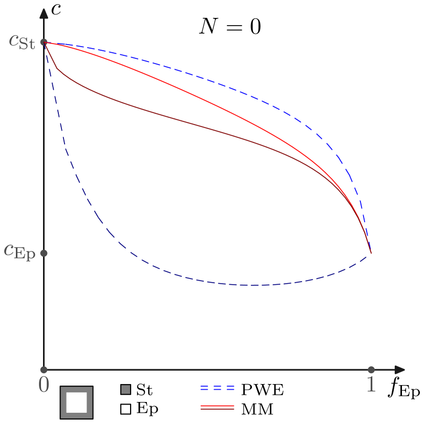
a)

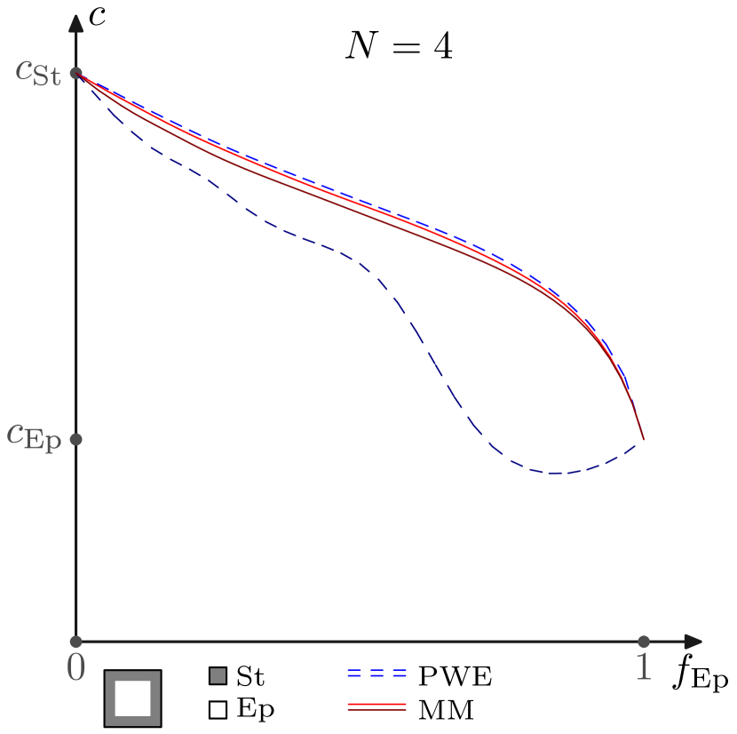
b)

Figure 1: PWE ($c_{NN}$, $\widetilde{c}_{NN}$) and MM ($c_{N}$, $\widetilde{c}_{N}$) bounds for Steel/Epoxy lattice of nested squares: a) $N=0$, b) $N=4$.

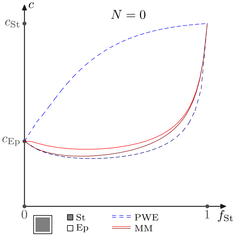
a)

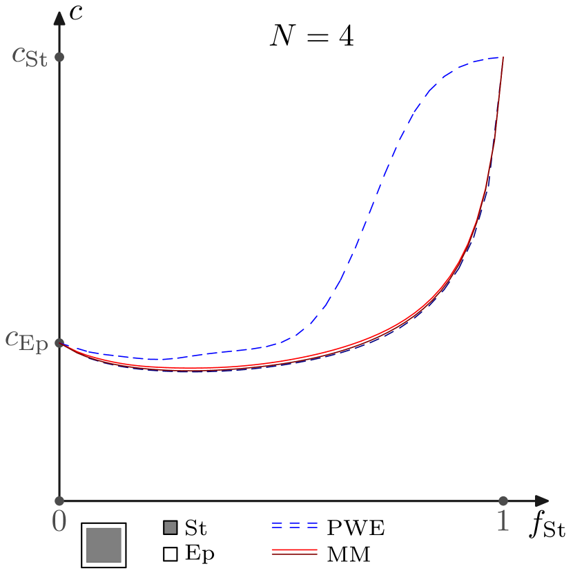
b)

Figure 2: PWE ($c_{NN}$, $\widetilde{c}_{NN}$) and MM ($c_{N}$, $\widetilde{c}_{N}$) bounds for Epoxy/Steel lattices of nested squares: a) $N=0$, b) $N=4$.

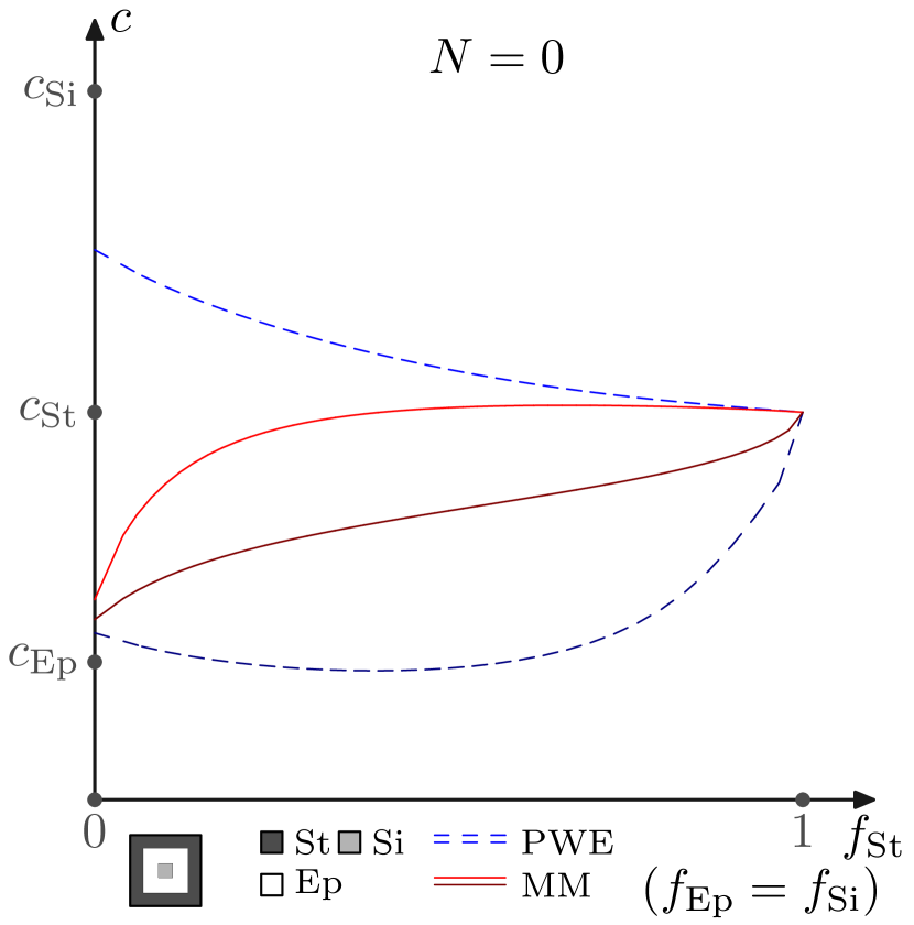
a)

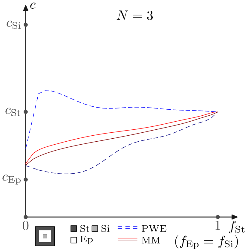
b)

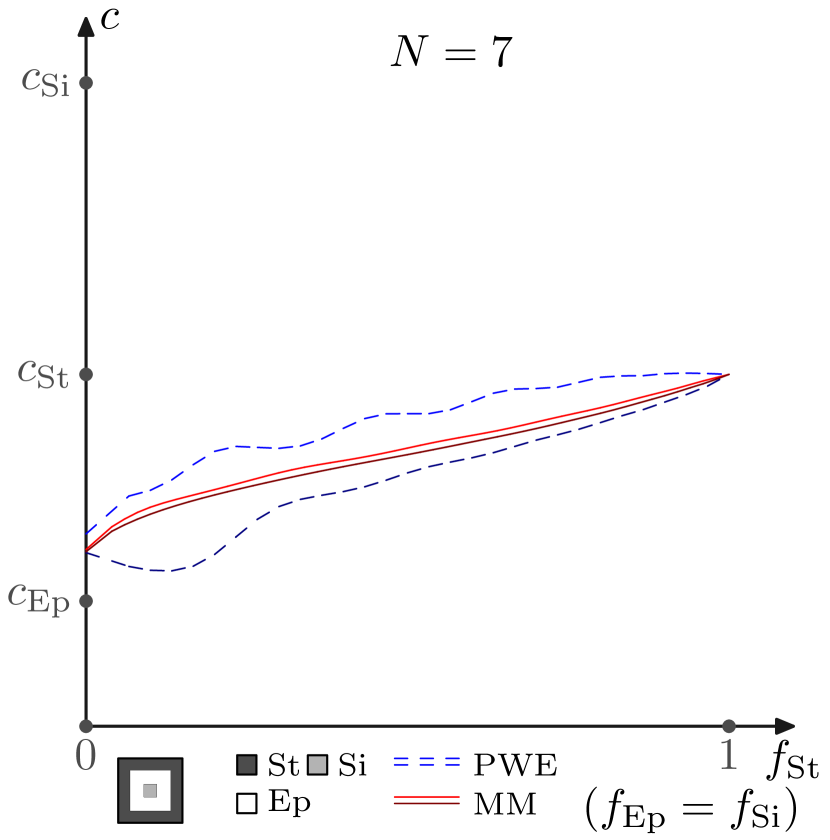
c)

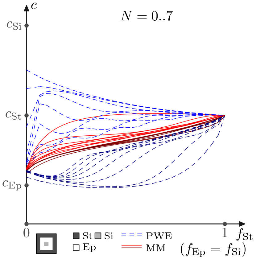
d)

Figure 3: PWE ($c_{NN}$, $\widetilde{c}_{NN}$) and MM ($c_{N}$, $\widetilde{c}_{N}$) bounds for Steel/Epoxy/Silicon lattice of nested squares: a) $N=0$, b) $N=3$, c) $N=7$, d) $N=0,...,7$.

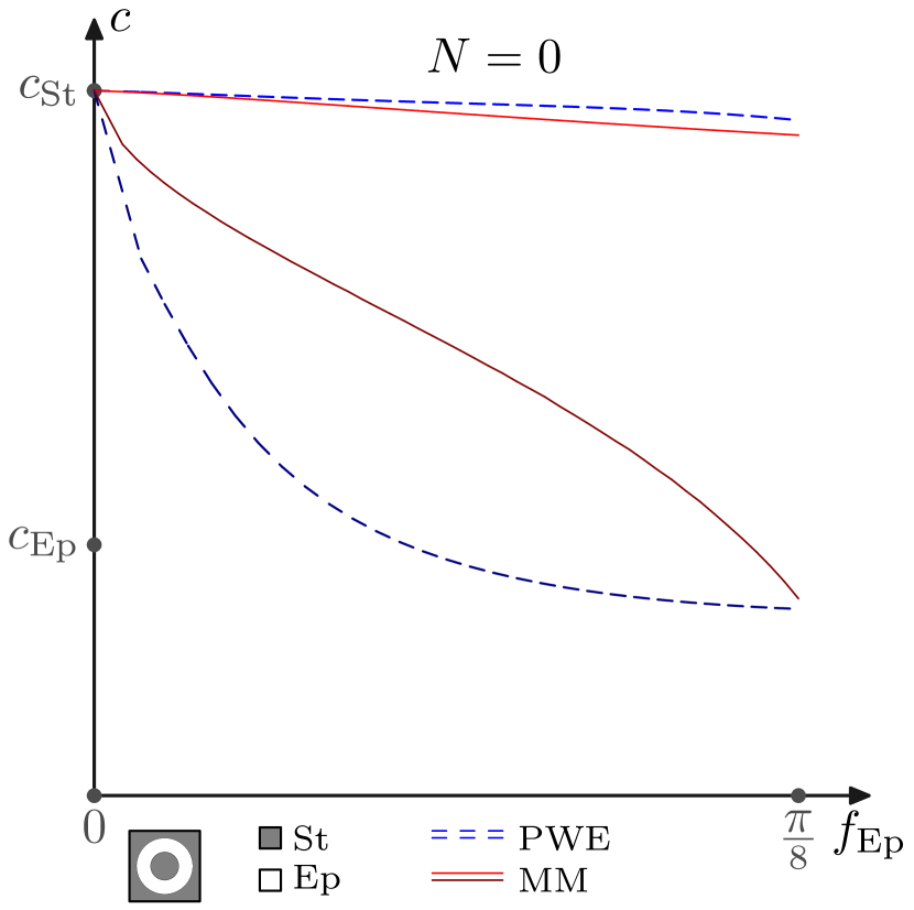
a)

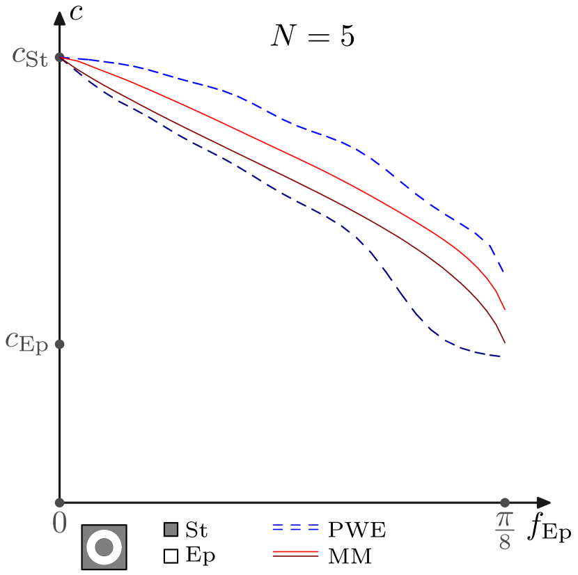
b)

Figure 4: PWE ($c_{NN}$, $\widetilde{c}_{NN}$) and MM ($c_{N}$, $\widetilde{c}_{N}$) bounds for Steel/Epoxy/Steel lattice of nested circles: a) $N=0$, b) $N=5$.

5 Proof of the main results

Lemma 1

Consider the eigenvalue problem

$${\bf A}{\bf u}=\lambda{\bf B}{\bf u}\ \ {\rm with}\ \ {\bf A}={\bf A}_{0}+k{\bf A}_{1}+k^{2}{\bf A}_{2},$$ (25)

where ${\bf A}$, ${\bf B}$ ($\mathop{\mathrm{det}}\nolimits{\bf B}\neq 0$) are self-adjoint matrices and $k$ is a small real parameter. Suppose that $\lambda=0$ for $k=0$ is a simple eigenvalue of ${\bf A}$ with normalized eigenvector ${\bf u}_{0}$ (${\bf u}_{0}\cdot{\bf u}_{0}=1$). Then

$$\lambda(k)=k\lambda_{1}+k^{2}\lambda_{2}+O(k^{3}),\ \ {\bf u}(k)={\bf u}_{0}+k{\bf u}_{1}+{\bf O}(k^{2}),$$ (26)

$$\lambda_{1}=\frac{{\bf A}_{1}{\bf u}_{0}\cdot{\bf u}_{0}}{{\bf B}{\bf u}_{0}\cdot{\bf u}_{0}},\ \ {\bf u}_{1}={\bf A}_{0}^{-1}(\lambda_{1}{\bf B}-{\bf A}_{1}){\bf u}_{0},\ \ \lambda_{2}=\frac{{\bf A}_{2}{\bf u}_{0}\cdot{\bf u}_{0}-{\bf A}_{0}{\bf u}_{1}\cdot{\bf u}_{1}}{{\bf B}{\bf u}_{0}\cdot{\bf u}_{0}}.$$ (27)

Proof. Substituting expansions (27) into (25) and equating the terms with the same power of $k$ we obtain

$${\bf A}_{0}{\bf u}_{1}+{\bf A}_{1}{\bf u}_{0}=\lambda_{1}{\bf B}{\bf u}_{0},$$ (28)

$${\bf A}_{0}{\bf u}_{2}+{\bf A}_{1}{\bf u}_{1}+{\bf A}_{2}{\bf u}_{0}=\lambda_{2}{\bf B}{\bf u}_{0}+\lambda_{1}{\bf B}{\bf u}_{1}.$$ (29)

Scalar multiplying both sides in (28), (29) by ${\bf u}_{0}$, using ${\bf A}_{0}{\bf u}_{0}={\bf 0}$ and self-adjointness of ${\bf A}_{i}$, ${\bf B}$ we obtain (27).   

5.1 Proof of Theorem 3.1

According to (4) and (8), the effective shear coefficient $\mu_{\rm eff}$ given by (8)₂ can be defined as

$$\mu_{\rm eff}=\lim_{k\to 0}\frac{\omega_{1}^{2}}{k^{2}},$$ (30)

where $\omega_{1}$ is a minimal eigenvalue of the eigenproblem (1) with $\rho=1$, i.e. of

$${\mathcal{C}}({\bf k})u=\omega^{2}({\bf k})u.$$ (31)

Introduce the subspace ${\mathcal{L}}_{NN}$ of $L^{2}([0,1]^{2})$,

$${\mathcal{L}}_{NN}={\mathcal{L}}(\{e^{2\pi i(g_{1}x_{1}+g_{2}x_{2})}:\ \ |g_{1}|,|g_{2}|\leqslant N\}),$$ (32)

where ${\mathcal{L}}(\cdot)$ means the linear span of the set. Denote the corresponding projector ${\mathcal{P}}_{NN}:L^{2}([0,1]^{2})\to{\mathcal{L}}_{NN}$. Consider the equation

$${\mathcal{C}}_{NN}({\bf k})u=\omega^{2}_{NN}({\bf k})u$$ (33)

with

$${\mathcal{C}}_{NN}({\bf k}):{\mathcal{L}}_{NN}\to{\mathcal{L}}_{NN},\ \ \ {\mathcal{C}}_{NN}({\bf k})\equiv{\mathcal{P}}_{NN}{\mathcal{C}}({\bf k}).$$ (34)

The operator ${\mathcal{C}}_{NN}$ can be represented as a finite matrix

$${\mathcal{C}}_{NN}({\bf k})=(\widehat{{\mu}}({\bf g}-{\bf g}^{\prime})(2\pi{\bf g}+{\bf k})\cdot(2\pi{\bf g}^{\prime}+{\bf k}))_{|g_{i}^{\prime}|,|g_{i}|\leqslant N},$$ (35)

where $\widehat{{\mu}}$ are Fourier coefficients for ${\mu}$ (see (10)). Note that the minimal eigenvalue $\omega_{1,NN}({\bf k})$ of ${\mathcal{C}}_{NN}({\bf k})$ is greater than the minimal eigenvalue $\omega_{1}({\bf k})$ of ${\mathcal{C}}({\bf k})$, since

$$\omega_{1}({\bf k})=\inf_{u\in{\mathcal{H}}}\frac{({\mathcal{C}}({\bf k})u,u)}{(u,u)}\leqslant\inf_{u\in{\mathcal{L}}_{NN}}\frac{({\mathcal{C}}({\bf k})u,u)}{(u,u)}=\inf_{u\in{\mathcal{L}}_{NN}}\frac{({\mathcal{C}}_{NN}({\bf k})u,u)}{(u,u)}=\omega_{1,NN}({\bf k}),$$ (36)

where ${\mathcal{H}}$ is a Sobolev space. Also $\omega_{1,NN}\searrow\omega_{1}$ for $N\to\infty$, since ${\mathcal{L}}_{N^{\prime}N^{\prime}}\subset{\mathcal{L}}_{NN}$ for $N^{\prime}\leqslant N$ and $\cup_{N}{\mathcal{L}}_{NN}$ is dense in ${\mathcal{H}}$. Denote the limit

$$b_{NN}(\boldsymbol{\kappa})=\lim_{k\to 0}\frac{\omega^{2}_{1,NN}({\bf k})}{k^{2}}\ \ \ ({\bf k}=k\boldsymbol{\kappa},\ \ \|\boldsymbol{\kappa}\|=1).$$ (37)

By (36), $b_{NN}$ is greater than $\mu_{\rm eff}$ and $b_{NN}\searrow\mu_{\rm eff}$ for $N\to\infty$. Taking ${\bf k}=k{\bf e}_{1}$ ($\boldsymbol{\kappa}={\bf e}_{1}$) in (35) leads to

$${\mathcal{C}}_{NN}={\mathcal{C}}_{NN,0}+k{\mathcal{C}}_{NN,1}+k^{2}{\mathcal{C}}_{NN,2}\ \ {\rm where}\\ {\mathcal{C}}_{NN,1}=2\pi((g_{1}+g^{\prime}_{1})\widehat{{\mu}}({\bf g}-{\bf g}^{\prime}))_{|g_{i}|\leqslant N},\ \ {\mathcal{C}}_{NN,2}=(\widehat{{\mu}}({\bf g}-{\bf g}^{\prime}))_{|g_{i}|\leqslant N}$$ (38)

and ${\mathcal{C}}_{NN,0}$ is given by (11). Applying Lemma 1 to ${\bf A}={\mathcal{C}}_{NN}$, ${\bf B}={\bf I}$ with ${\bf u}_{0}=(\delta_{{\bf g}{\bf 0}})_{|g_{i}|\leqslant N}$ and $\lambda=\omega_{1,NN}^{2}=\lambda_{1}k+b_{NN}k^{2}+...$ yields $\lambda_{1}=0$ and $b_{NN}=\mu_{NN}$, where $\mu_{NN}$ is given by (12)₁. Since $b_{NN}\searrow\mu_{\rm eff}$ (see above), we conclude that $\mu_{NN}\searrow\mu_{\rm eff}$. Applying the same steps to $\mu^{-1}$ and using (9), (12)₂ we obtain ${\widetilde{\mu}}_{NN}\nearrow\mu_{\rm eff}$. Thus (13) is proved.   

5.2 Proof of Theorem 3.2

As in the previous section, we proceed from equation (33). Introduce the subspace ${\mathcal{L}}_{N}$ of ${\mathcal{H}}_{\bf k}=e^{i{\bf k}\cdot{\bf x}}{\mathcal{H}}$,

$${\mathcal{L}}_{N}={\mathcal{L}}(\{e^{i\bf{k}\cdot{\bf x}}e^{2\pi i(g_{1}x_{1}+g_{2}x_{2})}:\ \ g_{1}\in{\mathbb{Z}},\ |g_{2}|\leqslant N\}),$$ (39)

and the corresponding projector ${\mathcal{P}}_{N}:{\mathcal{H}}_{\bf k}\to{\mathcal{L}}_{N}$. Consider the equation

$${\mathcal{C}}_{N}({\bf k})u=\omega^{2}_{N}({\bf k})u$$ (40)

with

$${\mathcal{C}}_{N}({\bf k}):{\mathcal{L}}_{N}\to{\mathcal{L}}_{N},\ \ \ {\mathcal{C}}_{N}({\bf k})\equiv{\mathcal{P}}_{N}{\mathcal{C}}({\bf k}).$$ (41)

Suppose that ${\bf k}=\begin{pmatrix}k_{1}&0\end{pmatrix}^{\top}$, i.e. $k_{2}=0$. Let $\omega_{1,N}$ be the minimal eigenvalue in (40), and denote the limit

$$b_{N}=\lim_{k_{1}\to 0}\frac{\omega^{2}_{1,N}(k_{1}{\bf e}_{1})}{k^{2}_{1}}.$$ (42)

Repeating arguments from (36) to the end of §5.1 and using the fact that $e^{i{\bf k}\cdot{\bf x}}{\mathcal{L}}_{NN}\subset{\mathcal{L}}_{N}$ (see (32), (39)) we obtain

$$b_{N}\searrow\mu_{\rm eff},\ \ (\mu_{NN}=)b_{NN}\geqslant b_{N}.$$ (43)

In order to complete the proof, we need to show that $b_{N}=\mu_{N}$. The operator ${\mathcal{C}}_{N}$ can be represented as a 1D vector differential operator

$${\mathcal{C}}_{N}=-\partial_{1}\widehat{\boldsymbol{\mu}}_{N}\partial_{1}+\boldsymbol{\partial}_{N}\widehat{\boldsymbol{\mu}}_{N}\boldsymbol{\partial}_{N},$$ (44)

where the notations (15) are used. Equation (40) can be rewritten in the form

$$\partial_{1}\boldsymbol{\eta}=\widetilde{\bf Q}_{N}\boldsymbol{\eta}\ \ {\rm with}\quad\left\{\begin{aligned} \boldsymbol{\eta}=\begin{pmatrix}{\bf u}_{N}&\widehat{\boldsymbol{\mu}}_{N}\partial_{1}{\bf u}_{N}\end{pmatrix}^{\top},\ \ {\bf u}_{N}(x_{1})&=\big{(}\widehat{u}_{n}(x_{1})\big{)}_{n=-N}^{N},\\ \quad\widetilde{\bf Q}_{N}=\begin{pmatrix}{\bf 0}&\widehat{\boldsymbol{\mu}}_{N}^{-1}\\ \boldsymbol{\partial}_{N}\widehat{\boldsymbol{\mu}}_{N}\boldsymbol{\partial}_{N}-\omega_{N}^{2}{\bf I}&{\bf 0}\end{pmatrix}.\end{aligned}\right.$$ (45)

The solution of (45) has the following form

$$\boldsymbol{\eta}(x_{1})=\widetilde{\bf M}_{N}[x_{1},0]\boldsymbol{\eta}(0)\ \ {\rm with}\ \ \widetilde{\bf M}_{N}[\beta,\alpha]=\widehat{\int_{\alpha}^{\beta}}({\bf I}+\widetilde{\bf Q}_{N}dx_{1}).$$ (46)

Taking $x_{1}=1$ in (46) and noting that $\boldsymbol{\eta}=e^{ik_{1}x_{1}}\boldsymbol{\xi}$ with periodic $\boldsymbol{\xi}$ (see (39)) we obtain

$$e^{ik_{1}}\boldsymbol{\xi}(0)=\widetilde{\bf M}_{N}[1,0]\boldsymbol{\xi}(0).$$ (47)

In order to find $b_{N}$ (42) we need the asymptotics of each term in (47). Using (42), we expand $\widetilde{\bf Q}_{N}$ (45) as

$$\widetilde{\bf Q}_{N}={\bf Q}_{N}+k_{1}^{2}b_{N}{\bf Q}_{2,N}+...\ \ {\rm with}\ \ {\bf Q}_{2,N}=\begin{pmatrix}{\bf 0}&{\bf 0}\\ -{\bf I}&{\bf 0}\end{pmatrix}$$ (48)

and substitute it into (46)₂ to obtain

$$\widetilde{\bf M}_{N}[1,0]={\bf M}_{N}+k_{1}^{2}b_{N}{\bf M}_{2,N}+...\ \ {\rm with}\\ {\bf M}_{2,N}=\int_{0}^{1}{\bf M}_{N}[1,x]{\bf Q}_{2,N}(x){\bf M}_{N}[x,0]dx,\ \ {\bf M}_{N}[\beta,\alpha]=\widehat{\int_{\alpha}^{\beta}}({\bf I}+{\bf Q}_{N}dx_{1}),$$ (49)

where ${\bf Q}_{N}$ and ${\bf M}_{N}={\bf M}_{N}[1,0]$ are given in (16). Note that

$${\bf Q}_{N}{\bf w}_{1}={\bf 0},\ \ {\bf w}_{2}^{*}{\bf Q}_{N}={\bf 0}$$ (50)

for ${\bf w}_{i}$ defined in (18), since ${\bf e}_{(N)}^{*}\boldsymbol{\partial}_{N}=\boldsymbol{\partial}_{N}{\bf e}_{(N)}={\bf 0}$. Combining (50) with (16)₂ yields

$${\bf M}_{N}[\beta,\alpha]{\bf w}_{1}={\bf w}_{1},\ \ {\bf w}_{2}^{*}{\bf M}_{N}[\beta,\alpha]={\bf w}_{2}^{*},\ \ \forall\,\alpha,\beta.$$ (51)

Hence, by (49) and (51), the vector $\boldsymbol{\xi}(0)$ in (47) satisfies

$$\boldsymbol{\xi}(0)={\bf w}_{1}+k_{1}\boldsymbol{\xi}_{1}+k_{1}^{2}\boldsymbol{\xi}_{2}+...$$ (52)

with unknown $\boldsymbol{\xi}_{1}$, $\boldsymbol{\xi}_{2},\ldots$. Substituting (52), (49) with $e^{ik_{1}}=1+ik_{1}-\frac{1}{2}{k_{1}^{2}}+...$ into (47) and equating terms with the same power of $k_{1}$ yields

$$\boldsymbol{\xi}_{1}=i({\bf M}_{N}-{\bf I})^{-1}{\bf w}_{1},$$ (53)

$${\bf M}_{N}\boldsymbol{\xi}_{2}+b_{N}{\bf M}_{2,N}{\bf w}_{1}=\boldsymbol{\xi}_{2}+i\boldsymbol{\xi}_{1}-\frac{1}{2}{\bf w}_{1}.$$ (54)

Multiplying (54) by the vector ${\bf w}_{2}^{*}$ and using (51) along with ${\bf w}_{2}^{*}{\bf w}_{1}=0$, we obtain

$$b_{N}={\bf w}_{2}^{*}({\bf M}_{N}-{\bf I})^{-1}{\bf w}_{1},$$ (55)

which coincides with $\mu_{N}$ in (17). Thus (43) yields (19), (20) for the upper bound $\mu_{N}$. The proof for the lower bound $\widetilde{\mu}_{N}$ is similar.   

5.3 Proof of Theorem 3.3

Taking (55) with $b_{N}=\mu_{N}$, applying the chain rule, and using (51), we obtain

$$\mu_{N}={\bf w}_{2}^{*}({\bf M}_{N}-{\bf I})^{-1}{\bf w}_{1}={\bf w}_{2}^{*}({\bf M}_{N}[\tfrac{1}{2},0]-{\bf M}_{N}[\tfrac{1}{2},1])^{-1}{\bf w}_{1}.$$ (56)

The definition (49) of ${\bf M}_{N}[\beta,\alpha]$ and the ${\bf 1}$-periodicity of $\mu$ with symmetry $\mu(x_{1},x_{2})=\mu(-x_{1},x_{2})$ give us

$${\bf M}_{N}[\tfrac{1}{2},0]=\widehat{\int_{0}^{\frac{1}{2}}}({\bf I}+{\bf Q}_{N}dx_{1}),\ \ {\bf M}_{N}[\tfrac{1}{2},1]=\widehat{\int_{0}^{\frac{1}{2}}}({\bf I}-{\bf Q}_{N}dx_{1}).$$ (57)

Due to (57) we get

$${\bf M}_{N}[\tfrac{1}{2},0]=\begin{pmatrix}{\bf a}_{1}&{\bf a}_{2}\\ {\bf a}_{3}&{\bf a}_{4}\end{pmatrix},\ \ {\bf M}_{N}[\tfrac{1}{2},1]=\begin{pmatrix}{\bf a}_{1}&-{\bf a}_{2}\\ -{\bf a}_{3}&{\bf a}_{4}\end{pmatrix},$$ (58)

since blocks of ${\bf Q}_{N}$ on the diagonal are zero matrices, see (16). Equalities (56), (58) and ${\bf M}_{N,\frac{1}{2}}={\bf M}_{N}[\tfrac{1}{2},0]$ lead to (22)₁. The proof of (22)₂ is similar.   

6 Conclusion

The PWE and MM bounds of the effective speed $c$ have been presented. It was shown that the MM bounds $c_{N}$, $\widetilde{c}_{N}$ are more accurate than the PWE bounds $c_{NN}$, $\widetilde{c}_{NN}$. In fact even for not so large $N$ it is often sufficient to use only one MM bound $c_{N}$ or $\widetilde{c}_{N}$ to obtain a good enough approximation of $c$.

Moreover, numerical implementation of the MM scheme requires less computation time per step than the PWE method, since the former needs to calculate an exponent of $(4N+2)\times(4N+2)$ matrix and to solve a system of $(4N+2)$ linear equations whereas the latter needs to solve a system of $(2N+1)^{2}$ linear equations.

The results of the paper apply to other types of scalar waves described by the governing equations similar to (1), such as acoustic waves in fluids, and electromagnetic waves.

A Appendix

A.1 Example of a closed form $c(\boldsymbol{\kappa})$

Suppose that $\mu=\mu_{1}(x_{1})\mu_{2}(x_{2})$. Then $c(\boldsymbol{\kappa})$ admits a closed-form representation

$$c^{2}(\boldsymbol{\kappa})=\frac{1}{\langle\rho\rangle}\boldsymbol{\kappa}^{\top}\begin{pmatrix}\langle\mu_{2}\rangle_{2}\langle\mu_{1}^{-1}\rangle_{1}^{-1}&0\\ 0&\langle\mu_{1}\rangle_{1}\langle\mu_{2}^{-1}\rangle_{2}^{-1}\end{pmatrix}\boldsymbol{\kappa},$$ (A.1)

where $\langle\cdot\rangle_{i}=\int_{0}^{1}\cdot dx_{i}$. The proof of (A.1) is based on the fact that the equation ${\mathcal{C}}_{0}h={\mathcal{C}}_{1}u_{1}$ (see (5)) has closed-form solution $h={\mathcal{C}}_{0}^{-1}{\mathcal{C}}_{1}u_{1}$. Let $\boldsymbol{\kappa}={\bf e}_{1}$, then

$${\mathcal{C}}_{0}h={\mathcal{C}}_{1}u_{1}\ \Rightarrow\ -\mu_{2}\partial_{1}(\mu_{1}\partial_{1}h)-\mu_{1}\partial_{2}(\mu_{2}\partial_{2}h)=-i\mu_{2}\partial_{1}\mu_{1}.$$ (A.2)

Assume the solution of (A.2) in the form $h=h(x_{1})$, then

$$\partial_{1}(\mu_{1}\partial_{1}h)=i\partial_{1}\mu_{1}\ \Rightarrow\ \mu_{1}\partial_{1}h=i\mu_{1}+\alpha_{1}\ \Rightarrow\ h=\alpha_{2}+ix_{1}+\alpha_{1}\int_{0}^{x_{1}}\mu_{1}^{-1}dx_{1},$$ (A.3)

$$h(1)=h(0)\ \Rightarrow\ h=\alpha_{2}+ix_{1}-i\langle\mu_{1}^{-1}\rangle^{-1}\int_{0}^{x_{1}}\mu_{1}^{-1}dx_{1}\ \ (\alpha_{2}=\mathop{\mathrm{const}}\nolimits).$$ (A.4)

Substituting $h={\mathcal{C}}_{0}^{-1}{\mathcal{C}}_{1}u_{1}$ from (A.4) into (6) gives the upper left element of the matrix in (A.1). Other elements are obtained similarly. If $\mu$ depends on $x_{1}$ only, then (A.1) reduces to the well-known result $\langle\rho\rangle c^{2}=\langle\mu^{-1}\rangle^{-1}{\kappa_{1}}^{2}+\langle\mu\rangle\kappa_{2}^{2}$.

A.2 Options for calculating the multiplicative integral

By definition, the multiplicative integral ${\bf M}[\beta,\alpha]=\widehat{\int}_{\alpha}^{\beta}({\bf I}+{\bf Q}dx)$ is

$${\bf M}=\lim_{k\to\infty}\prod_{j=[\alpha k]}^{[\beta k]}({\bf I}+(1/k){\bf Q}(j/k)),$$ (A.5)

where $[\cdot]$ denotes integer part. This formula is straightforward for numerical implementation. It was employed for calculating (21) to obtain the MM curves for circular inclusions, see Fig.4.

Another method is to use the Peano series

$${\bf M}={\bf I}+\int_{\alpha}^{\beta}{\bf Q}(y_{1})dy_{1}+\int_{\alpha}^{\beta}\int_{\alpha}^{y_{1}}{\bf Q}(y_{1}){\bf Q}(y_{2})dy_{1}dy_{2}+....$$ (A.6)

It converges faster than (A.5) (at the same rate as the series for exponent of ${\bf Q}$) but its implementation is more laborious.

If ${\bf Q}(x)$ is a piecewise constant function on $[\alpha,\beta]$, i.e.

$${\bf Q}(x)=\mathop{\mathrm{const}}\nolimits_{i}\ {\rm for}\ x\in\Delta_{i}\ {\rm where}\\ [\alpha,\beta]=\cup_{i=1}^{n}\Delta_{i},\ \ \Delta_{i}=[x_{i-1},x_{i}),\ \ \alpha=x_{0}<x_{1}<...<x_{n}=\beta,$$ (A.7)

then

$${\bf M}=\exp(|\Delta_{n}|{\bf Q}(x_{n-1}))...\exp(|\Delta_{1}|{\bf Q}(x_{0})).$$ (A.8)

This formula was used for calculating (21) to obtain the MM curves in Figs. 1-3.

Note in conclusion that the principal formula (17) involves the resolvent $({\bf M}_{N}-{\bf I})^{-1}$, which can be calculated directly (i.e. without evaluating ${\bf M}_{N}$) by numerical integration of the corresponding Riccati equation. In fact using the resolvent has some numerical advantage, because the increase of its elements with growing $N$ is slower than the increase of elements of ${\bf M}_{N}$.

References

• (1) A. A. Krokhin, J. Arriaga, L. N. Gumen, ”Speed of sound in periodic elastic composites”, Phys. Rev. Lett. 91, 264302 (2003)
• (2) A. A. Kutsenko, A. L. Shuvalov, A. N. Norris, O. Poncelet, ”Effective shear speed in two-dimensional phononic crystals”, Phys. Rev. B, 84, 064305 (2011).
• (3) A. A. Kutsenko, A. L. Shuvalov, A. N. Norris, ”Evaluation of the effective speed of sound in phononic crystals by the monodromy matrix method”, J. Acoust. Soc. Am., 130, 3553–3557 (2011).
• (4) J. Nevard, J. B. Keller, ”Reciprocal relations for effective conductivities of anisotropic media”, J. Math. Phys., 26, 2761–2765 (1985).
• (5) V. V. Jikov, S. M. Kozlov, O. A. Oleinik, Homogenization of Differential Operators and Integral Functionals, Springer-Verlag, New York (1994).
• (6) M. Reed, B. Simon, Methods of Modern Mathematical Physics. IV. Analysis of Operators, Academic Press, New York - London (1978).
• (7) M. C. Pease, III, Methods of Matrix Algebra, Academic Press, New York (1965).