The Beta-MANOVA Ensemble with General Covariance

Abstract

We find the joint generalized singular value distribution and largest generalized singular value distributions of the $\beta$-MANOVA ensemble with positive diagonal covariance, which is general. This has been done for the continuous $\beta>0$ case for identity covariance (in eigenvalue form), and by setting the covariance to $I$ in our model we get another version. For the diagonal covariance case, it has only been done for $\beta=1,2,4$ cases (real, complex, and quaternion matrix entries). This is in a way the first second-order $\beta$-ensemble, since the sampler for the generalized singular values of the $\beta$-MANOVA with diagonal covariance calls the sampler for the eigenvalues of the $\beta$-Wishart with diagonal covariance of Forrester and Dubbs-Edelman-Koev-Venkataramana. We use a conjecture of MacDonald proven by Baker and Forrester concerning an integral of a hypergeometric function and a theorem of Kaneko concerning an integral of Jack polynomials to derive our generalized singular value distributions. In addition we use many identities from Forrester’s Log-Gases and Random Matrices. We supply numerical evidence that our theorems are correct.

Mathematics Subject Classification 2000: 22E46, 53C35, 57S20

1 Introduction

The first $\beta$-ensembles were introduced by Dumitriu and Edelman [1], the $\beta$-Hermite ensemble and the $\beta$-Laguerre ensemble. A $\beta$- ensemble is defined to be a real random matrix with a nonrandom continuous tuning parameter $\beta>0$ such that when $\beta=1,2,4$, the $\beta$- ensemble has the same joint eigenvalue distribution as the real, complex, or quaternionic -ensemble. For $\beta$ not equal to $1,2,4$ its eigenvalue distribution interpolates naturally among the $\beta=1,2,4$ cases. A $\beta$-circular ensemble and four $\beta$-Jacobi ensembles shortly followed [2], [3], [4], [5]. The extreme eigenvalues of the $\beta$-Jacobi ensembles were characterized by Dumitriu and Koev in [6]. More recently, Forrester [7] and Dubbs-Edelman-Koev-Venkataramana [8] separately introduced a $\beta$-Wishart ensemble with diagonal covariance, which generalizes the $\beta$-Laguerre ensemble by adding the covariance term.

This paper introduces the $\beta$-MANOVA ensemble with diagonal covariance, which generalizes the $\beta$-Jacobi ensembles by adding the covariance term. When $\beta=1$ this amounts to finding the distribution of the cosine generalized singular values of the pair $(Y,X\Omega)$, where $X$ is $m\times n$ Gaussian, $Y$ is $p\times n$ Gaussian, and $\Omega$ is $n\times n$ diagonal pds. Note that forcing $\Omega$ to be diagonal does not lose any generality; using orthogonal transformations, were $\Omega$ not diagonal we could replace it with its diagonal matrix of eigenvalues and preserve the model. Our $\beta$-MANOVA ensemble also generalizes the real, complex, and quaternionic MANOVA ensembles (the last of which has never been studied). [9], [10], and [11] independently solved the $\beta=1$ identity-covariance case, [12] solved our problem in the $\beta=1$, general-covariance case, and [13] solved our problem in the $\beta=2$, general-covariance case. We find the joint eigenvalue distribution of the $\beta$-MANOVA ensemble, and generalize Dumitriu and Koev’s results in [6] by finding the distribution of the largest generalized singular value of the $\beta$-MANOVA ensemble. We also set the covariance to the identity to add a fourth $\beta$-Jacobi ensemble to the literature in Theorem 3.1. Our $\beta$-MANOVA ensemble is unique in that it is not built on a recursive procedure, rather it is sampled by calling the sampler for the $\beta$-Wishart ensemble.

Generalizations of our results exist in the $\beta=1,2$ cases by adding a mean matrix to one of the Wishart-distributed parameters. The $\beta=1$ case is from [12, p. 1279] and the $\beta=2$ case is from [13, p. 490].

The sampler for the $\beta$-Wishart ensemble of Forrester [7] and Dubbs-Edelman-Koev-Venkataramana [8] is the following algorithm:

Beta-Wishart (Recursive) Model Pseudocode Function $\Sigma$ := BetaWishart$(m,n,\beta,D)$ if $n=1$ then      $\Sigma$ := $\chi_{m\beta}D_{1,1}^{1/2}$ else      $Z_{1:n-1,1:n-1}$ := BetaWishart$(m,n-1,\beta,D_{1:n-1,1:n-1})$      $Z_{n,1:n-1}$ := $[0,\ldots,0]$      $Z_{1:n-1,n}$ := $[\chi_{\beta}D_{n,n}^{1/2};\ldots;\chi_{\beta}D_{n,n}^{1/2}]$      $Z_{n,n}$ := $\chi_{(m-n+1)\beta}D_{n,n}^{1/2}$      $\Sigma$ := diag(svd($Z$)) end if

The elements of $\Sigma$ are distributed according to the following theorem of [7] and [8]:

Proposition 1.1.

The distribution of the singular values ${\rm diag}(\Sigma)=(\sigma_{1},\ldots,\sigma_{n})$, $\sigma_{1}>\sigma_{2}>\cdots>\sigma_{n}$, generated by the above algorithm is equal to:

$$\frac{2^{n}\det(D)^{-m\beta/2}}{\mathcal{K}_{m,n}^{(\beta)}}\prod_{i=1}^{n}\sigma_{i}^{(m-n+1)\beta-1}\Delta^{2}(\sigma)^{\beta}{{{}_{0}F_{0}}}^{\!\!(\beta)}\left(-\frac{1}{2}\Sigma^{2},D^{-1}\right)d\sigma,$$

where ${{{}_{0}F_{0}}}^{\!\!(\beta)}$ and $\mathcal{K}^{(\beta)}_{m,n}$ are defined in the upcoming section, Preliminaries.

To get the generalized singular values of the $\beta$-MANOVA ensemble with general covariance, in diagonal $C$, we use the following algorithm which calls ${\rm BetaWishart}(m,n,\beta,D)$. Let $\Omega$ be an $n\times n$ diagonal matrix.

Beta-MANOVA Model Pseudocode Function $C$ := BetaMANOVA$(m,n,p,\beta,\Omega)$ $\Lambda:={\rm BetaWishart}(m,n,\beta,\Omega^{2})$ $M:={\rm BetaWishart}(p,n,\beta,\Lambda^{-1})^{-1}$ $C:=(M+I)^{-\frac{1}{2}}$

Our main theorem is the joint distribution of the elements of $C$,

Theorem 1.2.

The distribution of the generalized singular values ${\rm diag}(C)=(c_{1},\ldots,c_{n})$, $c_{1}>c_{2}>\cdots>c_{n}$, generated by the above algorithm for $m,p\geq n$ is equal to:

$$\frac{2^{n}\mathcal{K}_{m+p,n}^{(\beta)}}{\mathcal{K}_{m,n}^{(\beta)}\mathcal{K}_{p,n}^{(\beta)}}\det(\Omega)^{p\beta}\prod_{i=1}^{n}c_{i}^{(p-n+1)\beta-1}\prod_{i=1}^{n}(1-c_{i}^{2})^{-\frac{p+n-1}{2}\beta-1}\prod_{i<j}|c_{i}^{2}-c_{j}^{2}|^{\beta}\\ \times{{}_{1}F_{0}}^{\!\!(\beta)}\left(\frac{m+p}{2}\cdot\beta;;C^{2}(C^{2}-I)^{-1},\Omega^{2}\right)dc.$$

where ${{{}_{1}F_{0}}}^{\!\!(\beta)}$ and $\mathcal{K}^{(\beta)}_{m,n}$ are defined in the upcoming section, Preliminaries.

We also find the distributions of the largest generalized singular value in certain cases:

Theorem 1.3.

If $t=(m-n+1)\beta/2-1\in\mathbb{Z}_{\geq 0}$,

$$P(c_{1}<x)=\det(x^{2}\Omega^{2}((1-x^{2})I+x^{2}\Omega^{2})^{-1})^{\frac{p\beta}{2}}\\ \times\sum_{k=0}^{nt}\sum_{\kappa\vdash k,\kappa_{1}\leq t}\frac{1}{k!}(p\beta/2)_{\kappa}^{(\beta)}C_{\kappa}^{(\beta)}\left((1-x^{2})((1-x^{2})I+x^{2}\Omega^{2})^{-1}\right),$$ (1)

where the Jack function $C_{\kappa}^{(\beta)}$ and Pochhammer symbol $(\cdot)_{\kappa}^{(\beta)}$ are defined in the upcoming section, Preliminaries.

These expressions can be computed by Edelman and Koev’s software, mhg, [14].

It is actually intuitive that ${\rm BetaMANOVA}(m,n,p,\beta,\Omega)$ should generalize the real, complex, and quaternionic MANOVA ensembles with diagonal covariance using the “method of ghosts.” The method of ghosts was first used implicitly to derive $\beta$-ensembles for the Laguerre and Hermite cases in [1], was stated precisely by Edelman in [15], and was expanded on in [8]. To use the method of ghosts, assume a given ensemble is full of $\beta$-dimensional Gaussians, which generalize real, complex, and quaternionic Gaussians and have some of the same properties: they can be left invariant or made into a $\chi_{\beta}$’s under rotation by a real orthogonal or “ghost orthogonal” matrix. Then apply enough orthogonal transformations and/or ghost orthogonal transformations to the ghost matrix to make it all real.

In the $\beta$-MANOVA case, let $X$ be $m\times n$ real, complex, quaternion, or ghost normal, $Y$ be $p\times n$ real complex, quaternion, or ghost normal, and let $\Omega$ be $n\times n$ diagonal real pds. Let $\Omega X^{*}X\Omega$ have eigendecomposition $U\Lambda U^{*}$, and $\Omega X^{*}X\Omega(Y^{*}Y)^{-1}$ have eigendecomposition $VMV^{*}$. We want to draw $M$ so we can draw $C={\rm gsvd}_{(\rm cosine)}(Y,X\Omega)=(M+I)^{-\frac{1}{2}}$. Let $\sim$ mean “having the same eigenvalues.”

$$\Omega X^{*}X\Omega(Y^{*}Y)^{-1}\sim\Lambda U^{*}(Y^{*}Y)^{-1}U\sim\Lambda((U^{*}Y^{*})(YU))^{-1}\sim\Lambda(Y^{*}Y)^{-1},$$

which we can draw the eigenvalues $M$ of using ${\rm BetaWishart}(p,n,\beta,\Lambda^{-1})^{-1}$. Since $\Lambda$ can be drawn using ${\rm BetaWishart}(m,n,\beta,\Omega^{2})$, this completes the algorithm for ${\rm BetaMANOVA}(m,n,p,\beta,\Omega)$ and proves Theorem 1.1 in the $\beta=1,2,4$ cases.

The following section contains preliminaries to the proofs of Theorems 1.1 and 1.2 in the general $\beta$ case. Most important are several propositions concerning Jack polynomials and Hypergeometric Functions. Proposition 2.1 was conjectured by Macdonald [16] and proved by Baker and Forrester [17], Proposition 2.3 is due to Kaneko, in a paper containing many results on Selberg-type integrals [18], and the other propositions are found in [19, pp. 593-596].

2 Preliminaries

Definition 2.1.

We define the generalized Gamma function to be

$$\Gamma_{n}^{(\beta)}(c)=\pi^{n(n-1)\beta/4}\prod_{i=1}^{n}\Gamma(c-(i-1)\beta/2)$$

for $\Re(c)>(n-1)\beta/2$.

Definition 2.2.

$$\mathcal{K}_{m,n}^{(\beta)}=\frac{2^{mn\beta/2}}{\pi^{n(n-1)\beta/2}}\cdot\frac{\Gamma_{n}^{(\beta)}(m\beta/2)\Gamma_{n}^{\beta}(n\beta/2)}{\Gamma(\beta/2)^{n}}.$$

Definition 2.3.

$$\Delta(\lambda)=\prod_{i<j}(\lambda_{i}-\lambda_{j}).$$

If $X$ is a diagonal matrix,

$$\Delta(X)=\prod_{i<j}|X_{i,i}-X_{j,j}|.$$

As in Dumitriu, Edelman, and Shuman, if $\kappa\vdash k$, $\kappa=(\kappa_{1},\kappa_{2},\ldots,\kappa_{n})$ is nonnegative, ordered non-increasingly, and it sums to $k$. Let $\alpha=2/\beta$. Let $\rho_{\kappa}^{\alpha}=\sum_{i=1}^{n}\kappa_{i}(\kappa_{i}-1-(2/\alpha)(i-1))$. We define $l(\kappa)$ to be the number of nonzero elements of $\kappa$. We say that $\mu\leq\kappa$ in “lexicographic ordering” if for the largest integer $j$ such that $\mu_{i}=\kappa_{i}$ for all $i<j$, we have $\mu_{j}\leq\kappa_{j}$.

Definition 2.4.

As in Dumitriu, Edelman and Shuman, [20] we define the Jack polynomial of a matrix argument, $C^{(\beta)}_{\kappa}(X)$, as follows: Let $x_{1},\ldots,x_{n}$ be the eigenvalues of $X$. $C^{(\beta)}_{\kappa}(X)$ is the only homogeneous polynomial eigenfunction of the Laplace-Beltrami-type operator:

$$D^{*}_{n}=\sum_{i=1}^{n}x_{i}^{2}\frac{\partial^{2}}{\partial x_{i}^{2}}+\beta\cdot\sum_{1\leq i\neq j\leq n}\frac{x_{i}^{2}}{x_{i}-x_{j}}\cdot\frac{\partial}{\partial x_{i}},$$

with eigenvalue $\rho_{k}^{\alpha}+k(n-1),$ having highest order monomial basis function in lexicographic ordering (see Dumitriu, Edelman, Shuman, Section 2.4) corresponding to $\kappa$. In addition,

$$\sum_{\kappa\vdash k,l(\kappa)\leq n}C_{\kappa}^{(\beta)}(X)={\rm trace}(X)^{k}.$$

Definition 2.5.

We define the generalized Pochhammer symbol to be, for a partition $\kappa=(\kappa_{1},\ldots,\kappa_{l})$

$$(a)_{\kappa}^{(\beta)}=\prod_{i=1}^{l}\prod_{j=1}^{\kappa_{i}}\left(a-\frac{i-1}{2}\beta+j-1\right).$$

Definition 2.6.

As in Koev and Edelman [14], we define the hypergeometric function ${{}_{p}F_{q}}^{\!\!(\beta)}$ to be

$${{}_{p}F_{q}}^{\!\!(\beta)}(a;b;X,Y)=\sum_{k=0}^{\infty}\sum_{\kappa\vdash k,l(\kappa)\leq n}\frac{(a_{1})_{\kappa}^{\beta}\cdots(a_{p})_{\kappa}^{\beta}}{(b_{1})_{\kappa}^{(\beta)}\cdots(b_{q})_{\kappa}^{(\beta)}}\cdot\frac{C_{\kappa}^{(\beta)}(X)C_{\kappa}^{(\beta)}(Y)}{k!C_{\kappa}^{(\beta)}(I)}.$$

The best software available to compute this function numerically is described in Koev and Edelman, mhg, [14]. ${{}_{p}F_{q}}^{\!\!(\beta)}(a;b;X)={{}_{p}F_{q}}^{\!\!(\beta)}(a;b;X,I)$.

We will also need two theorems from the literature about integrals of Jack polynomials and hypergeometric functions.

Conjectured by MacDonald [16], proved by Baker and Forrester [17] with the wrong constant, correct constant found using Special Functions [21, p. 406] (Corollary 8.2.2):

Proposition 2.7.

Let $X$ be a diagonal matrix.

$$c_{n}^{(\beta)}\Gamma_{n}^{(\beta)}(a+(n-1)\beta/2+1)(a+(n-1)\beta/2+1)_{\kappa}^{(\beta)}C_{\kappa}^{(\beta)}(Y^{-1})\\ =|Y|^{a+(n-1)\beta/2+1}\int_{X>0}{{}_{0}F_{0}}^{\!\!(\beta)}(-X,Y)|X|^{a}C_{\kappa}^{(\beta)}(X)|\Delta(X)|^{\beta}dX,$$

where $c_{n}^{(\beta)}=\pi^{-n(n-1)\beta/4}n!\Gamma(\beta/2)^{n}\prod_{i=1}^{n}\Gamma(i\beta/2)$.

From [19, p.593],

Proposition 2.8.

If $X<I$ is diagonal,

$${{}_{1}F_{0}}^{\!\!(\beta)}(a;;X)=|I-X|^{-a}.$$

Kaneko, Corollary 2 [18]:

Proposition 2.9.

Let $\kappa=(\kappa_{1},\ldots,\kappa_{n})$ be nonincreasing and $X$ be diagonal. Let $a,b>-1$ and $\beta>0$.

$$\int_{0<X<I}C_{\kappa}^{(\beta)}(X)\Delta(X)^{\beta}\prod_{i=1}^{n}\left[x_{i}^{a}(1-x_{i})^{b}\right]dX\\ =C_{\kappa}^{(\beta)}(I)\cdot\prod_{i=1}^{n}\frac{\Gamma(i\beta/2+1)\Gamma(\kappa_{i}+a+(\beta/2)(n-i)+1)\Gamma(b+(\beta/2)(n-i)+1)}{\Gamma((\beta/2)+1)\Gamma(\kappa_{i}+a+b+(\beta/2)(2n-i-1)+2)}.$$

From [19, p. 595],

Proposition 2.10.

Let $X$ be diagonal,

$${{}_{2}F_{1}}^{\!\!(\beta)}(a,b;c;X) = {{}_{2}F_{1}}^{\!\!(\beta)}(c-a,b;c;-X(I-X)^{-1})|I-X|^{-b}$$

$$= {{}_{2}F_{1}}^{\!\!(\beta)}(c-a,c-b;c;X)|I-X|^{c-a-b}.$$

From [19, p. 596],

Proposition 2.11.

If $X$ is $n\times n$ diagonal and $a$ or $b$ is a nonpositive integer,

$${{}_{2}F_{1}}^{\!\!(\beta)}(a,b;c;X)={{}_{2}F_{1}}^{\!\!(\beta)}(a,b;c;I){{}_{2}F_{1}}^{\!\!(\beta)}(a,b;a+b+1+(n-1)\beta/2-c;I-X).$$

From [19, p. 594],

Proposition 2.12.

$${{}_{2}F_{1}}^{\!\!(\beta)}(a,b;c;I)=\frac{\Gamma_{n}^{(\beta)}(c)\Gamma_{n}^{(\beta)}(c-a-b)}{\Gamma_{n}^{(\beta)}(c-a)\Gamma_{n}^{(\beta)}(c-b)}.$$

3 Main Theorems

Proof of Theorem 1.1. Let $m,p\geq n$. We will draw $M$ by drawing $\Lambda\sim P(\Lambda)={\rm BetaWishart}(m,n,\beta,\Omega^{2})$, and compute $M$ by drawing $M~{}P(M|\Lambda)={\rm BetaWishart}(p,n,\beta,\Lambda^{-1})^{-1}$. The distribution of $M$ is $\int P(M|\Lambda)P(\Lambda)d\lambda$. Then we will compute $C$ by $C=(M+I)^{-\frac{1}{2}}$. We use the convention that eigenvalues and generalized singular values are unordered. By the [8] ${\rm BetaWishart}$ described in the introduction, we sample the diagonal $\Lambda$ from

$$P(\Lambda)=\frac{\det(\Omega)^{-m\beta}}{n!\mathcal{K}_{m,n}^{(\beta)}}\prod_{i=1}^{n}\lambda_{i}^{\frac{m-n+1}{2}\beta-1}\prod_{i<j}|\lambda_{i}-\lambda_{j}|^{\beta}{{}_{0}F_{0}}^{(\beta)}\left(-\frac{1}{2}\Lambda,\Omega^{-2}\right)d\lambda,$$

$$\mathcal{K}_{m,n}^{(\beta)}=\frac{2^{mn\beta/2}}{\pi^{n(n-1)\beta/2}}\cdot\frac{\Gamma_{n}^{(\beta)}(m\beta/2)\Gamma_{n}^{\beta}(n\beta/2)}{\Gamma(\beta/2)^{n}}.$$

Likewise, by inverting the answer to the [8] ${\rm BetaWishart}$ described in the introduction, we can sample diagonal $M$ from

$$P(M|\Lambda)=\frac{\det(\Lambda)^{p\beta/2}}{n!\mathcal{K}^{(\beta)}_{p,n}}\prod_{i=1}^{n}\mu_{i}^{-\frac{p-n+1}{2}\beta-1}\prod_{i<j}|\mu_{i}^{-1}-\mu_{j}^{-1}|^{\beta}{{}_{0}F_{0}}^{(\beta)}\left(-\frac{1}{2}M^{-1},\Lambda\right)d\mu.$$

To get $P(M)$ we need to compute

$$\frac{\det(\Omega)^{-m\beta}}{n!^{2}\mathcal{K}_{m,n}^{(\beta)}\mathcal{K}_{p,n}^{(\beta)}}\prod_{i=1}^{n}\mu_{i}^{-\frac{p-n+1}{2}\beta-1}\prod_{i<j}|\mu_{i}^{-1}-\mu_{j}^{-1}|^{\beta}d\mu$$

$$\times\int_{\lambda_{1},\ldots,\lambda_{n}\geq 0}\det(\Lambda)^{p\beta/2}\prod_{i=1}^{n}\lambda_{i}^{\frac{m-n+1}{2}\beta-1}\prod_{i<j}|\lambda_{i}-\lambda_{j}|^{\beta}{{}_{0}F_{0}}^{(\beta)}\left(\frac{1}{2}\Omega^{-2},-\Lambda\right){{}_{0}F_{0}}^{(\beta)}\left(-\frac{1}{2}M^{-1},\Lambda\right)d\lambda.$$

Expanding the hypergeometric function, this is

$$\frac{\det(\Omega)^{-m\beta}}{n!^{2}\mathcal{K}_{m,n}^{(\beta)}\mathcal{K}_{p,n}^{(\beta)}}\prod_{i=1}^{n}\mu_{i}^{-\frac{p-n+1}{2}\beta-1}\prod_{i<j}|\mu_{i}^{-1}-\mu_{j}^{-1}|^{\beta}\sum_{k=0}^{\infty}\sum_{\kappa\vdash k}\frac{C_{\kappa}^{(\beta)}\left(-\frac{1}{2}M^{-1}\right)}{k!C_{\kappa}^{(\beta)}(I)}d\mu$$

$$\times\left[\int_{\lambda_{1},\ldots,\lambda_{n}\geq 0}\prod_{i=1}^{n}\lambda_{i}^{\frac{m-n+p+1}{2}\beta-1}\prod_{i<j}|\lambda_{i}-\lambda_{j}|^{\beta}{{}_{0}F_{0}}^{(\beta)}\left(\frac{1}{2}\Omega^{-2},-\Lambda\right)C_{\kappa}^{(\beta)}\left(\Lambda\right)d\lambda\right].$$

Using Proposition 2.1,

$$\frac{\det(\Omega)^{-m\beta}}{n!^{2}\mathcal{K}_{m,n}^{(\beta)}\mathcal{K}_{p,n}^{(\beta)}}\prod_{i=1}^{n}\mu_{i}^{-\frac{p-n+1}{2}\beta-1}\prod_{i<j}|\mu_{i}^{-1}-\mu_{j}^{-1}|^{\beta}\sum_{k=0}^{\infty}\sum_{\kappa\vdash k}\frac{C_{\kappa}^{(\beta)}\left(-\frac{1}{2}M^{-1}\right)}{k!C_{\kappa}^{(\beta)}(I)}d\mu$$

$$\times\left[\frac{n!\mathcal{K}_{m+p,n}^{(\beta)}}{2^{(m+p)n\beta/2}}\left(\frac{m+p}{2}\beta\right)_{\kappa}^{(\beta)}\det\left(\frac{1}{2}\Omega^{-2}\right)^{-\frac{m+p}{2}\beta}C_{\kappa}^{(\beta)}\left(2\Omega^{2}\right)\right].$$

Cleaning things up,

$$\frac{\det(\Omega)^{p\beta}\mathcal{K}_{m+p,n}^{(\beta)}}{n!\mathcal{K}_{m,n}^{(\beta)}\mathcal{K}_{p,n}^{(\beta)}}\prod_{i=1}^{n}\mu_{i}^{-\frac{p-n+1}{2}\beta-1}\prod_{i<j}|\mu_{i}^{-1}-\mu_{j}^{-1}|^{\beta}\sum_{k=0}^{\infty}\sum_{\kappa\vdash k}\frac{C_{\kappa}^{(\beta)}\left(-\frac{1}{2}M^{-1}\right)}{k!C_{\kappa}^{(\beta)}(I)}d\mu$$

$$\times\left[\left(\frac{m+p}{2}\cdot\beta\right)_{\kappa}^{(\beta)}C_{\kappa}^{(\beta)}\left(2\Omega^{2}\right)\right].$$ (2)

By the definition of the hypergeometric function, this is

$$\frac{\det(\Omega)^{p\beta}\mathcal{K}_{m+p,n}^{(\beta)}}{n!\mathcal{K}_{m,n}^{(\beta)}\mathcal{K}_{p,n}^{(\beta)}}\prod_{i=1}^{n}\mu_{i}^{-\frac{p-n+1}{2}\beta-1}\prod_{i<j}|\mu_{i}^{-1}-\mu_{j}^{-1}|^{\beta}\cdot{{}_{1}F_{0}}^{(\beta)}\left(\frac{m+p}{2}\beta;;-M^{-1},\Omega^{2}\right)d\mu.$$ (3)

Converting to cosine form, $C={\rm diag}(c_{1},\ldots,c_{n})=(M+I)^{-1/2}$, this is

$$\frac{2^{n}\mathcal{K}_{m+p,n}^{(\beta)}}{n!\mathcal{K}_{m,n}^{(\beta)}\mathcal{K}_{p,n}^{(\beta)}}\det(\Omega)^{p\beta}\prod_{i=1}^{n}c_{i}^{(p-n+1)\beta-1}\prod_{i=1}^{n}(1-c_{i}^{2})^{-\frac{p+n-1}{2}\beta-1}\prod_{i<j}|c_{i}^{2}-c_{j}^{2}|^{\beta}\\ \times{{}_{1}F_{0}}^{(\beta)}\left(\frac{m+p}{2}\cdot\beta;;C^{2}(C^{2}-I)^{-1},\Omega^{2}\right)dc.$$ (4)

Theorem 3.1.

If we set $\Omega=I$ and $u_{i}=c_{i}^{2}$, $(u_{1},\ldots,u_{n})$ obey the standard $\beta$-Jacobi density of [2], [3], [4], and [5].

$$\frac{\mathcal{K}_{m+p,n}^{(\beta)}}{n!\mathcal{K}_{m,n}^{(\beta)}\mathcal{K}_{p,n}^{(\beta)}}\prod_{i=1}^{n}u_{i}^{\frac{p-n+1}{2}\beta-1}\prod_{i=1}^{n}(1-u_{i})^{\frac{m-n+1}{2}\beta-1}\prod_{i<j}|u_{i}-u_{j}|^{\beta}du.$$ (5)

Proof 3.2.

Proposition 2.2 works from the statement of Theorem 1.1 because $C^{2}(C^{2}-I)^{-1}<I$ (we know that $M>0$ from how it is sampled, so $0<C^{2}=(M+I)^{-1}<I$, likewise $C^{2}-I$).

$$\frac{2^{n}\mathcal{K}_{m+p,n}^{(\beta)}}{n!\mathcal{K}_{m,n}^{(\beta)}\mathcal{K}_{p,n}^{(\beta)}}\prod_{i=1}^{n}c_{i}^{(p-n+1)\beta-1}\prod_{i=1}^{n}(1-c_{i}^{2})^{-\frac{p+n-1}{2}\beta-1}\prod_{i<j}|c_{i}^{2}-c_{j}^{2}|^{\beta}\\ \times\det(I-C^{2}(C^{2}-I)^{-1})^{-\frac{m+p}{2}\beta}dc,$$

or equivalently

$$\frac{2^{n}\mathcal{K}_{m+p,n}^{(\beta)}}{n!\mathcal{K}_{m,n}^{(\beta)}\mathcal{K}_{p,n}^{(\beta)}}\prod_{i=1}^{n}c_{i}^{(p-n+1)\beta-1}\prod_{i=1}^{n}(1-c_{i}^{2})^{\frac{m-n+1}{2}\beta-1}\prod_{i<j}|c_{i}^{2}-c_{j}^{2}|^{\beta}dc.$$

If we substitute $u_{i}=c_{i}^{2}$, by the change-of-variables theorem we get the desired result.

Proof of Theorem 1.2. Let $H={\rm diag}(\eta_{1},\ldots,\eta_{n})=M^{-1}$. Changing variables from (3.1) we get

$$\frac{\det(\Omega)^{p\beta}\mathcal{K}_{m+p,n}^{(\beta)}}{n!\mathcal{K}_{m,n}^{(\beta)}\mathcal{K}_{p,n}^{(\beta)}}\prod_{i=1}^{n}\eta_{i}^{\frac{p-n+1}{2}\beta-1}\prod_{i<j}|\eta_{i}-\eta_{j}|^{\beta}\cdot{{}_{1}F_{0}}^{(\beta)}((m+p)\beta/2;;H,-\Omega^{2})d\eta.$$

Taking the maximum eigenvalue, following mvs.pdf,

$$P(H<xI)=\frac{\det(\Omega)^{p\beta}\mathcal{K}_{m+p,n}^{(\beta)}}{n!\mathcal{K}_{m,n}^{(\beta)}\mathcal{K}_{p,n}^{(\beta)}}\\ \times\int_{H<xI}\prod_{i=1}^{n}\eta_{i}^{\frac{p-n+1}{2}\beta-1}\prod_{i<j}|\eta_{i}-\eta_{j}|^{\beta}\cdot{{}_{1}F_{0}}^{(\beta)}((m+p)\beta/2;;H,-\Omega^{2})d\eta,$$

Letting $N={\rm diag}(\nu_{1},\ldots,\nu_{n})=H/x$, changing variables again we get

$$P(H<xI)=\frac{\det(\Omega)^{p\beta}\mathcal{K}_{m+p,n}^{(\beta)}}{n!\mathcal{K}_{m,n}^{(\beta)}\mathcal{K}_{p,n}^{(\beta)}}\cdot x^{\frac{np\beta}{2}}\\ \times\int_{N<I}\prod_{i=1}^{n}\nu_{i}^{\frac{p-n+1}{2}\beta-1}\prod_{i<j}|\nu_{i}-\nu_{j}|^{\beta}\cdot{{}_{1}F_{0}}^{(\beta)}((m+p)\beta/2;;N,-x\Omega^{2})d\nu,$$

Expanding the hypergeometric function we get

$$P(H<xI)=\frac{\det(\Omega)^{p\beta}\mathcal{K}_{m+p,n}^{(\beta)}}{n!\mathcal{K}_{m,n}^{(\beta)}\mathcal{K}_{p,n}^{(\beta)}}\cdot x^{\frac{np\beta}{2}}\cdot\sum_{k=0}^{\infty}\sum_{\kappa\vdash k}\frac{((m+p)\beta/2)_{\kappa}^{(\beta)}C_{\kappa}^{(\beta)}(-x\Omega^{2})}{k!C_{\kappa}^{(\beta)}(I)}\\ \times\left[\int_{N<I}\prod_{i=1}^{n}\nu_{i}^{\frac{p-n+1}{2}\beta-1}\prod_{i<j}|\nu_{i}-\nu_{j}|^{\beta}\cdot C_{\kappa}^{(\beta)}(N)d\nu\right].$$ (6)

Using Proposition 2.3,

$$\int_{N<I}\prod_{i=1}^{n}\nu_{i}^{\frac{p-n+1}{2}\beta-1}\prod_{i<j}|\nu_{i}-\nu_{j}|^{\beta}\cdot C_{\kappa}^{(\beta)}(N)d\nu\\ =\frac{C_{\kappa}^{(\beta)}(I)}{\Gamma(\beta/2+1)^{n}}\cdot\prod_{i=1}^{n}\frac{\Gamma(i\beta/2+1)\Gamma(\kappa_{i}+(\beta/2)(p+1-i))\Gamma((\beta/2)(n-i)+1)}{\Gamma(\kappa_{i}+(\beta/2)(p+n-i)+1)}\\ =\frac{C_{\kappa}^{(\beta)}(I)\Gamma_{n}^{(\beta)}((n\beta/2)+1)\Gamma_{n}^{(\beta)}(((n-1)\beta/2)+1)}{\pi^{\frac{n(n-1)\beta}{2}}\Gamma(\beta/2+1)^{n}}\cdot\prod_{i=1}^{n}\frac{\Gamma(\kappa_{i}+(\beta/2)(p+1-i))}{\Gamma(\kappa_{i}+(\beta/2)(p+n-i)+1)}$$

Now

$$\prod_{i=1}^{n}\Gamma(\kappa_{i}+(\beta/2)(p+1-i)) = \prod_{i=1}^{n}\Gamma((\beta/2)(p+1-i))\prod_{j=1}^{\kappa_{i}}((\beta/2)(p+1-i)+j-1)$$

$$= \pi^{-\frac{n(n-1)}{4}\beta}\Gamma_{n}^{(\beta)}(p\beta/2)\prod_{j=1}^{\kappa_{i}}((\beta/2)(p+1-i)+j-1)$$

$$= \pi^{-\frac{n(n-1)}{4}\beta}\Gamma_{n}^{(\beta)}(p\beta/2)(p\beta/2)_{\kappa}^{(\beta)}$$

$$\prod_{i=1}^{n}\Gamma(\kappa_{i}+(\beta/2)(p+n-i)+1) = \prod_{i=1}^{n}\Gamma((\beta/2)(p+n-i)+1)\prod_{j=1}^{\kappa_{i}}((\beta/2)(p+n-i)+j)$$

$$= \pi^{-\frac{n(n-1)}{4}\beta}\Gamma_{n}^{(\beta)}((p+n-1)\beta/2+1)\prod_{j=1}^{\kappa_{i}}((\beta/2)(p+n-i)+j)$$

$$= \pi^{-\frac{n(n-1)}{4}\beta}\Gamma_{n}^{(\beta)}((p+n-1)\beta/2+1)((p+n-1)\beta/2+1)_{\kappa}^{(\beta)}.$$

Therefore,

$$\int_{N<I}\prod_{i=1}^{n}\nu_{i}^{\frac{p-n+1}{2}\beta-1}\prod_{i<j}|\nu_{i}-\nu_{j}|^{\beta}\cdot C_{\kappa}^{(\beta)}(N)d\nu\\ =\frac{C_{\kappa}^{(\beta)}(I)\Gamma_{n}^{(\beta)}((n\beta/2)+1)\Gamma_{n}^{(\beta)}(((n-1)\beta/2)+1)\Gamma_{n}^{(\beta)}(p\beta/2)}{\pi^{\frac{n(n-1)\beta}{2}}\Gamma(\beta/2+1)^{n}\Gamma_{n}^{(\beta)}((p+n-1)\beta/2+1)}\cdot\frac{(p\beta/2)_{\kappa}^{(\beta)}}{((p+n-1)\beta/2+1)_{\kappa}^{(\beta)}}$$

Using (3.4) and the definition of the hypergeometric function we get

$$P(H<xI)=\frac{\det(\Omega)^{p\beta}\mathcal{K}_{m+p,n}^{(\beta)}}{n!\mathcal{K}_{m,n}^{(\beta)}\mathcal{K}_{p,n}^{(\beta)}}\cdot\frac{\Gamma_{n}^{(\beta)}((n\beta/2)+1)\Gamma_{n}^{(\beta)}(((n-1)\beta/2)+1)\Gamma_{n}^{(\beta)}(p\beta/2)}{\pi^{\frac{n(n-1)\beta}{2}}\Gamma(\beta/2+1)^{n}\Gamma_{n}^{(\beta)}((p+n-1)\beta/2+1)}\\ \times x^{\frac{np\beta}{2}}\cdot{{}_{2}F_{1}}^{(\beta)}\left(\frac{m+p}{2}\beta,\frac{p}{2}\beta;\frac{p+n-1}{2}\beta+1;-x\Omega^{2}\right).$$

Rewriting the constant we get

$$\frac{\Gamma(\beta/2)^{n}\Gamma_{n}^{(\beta)}((m+p)\beta/2)}{n!\Gamma_{n}^{(\beta)}(m\beta/2)\Gamma_{n}^{(\beta)}(n\beta/2)}\cdot\frac{\Gamma_{n}^{(\beta)}((n\beta/2)+1)\Gamma_{n}^{(\beta)}(((n-1)\beta/2)+1)}{\Gamma(\beta/2+1)^{n}\Gamma_{n}^{(\beta)}((p+n-1)\beta/2+1)}.$$

Commuting some terms gives

$$\left(\frac{\Gamma(\beta/2)^{n}\Gamma_{n}^{(\beta)}((n\beta/2)+1)}{n!\Gamma(\beta/2+1)^{n}\Gamma_{n}^{(\beta)}(n\beta/2)}\right)\cdot\frac{\Gamma_{n}^{(\beta)}((m+p)\beta/2)\Gamma_{n}^{(\beta)}(((n-1)\beta/2)+1)}{\Gamma_{n}^{(\beta)}(m\beta/2)\Gamma_{n}^{(\beta)}((p+n-1)\beta/2+1)}.$$

The left fraction in parentheses is

$$\frac{1}{\prod_{i=1}^{n}(i\beta/2)}\cdot\frac{\prod_{i=1}^{n}\Gamma((n\beta/2)+1-(i-1)\beta/2)}{\prod_{i=1}^{n}\Gamma((n\beta/2)-(i-1)\beta/2)}=\frac{1}{\prod_{i=1}^{n}(i\beta/2)}\cdot\frac{\prod_{i=1}^{n}\Gamma((i\beta/2)+1)}{\prod_{i=1}^{n}\Gamma(i\beta/2)}=1.$$

Hence

$$P(H<xI)=\det(\Omega)^{p\beta}\cdot\frac{\Gamma_{n}^{(\beta)}((m+p)\beta/2)\Gamma_{n}^{(\beta)}(((n-1)\beta/2)+1)}{\Gamma_{n}^{(\beta)}(m\beta/2)\Gamma_{n}^{(\beta)}((n+p-1)\beta/2+1)}\\ \times x^{\frac{np\beta}{2}}\cdot{{}_{2}F_{1}}^{(\beta)}\left(\frac{m+p}{2}\beta,\frac{p}{2}\beta;\frac{p+n-1}{2}\beta+1;-x\Omega^{2}\right).$$ (7)

Now $H=M^{-1}$ and $C=(M+I)^{-1/2}$, so equivalently,

$$P(C<xI)=\det(\Omega)^{p\beta}\cdot\frac{\Gamma_{n}^{(\beta)}((m+p)\beta/2)\Gamma_{n}^{(\beta)}(((n-1)\beta/2)+1)}{\Gamma_{n}^{(\beta)}(m\beta/2)\Gamma_{n}^{(\beta)}((n+p-1)\beta/2+1)}\\ \times\left(\frac{x^{2}}{1-x^{2}}\right)^{\frac{np\beta}{2}}\cdot{{}_{2}F_{1}}^{(\beta)}\left(\frac{m+p}{2}\beta,\frac{p}{2}\beta;\frac{p+n-1}{2}\beta+1;-\frac{x^{2}}{1-x^{2}}\cdot\Omega^{2}\right).$$ (8)

Remark. Using $U={\rm diag}(u_{1},\ldots,u_{n})=C^{2}$ and setting $\Omega=I$ this is

$$P(U<xI)=\frac{\Gamma_{n}^{(\beta)}((m+p)\beta/2)\Gamma_{n}^{(\beta)}(((n-1)\beta/2)+1)}{\Gamma_{n}^{(\beta)}(m\beta/2)\Gamma_{n}^{(\beta)}((n+p-1)\beta/2+1)}\\ \times\left(\frac{x}{1-x}\right)^{\frac{np\beta}{2}}\cdot{{}_{2}F_{1}}^{(\beta)}\left(\frac{m+p}{2}\beta,\frac{p}{2}\beta;\frac{p+n-1}{2}\beta+1;-\frac{x}{1-x}\cdot I\right),$$

so by using Proposition 2.4, this is

$$P(U<xI)=\frac{\Gamma_{n}^{(\beta)}((m+p)\beta/2)\Gamma_{n}^{(\beta)}(((n-1)\beta/2)+1)}{\Gamma_{n}^{(\beta)}(m\beta/2)\Gamma_{n}^{(\beta)}((n+p-1)\beta/2+1)}\\ \times x^{\frac{np\beta}{2}}\cdot{{}_{2}F_{1}}^{(\beta)}\left(\frac{n-m-1}{2}\beta+1,\frac{p}{2}\beta;\frac{p+n-1}{2}\beta+1;xI\right),$$

which is familiar from Dumitriu and Koev [6].

Now back to the proof of Theorem 1.2. If we use Proposition 2.4 on (3.6) we get

$$P(C<xI)=\det(x^{2}\Omega^{2}((1-x^{2})I+x^{2}\Omega^{2})^{-1})^{\frac{p\beta}{2}}\cdot\frac{\Gamma_{n}^{(\beta)}((m+p)\beta/2)\Gamma_{n}^{(\beta)}(((n-1)\beta/2)+1)}{\Gamma_{n}^{(\beta)}(m\beta/2)\Gamma_{n}^{(\beta)}((n+p-1)\beta/2+1)}\\ \times{{}_{2}F_{1}}^{(\beta)}\left(\frac{n-m-1}{2}\beta+1,\frac{p}{2}\beta;\frac{p+n-1}{2}\beta+1;x^{2}\Omega^{2}((1-x^{2})I+x^{2}\Omega^{2})^{-1}\right).$$ (9)

Using the approach of Dumitriu and Koev [6], let $t=(m-n+1)\beta/2-1$ in $\mathbb{Z}_{\geq 0}$. We can prove that the series truncates: Looking at (3.7), the hypergeometric function involves the term

$$(-t)_{\kappa}^{(\beta)}=\prod_{i=1}^{n}\prod_{j=1}^{\kappa_{i}}\left(-t-\frac{i-1}{2}\beta+j-1\right),$$

which is zero when $i=1$ and $j-1=t$, so the series truncates when any $\kappa_{i}$ has $\kappa_{i}-1\geq t$, or just $\kappa_{1}=t+1$. This must happen if $k>nt$. Thus (3.7) is just a finite polynomial,

$$P(C<xI)=\det(x^{2}\Omega^{2}((1-x^{2})I+x^{2}\Omega^{2})^{-1})^{\frac{p\beta}{2}}\cdot\frac{\Gamma_{n}^{(\beta)}((m+p)\beta/2)\Gamma_{n}^{(\beta)}(((n-1)\beta/2)+1)}{\Gamma_{n}^{(\beta)}(m\beta/2)\Gamma_{n}^{(\beta)}((n+p-1)\beta/2+1)}\\ \times\sum_{k=1}^{nt}\sum_{\kappa\vdash k,\kappa_{1}\leq t}\frac{((n-m-1)\beta/2+1)_{\kappa}^{(\beta)}(p\beta/2)_{\kappa}^{(\beta)}}{((p+n-1)\beta/2+1)_{\kappa}^{(\beta)}}\cdot C_{\kappa}^{(\beta)}(x^{2}\Omega^{2}((1-x^{2})I+x^{2}\Omega^{2})^{-1}).$$ (10)

Let $Z$ be a positive-definite diagonal matrix, and $\epsilon$ a real with $|\epsilon|>0$. Define

$$f(Z,\epsilon)=\sum_{k=1}^{nt}\sum_{\kappa\vdash k,\kappa_{1}\leq t}\frac{((n-m-1)\beta/2+1)_{\kappa}^{(\beta)}(p\beta/2)_{\kappa}^{(\beta)}}{((p+n-1)\beta/2+1+\epsilon)_{\kappa}^{(\beta)}}\cdot C_{\kappa}^{(\beta)}(Z).$$

Using Proposition 2.5,

$$f(Z,\epsilon)={{}_{2}F_{1}}^{(\beta)}\left(\frac{n-m-1}{2}\beta+1,\frac{p}{2}\beta;\frac{p+n-1}{2}\beta+1+\epsilon;I\right)\\ \times{{}_{2}F_{1}}^{(\beta)}\left(\frac{n-m-1}{2}\beta+1,\frac{p}{2}\beta;\frac{n-m-1}{2}\beta+1-\epsilon;I-Z\right)$$ (11)

Using the definition of the hypergeometric function and the fact that the series must truncate,

$$f(Z,\epsilon)={{}_{2}F_{1}}^{(\beta)}\left(\frac{n-m-1}{2}\beta+1,\frac{p}{2}\beta;\frac{p+n-1}{2}\beta+1+\epsilon;I\right)\\ \times\sum_{k=1}^{nt}\sum_{\kappa\vdash k,\kappa_{1}\leq t}\frac{((n-m-1)\beta/2+1)_{\kappa}^{(\beta)}(p\beta/2)_{\kappa}^{(\beta)}}{((n-m-1)\beta/2+1-\epsilon)_{\kappa}^{(\beta)}}C_{\kappa}^{(\beta)}(I-Z)$$ (12)

Now the limit is obvious

$$f(Z,0)={{}_{2}F_{1}}^{(\beta)}\left(\frac{n-m-1}{2}\beta+1,\frac{p}{2}\beta;\frac{p+n-1}{2}\beta+1;I\right)\\ \times\sum_{k=1}^{nt}\sum_{\kappa\vdash k,\kappa_{1}\leq t}(p\beta/2)_{\kappa}^{(\beta)}C_{\kappa}^{(\beta)}(I-Z).$$ (13)

Plugging this expression into (3.8)

$$P(C<xI)=\det(x^{2}\Omega^{2}((1-x^{2})I+x^{2}\Omega^{2})^{-1})^{\frac{p\beta}{2}}\cdot\frac{\Gamma_{n}^{(\beta)}((m+p)\beta/2)\Gamma_{n}^{(\beta)}(((n-1)\beta/2)+1)}{\Gamma_{n}^{(\beta)}(m\beta/2)\Gamma_{n}^{(\beta)}((n+p-1)\beta/2+1)}\\ \times{{}_{2}F_{1}}^{(\beta)}\left(\frac{n-m-1}{2}\beta+1,\frac{p}{2}\beta;\frac{p+n-1}{2}\beta+1;I\right)\\ \times\sum_{k=1}^{nt}\sum_{\kappa\vdash k,\kappa_{1}\leq t}(p\beta/2)_{\kappa}^{(\beta)}C_{\kappa}^{(\beta)}((1-x^{2})((1-x^{2})I+x^{2}\Omega^{2})^{-1}).$$

Cancelling via Proposition 2.6 gives

$$P(C<xI)=\det(x^{2}\Omega^{2}((1-x^{2})I+x^{2}\Omega^{2})^{-1})^{\frac{p\beta}{2}}\\ \times\sum_{k=0}^{nt}\sum_{\kappa\vdash k,\kappa_{1}\leq t}\frac{1}{k!}(p\beta/2)_{\kappa}^{(\beta)}C_{\kappa}^{(\beta)}\left((1-x^{2})((1-x^{2})I+x^{2}\Omega^{2})^{-1}\right).$$ (14)

4 Numerical Evidence

The plots below are empirical cdf’s of the greatest generalized singular value as sampled by the ${\rm BetaMANOVA}$ pseudocode in the introduction (the blue lines) against the Theorem 1.2 formula for them as calculated by mhg (red x’s).

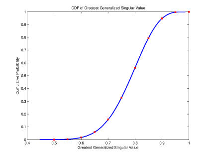
Figure 1: Empirical vs. analytic when $m=7$, $n=4$, $p=5$, $\beta=2.5$, and $\Omega={\rm diag}(1,2,2.5,2.7)$.

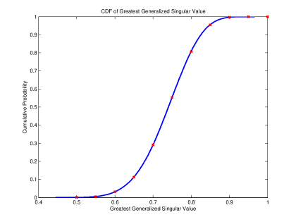
Figure 2: Empirical vs. analytic when $m=9$, $n=4$, $p=6$, $\beta=3$, and $\Omega={\rm diag}(1,2,2.5,2.7)$.

References

• [1] Ioana Dumitriu and Alan Edelman, β€œMatrix models for beta ensembles,” Journal of Mathematical Physics, Volume 43, Number 11, November, 2002.
• [2] Ross A. Lippert, β€œA matrix model for the $\beta$-Jacobi ensemble,” Journal of Mathematical Physics, Volume 44, Number 10, October, 2003.
• [3] Rowan Killip and Irina Nenciu, β€œMatrix Models for Circular Ensembles,” International Mathematics Research Noticies, No. 50, 2004.
• [4] Peter J. Forrester, Eric M. Rains, β€œInterpretations of some parameter dependent generalizations of classical matrix ensembles,” Probability Theory and Related Fields, Volume 131, Issue 1, pp. 1-61, January, 2005.
• [5] Alan Edelman and Brian D. Sutton, β€œThe Beta-Jacobi Matrix Model, the CS Decomposition, and Generalized Singular Value Problems,” Foundations of Computational Mathematics, 259-285 (2008).
• [6] Ioana Dumitriu and Plamen Koev, β€œDistributions of the extreme eigenvalues of Beta-Jacobi random matrices,” SIAM Journal of Matrix Analysis and Applications, Volume 30, Number 1, 2008.
• [7] Peter J. Forrester, β€œProbability densities and distributions for spiked Wishart $\beta$-ensembles,” 2011, http://arxiv.org/abs/1101.2261
• [8] Alexander Dubbs, Alan Edelman, Plamen Koev, and Praveen Venkataramana, β€œThe Beta-Wishart Ensemble,” 2013, http://arxiv.org/abs/1305.3561
• [9] R. A. Fisher, β€œThe sampling distribution of some statistics obtained from non-linear equations,” Ann. Eugenics 9, 238-249, 1939.
• [10] P. L. Hsu, β€œOn the distribution of roots of certain determinantal equations,” Ann. Eugenics 9, 250-258, 1939.
• [11] S. N. Roy, β€œp-Statistics and some generalizations in analysis of variance appropriate to multivariate problems,” Sankhya 4, 381-396, 1939.
• [12] A. G. Constantine, β€œSome non-central distribution problems in multivariate analysis,” Ann. Math. Statist. Volume 34, Number 4, (1963).
• [13] Alan T. James, β€œDistributions of matrix variates and latent roots derived from normal samples,” Ann. Math. Statist. Volume 35, Number 2, (1964).
• [14] Plamen Koev and Alan Edelman, β€œThe Efficient Evaluations of the Hypergeometric Function of a Matrix Argument,” Mathematics of Computation, Volume 75, Number 254, Pages 833-846, January 19, 2006. Code available at http://www-math.mit.edu/Β plamen/software/mhgref.html
• [15] Alan Edelman, β€œThe random matrix technique of ghosts and shadows,” Markov Processes and Related Fields, 2010.
• [16] I. G. Macdonald, β€œHypergeometric functions,” unpublished manuscript.
• [17] T. H. Baker, P. J. Forrester, β€œThe Calogero-Sutherland Model and Generalized Classical Polynomials,” Communications in Mathematical Physics, Volume 188, Issue 1, September, 1997.
• [18] Jyoichi Kaneko, β€œSelberg integrals and hypergeometric functions associated with Jack polynomials,” SIAM Journal on Mathematical Analysis, Volume 24, Issue 4, July 1993.
• [19] P. J. Forrester, Log-Gases and Random Matrices, London Mathematical Society Monographps Series, vol. 34, Princeton University Press, Princeton, NJ, 2010.
• [20] Ioana Dumitriu, Alan Edelman, Gene Shuman, β€œMOPS: Multivariate orthogonal polynomials (symbolically),” Journal of Symbolic Computation, Volume 42, Issue 6, June, 2007.
• [21] George E. Andrews, Richard Askey, and Ranjan Roy, Special Functions, Cambridge University Press, 1999.