A RAVE investigation on Galactic open clusters
I. Radial velocities and metallicities

Abstract

Context. Galactic open clusters (OCs) mainly belong to the young stellar population in the Milky Way disk, but are there groups and complexes of OCs that possibly define an additional level in hierarchical star formation? Current compilations are too incomplete to address this question, especially regarding radial velocities (RVs) and metallicities ($[M/H]$).

Aims. Here we provide and discuss newly obtained RV and $[M/H]$ data, which will enable us to reinvestigate potential groupings of open clusters and associations.

Methods. We extracted additional RVs and $[M/H]$ from the RAdial Velocity Experiment (RAVE) via a cross-match with the Catalogue of Stars in Open Cluster Areas (CSOCA). For the identified OCs in RAVE we derived $\overline{RV}$ and $\overline{[M/H]}$ from a cleaned working sample and compared the results with previous findings.

Results. Although our RAVE sample does not show the same accuracy as the entire survey, we were able to derive reliable $\overline{RV}$ for 110 Galactic open clusters. For 37 OCs we publish $\overline{RV}$ for the first time. Moreover, we determined $\overline{[M/H]}$ for 81 open clusters, extending the number of OCs with $\overline{[M/H]}$ by 69.

1 Introduction

Open clusters (OCs) are birthplaces of stars (Lada & Lada 2003; Lada 2006) and serve as convenient tracers of the young stellar population (age $\lesssim$ 2 Gyr) in the Galactic disk. Because OCs can harbour up to a few thousand stars, certain parameters, such as age, distance, and velocities, can be derived more accurately for OCs than for isolated stars. In general, OC members are selected from kinematics, that is, sharing a common motion (mainly proper motion is used), and photometry, that is, following the same isochrone in the colour-magnitude diagram. Cluster samples, reliably cleaned from fore- and background stars, are ideal targets for systematic investigations of stellar systems and the Milky Way as a whole regarding structure, dynamics, formation, and evolution.
Throughout the past decades several comprehensive studies, observational and literature compilations, were carried out to identify and characterise Galactic OCs. One important study was conducted by Lyngå (1987), providing a catalogue of 1151 OCs partly equipped with distances, ages, and even more sparsely with metallicities. It is often referred to as the Lund catalogue. Another set of catalogues was provided by Ruprecht et al. (1981), containing solely central coordinates and identifiers for 137 globular clusters, 1112 open clusters, and 89 associations.
The Two Micron All Sky Survey (2MASS; Cutri et al. 2003) provided a new source for cluster searches. Bica et al. (2003a, b) identified 276 infrared clusters and stellar groups as well as 167 embedded clusters related to nebulae. In addition to the identifiers and coordinates, they list angular sizes measured by eye. Dutra et al. (2003) extended these catalogues to the southern hemisphere by 123 clusters, providing the same type of information. Another extensive infrared OC catalogue in 2MASS was generated by Froebrich et al. (2007) near the Galactic disk $(|b|<20^{\circ})$. They provide coordinates, radii, and stellar densities for 1788 open and globular clusters, including 1021 new objects.
In the optical HIPPARCOS (Perryman et al. 1997) and TYCHO-2 (Høg et al. 2000) provided another opportunity for OC searches. Platais et al. (1998) published positions, distances, diameters, ages, and proper motions for 102 clusters and associations in HIPPARCOS, including 82 known objects and 20 new discoveries. Alessi et al. (2003) detected 11 new OCs in the TYCHO-2 data and list positions, diameters, distances, ages, proper motions, and velocity dispersions.
Currently, most known OCs are summarised in two main online compilations. One is the collection of optically visible open clusters and candidates by Dias et al. (2002) (hereafter referred to as DAML). It contains all available parameters, such as positions, radii, distances, ages, and proper motions for 2174 open clusters, including a few associations. Radial velocities (RVs) are given for 542 listings (25%), and metallicities ($[M/H]$) or iron abundances ($[Fe/H]$) for 201 clusters (9%). The second is the WEBDA data base created by Mermilliod (1988) and maintained by Netopil et al. (2012), collecting information on 970 Galactic OCs and 248 OCs in the Small Magellanic Cloud. For the Galactic OCs they list positions, diameters, distances, ages, proper motions, RVs, and colour excess, if available. The vast majority of WEBDA entries (910) is included in the DAML.
These compilations are essential for comprehensive studies, being the most complete collections of open clusters and associations. However, the information therein is highly inhomogeneous, due to different data sources and algorithms used for the membership selection and parameter determination. Furthermore, the provided parameters were not transferred to a uniform reference system, which could induce additional systematic biases, which in turn could lead to false conclusions on the overall characteristics of the OC system.
Kharchenko et al. (2005a, b) presented the Catalogue of Open Cluster Data (COCD), comprising in total 650 Galactic open clusters and associations (OCs). The OCs were extracted from the DAML or were newly discovered by applying a uniform membership selection and are provided with a mostly homogeneous set of parameters. Kharchenko et al. (2007) extended the RV information in COCD, based on the second edition of the Catalogue of Radial Velocities with Astrometric Data (CRVAD-2; Kharchenko et al. 2007) and literature values. The results were published in the Catalogue of Radial Velocities of Open Clusters and Associations (CRVOCA; Kharchenko et al. 2007). Currently, this is the only global RV study for OCs.
Here we present an update and extension of RV and $[M/H]$ information on OCs in the southern hemisphere, using the RAdial Velocity Experiment (RAVE; Steinmetz et al. 2006). In a second publication (Conrad et al. in prep.) we will use these additional and mostly homogeneous data, along with previous results, to reinvestigate the proposed OC groups and complexes (Piskunov et al. 2006). This may give us a hint on how they formed.
This publication is structured as follows: in Sect. 2 we briefly describe all catalogues used throughout the paper. In Sect. 3 we give a detailed description of our quality requirements to ensure a good working sample and discuss the stellar parameters obtained for RAVE stars in OC areas. In Sect. 4 we present the cluster mean values, and in Sect. 5 we conclude with a discussion on our results and an outlook on our ongoing project.

2 Catalogues

2.1 Catalogue of Open Cluster Data

The All-Sky Compiled Catalogue of 2.5 million stars (ASCC-2.5; Kharchenko 2001) contains relatively bright stars (V_Johnson down to 12.5 mag) listed with proper motions. It was the source catalogue for compiling the Catalogue of Open Cluster Data (COCD; Kharchenko et al. 2005a, b). For the first part of the COCD Kharchenko et al. (2005a) identified ASCC-2.5 stars in areas around 520 OCs taken from DAML. An independent search for OCs in ASCC-2.5 by Kharchenko et al. (2005b) extended the COCD by 109 previously unknown and 21 additional DAML clusters. The complete COCD provides centre positions, core radii, tidal radii, distances, ages, and mean proper motions (PMs) for in total 650 OCs. Mean radial velocities ($\overline{RV}$s) are provided for about 50% of the listed objects.
In addition, Kharchenko et al. (2004b, 2005b) published corresponding stellar catalogues for both parts of COCD, called the Catalogue of Stars in Open Cluster Areas (CSOCA). It provides equatorial coordinates, proper motions, $B$ and $V$ magnitudes, angular distances to the OC centre, as well as RVs, trigonometric parallaxes, and spectral types, if available. For the membership selection Kharchenko et al. (2004b, 2005b) applied uniform procedures considering radial stellar density distributions, kinematics, and photometry, which typically converged after a few iterations and provided three membership probabilities.
The spatial membership probability ($P_{pos}$) was set to unity for objects within the OC radius and zero otherwise. The kinematic membership probability ($P_{kin}$) can take values of 0$-$100% and is higher for stars sharing the common motion of the corresponding OC. The photometric membership probability ($P_{phot}$) also covers the range 0$-$100% continuously and is higher for stars that are closer to the corresponding OC-isochrone in the colour-magnitude diagram. Stars with $P_{phot}$ and $P_{kin}\geq 61$% are called 1$\sigma$-members. Those with $P_{phot}$ and $P_{kin}\geq 14\%$ are referred to as 2$\sigma$-members and targets with $P_{phot}$ and $P_{kin}\geq 1\%$ are considered as 3$\sigma$-members.
Moreover, CSOCA lists variability and binarity flags mainly from TYCHO-1 and -2 (Høg et al. 1997, 2000), HIPPARCOS (Perryman et al. 1997), CMC (Fabricius 1993), GCVS (Samus et al. 1997), NSV (Kazarovets et al. 1998), and PPM (Röser & Bastian 1991; Bastian & Röser 1993). The GCVS/NSV flags only indicate whether a star is variable or not, but do not specify the variability type. The CMC variability flag also does not provide specify the variable type, but gives information on insufficient or missing magnitudes. The PPM binarity flag again only indicates binary candidates, but does not provide additional information on the system. More detailed information on variability and binarity is provided by the TYCHO and HIPPARCOS flags. We found that about 10.4% of the CSOCA stars are provided with flags indicating variability and about 4.1% with flags indicating binarity. Among the flagged stars we found 3336 (1.7% of the CSOCA) that were indicated to be duplicity-induced variables.

2.2 Previous RV data

The RV data in CSOCA were obtained from the Catalogue of Radial Velocities with Astrometric Data (CRVAD; Kharchenko et al. 2004a), based primarily on the General Catalogue of mean Radial Velocities (Barbier-Brossat & Figon 2000). Kharchenko et al. (2007) updated the CRVAD to a second version (CRVAD-2) using additional stellar RVs from the Geneva-Copenhagen survey (Nordström et al. 2004), the Pulkovo Compilation of Radial Velocities (Gontcharov 2006) as well as CORAVEL and HIPPARCOS/TYCHO-2 kinematics on K and M giants (Famaey et al. 2005).
Kharchenko et al. (2007) stated that only 71% of the CRVAD-2 entries are provided with RV uncertainties. Another 21.5% have RV quality indices from Dufolt et al. (1995), either indicating specific standard errors or insufficient data. Only nine stars in CRVAD-2 show flags indicating insufficient data, which is negligible compared with the 7.5% of CRVAD-2 entries with no available uncertainties. We updated the RVs in CSOCA with CRVAD-2 information and found that 5% of the 3$\sigma$-members, 6% of the 2$\sigma$-members, and 9% of the 1$\sigma$-members are equipped with RVs.
Kharchenko et al. (2007) updated the RV information in the COCD and presented their results in the Catalogue of Radial Velocities of Open Clusters and Associations (CRVOCA). It contains literature and self-computed $\overline{RV}$ for 516 open clusters and associations, containing 395 COCD objects. The calculated $\overline{RV}$ are based on potential cluster members with $P_{kin}$ and $P_{phot}\geq$ 1%. For 32 clusters they found no such potential member and took one star with $P_{kin}>$1% and its RV value as representative for the corresponding clusters. The literature values were obtained from DAML for clusters and from Melnik & Efremov (1995) for associations (for a detailed list of references see Kharchenko et al. 2007).
Only 177 CRVOCA objects have both computed and literature values and agree well (see Fig. 2 in Kharchenko et al. 2007). Of the 395 COCD clusters in CRVOCA, 363 have calculated $\overline{RV}$. The remaining 32 OCs are provided with only literature values. Currently, the CRVOCA provides the most homogeneous RV reference sample for Galactic open clusters.

2.3 Previous abundance data

The COCD itself does not provide any metallicity information for OCs. Dias et al. (2002), on the other hand, provided metallicities or iron abundances for 96 COCD objects. Only 20 COCD entries have abundance values derived from more than five individual measurements. The abundance uncertainties in DAML can reach 0.2 dex.
Dias et al. (2002) did not separate between mean metallicity ($[M/H]$) and iron abundance ($[Fe/H]$), but gave information on the photometric or spectroscopic technique used to derive the values and literature references. When the abundance is directly derived spectroscopically from iron lines, we consider it representative for $[Fe/H]$, otherwise we expect it to be representative for $[M/H]$. When no information on the technique or literature reference was given in DAML, we assumed the value to refer to $[M/H]$. Although the DAML metallicities are inhomogeneous, they provide a sufficient reference sample with acceptable uncertainties.

2.4 RAdial Velocity Experiment

The RAdial Velocity Experiment (RAVE; Steinmetz et al. 2006) is a spectroscopic stellar survey in the southern hemisphere, observing primarily at high Galactic latitudes. The data were obtained with the six-degree field (6dF) instrument at the Anglo-Australian Observatory, providing mid-resolution (R$=$7500) spectra in the spectral range of the CaII-triplet (8410$-$8795Å). In addition to photometry from TYCHO-2 (Høg et al. 2000), the DEep Near-Infrared southern sky Survey (DENIS; Epchtein et al. 1997) and 2MASS (Cutri et al. 2003), RAVE provides RVs, $[M/H]$, surface gravities ($\log g$), and effective temperatures ($T_{eff}$) along with spectral quality parameters and flags.
Throughout the data releases the calibrations, especially regarding spectral parameters, were changed slightly. For details see the RAVE data release papers (Steinmetz et al. 2006; Zwitter et al. 2008; Siebert et al. 2011; Kordopatis & the RAVE Collaboration 2013). For our project we used results from the most recently improved pipeline of RAVE DR4, containing in total 482430 entries for 425561 stars. DR4 combines pipeline results from DR3 with new stellar parameters from Kordopatis & the RAVE Collaboration (2013). In addition, spectral classification flags by Matijevič et al. (2012) are included.
In RAVE studies on spectroscopic binaries were carried out by Matijevič et al. (2010, 2011). Based on multiple measurements for about 8.7% of DR3 stars, Matijevič et al. (2011) identified 1333 stars (6.6% of RAVE DR3) with significantly varying RV data, which indicated them to be single-lined spectroscopic binaries (SB1). These authors also stated that for larger numbers of repetitions (five or six measurements) the binary fraction for SB1 increases to about 10-15%, which they referred to as the lower limit for the binary fraction in RAVE.
Matijevič et al. (2010), on the other hand, investigated the cross-correlation function of observed to template spectra (Munari et al. 2005) in DR2. They identified 123 double-lined spectroscopic binaries (SB2), indicated either by more than one peak or an asymmetric central peak. From simulations, Matijevič et al. (2010) concluded that RAVE should be able to detect more than 2000 SB2 binaries. In their recent work, Matijevič et al. (2012) not only updated the SB2 list, but also provided quality flags on RAVE spectra. These indicate problematic spectral features that might affect the reliability of the stellar parameters.

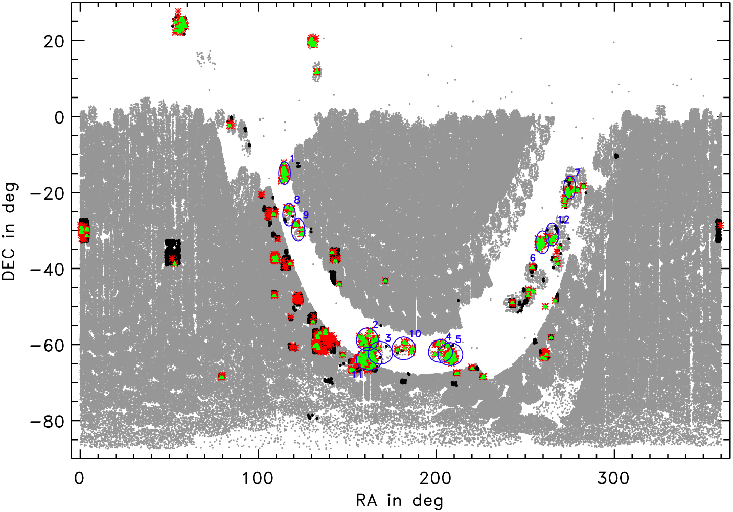
Figure 1: Spatial distribution of stars in OC areas covered by RAVE. Black dots represent our high-quality RV sample. The entire RAVE DR4 is underlayed in grey. The good and best RV members are overplotted as red asterisks and green triangles, respectively. The 12 dedicated OC fields are highlighted by blue circles.

2.5 Dedicated OC observations in RAVE

In 2004, members of our research group proposed 12 observing fields to RAVE located in the Galactic plane (see Fig. 1). Each field contains at least 100 stars, and fields with more than 150 targets were suggested to be observed repeatedly with different fibre configurations to avoid allocation problems due to crowding. In total our dedicated OC fields in RAVE cover about 1500 stars in areas around 85 known open clusters (OC areas), including about 400 stars with known RVs from CRVAD-2 to ensure reliable $\overline{RV}$ determination for the observed OC. The observation sample was compiled from stars fainter than 9 mag in the SSS $I$-band with no bright object within a radius of 10″and no star brighter than $I=$16 mag within a radius of 8″. The flux contamination of stars fainter than $I=$16 mag within a radius of 8″of the bright main target can be considered negligible. Hence, these objects were included in the observing sample. Up to the present, the overall number of OC areas covered by RAVE has increased by almost a factor of three with respect to the 85 proposed areas, due to additional observations in regions around known OCs.

3 Stellar parameters for stars in OC regions observed by RAVE

3.1 Sample selection and data quality

To set up our working sample, we first updated the RV information in CSOCA with values from CRVAD-2 and then cross-matched the RV-updated CSOCA with RAVE DR4 based on a coordinate comparison with a search radius of 3″. The spatial distribution of all COCD objects identified in RAVE is displayed in Fig. 1, with the 12 dedicated OC fields highlighted. The majority of our OCs are located in or near the Galactic plane ($|b|\leq$ 20 deg), usually avoided by RAVE.
In addition to the 85 OC areas from the dedicated cluster observations, we found 159 more regions covered by RAVE. In total, we identified 6402 measurements of 4865 stars in 244 OC areas, all equipped with RV information in RAVE. We refer to this as our RV sample. Since $[M/H]$ determination requires spectra of higher quality, our metallicity sample comprises 6209 measurements of 4785 stars in 244 OC areas.
These two samples solely result from the cross-match between CSOCA and RAVE and still contain data of insufficient quality. To ensure good data quality in our working sample, we applied several constraints in RAVE quality parameters and spectral classification flags. As a final step we included OC membership probabilities in our list of requirements to clean the working sample from non-members.

Quality cut in signal-to-noise

One obvious parameter to define quality constraints is the spectral signal-to-noise ratio. Throughout this paper we use the listed SNR value in RAVE DR4 and show the distribution of RV uncertainties ($eRV^{*}$) with respect to the SNR in Fig. 2.
For the entire RAVE DR4 the distribution is very random. To better identify the overall trend we computed the median in $eRV^{*}$ ($\epsilon RV$) in bins along the SNR. For an SNR $<$ 100 we chose a bin size of 4 and for an SNR $\geq$ 100 we changed it to 10, to include a sufficient number of data points. Typically, the overall trend is very flat and well below 5 km/s. Only for an SNR $\leq$ 10 a significant increase in $\epsilon RV$ is present. Thus, we defined our first cut at an SNR $\geq$ 10.

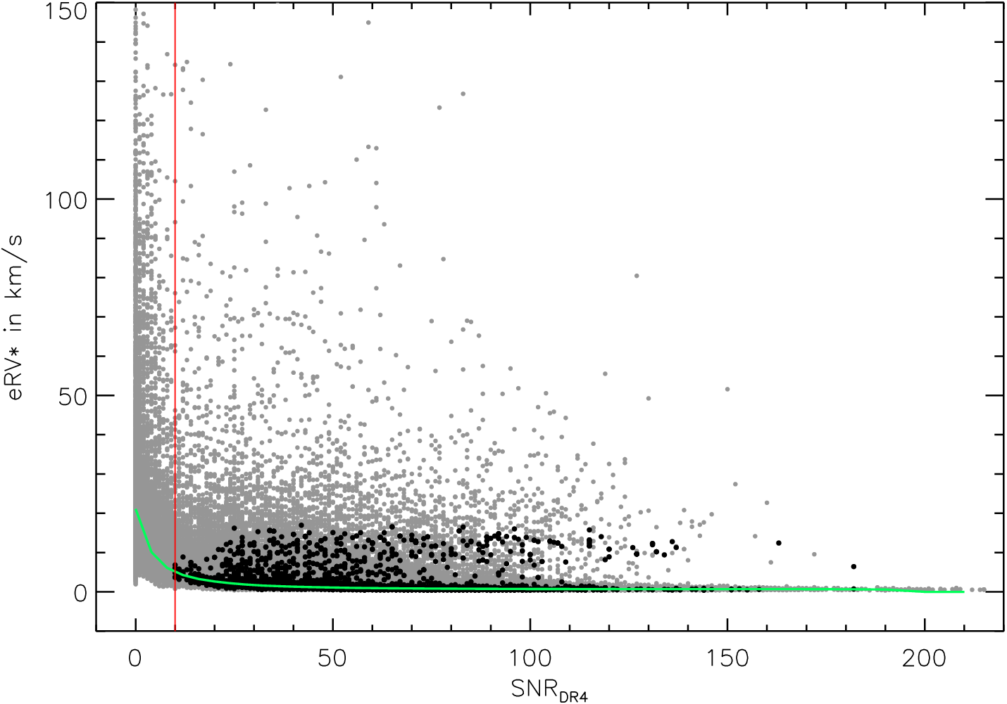
Figure 2: $eRV^{*}$ vs. SNR distribution in RAVE DR4 (grey dots). Black dots show our high-quality RV sample. The green and red solid lines give the $\epsilon RV$ trend and cut at an SNR $\geq$ 10, respectively.

Quality cut in the spectral correlation coefficient

However, even at high SNR ($\geq$ 50) a considerable fraction of RAVE entries show $eRV^{*}$ of up to 40 km/s, making additional quality requirements necessary. Therefore, we checked the correlation coefficient ($R$), which characterises the goodness-of-match between the observed and the template spectrum. The better the match, the higher is $R$, and the more reliable are the derived stellar parameters.
The $eRV^{*}$ vs. $R$ distribution (Fig. 3) is much tighter and appears to be more suited to ensure well-measured RV data than the SNR. Again we computed the overall trend in DR4 as $\epsilon RV$ in bins of 4 along $R$. At $R<$ 10 the overall trend shows a significant increase, indicating poorly determined stellar parameters. Our second cut at $R\geq$ 10 cleans our working sample from these unreliable targets and ensures $eRV^{*}\leq 20$ km/s.

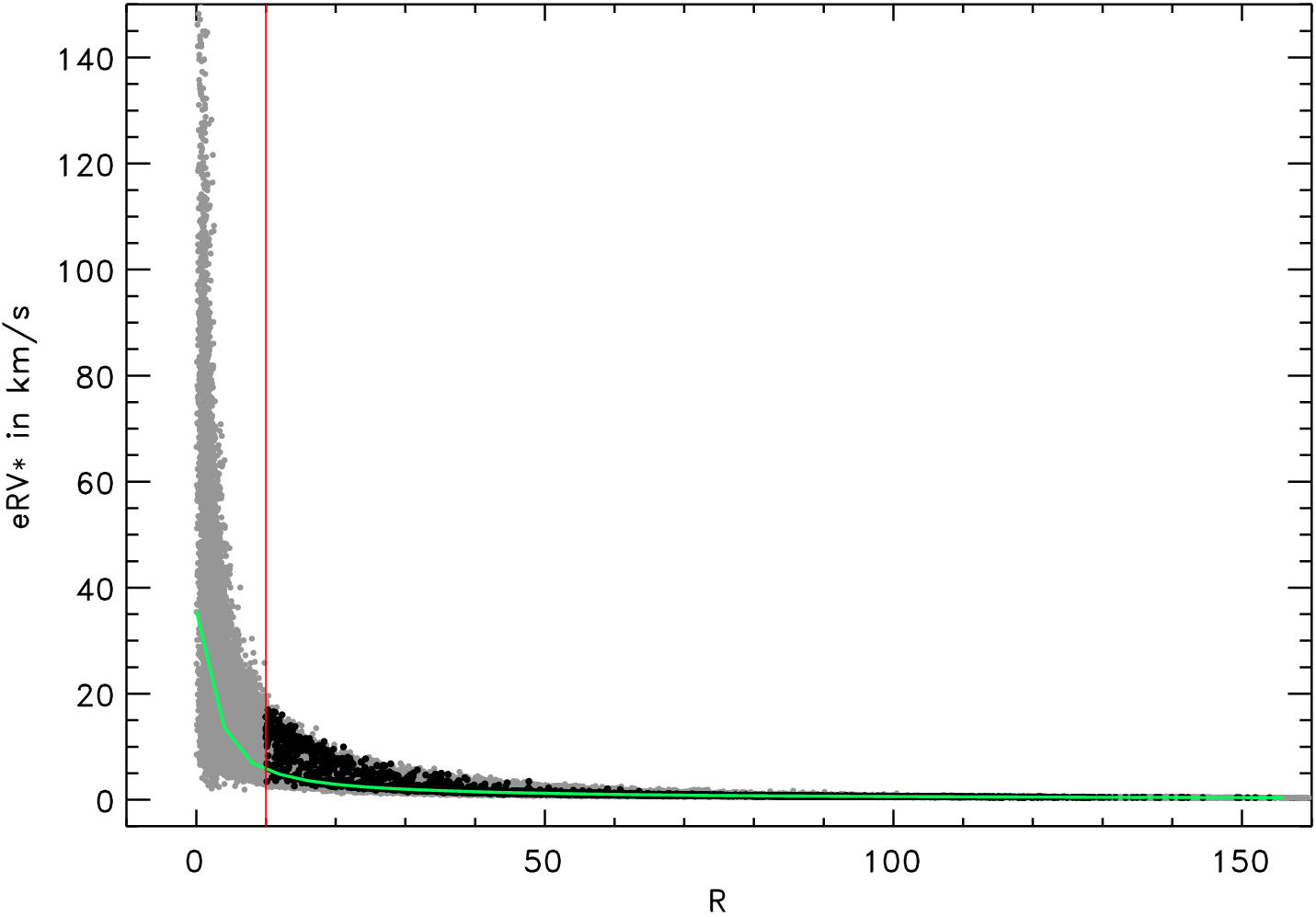
Figure 3: $eRV^{*}$ vs. $R$ distribution in RAVE DR4 (grey dots) and our high-quality RV sample (black dots). The green and red solid lines represent the $\epsilon RV$ trend and our cut at $R\geq$ 10, respectively.

Quality cut in the RV correction parameter

Moreover, RAVE provides RV corrections ($corr\_RV$) based on systematic effects (for details see Steinmetz et al. 2006; Zwitter et al. 2008; Siebert et al. 2011). The effect of $corr\_RV$ on the data quality, especially regarding radial velocities, is shown as the $eRV^{*}$ vs. $corr\_RV$ distribution in Fig. 4.
Apparently, $corr\_RV$ can increase to 50 km/s and the distribution becomes more clumpy for higher $corr\_RV$ values. This is seen even for stars that match the first two criteria (SNR $\geq$ 10 and $R\geq$ 10). Thus, our third cut we defined as $|corr\_RV|\leq$ 9 km/s, where the distribution is very smooth.

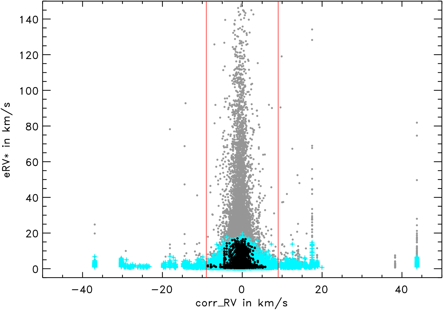
Figure 4: $eRV^{*}$ vs. $corr\_RV$ distribution in RAVE DR4 (grey dots). Cyan crosses illustrate the subsample that matches an SNR $\geq$ 10 and $R\geq$ 10. Black dots show our high-quality RV sample and the red solid lines illustrate our cuts at $|corr\_RV|\leq$ 9 km/s.

Table 1: Numbers for our different RV samples in RAVE and OC areas.

	RAVE DR4		OC sample
Number of	entire	high-quality	RV	high-quality	good RV	best RV
	RAVE	in RAVE	sample	RV sample	members	members
Measurements	483849	405944	6402	4768	764	520
Stars	426945	366922	4865	4064	664	443
Clusters	—	—	244	217	120	105

Spectral flags and OC membership

The study on the morphology of RAVE spectra by Matijevič et al. (2012) provides quality flags for the majority of RAVE spectra. The flags indicate SB2 binaries, too cool or too hot stars, problematic spectral features, and reliable spectra. If an object is flagged reliable, we considered it for our working sample. If the RAVE target is not classified at all, we only applied the quality constraints defined earlier (SNR $\geq$ 10, $R\geq$ 10 and $|corr\_RV|\leq$ 9 km/s). These four constraints define our high quality RV sample in OC areas covered by RAVE.
Since we aim to investigate open clusters, we have to take into account the membership probabilities as well. Primarily we used $1\sigma$-members, and combined with the previous requirements, we refer to these as our best RV members. In certain cases we also included $2\sigma$-members, which we call our good RV members.
In Tab. 1 we summarise the samples considered in this work. Only about 1% of the RAVE DR4 stars are located in OC areas from COCD and only 37.5% of the COCD clusters are covered by RAVE. After applying all quality requirements, we can only use about 12% of the RAVE stars in OC areas to calculate $\overline{RV}$. The resulting OC sample is still larger than the sample covered by the dedicated RAVE cluster fields.

Additional quality checks

To better characterise our working samples we checked the distribution of $eRV^{*}$ for our different samples (Fig. 5). Since the size of each sample is different, we normalised each histogram by the corresponding total number of measurements to make them comparable. As we expected, all histograms peak at about 1 km/s. However, $eRV^{*}$ below 1 km/s, as present in Fig. 5, are too optimistic, and especially for computing the $\overline{RV}$ we set all these very low $eRV^{*}$ to 1 km/s. Our good and best RV members show a significant fraction of measurements with $eRV^{*}>$ 3 km/s and therefore do not reflect the quality of the entire RAVE survey; yet we have to identify the reason for this finding.

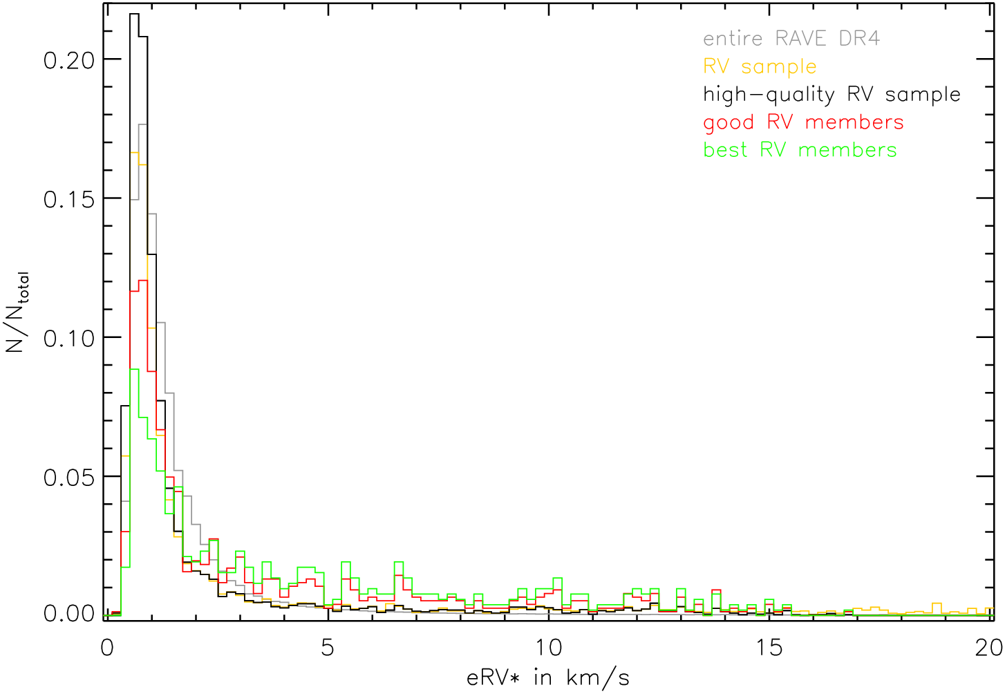
Figure 5: Histograms for $eRV^{*}$ for the entire RAVE DR4 (grey), our RV sample (yellow), our high-quality RV sample (black), and our good (red) and best (green) RV members.

First, we checked for a possible relation between the $eRV^{*}$ and RAVE observing date. In Tab. 2 we list the number of entries and $\epsilon RV$ in each observing year for our best RV members and the entire RAVE DR4 for comparison. The majority of best RV members (394 out of 520 measurements) were observed in 2004, 2005, and 2010. The corresponding $\epsilon RV$ are about a factor of 4 higher than the values of the remaining years. This is a specific feature of our OC member sample, since for the entire RAVE the $\epsilon RV$ are almost equal for all observing years. Although we can now relate the less accurate RVs of our best RV members to certain RAVE observing years, we cannot sufficiently explain the difference in data quality between RAVE and our good and best RV members.

Table 2: Comparison of $\epsilon RV$ between our best RV members and RAVE for each observing year.

	best RV members		entire RAVE
Observing	No. of	$\epsilon RV$	No. of	$\epsilon RV$
year	entries	in km/s	entries	in km/s
2003	0	—	19164	1.90
2004	109	4.51	28924	1.67
2005	104	4.20	30889	1.56
2006	9	1.64	78493	1.22
2007	18	0.88	53899	1.20
2008	18	1.13	60387	1.06
2009	15	1.11	75465	1.03
2010	181	4.47	59192	1.08
2011	20	0.87	50576	1.04
2012	46	1.66	25441	1.15
2013	0	—	1419	1.40
total	520	3.03	483849	1.18

To check for the degree of magnitude dependence in $eRV^{*}$, we show the magnitude-separated $eRV^{*}$ histograms for our high-quality RV sample in Fig. 6 and give the corresponding numbers of measurements and $\epsilon RV$ in Tab. 3. For $8-12$ mag the $\epsilon RV$ are almost equal, only for the faintest magnitude interval the $\epsilon RV$ value is about 0.5 km/s higher, as seen in Fig. 6 as well. Since the change in $eRV^{*}$ is only 0.5 km/s, the magnitude dependence can be considered negligible in our working sample.

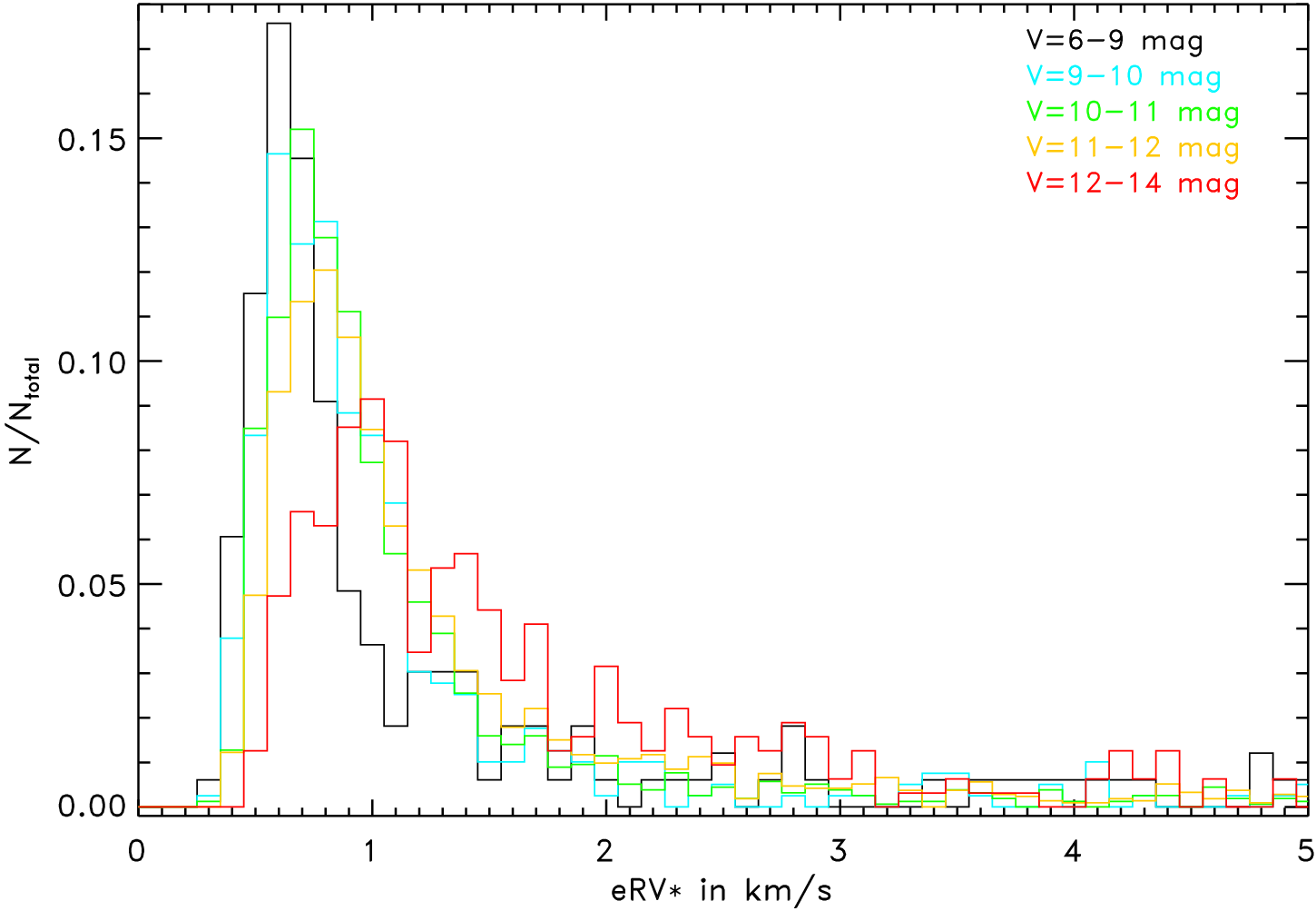
Figure 6: Magnitude-dependent $eRV^{*}$ histograms for our high-quality RV sample. The $V_{Johnson}$ intervals are 6-9 mag (black), 9-10 mag (blue), 10-11 mag (green), 11-12 mag (yellow), and 12-14 mag (red).

Open clusters are relatively young objects and are expected to be dominated by dwarfs. In our samples we separated dwarfs from giants based on $\log{g}$ in RAVE DR4. We considered giants to have $\log{g}<$ 3.75 dex and dwarfs to show $\log{g}\geq$ 3.75 dex. Objects with no $\log{g}$ were not included in this separation. The DR4 pipeline providing $\log{g}$, $T_{eff}$ and $[M/H]$ also list flags indicating potential problems in the convergence of the algorithm. Targets indicated to not converge or that had to be rerun were excluded from the $\log{g}$ separation. Thus, the number of dwarfs and giants in Tab. 3 does not necessarily add up to the total number of measurements in the corresponding magnitude bin.
In Tab. 3 we summarise the results for our high-quality RV sample and our good RV members. By total numbers the high-quality RV sample is dominated by giants with a giant-to-dwarf ratio of 2.96, while the good RV members contain an almost equal number of dwarfs and giants, showing a ratio of 1.08. These numbers confirm our expectation that OCs contain a larger number of dwarfs and that RAVE preferably observes giants.
Considering each magnitude interval, this becomes even more evident, because the number of good RV members that are dwarfs in $6\leq V_{Johnson}<11$ mag is higher than the number of giants, and for $11\leq V_{Johnson}\leq 14$ mag the number of dwarfs and giants are almost equal for the good RV members. In all magnitude intervals the $\epsilon RV$ of our good RV members are higher than the respective values in our high-quality RV sample, indicating a potential relation between stellar type and $eRV^{*}$.

Table 3: Number of entries, giant-to-dwarf ratios, and $\epsilon RV$ in magnitude intervals as shown in Fig. 6 for our high-quality RV sample and good RV members.

$V_{Johnson}$	high-quality RV sample			good RV members
in mag	No.	G/Da	$\epsilon RV$	No.	G/Da	$\epsilon RV$
6-9	193	110/    78	0.95	34	10/  23	3.79
9-10	472	261/  186	1.01	49	18/  29	1.83
10-11	1582	1231/  243	0.92	136	51/  74	1.50
11-12	2170	1505/  477	1.03	419	224/150	1.45
12-14	350	175/  123	1.48	126	50/  52	2.63
total	4768	3282/1108	1.00	764	353/328	1.73
aG/D - giant-to-dwarf ratio.

To investigate this aspect in more detail, we display the $eRV^{*}$ vs. $\log{g}$ diagram in Fig. 7. The pillar-like features in the $\log{g}$ distribution are due to the grid of synthetic spectra used to derive stellar parameters in RAVE DR4 (see Kordopatis et al. 2011; Kordopatis & the RAVE Collaboration 2013). We found that higher values of $\log{g}$ also show higher $eRV^{*}$. Potential reasons for this dependence could be that dwarfs show fewer and weaker absorption lines, which are used to derive RV. For our good and best RV members the effect of higher $eRV^{*}$ with higher $\log{g}$ appears to be stronger. Moreover, the location of our OCs in or near the Galactic disk might affect the quality of our working sample.

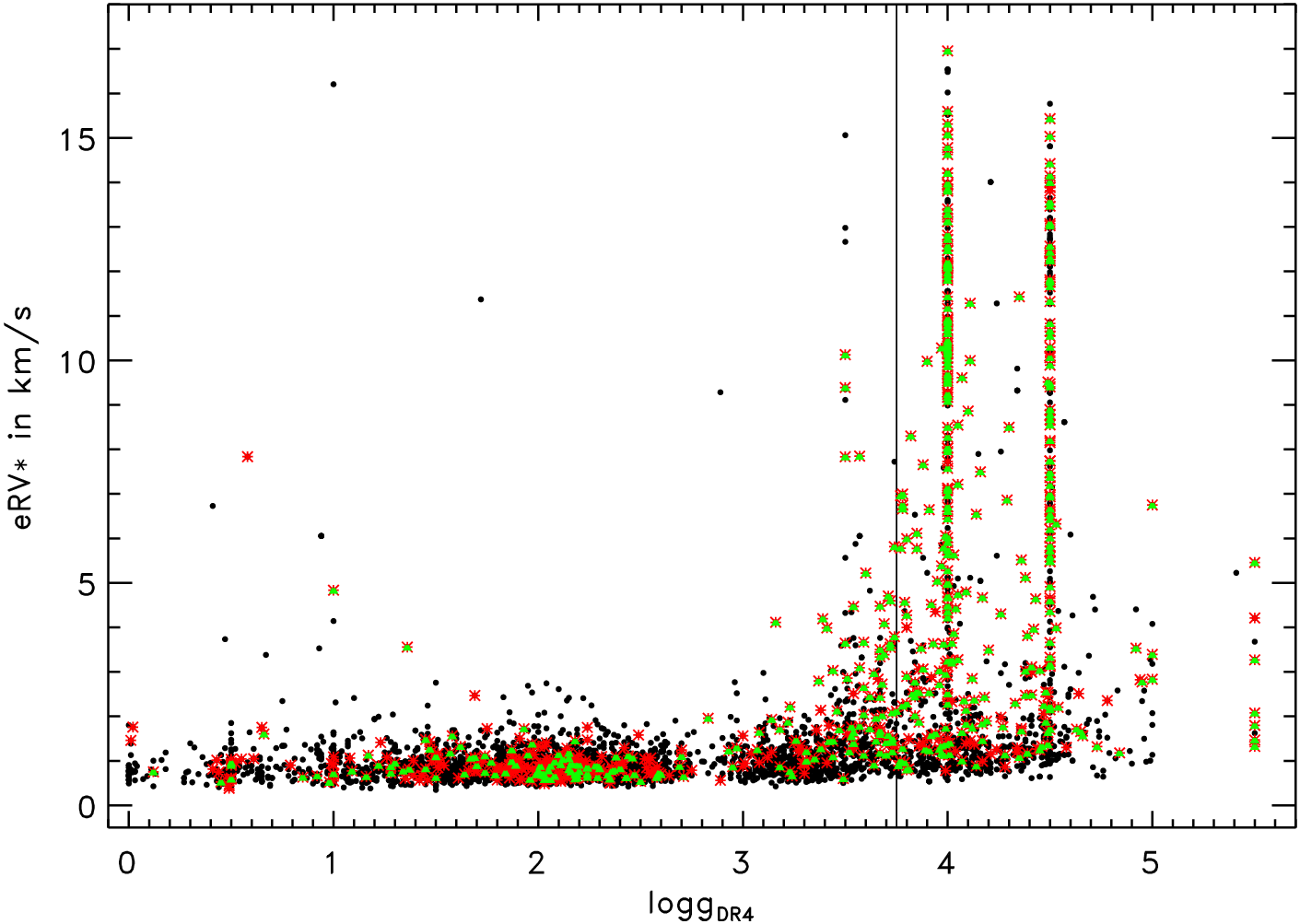
Figure 7: Distribution of $eRV^{*}$ with respect to $\log{g}$. Symbol colour-coding is the same as in Fig. 1. Our giant/dwarf separation limit at $\log{g}=3.75$ is included as the black solid line.

Therefore, we present the $eRV^{*}$ distribution with respect to the Galactic latitude ($b$) in the upper panel of Fig. 8. One can see that almost all good and best RV members with $eRV^{*}>5$ km/s are located very close to the Galactic plane. In the lower panel we show the $\log{g}$ vs. $b$ distribution and highlight all targets with $eRV^{*}>5$ km/s, which appear to be predominantly dwarfs. This confirms that the higher $eRV^{*}$ for our good and best RV members are mainly caused by the higher percentage of dwarfs in our OC sample. The possible effect of undetected binarity, extinction, or change in exposure time on $eRV^{*}$ we cannot study in detail with the data set used.

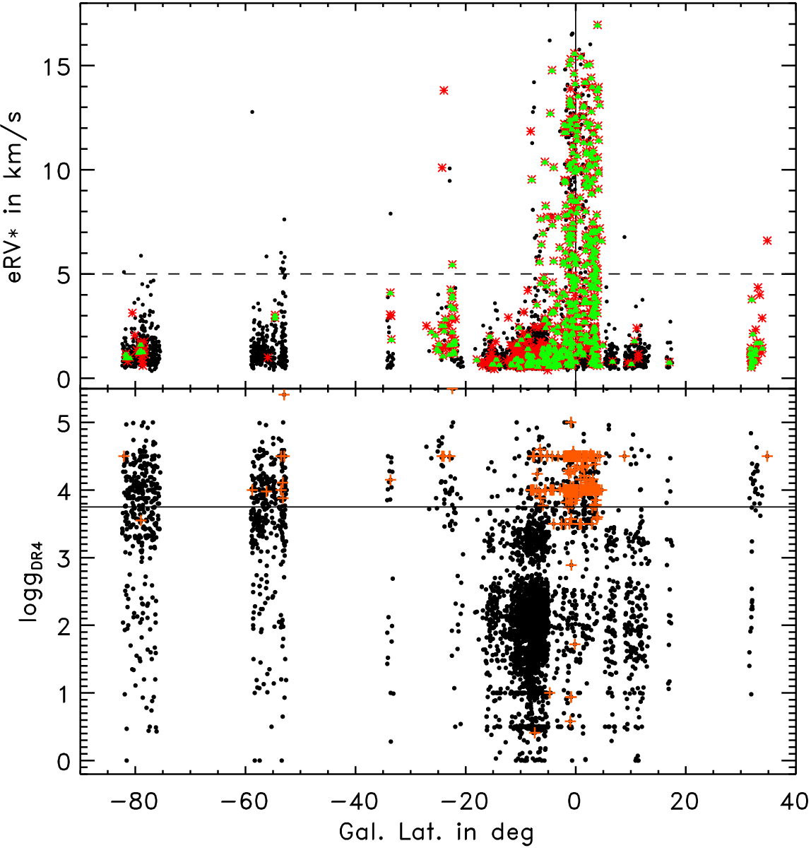
Figure 8: Distribution of $eRV^{*}$ and $\log{g}$ with respect to $b$ along with the mid-plane and $\log{g}$ limit (3.75) overplotted as the black solid line in the upper and lower panel, respectively. The symbol colour-coding is the same as in Fig. 1, and dark orange crosses highlight targets with $eRV^{*}>5$ km/s. This $eRV^{*}$ limit is displayed as the black dashed line.

We can conclude that even though our OC sample in RAVE does not reflect the accuracy of the entire survey, the quality of our working sample is still sufficient for our purposes , which are determining the average radial velocities ($\overline{RV}$) for open clusters.

Table 4: Comparison of numbers and RV uncertainties between RAVE, CRVAD-2, and the resulting common sample. The $\epsilon RV$ values are the median of the RV uncertainties and $\sigma\Delta RV$ correspond to the standard deviation of the difference distribution.

	Catalogues		OC sample
	entire	high-	RV	high-quality	good RV	best RV
		quality	sample	RV sample	members	members
— RAVE —
No. of entries	483849	405944	6402	4768	764	520
No. of clusters	—	—	244	217	120	105
$\epsilon RV$ in km/s	1.18	1.11	1.23	1.00	1.73	3.03
— CRVAD-2 —
No. of entries	54907	—	6782	—	1586	1092
No. of clusters	650	—	595	—	318	306
$\epsilon RV$ in km/s	0.86	—	3.60	—	3.70	3.70
— common sample —
No. of entries	2475	1774	531	262	51	32
No. of clusters	—	—	104	73	13	9
$\epsilon RV_{RAVE}$ in km/s	1.23	1.02	6.06	1.45	2.04	2.28
$\epsilon RV_{CRVAD-2}$ in km/s	0.60	0.50	2.90	1.80	1.70	1.70
$\sigma\Delta RV$ in km/s	90.66	22.65	81.21	38.20	22.75	21.02

3.2 Radial velocity

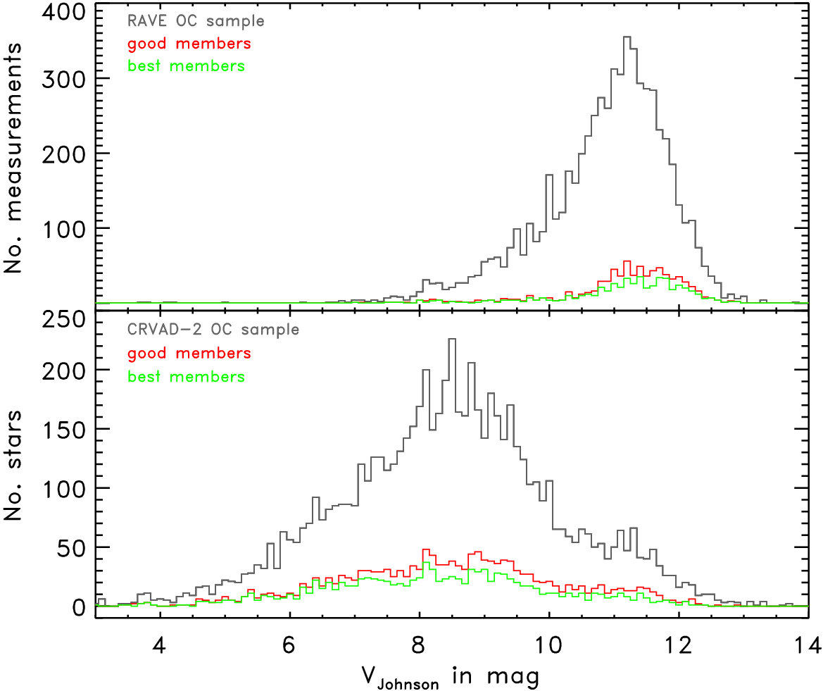
Figure 9: $V_{Johnson}$ histograms in RAVE (upper panel) and CRVAD-2 (lower panel) for objects in OC areas (grey), as well as our good (red) and best (green) RV members.

To better evaluate the RVs obtained by RAVE, we obtained reference values from CRVAD-2 and created a common sample for comparison via a cross-match based on coordinates with a matching radius of 3″. The numbers and $\epsilon RV$ for the two catalogues and the common sample are given in Tab. 4. The increase of $\epsilon RV$ after including membership probabilities, as stated above, is a RAVE-specific characteristic, since it is only present in the RAVE data, but not in CRVAD-2. For the good and best OC members with RV, on the other hand, the $\epsilon RV$ are similar in the two catalogues.
Interestingly, the common sample is very small (2500 listings) compared to the size of the two catalogues (RAVE: $\sim 460000$ entries and CRVAD-2: $\sim 55000$ stars) and only a very small fraction of objects in each catalogue is located within OC regions (about 1.3% in RAVE and about 12.3% in CRVAD-2). One reason for the small overlap between CRVAD-2 and RAVE is that each catalogue has different observing samples: RAVE is a southern-sky survey, while CRVAD-2 was an all-sky project.
Moreover, RAVE and CRVAD-2 cover different magnitude ranges shifted by almost 3 mag, as presented in Fig. 9, also showing that RAVE only covers fainter OC members. Within OC areas, on the other hand, the fraction of good and best members are comparably large, that is, in RAVE 12.3% of objects in OC areas are good members and in CRVAD-2 the corresponding percentage is 23.4%. This indicates that the majority of objects in OC regions, included in each catalogue, are at least good members.
For the high-quality common sample we display the RV comparison between RAVE and CRVAD-2 source catalogues in Fig. 10, along with the corresponding difference distribution. The RV differences were computed as $\Delta RV=RV_{CRVAD-2}-RV_{RAVE}$. Near $RV_{RAVE}=0$ km/s we found several stars with intrinsically higher $RV_{CRVAD-2}$ than $RV_{RAVE}$. For our good and best RV members this feature entirely disappears. In the difference distribution a slight negative slope is also visible in the high-quality sample. Our good and best RV members do not show this slope distinctly, since only two stars show significant differences, which could be by chance. The remaining good and best members, except for the two deviating ones, show a spread in the difference distribution of 20 km/s. Hence, our selected good and best RV members agree well with the reference values and show a sufficiently good quality to derive $\overline{RV}$ for OCs in RAVE.
Still, we have to understand the identified systematics of our high-quality sample (see Fig. 10). Accordingly, we investigated the major CRVAD-2 source catalogues, namely Nordström et al. (2004), Gontcharov (2006), and Barbier-Brossat & Figon (2000). The results are presented visually in Fig. 11 and in numbers in Tab. 5. The vast majority of CRVAD-2 values were obtained from Barbier-Brossat & Figon (2000) and Nordström et al. (2004). The displayed difference distributions in Fig. 11 are relatively broad and might include several outliers. Therefore, we applied a 3$\sigma$-clipping algorithm to identify the actual distribution characteristics and also included the results for the clipped distributions in Tab. 5 and Fig. 11.
In the difference distributions (clipped and unclipped) for reference values from Nordström et al. (2004) and Gontcharov (2006) the standard deviations in the high-quality sample are considerably lower than for the comparison with values from Barbier-Brossat & Figon (2000). Therefore, the reference values from the first two catalogues seem to be more reliable. Moreover, the systematic effect near $RV_{RAVE}=0$ km/s is visible in all source catalogues, whereas the possible negative slope only appears in the comparison of our high-quality sample with values from Barbier-Brossat & Figon (2000). Thus, we can conclude that the trend is not a feature induced by the RAVE data but by the reference values from Barbier-Brossat & Figon (2000).
Surprisingly, we found no good and best members in common with Nordström et al. (2004). Moreover, the number of common good and best RV members with Gontcharov (2006) is negligible, which in turn makes the questionable values by Barbier-Brossat & Figon (2000) the dominant source for RV references. However, their values are the best RV references for OCs available, and since our good and best RV members in RAVE show a better agreement with these references than the high-quality data, it indicates that our cuts are suitable for deriving reliable $\overline{RV}$ for our OC sample.

Table 5: Characteristics for the RV difference distributions between RAVE and the source catalogues in CRVAD-2 for the high-quality sample as well as for the good and best RV members in our common sample.

	No.	$\epsilon RV$	$\overline{\Delta RV}$	$\sigma\Delta RV$
high-quality sample	before 3$\sigma$-clipping
Nordström	825	0.40	-0.69	8.10
Gontcharov	93	0.60	-1.86	12.71
Barbier-Brossat	852	1.70	6.54	42.54
	after 3$\sigma$-clipping
Nordström	743	0.30	-0.36	1.78
Gontcharov	89	0.60	-0.18	3.82
Barbier-Brossat	728	1.70	-0.57	11.27
good RV members	before 3$\sigma$-clipping
Nordström	–	—	—	—
Gontcharov	5	0.40	-20.50	46.50
Barbier-Brossat	46	2.00	-4.77	18.93
	after 3$\sigma$-clipping
Nordström	–	—	—	—
Gontcharov	4	1.30	0.29	0.90
Barbier-Brossat	38	1.80	-0.66	4.04
best RV members	before 3$\sigma$-clipping
Nordström	–	—	—	—
Gontcharov	3	0.40	-34.42	59.96
Barbier-Brossat	29	1.80	-1.44	11.27
	after 3$\sigma$-clipping
Nordström	–	—	—	—
Gontcharov	2	1.50	0.20	0.30
Barbier-Brossat	26	1.70	0.79	3.12

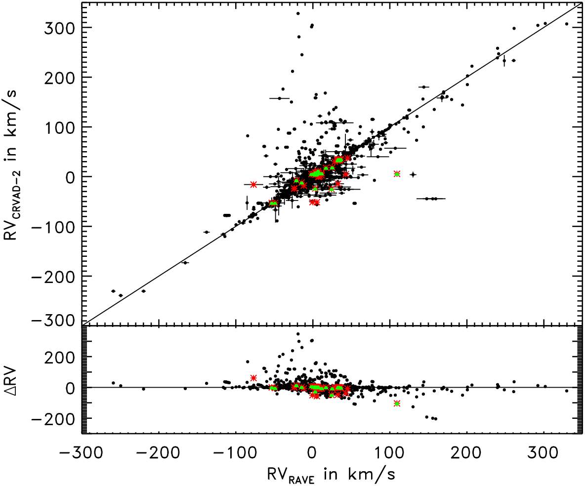
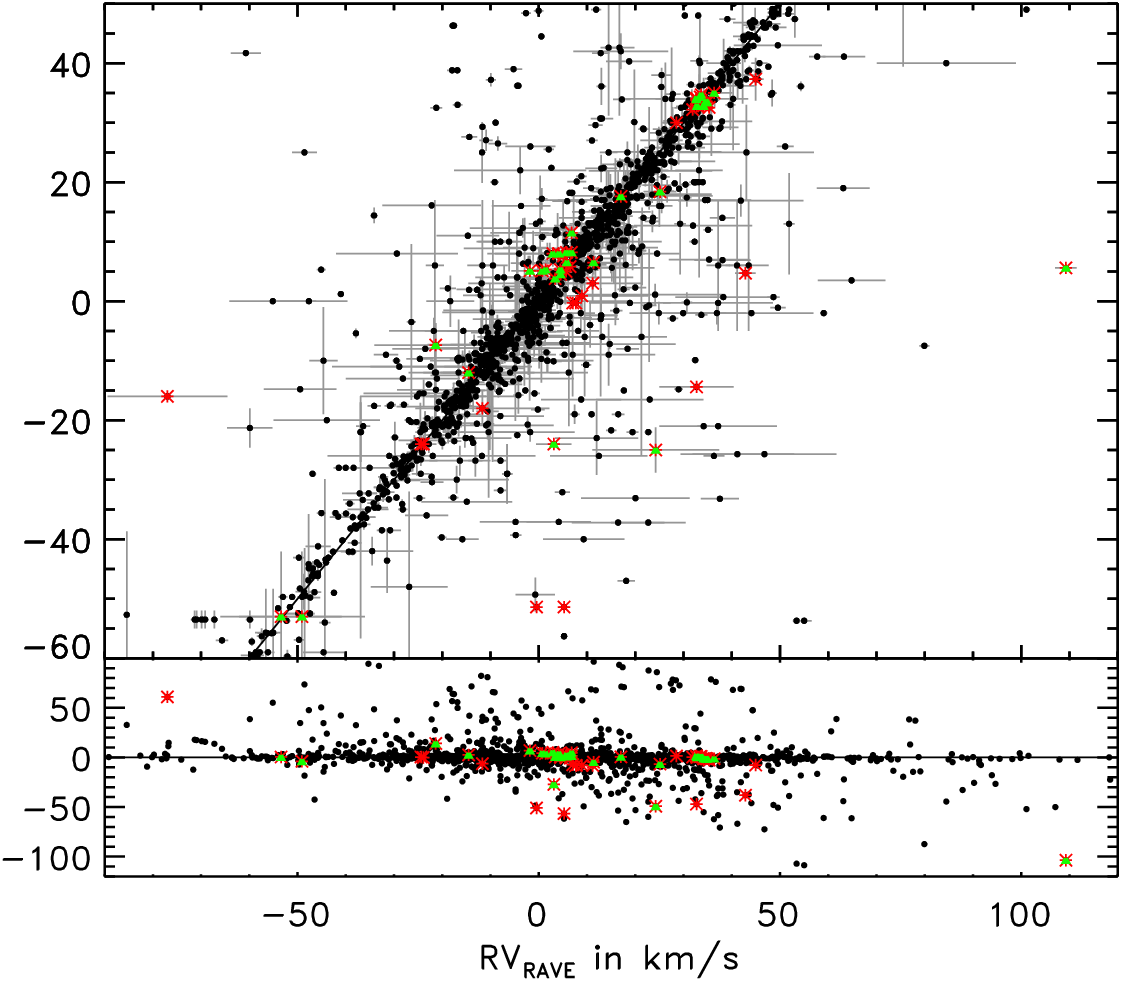
Figure 10: Upper panel: RV comparison between CRVAD-2 and RAVE. The black solid line refers to the one-to-one relation. Lower panel: Corresponding difference distribution along with the zero-difference line (black solid line). Black dots show the high-quality common sample, while red asterisks and green triangles highlight good and best RV members in the common sample, respectively. The right panels show the same diagrams enlarged to the RV range of our good and best RV members.

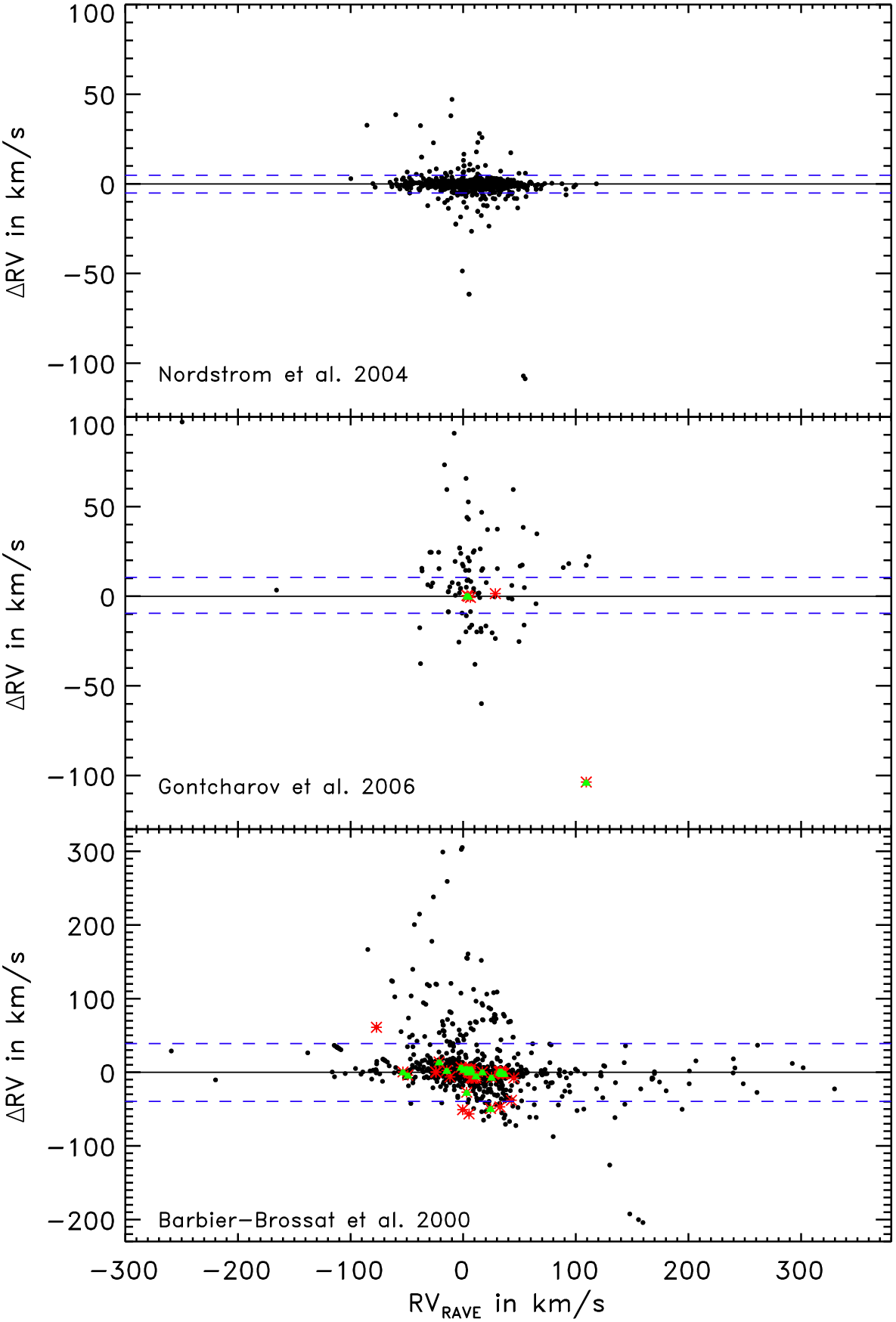
Figure 11: Unclipped RV difference distributions between RAVE and Nordström et al. (2004) (upper panel), Gontcharov (2006) (middle panel), and Barbier-Brossat & Figon (2000) (lower panel). The colour-coding is the same as in Fig. 10 and the blue dashed lines define the limits of the 3$\sigma$-clipped distributions.

3.3 Metallicity

We also aimed to provide mean metallicities ($\overline{[M/H]}$) for our RAVE clusters. Spectra of higher quality are typically needed for the metallicity determination and different template spectra were used than for deriving RVs. In DR4 Kordopatis & the RAVE Collaboration (2013) applied several prior constraints, namely SNR $\geq$ 20, $v_{rot}<$ 100 km/s, $eRV^{*}<$ 8 km/s, $logg>0.5$ and $T_{eff}>3800$ K. This resulted in a slightly smaller sample; 6209 out of the 6402 RAVE observations in OC regions are equipped with $[M/H]$ and we had to slightly adapt our quality constraints to conduct a reliable metallicity study. In addition, the DR4 pipeline provides quality flags for the convergence of the stellar parameter algorithm used to derive $\log{g}$, $T_{eff}$, and $[M/H]$. Since the RV values were derived by a different algorithm, we did not include them in our RV sample but have to do so now for our metallicity study. Objects with no converging algorithm or which had to be rerun by the pipeline were excluded from our metallicity study on open clusters.
As noted by Kordopatis & the RAVE Collaboration (2013), the internal metallicity uncertainties ($e[M/H]^{*}$) in RAVE DR4 were derived from different sets of synthetic spectra, leading to a discrete distribution (see Fig. 12). These $e[M/H]^{*}$ might reflect model errors instead of realistic measurement uncertainties. Therefore, we preferred to evaluate the actual $[M/H]$ values and not the uncertainties to define the adapted cuts for our metallicity study in open clusters.

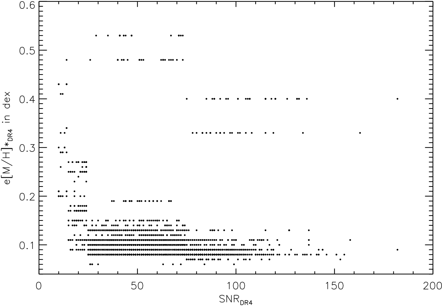
Figure 12: Distribution of $e[M/H]^{*}$ with respect to $SNR$ for our high-quality RV sample.

In Fig. 13 we display the $[M/H]$ distribution with respect to SNR. To illustrate the overall trend in RAVE DR4 we calculated $\overline{[M/H]}$ in bins of 4 along SNR and changed the bin size to 10 for SNR $\geq$ 100, to gain enough data points in each bin. This overall trend is quite flat and shows no specific correlation, not even for low SNR. Therefore, we simply adapted the same cut as the RAVE DR4 pipeline at an SNR $\geq$ 20.

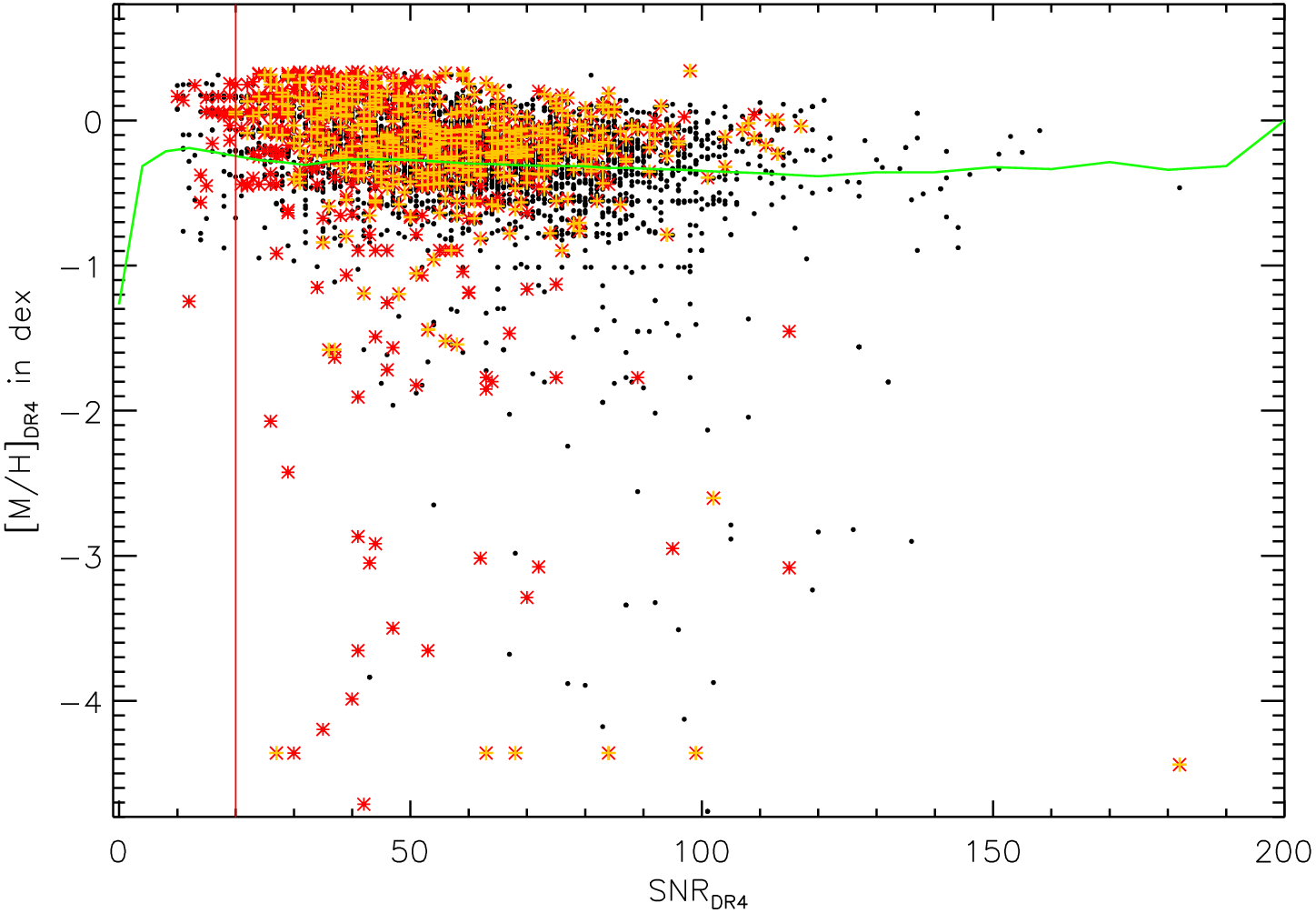
Figure 13: $[M/H]$ distribution with respect to SNR for our high-quality RV sample (black dots). Red asterisks and orange crosses illustrate our good RV and $[M/H]$ members, respectively. The red and green solid lines visualise our adapted cut at an SNR $\geq$ 20 and the overall trend for the entire RAVE DR4, respectively.

Moreover, we examined the $[M/H]$ distribution with respect to $R$ (Fig. 14) and computed the overall trend in RAVE DR4 as $\overline{[M/H]}$ in bins of 4 along $R$. This overall trend indicates a slight correlation of $[M/H]$ with $R$, suggesting that the fewer lines in metal-poor stars lead to a better match of the observed to the template spectrum, at least for stars with $[M/H]\geq-1$ dex. Because of this slope we cannot use the overall trend to evaluate the cut refinement in $R$. However, for $R\leq$ 20 a non-negligible number of good RV members show unexpectedly low $[M/H]$, and we chose the corresponding cut to $R\geq$ 20 for our metallicity study in Galactic open clusters.
We were unable to identify any dependencies of $[M/H]$ on corr_RV and saw no need for additional changes of the constraints for our high-quality $[M/H]$ sample. Combined with the membership probabilities ($P_{kin}$ and $P_{phot}\geq$ 14% or $P_{kin}$ and $P_{phot}\geq$ 61%), the new cuts define our good and best $[M/H]$ members, respectively. In Tab. 6 we summarise the corresponding numbers of measurements, stars, and clusters for our metallicity study.

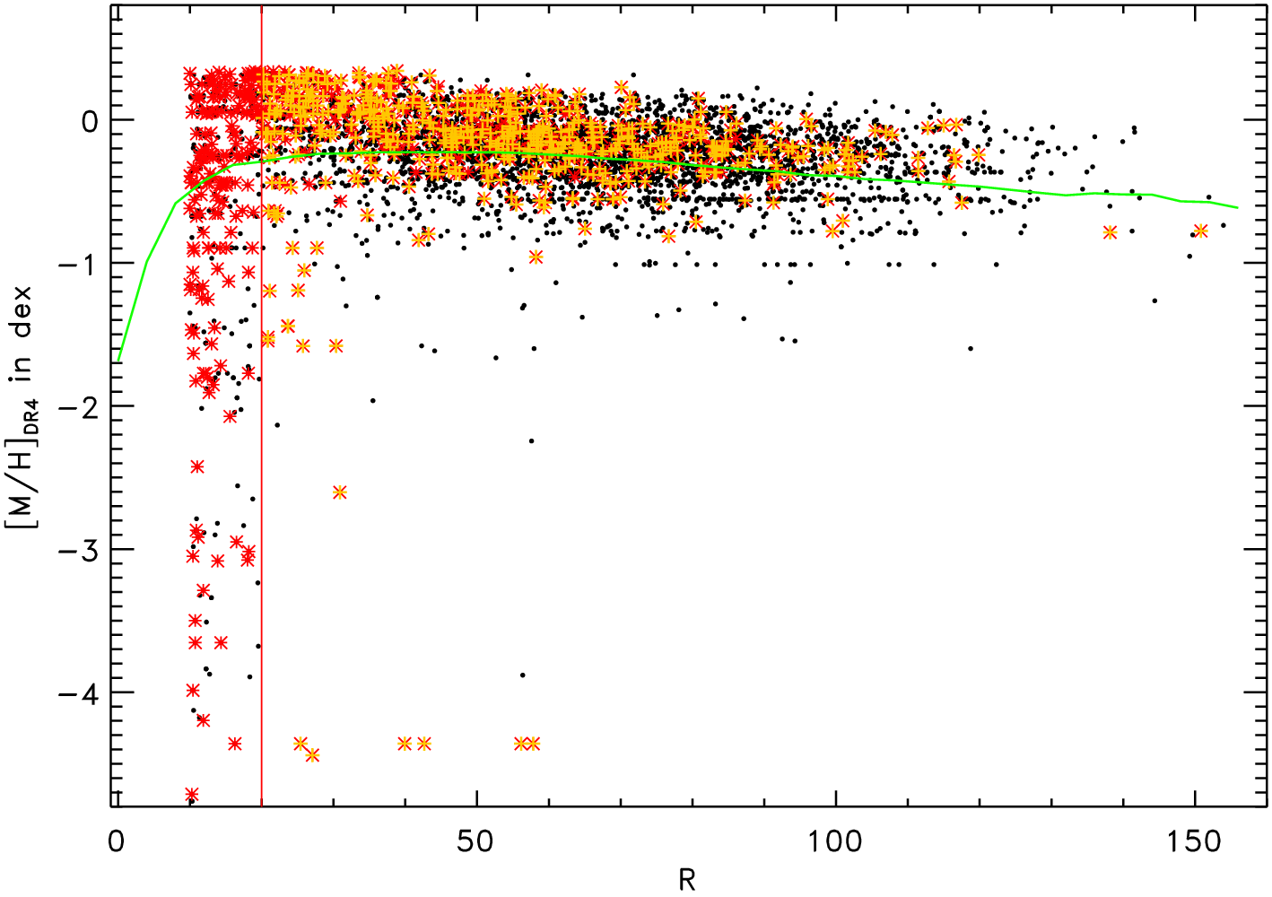
Figure 14: $[M/H]$ distribution with respect to $R$. The symbol color-coding is the same as in Fig 13. The red and green solid lines visualise our adapted cut at $R\geq$ 20 and the overall trend for the entire RAVE DR4, respectively.

Furthermore, we investigated a potential magnitude dependence of $[M/H]$, which might affect the reliability of our data (see Fig. 15). The few members at $[M/H]=-$4.36 dex show obviously unrealistic values and were therefore not considered any further in our metallicity study of OCs. To identify a possible dependence more clearly, we computed the unweighted $\overline{[M/H]}$ and $\sigma[M/H]$ of our high-quality $[M/H]$ sample in bins of 0.5 mag along $V_{Johnson}$. Both show a very flat behaviour and the variations at brighter magnitudes are most likely due to small number statistics and are not representative for the overall trend. Hence, we were unable to identify any considerable magnitude dependence of metallicities in RAVE, confirming our sample to provide reliable results.

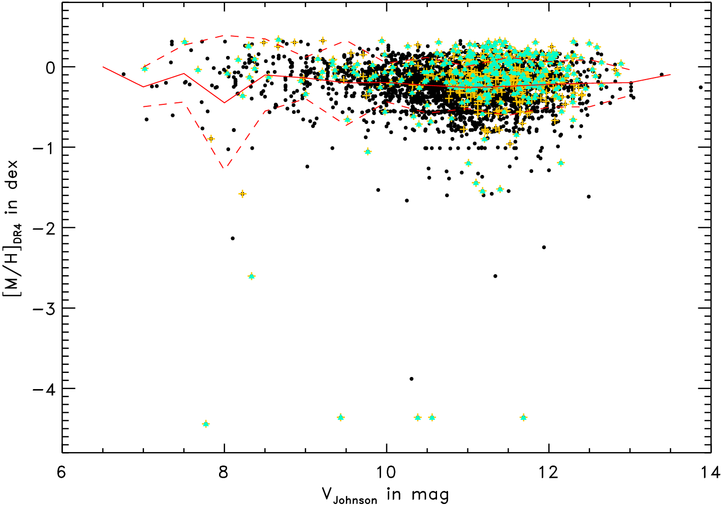
Figure 15: $[M/H]$ distribution with respect to $V_{Johnson}$ for our high-quality $[M/H]$ sample (black dots). Orange crosses and turquoise triangles illustrate good and best $[M/H]$ members, respectively. Red solid and dashed lines visualise $\overline{[M/H]}$ and $\sigma[M/H]$ for our high-quality $[M/H]$ sample, respectively.

Since CSOCA does not provide any metallicity data, no reference values for individual cluster members were available. For cluster mean metallicities, on the other hand, we found reference values in DAML, which we discuss in more detail in Sect. 4.3.

Table 6: Numbers for our different $[M/H]$ samples in RAVE and OC areas.

	RAVE DR4		OC sample
Number of	entire	high-quality	$[M/H]$	high-quality	good $[M/H]$	best $[M/H]$
	RAVE	in RAVE	sample	$[M/H]$ sample	members	members
Measurements	451474	354906	6209	3947	517	308
Stars	405176	322843	4785	3485	455	265
Clusters	—	—	244	192	94	77

4 Mean values for our Galactic open clusters

4.1 Radial velocity

First of all, we cleaned each OC from outliers by applying a $3\sigma$-clipping algorithm to obtain the most representative $\overline{RV}$. Then we determined $\overline{RV}$ for in total 110 OCs and summarise the results in Tab. LABEL:tab1 along with catalogue identifiers, that is, COCD number (Seq) and Name. In addition, we provide two kinds of reference values. On the one hand, we computed $\overline{RV}$ in CRVAD-2, and on the other hand we list values from CRVOCA (Kharchenko et al. 2007). We prefer to use their computed $\overline{RV}$ and only where no calculated $\overline{RV}$ were available we give literature values. For 37 OCs we provide $\overline{RV}$ for the first time.

$$\overline{RV} = \frac{\sum\limits_{i}RV_{i}\cdot g_{i}}{\sum\limits_{i}g_{i}}$$ (1)

$$\sigma\overline{RV} = \sqrt{\frac{n}{n-1}\cdot\frac{\sum\limits_{i}g_{i}\cdot(RV_{i}-\overline{RV})^{2}}{\sum\limits_{i}g_{i}}}$$ (2)

$$\textrm{e}{\overline{RV}} = \frac{\sigma\overline{RV}}{\sqrt{n}}$$ (3)

$$\overline{eRV^{*}} = \frac{\sum\limits_{i}eRV^{*}_{i}\cdot(P_{kin,i}\cdot P_{phot,i})}{\sum\limits_{i}(P_{kin,i}\cdot P_{phot,i})},$$ (4)

with the weights $$g_{i}$$ defined as

$$g_{i} = \frac{P_{kin,i}\cdot P_{phot,i}}{(eRV^{*}_{i})^{2}}.$$ (5)

The $\overline{RV}$ from RAVE and CRVAD-2 were primarily derived from best RV or 1$\sigma$-members, respectively. Only where just one or no most probable member was available we included good RV or 2$\sigma$-members as well to compute the $\overline{RV}$ in RAVE and CRVAD-2, respectively. The corresponding numbers are also included in Tab. LABEL:tab1. CRVOCA includes $\overline{RV}$ based on 3$\sigma$-members, while the $\overline{RV}$ references computed in this work consider at worst 2$\sigma$-members to reduce the field star contamination. A comparison between the reference catalogues yielded a very good agreement, as expected, indicating that in CRVOCA as well the field star contamination can be considered to be relatively low and the values as suitable references.
The provided $\overline{RV}$ in RAVE and CRVAD-2 were calculated as weighted mean considering individual $eRV^{*}$ and membership probabilities $P_{kin}$ and $P_{phot}$ (Eq. 1). As mentioned above, we considered all $eRV^{*}<1$ km/s to be too optimistic and replaced them with 1 km/s, which is also reflected in Tab. LABEL:tab1. We also give typical RV uncertainties in OCs ($\overline{eRV^{*}}$), computed as weighted mean from the individual $eRV^{*}$ of the members (Eq. 4), including only OC membership probabilities as weights. The weighted standard deviation ($\sigma\overline{RV}$; Eq. 2) and uncertainty of $\overline{RV}$ (e$\overline{RV}$; Eq. 3) could only be computed for OCs with at least two individual measurements. For clusters with only one representative we do not provide $\sigma\overline{RV}$ and assume $\overline{eRV^{*}}=eRV^{*}$.

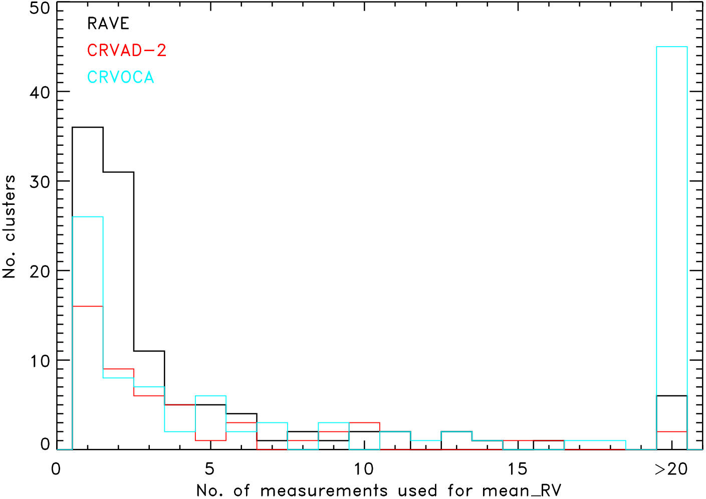
Figure 16: Histogram for the number of measurements or stars used to derive $\overline{RV}$ in RAVE (black) and CRVAD-2 (red), respectively. The cyan histogram shows the number histogram for CRVOCA.

In Fig.16 we show the histograms for the total number of measurements and stars used to obtain the RAVE based and reference $\overline{RV}$, respectively. We only included OCs observed in RAVE. The vast majority of $\overline{RV}$ in all catalogues are based on fewer than six individual RV measurements and only a few OCs show $\overline{RV}$ derived from more than 20 individual RV measurements in either data set. CRVOCA shows the largest number of OCs with more than 20 individual RV values, since they used stars with lower membership probability than we did. Considering the different numbers of OCs covered by the catalogues, the distributions for the number of individual measurements show a very similar shape. This indicates that the resulting $\overline{RV}$ are of similar quality, as expected.

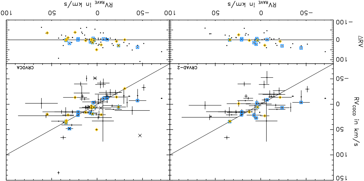
Figure 17: Upper panels: $\overline{RV}$ comparison between RAVE and reference values from CRVAD-2 (left) and CRVOCA (right). The black line shows the one-to-one relations. Lower panels: Corresponding difference distributions with the zero-difference lines included as black solid lines. Blue squares and yellow diamonds illustrate clusters with $\geq$ 10 individual RVs in RAVE and the reference catalogue, respectively. Black crosses indicate missing e$\overline{RV}$ information in CRVOCA.

Fig. 17 illustrates a visual comparison between our RAVE results and available references. The error bars represent the e$\overline{RV}$ in each catalogue. The RV difference ($\Delta\overline{RV}$) is defined as $\Delta\overline{RV}=\overline{RV_{Ref}}-\overline{RV_{RAVE}}$, where $\overline{RV_{Ref}}$ are the reference values obtained from CRVAD-2 or CRVOCA for the corresponding panel. The differences between RAVE results and reference values for our OCs (Fig. 17) appear to be larger than for the individual stars (Fig. 10). One can see a negative slope in the difference distribution, which is mainly caused by two OCs with very large differences and cannot be verified to be statistically significant. Contributing factors to the apparently larger RV differences are the different OC members targeted by either survey and the potential systematics induced by the reference values from Barbier-Brossat & Figon (2000). In general, cluster $\overline{RVs}$ derived from only up to five individual measurements have to be considered with caution in all data sets used in the presented project, that is, RAVE, CRVAD-2, and CRVOCA.
OCs with more than ten individual measurements in RAVE, on the other hand, show a very good agreement, except for three. The three exceptions (Platais 8, Sco-OB 4, and Sgr-OB 7; left panel of Fig. 17) are all associations, which naturally show an intrinsically higher velocity dispersion, because they are not as tightly bound as open clusters. Since the membership selection is partly based on kinematics, it might be possible that for associations as well mistaken membership can contribute to the larger differences, in particular because different objects were targeted by RAVE and CRVAD-2. CRVAD-2 references with more than ten individual RV measurements also show a good agreement, except for two actual open clusters: NGC 2516 and Collinder 228. In CRVOCA even better measured OCs show relatively large differences to the RAVE results. Thus, the field star contamination in CRVOCA is not negligible, though we stated it to be relatively low. Furthermore, we can conclude that RAVE provides more reliable $\overline{RV}$ than CRVAD-2.

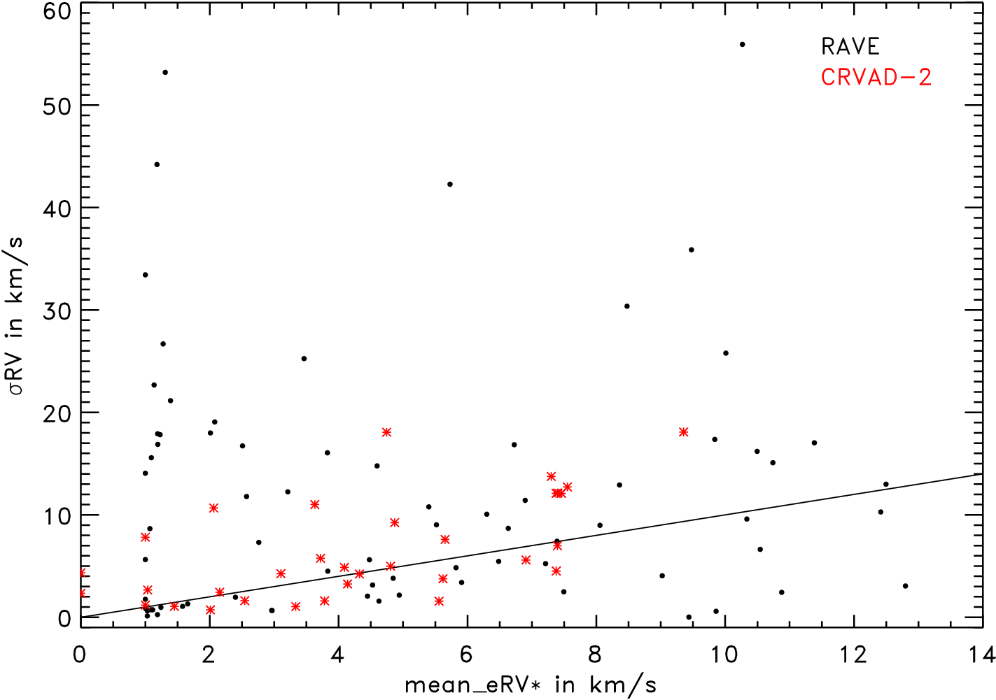
Figure 18: Comparison of $\sigma\overline{RV}$ to $\overline{eRV^{*}}$ in CRVAD-2 (red asterisks) and RAVE (black dots) for OCs observed by RAVE. The black solid line represents the one-to-one relation.

In addition, we compared $\sigma\overline{RV}$ and $\overline{eRV^{*}}$ in RAVE and CRVAD-2 (Fig. 18). In both catalogues only very few OCs show $\sigma\overline{RV}$ similar to $\overline{eRV^{*}}$, the majority show higher $\sigma\overline{RV}$, and in certain cases they are about a factor of 5-10 higher than $\overline{eRV^{*}}$. There are several possible reasons, namely small number statistics, partly mistaken membership, or undetected binarity. Due to the first aspect, the $\sigma\overline{RV}$ have to be considered with care and cannot be regarded in any way representative for the internal cluster velocity dispersion. The aspect of binarity in our OCs is discussed in Sect. 4.2. Partly mistaken membership might be minimised when updated membership probabilities from the Milky Way Star Cluster (MWSC) survey (Kharchenko et al. 2012) become available.
Moreover, it would be a great improvement to also include RVs as criteria for OC membership, but this is only reasonable when RV data are available for all stars in OC areas. The CRVAD-2 $\sigma\overline{RV}$ are well below 20 km/s, whereas the RAVE values reach up to 60 km/s. Most likely, this is due to the different targets included to compute $\overline{RV}$ for the two catalogues (see Sect. 3.2).

4.2 Binarity fraction

Above we pointed out that undetected binaries can have a significant influence on the accuracy of our $\overline{RV}$ results. For a detailed study multiple epochs for each member would be needed. We examined our best RV members in RAVE for multiple epochs and only identified 76 out of 443 stars, where each object is only provided with two measurements. This is by far not enough for a deep binary study based on RAVE data. Hence, we have to work with limited sources of information to give an approximate idea on the binary fraction in our sample.
In a first step we checked the duplicity flags in CSOCA and found 14 stars indicated as potential or confirmed binaries among our 443 best RV members. Secondly, we cross-matched our best RV members with the list of SB1 (Matijevič et al. 2011) and SB2 (Matijevič et al. 2010) binaries in RAVE and found no common object. This is not surprising, since we rejected objects with bad spectral flags from Matijevič et al. (2012). If we only consider the cuts SNR $\geq$ 10, $R\geq$ 10, and $|corr\_RV|\leq$ 9 km/s in RAVE along with $P_{kin}$ and $P_{phot}\geq$ 61%, we find 11 SB2 binaries in 4 OCs. However, all these numbers are far below the 6% binary fraction suggested by Matijevič et al. (2011).
Moreover, we provide a rough estimate on the binary fraction based on RAVE data using a very simple approach, namely that the large scatter in Fig. 17 and the high $\sigma\overline{RV}$ are mainly caused by undetected binarity. For each cluster we first computed the difference between individual RVs and $\overline{RV}$. Then we compared these differences with 3$\overline{eRV^{*}}$, defining our assumed velocity dispersion. This analysis can only be made for OCs with at least two individual measurements, which reduces the number of clusters considered to 76. We assumed members exceeding the 3$\overline{eRV^{*}}$ limit to be potential binaries and calculated the binary fraction with respect to the total number of RAVE measurements in the corresponding OC. The results are summarised in Tab. 7.

Table 7: Results for our rough binary fraction estimate in OCs with at least two RV measurements in RAVE.

binary fraction	0%	$\leq$25%	25-50%	$\geq$50%	total
No. of OCs	41	9	7	17	74
Proportion (%)	55.4	12.2	9.5	23.0	—

About half of our OCs with at least two RV measurements show no binarity and another 23% show a very high estimated binary fraction ($\geq$50%). This effect is most likely due to small number statistics, where the binary fraction can change fast from 0% to more than 50% if just one more star is outside the defined 3$\overline{eRV^{*}}$ limit. Therefore, the listed numbers can at most be considered as lower limits. In Tab. LABEL:tab1 about 45.9% of OCs with at least two RV measurements show $\sigma\overline{RV}\geq 10$ km/s, which is similar to the 44.7% of OCs with non-zero binary fraction. This verifies that undetected binaries are a dominant effect that induces unexpectedly high $\sigma\overline{RV}$ for our OCs.

4.3 Metallicity

Because of the more stringent requirements in our $[M/H]$ study, we were able to determine $\overline{[M/H]}$ for only 81 of our 110 OCs with $\overline{RV}$ in RAVE. Because we strictly distinguished between iron abundances and overall metallicities in DAML (see Sect. 2.3), we obtained reference $\overline{[M/H]}$ for only 12 OCs. Hence, for 69 clusters we present $\overline{[M/H]}$ for the first time. The results are summarised in Tab. LABEL:tab2 along with the cluster identifiers (COCD number and cluster name). Our metallicity results were primarily obtained from best $[M/H]$ member measurements after cleaning each OC from outliers by applying a 3$\sigma$-clipping algorithm. Only where no or just one best $[M/H]$ member measurement was available we included good $[M/H]$ member measurements as well. The number of best and additional good $[M/H]$ member measurements are also included in Tab. LABEL:tab2. We computed the $\overline{[M/H]}$ as weighted mean with respect to the membership probabilities (Eq. 6), since the listed $e[M/H]^{*}$ show a very discrete distribution and might not reflect realistic measurements errors (see Sect. 3.3). For OCs with at least two individual $[M/H]$ measurements we computed weighted standard deviations ($\sigma\overline{[M/H]}$; Eq. 7) and uncertainties of $\overline{[M/H]}$ (e$\overline{[M/H]}$; Eq. 8).

$$\overline{[M/H]} = \frac{\sum\limits_{i}[M/H]_{i}\cdot w_{i}}{\sum\limits_{i}w_{i}}$$ (6)

$$\sigma\overline{[M/H]} = \sqrt{\frac{n}{n-1}\cdot\frac{\sum\limits_{i}w_{i}\cdot([M/H]_{i}-\overline{[M/H]})^{2}}{\sum\limits_{i}w_{i}}}$$ (7)

$$\textrm{e}{\overline{[M/H]}} = \frac{\sigma\overline{[M/H]}}{\sqrt{n}},$$ (8)

with the weights $$w_{i}$$ defined as

$$w_{i} = P_{kin,i}\cdot P_{phot,i}.$$ (9)

In Fig. 19 we display the histograms for the number of measurements and stars used to obtain $\overline{[M/H]}$ in RAVE and DAML, respectively. Again we only included OCs with $[M/H]$ data available in RAVE. As expected, the vast majority of OCs are covered by fewer than six individual $[M/H]$ measurements and small number statistics might affect our results. The number of references is too small to conclude about the shape of the number distribution.

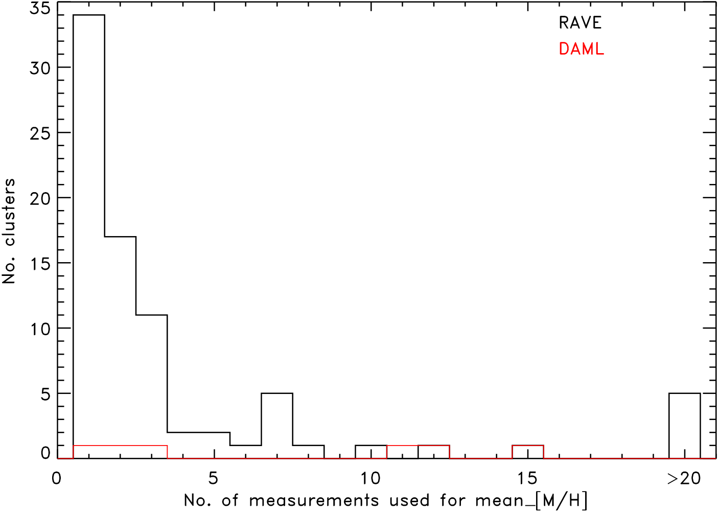
Figure 19: Histogram for the number of measurements or stars used to obtain $\overline{[M/H]}$ in RAVE (black) and DAML (red), respectively.

From Fig. 20 one can see that the majority of OCs in RAVE, except for four, agree very well with the values from DAML within the uncertainties. We define the differences between the catalogues as $\Delta\overline{[M/H]}=\overline{[M/H]_{DAML}}-\overline{[M/H]_{RAVE}}$ and they appear to be similar to the uncertainties. Only the Pleiades (Melotte 22) are covered by more than ten individual measurements in RAVE and agree very well. In addition to the Pleiades, DAML lists two more clusters with $\overline{[M/H]}$ based on more than ten values, namely NGC 2422 and NGC 2354.
Our metallicity study in RAVE can only give a rough idea on the $[M/H]$ behaviour of the Galactic OC system. The typical uncertainties of $\overline{[M/H]}$ and individual members, obtained from the pipeline, are about 0.1 dex and reflect only internal errors. When including external errors as well, the typical errors are about 0.3 dex (Boeche et al. 2011). The RAVE $[M/H]$ accuracy is apparently not high enough to carry out a detailed metallicity study within OCs.

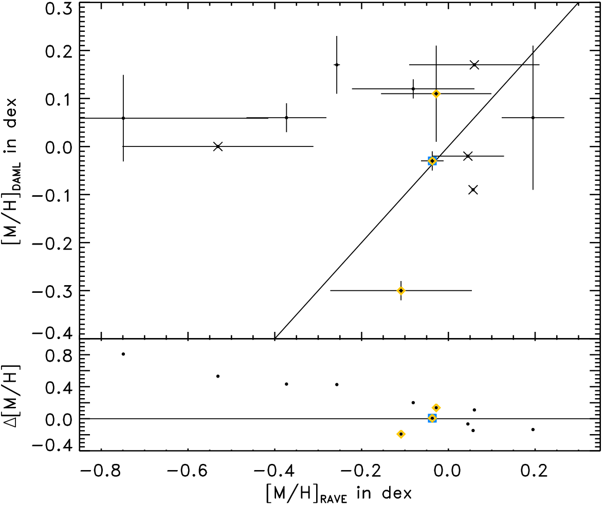
Figure 20: $\overline{[M/H]}$ comparison (upper panel) and difference distribution (lower panel) between RAVE DR4 and DAML, along with the one-to-one relation and zero-difference line (black solid lines). Blue squares and yellow diamonds highlight OCs with $\geq$10 individual $[M/H]$ measurements in RAVE DR4 and DAML, respectively. Black crosses indicate e$\overline{[M/H]}$ missing in one or both catalogues.

A brief look at the difference distribution might suggest a negative slope with increasing metallicities. This apparent slope is primarily caused by four clusters, which are metal poor in RAVE. If we eliminate them, the distribution is consistent with not showing any trend and is centred around zero. In Tab. LABEL:tab2 we found ten clusters and associations with $\overline{[M/H]}$ below $-0.5$ dex. This contradicts our expectation that open clusters and associations in the solar neighbourhood have about solar metallicity. Except for one OC with three best $[M/H]$ member measurements, the $\overline{[M/H]}$ values for all metal-poor OCs are based on either one best $[M/H]$ member or mainly on good $[M/H]$ members. Therefore, mistaken membership in combination with small number statistics can be one reason for very low $\overline{[M/H]}$.
However, this would not explain the amount of very metal poor OCs we found in our sample, since our membership selection used a uniform algorithm on homogeneous spatial, photometric, and kinematic information. These unexpectedly metal-poor OCs could also indicate that the RAVE DR4 pipeline might underestimate the corresponding metallicities for certain spectra. This is supported by our finding that three out of the 23 individual $[M/H]$ measurements of Pleiades best members show values of $-4.36$ dex, which we excluded when we computed $\overline{[M/H]}$.
To verify this hypothesis we analysed the results of the chemical pipeline implemented for RAVE by Boeche et al. (2011). These authors employed slightly more stringent quality constraints (SNR $\geq 20$, $v_{rot}<50$ km/s and $4000<T_{eff}<7000$ K). It also has to be noted that the chemical pipeline does not cover the very metal-poor end, which the DR4 pipeline does, since either the data quality is too low or the spectral characteristics are not covered by the data grid used in the chemical pipeline. Hence, the chemical pipeline provides $\overline{[M/H]}$ for only 52 OCs with typically fewer individual measurements after applying our quality requirements on this data set. We included these additional results in Tab. LABEL:tab2 along with the number of good and best member measurements in this data set and show a comparison to our reference $\overline{[M/H]}$ in Fig. 21.

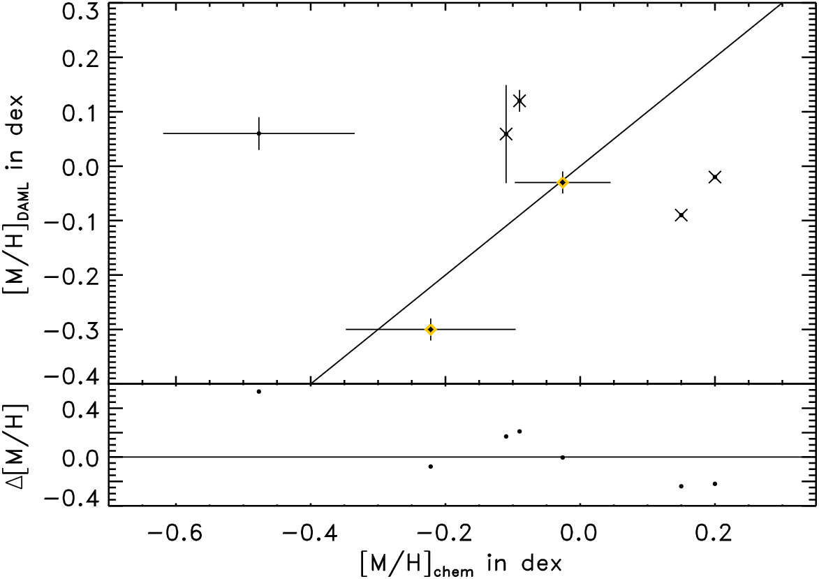
Figure 21: $\overline{[M/H]}$ comparison (upper panel) and difference distribution (lower panel) between the results from the RAVE chemical pipeline (Boeche et al. 2011) and DAML, along with the one-to-one relation and zero-difference line (black solid lines). Yellow diamonds highlight OCs with $\geq$10 individual $[M/H]$ measurements in DAML. Black crosses indicate e$\overline{[M/H]}$ missing in one or both catalogues.

The two RAVE metallicity sets, DR4 and the chemical pipeline, agree well with the references from DAML in the range $-0.5<\overline{[M/H]}<0.5$. However, the chemical pipeline does not provide any very metal-poor values for targets that match our quality requirements, and such stars are simply not listed in the resulting data table. This might indicate that the apparently very metal poor stars in DR4 suffer from lower data quality. Future investigation will show whether all these very metal-poor OCs simply arise from mistaken membership combined with low number statistics or if potentially underestimated metallicities in RAVE DR4 might also play a role.

5 Summary and discussion

Current compilations and catalogues of Galactic open clusters significantly lack spectroscopic information, such as RVs and abundances. The RAVE survey allows us to fill in some of the missing data. Our project is based on the most homogeneous OC catalogue by Kharchenko et al. (2005a, b) (COCD) and the corresponding stellar catalogue (CSOCA).
Via a cross-match we identified OC members in RAVE DR4, with a bias towards fainter stars. For the cleaned working sample we provided new RV and $[M/H]$ data. Interestingly, our OC members in RAVE do not represent the accuracy of the entire survey. We showed that this is most likely due to the higher percentage of dwarfs in our OC sample. Still, the data quality is sufficient for determining $\overline{RV}$ and $\overline{[M/H]}$ for Galactic open clusters, since the selected members agree well with previous RV data in OCs.
We were able to derive $\overline{RV}$ for 110 OCs, including new data for 37 open clusters. $\overline{[M/H]}$ we derived for only 81 OCs, due to more stringent constraints for our metallicity sample. For 69 of these OCs we presented metallicities for the first time. The $\overline{RV}$ sample agrees better with the reference values than the $\overline{[M/H]}$ based on RAVE DR4. The relatively large spread in both comparison distributions is most likely caused by different stellar samples for each OC in RAVE and the reference catalogue, partly mistaken OC membership, or undetected binarity. Partly mistaken membership may be minimised when the updated membership probabilities from the Milky Way Star Cluster (MWSC) survey (Kharchenko et al. 2012) become available. Furthermore, most of our results are based on only a few individual measurements, which in general makes them less robust against the effects mentioned. All these clusters in RAVE and the reference catalogues have to be considered with caution.
Studies by Kouwenhoven & de Grijs (2008), Geller et al. (2008, 2010), and Gieles et al. (2010) also indicate that binarity may significantly affect the internal velocity dispersion of open clusters. Although we cannot consider our $\sigma\overline{RV}$ to be representative for the internal cluster velocity dispersion, we come to the same conclusion based on a rough estimate on binarity in the considered OCs, yielding a similar number of OCs with potential binaries present and OCs with unusually high $\sigma\overline{RV}$.
Our $\sigma\overline{RV}$ results are of sufficient quality to derive reliable 3D-kinematics for the Galactic OC system. Combined with previous RV data on OCs this enabled us to re-evaluate the open cluster groups and complexes, proposed by Piskunov et al. (2006). The additional abundance data obtained by RAVE may only give us a rough idea on the $[M/H]$ behaviour of the Galactic OC system. We found ten OCs with $\overline{[M/H]}<-0.5$ dex, which are too metal poor considering that they are located in the solar neighbourhood. Hence, the DR4 metallicities presented in this work have to be considered with care.
Based on inter-cluster differences we can draw conclusions on potential formation scenarios of the re-investigated open cluster groupings. For a very detailed picture high-resolution results would be necessary, which was previously suggested by Carrera et al. (2007) and Carrera (2012). In a second paper (Conrad et al. in prep.) we will present more results of our ongoing project on the OC groups and complexes.

Tab. LABEL:tab1. Results from our radial velocity study on open clusters in RAVE, along with reference values from CRVAD-2 and CRVOCA (see Sect. 4.1).
		RAVE					CRVAD-2					CRVOCA
Seq	Name	$\overline{RV}$	e$\overline{RV}$	$\sigma\overline{RV}$	$\overline{eRV^{*}}$	No. of	$\overline{RV}$	e$\overline{RV}$	$\sigma\overline{RV}$	$\overline{eRV^{*}}$	No. of	$\overline{RV}$	e$\overline{RV}$	No. of
		km/s	km/s	km/s	km/s	entriesa	km/s	km/s	km/s	km/s	entriesa	km/s	km/s	starsb
3	Blanco 1	6.168	6.737	17.825	1.229	7 (  –)	2.843	1.761	4.981	4.807	8 (  –)	3.580	2.360	13
44	Alessi 13	1.053	0.458	0.647	2.967	2 (  –)	15.916	1.353	2.344	0.000	1 (  2)	19.530	3.000	3
47	Melotte 22	3.503	0.391	1.955	2.399	25 (  –)	5.766	0.241	1.616	2.543	45 (  –)	5.900	0.450	106
65	NGC 1901	-1.354	0.478	0.676	2.962	2 (  –)	—	—	—	—	– (  –)	-9.630	9.630	3
77	Collinder 70	54.817	1.000	—	1.000	1 (  –)	24.038	1.917	5.750	3.719	9 (  –)	19.870	2.190	23
127	NGC 2354	42.320	8.117	14.060	1.000	3 (  –)	—	—	—	—	– (  –)	33.400	0.270	6
129	Alessi 3	-2.143	0.531	1.302	1.658	1 (  5)	—	—	—	—	– (  –)	20.000	7.400	-1
133	Collinder 135	26.957	10.140	22.673	1.136	5 (  –)	16.173	0.782	1.564	5.558	4 (  –)	15.350	2.200	4
142	Bochum 5	27.881	11.293	25.251	3.464	5 (  –)	—	—	—	—	– (  –)	41.000	2.000	1
147	NGC 2422	34.212	0.872	3.145	4.527	13 (  –)	34.408	1.862	5.587	6.908	9 (  –)	36.720	2.920	13
148	NGC 2423	21.069	2.041	12.244	3.211	36 (  –)	20.913	3.190	7.813	1.000	6 (  –)	21.670	2.540	9
149	Ruprecht 26	39.079	7.765	17.362	9.839	5 (  –)	15.000	3.700	—	3.700	1 (  –)	15.000	3.700	1
150	Melotte 71	0.545	1.000	—	1.000	1 (  –)	—	—	—	—	– (  –)	50.140	0.140	11
152	NGC 2428	46.665	2.727	5.454	6.484	4 (  –)	—	—	—	—	– (  –)	—	—	–
153	NGC 2430	31.337	11.831	16.732	2.509	2 (  –)	—	—	—	—	– (  –)	—	—	–
158	Ruprecht 151	31.294	4.841	16.056	3.826	11 (  –)	—	—	—	—	– (  –)	—	—	–
159	NGC 2451A	56.185	30.712	53.195	1.309	– (  3)	25.721	5.332	10.664	2.062	4 (  –)	22.630	4.490	9
160	NGC 2437	30.432	4.048	16.194	10.496	16 (  –)	—	—	—	—	– (  –)	48.090	0.000	1
163	NGC 2447	31.959	6.222	10.777	5.400	3 (  –)	20.925	1.088	2.665	1.036	6 (  –)	21.310	0.670	11
164	NGC 2448	27.195	1.245	2.157	4.941	– (  3)	15.000	3.700	—	3.700	1 (  –)	15.000	3.700	1
166	Haffner 16	37.246	3.031	—	3.031	1 (  –)	65.800	3.700	—	3.700	1 (  –)	65.800	3.700	1
167	NGC 2477	6.374	0.184	0.261	1.188	2 (  –)	—	—	—	—	– (  –)	7.320	0.130	49
171	NGC 2482	42.155	0.910	1.577	4.626	3 (  –)	—	—	—	—	– (  –)	—	—	–
175	NGC 2516	-4.492	4.994	8.649	1.071	– (  3)	22.937	0.330	1.043	3.334	10 (  –)	20.670	1.450	23
180	NGC 2527	42.425	1.268	3.803	4.846	9 (  –)	—	—	—	—	– (  –)	135.100	3.000	-1
182	Vel OB2	20.840	3.598	16.878	1.193	– (22)	15.163	5.370	7.594	5.652	2 (  –)	15.450	3.200	6
191	Haffner 26	62.377	12.076	—	12.076	1 (  –)	—	—	—	—	– (  –)	—	—	–
192	NGC 2567	37.020	1.000	—	1.000	1 (  –)	—	—	—	—	– (  –)	35.790	0.090	1
193	NGC 2571	44.021	10.280	—	10.280	1 (  –)	—	—	—	—	– (  –)	—	—	–
201	NGC 2632	34.001	0.285	1.065	1.578	14 (  –)	34.117	0.425	2.442	2.154	33 (  –)	33.660	1.180	73
202	IC 2391	12.487	3.533	—	3.533	1 (  –)	15.318	1.336	4.225	4.323	10 (  –)	16.040	2.530	18
212	NGC 2682	33.806	0.301	0.852	1.004	8 (  –)	33.555	0.307	1.190	1.000	15 (  –)	32.300	1.100	33
216	Platais 8	7.349	8.046	26.687	1.276	11 (  –)	21.495	4.935	6.980	7.396	2 (  –)	17.320	3.090	5
223	Turner 5	-1.195	14.952	21.145	1.391	2 (  –)	—	—	—	—	– (  –)	26.200	3.700	-1
226	Ruprecht 80	45.749	1.000	—	1.000	1 (  –)	—	—	—	—	– (  –)	—	—	–
230	NGC 3036	11.777	1.000	—	1.000	1 (  –)	—	—	—	—	– (  –)	—	—	–
243	IC 2581	2.165	14.146	—	14.146	1 (  –)	-0.658	0.510	0.721	2.010	2 (  –)	-4.640	3.510	5
248	Collinder 223	8.553	0.087	0.124	1.031	2 (  –)	—	—	—	—	– (  –)	4.700	0.000	1
249	Ruprecht 90	18.079	7.269	10.280	12.415	2 (  –)	-40.000	4.400	—	4.400	1 (  –)	-40.000	4.400	1
251	Loden 153	13.698	5.247	7.420	7.390	2 (  –)	-11.824	2.502	4.334	0.000	1 (  2)	-10.330	2.400	3
254	NGC 3324	-4.042	2.864	4.051	9.023	2 (  –)	-8.500	3.700	—	3.700	1 (  –)	-8.500	4.200	1
255	vdBergh 99	12.790	3.684	9.025	5.518	6 (  –)	11.340	0.751	1.062	1.450	2 (  –)	6.000	3.490	4
258	Melotte 101	20.265	10.383	—	10.383	1 (  –)	—	—	—	—	– (  –)	—	—	–
259	IC 2602	5.042	2.365	19.066	2.077	65 (  –)	27.163	2.127	4.255	3.104	4 (  –)	19.020	2.930	12
260	Bochum 10	-1.485	4.592	—	4.592	1 (  –)	-2.300	1.800	—	1.800	1 (  –)	-2.300	1.800	1
261	Alessi 5	6.339	3.183	4.501	3.832	2 (  –)	10.867	8.585	12.141	7.400	2 (  –)	12.800	8.800	2
262	Collinder 228	24.240	13.119	—	13.119	1 (  –)	-1.161	5.712	18.062	4.746	10 (  –)	-13.460	3.270	24
266	Ruprecht 91	-4.115	11.325	—	11.325	1 (  –)	—	—	—	—	– (  –)	7.300	0.000	1
267	Loden 189	10.493	4.499	10.060	6.300	5 (  –)	—	—	—	—	– (  –)	—	—	–
268	Ruprecht 92	-10.582	3.703	5.237	7.212	2 (  –)	—	—	—	—	– (  –)	-15.600	1.800	-1
270	Trumpler 17	25.506	1.719	2.431	10.877	2 (  –)	—	—	—	—	– (  –)	—	—	–
271	Collinder 236	14.140	11.531	25.785	10.011	5 (  –)	—	—	—	—	– (  –)	—	—	–
273	NGC 3496	2.321	1.962	3.398	5.909	1 (  2)	—	—	—	—	– (  –)	-51.400	0.000	1
274	Pismis 17	-47.146	0.517	0.731	1.086	2 (  –)	—	—	—	—	– (  –)	61.700	0.000	1
275	Ruprecht 93	5.072	3.502	—	3.502	1 (  –)	—	—	—	—	– (  –)	—	—	–
276	NGC 3532	4.311	0.572	2.061	4.448	13 (  –)	-2.252	6.355	11.008	3.630	3 (  –)	-3.040	3.810	5
283	Trumpler 18	-10.016	12.474	—	12.474	1 (  –)	-20.000	7.400	—	7.400	1 (  –)	-20.000	7.400	1
287	NGC 3680	2.154	1.000	—	1.000	1 (  –)	—	—	—	—	– (  –)	8.000	3.670	7
298	Loden 481	16.915	8.672	—	8.672	1 (  –)	-7.100	1.200	—	1.200	1 (  –)	-22.050	14.950	2
304	ESO 130-06	-1.227	3.424	4.842	5.822	2 (  –)	—	—	—	—	– (  –)	—	—	–
305	Loden 565	-17.872	9.328	—	9.328	1 (  –)	10.100	1.000	—	1.000	1 (  –)	10.100	0.200	1
306	ESO 130-08	-38.522	6.346	8.974	8.057	2 (  –)	—	—	—	—	– (  –)	—	—	–
309	NGC 4349	-11.929	3.239	5.611	4.478	3 (  –)	-15.700	1.800	—	1.800	1 (  –)	-15.690	1.780	1
310	Collinder 258	-14.349	9.186	12.992	12.496	2 (  –)	—	—	—	—	– (  –)	—	—	–
322	Stock 16	-6.875	6.780	9.589	10.336	2 (  –)	-52.787	12.634	21.883	37.024	3 (  –)	-41.800	8.790	5
324	Loden 821	-3.718	5.705	11.410	6.896	4 (  –)	-39.000	7.400	—	7.400	1 (  –)	-39.000	7.400	1
327	Basel 18	-21.989	3.021	—	3.021	1 (  –)	—	—	—	—	– (  –)	—	—	–
328	Hogg 16	-51.341	2.159	3.053	12.798	2 (  –)	-29.793	6.047	12.093	7.460	4 (  –)	-33.000	6.160	5
333	Loden 915	-21.605	11.760	—	11.760	1 (  –)	—	—	—	—	– (  –)	—	—	–
335	Loden 1010	-18.238	3.313	6.627	10.544	4 (  –)	—	—	—	—	– (  –)	—	—	–
336	NGC 5281	-15.912	13.073	—	13.073	1 (  –)	—	—	—	—	– (  –)	—	—	–
337	Platais 12	-11.048	2.228	14.777	4.597	44 (  –)	—	—	—	—	– (  –)	-11.990	9.510	2
338	NGC 5316	9.983	5.271	12.911	8.360	6 (  –)	—	—	—	—	– (  –)	—	—	–
339	Loden 995	-6.064	1.224	—	1.224	1 (  –)	—	—	—	—	– (  –)	—	—	–
343	Ruprecht 110	-36.646	3.981	5.631	1.000	2 (  –)	—	—	—	—	– (  –)	—	—	–
356	Alessi 6	19.950	1.000	—	1.000	1 (  –)	—	—	—	—	– (  –)	—	—	–
367	Nor OB5	-20.248	6.805	11.787	2.571	1 (  2)	-26.863	6.048	12.097	7.375	4 (  –)	-23.140	5.110	7
382	NGC 6204	11.580	0.411	0.581	9.859	2 (  –)	—	—	—	—	– (  –)	-51.000	5.800	5
387	NGC 6242	39.324	39.549	55.931	10.268	2 (  –)	—	—	—	—	– (  –)	—	—	–
390	NGC 6250	-16.754	0.010	0.015	9.437	2 (  –)	—	—	—	—	– (  –)	—	—	–
393	Sco OB4	-23.559	8.136	42.275	5.729	27 (  –)	6.853	1.843	4.514	7.378	6 (  –)	5.390	4.950	17
396	vdBergh 221	5.196	5.566	—	5.566	1 (  –)	—	—	—	—	– (  –)	6.330	3.840	3
397	IC 4651	-30.406	0.312	0.624	1.031	4 (  –)	—	—	—	—	– (  –)	-31.000	0.200	14
399	Antalova 1	-6.347	12.041	17.029	11.384	2 (  –)	33.000	40.600	—	40.600	1 (  –)	33.000	40.600	1
402	NGC 6383	-16.537	10.667	15.085	10.740	2 (  –)	1.881	2.659	3.760	5.620	2 (  –)	2.670	2.170	3
403	Trumpler 27	-35.281	1.241	1.755	1.000	2 (  –)	-15.800	1.300	—	1.300	1 (  –)	-15.800	1.300	1
404	Trumpler 28	-32.768	11.912	16.846	6.726	2 (  –)	—	—	—	—	– (  –)	—	—	–
405	ESO 139-13	-33.871	1.000	—	1.000	1 (  –)	—	—	—	—	– (  –)	—	—	–
408	NGC 6405	-7.049	2.746	8.683	6.633	10 (  –)	-8.857	2.295	3.245	4.139	2 (  –)	-11.500	3.500	2
410	Alessi 9	-71.015	1.000	—	1.000	1 (  –)	-11.600	1.200	—	1.200	1 (  –)	-11.600	1.200	1
411	NGC 6416	-11.201	12.724	17.994	2.010	2 (  –)	—	—	—	—	– (  –)	—	—	–
413	NGC 6425	5.439	12.130	—	12.130	1 (  –)	—	—	—	—	– (  –)	—	—	–
418	Sco OB5	-10.453	6.425	—	6.425	1 (  –)	—	—	—	—	– (  –)	—	—	–
420	NGC 6475	-21.377	12.720	—	12.720	1 (  –)	-13.665	0.400	1.600	3.782	16 (  –)	-14.210	1.390	31
429	NGC 6546	-29.427	1.000	—	1.000	1 (  –)	—	—	—	—	– (  –)	-16.670	15.770	3
430	vdBergh 113	16.148	1.755	2.482	7.495	2 (  –)	-16.000	3.700	—	3.700	1 (  –)	-16.000	3.700	1
435	Sgr OB7	-44.478	9.602	30.365	8.477	10 (  –)	-3.576	2.176	4.867	4.091	5 (  –)	-7.190	3.140	9
436	Markarian 38	-33.031	0.515	0.728	1.114	2 (  –)	6.000	9.100	—	9.100	1 (  –)	-3.200	9.200	2
444	NGC 6618	-44.577	0.682	0.965	1.242	2 (  –)	-14.662	12.788	18.085	9.355	2 (  –)	-17.000	13.000	2
445	Trumpler 33	-8.544	7.741	—	7.741	1 (  –)	—	—	—	—	– (  –)	—	—	–
449	IC 4725	61.206	17.938	35.876	9.477	4 (  –)	2.051	7.935	13.745	7.301	3 (  –)	-1.810	10.460	7
452	Ruprecht 145	-8.357	1.000	—	1.000	1 (  –)	—	—	—	—	– (  –)	—	—	–
1033	ASCC 33	34.522	25.521	44.203	1.181	– (  3)	14.692	8.995	12.720	7.551	2 (  –)	15.000	9.000	2
1057	ASCC 57	2.463	7.312	17.911	1.191	6 (  –)	—	—	—	—	– (  –)	—	—	–
1078	ASCC 78	-14.558	5.508	15.578	1.093	8 (  –)	—	—	—	—	– (  –)	—	—	–
1085	ASCC 85	11.160	8.549	—	8.549	1 (  –)	—	—	—	—	– (  –)	7.090	0.000	1
1089	Alessi 24	-38.648	19.301	33.430	1.000	3 (  –)	—	—	—	—	– (  –)	12.300	8.300	2
1091	ASCC 91	-14.513	1.000	—	1.000	1 (  –)	—	—	—	—	– (  –)	—	—	–
1093	ASCC 93	-14.545	12.428	—	12.428	1 (  –)	-19.371	5.334	9.238	4.869	3 (  –)	-23.330	6.360	3
1097	Alessi 40	-16.312	5.168	7.308	2.761	2 (  –)	—	—	—	—	– (  –)	—	—	–
aThe numbers in brackets are the numbers of additional good-member measurements used to compute the $\overline{RV}$.
b “$-1$” indicates clusters where only one star was considered as representative with $P_{kin}>1\%$.

Tab. LABEL:tab2. $\overline{[M/H]}$ for our OCs in RAVE, along with uncertainties, number of individual $[M/H]$ measurements, and reference values from DAML (see Sect. 4.3).
		RAVE DR4					RAVE chem. pipeline			DAML
Seq	Name	$\overline{[M/H]}$	e$\overline{[M/H]}$	$\sigma\overline{[M/H]}$	$\overline{e[M/H]^{*}}$	No. of	$\overline{[M/H]}$	e$\overline{[M/H]}$	No. of	$\overline{[M/H]}$	e$\overline{[M/H]}$	No.	Tech.	Ref.
		dex	dex	dex	dex	entriesa	dex	dex	entriesa	dex	dex	stars
3	Blanco 1	-0.188	0.082	0.216	0.098	7 (  –)	-0.148	0.092	6 (  –)	—	—	–	—	—
44	Alessi 13	0.060	0.150	—	0.150	1 (  –)	—	—	– (  –)	0.170	—	–	CMD	Po10
47	Melotte 22	-0.037	0.026	0.116	0.116	20 (  –)	-0.026	0.071	6 (  –)	-0.030	0.020	15	REC	G00
65	NGC 1901	-0.018	0.092	0.160	0.110	1 (  2)	—	—	– (  –)	—	—	–	—	—
77	Collinder 70	0.144	0.080	—	0.080	1 (  –)	0.150	—	1 (  –)	—	—	–	—	—
127	NGC 2354	-0.109	0.163	0.282	0.094	3 (  –)	-0.222	0.126	3 (  –)	-0.300	0.020	12	DDO	Cl99
129	Alessi 3	-0.275	0.065	0.160	0.111	1 (  5)	-0.387	0.098	– (  5)	—	—	–	—	—
133	Collinder 135	-0.219	0.093	0.209	0.096	5 (  –)	-0.249	0.134	5 (  –)	—	—	–	—	—
142	Bochum 5	-0.171	0.096	0.193	0.105	4 (  –)	-0.205	0.064	3 (  –)	—	—	–	—	—
147	NGC 2422	-0.028	0.127	0.336	0.117	7 (  –)	—	—	– (  –)	0.110	0.100	11	STO	N88
148	NGC 2423	0.067	0.037	0.190	0.105	27 (  –)	-0.083	0.044	9 (  –)	—	—	–	—	—
149	Ruprecht 26	0.313	0.110	—	0.110	1 (  –)	—	—	– (  –)	—	—	–	—	—
150	Melotte 71	-0.220	0.100	—	0.100	1 (  –)	-0.200	—	1 (  –)	—	—	–	—	—
152	NGC 2428	-0.145	0.095	0.135	0.105	2 (  –)	-0.151	0.070	2 (  –)	—	—	–	—	—
153	NGC 2430	0.130	0.151	0.213	0.110	2 (  –)	-0.080	—	1 (  –)	—	—	–	—	—
158	Ruprecht 151	-0.102	0.077	0.203	0.102	7 (  –)	-0.207	0.015	3 (  –)	—	—	–	—	—
159	NGC 2451A	-0.531	0.220	0.381	0.101	– (  3)	—	—	– (  –)	0.000	—	–	—	Ma00
160	NGC 2437	-0.749	0.334	0.579	0.139	3 (  –)	-0.110	—	1 (  –)	0.059	0.090	1	DTR	T97
163	NGC 2447	-0.096	0.147	0.209	0.110	2 (  –)	—	—	– (  –)	—	—	–	—	—
166	Haffner 16	-0.111	0.090	—	0.090	1 (  –)	—	—	– (  –)	—	—	–	—	—
167	NGC 2477	-0.192	0.002	0.003	0.074	2 (  –)	-0.148	0.111	2 (  –)	—	—	–	—	—
171	NGC 2482	-0.081	0.141	0.199	0.105	2 (  –)	-0.090	—	1 (  –)	0.120	0.020	3	DDO	T97
175	NGC 2516	-0.373	0.092	0.159	0.098	– (  3)	-0.477	0.142	– (  3)	0.060	0.030	2	DDO	T97
180	NGC 2527	0.057	0.000	0.001	0.110	2 (  –)	0.150	—	1 (  –)	-0.090	—	–	DDO	Pi95
182	Vel OB2	-0.288	0.045	0.207	0.093	– (21)	-0.279	0.056	– (18)	—	—	–	—	—
192	NGC 2567	-0.075	0.090	—	0.090	1 (  –)	-0.040	—	1 (  –)	—	—	–	—	—
201	NGC 2632	0.101	0.029	0.100	0.108	12 (  –)	0.090	0.033	9 (  –)	—	—	–	—	—
202	IC 2391	-0.155	0.100	—	0.100	1 (  –)	—	—	– (  –)	—	—	–	—	—
212	NGC 2682	-0.102	0.036	0.102	0.081	8 (  –)	-0.161	0.058	8 (  –)	—	—	–	—	—
216	Platais 8	-0.296	0.082	0.260	0.096	10 (  –)	-0.209	0.082	8 (  –)	—	—	–	—	—
223	Turner 5	-0.210	0.063	0.110	0.098	– (  3)	-0.046	0.255	– (  3)	—	—	–	—	—
226	Ruprecht 80	-0.373	0.100	—	0.100	1 (  –)	-0.460	—	1 (  –)	—	—	–	—	—
230	NGC 3036	-0.714	0.090	—	0.090	1 (  –)	—	—	– (  –)	—	—	–	—	—
248	Collinder 223	-0.217	0.003	0.004	0.100	2 (  –)	-0.215	0.005	2 (  –)	—	—	–	—	—
251	Loden 153	0.191	0.130	—	0.130	1 (  –)	—	—	– (  –)	—	—	–	—	—
254	NGC 3324	-0.474	0.140	—	0.140	1 (  –)	—	—	– (  –)	—	—	–	—	—
255	vdBergh-Hagen 99	0.094	0.117	0.203	0.113	3 (  –)	-0.290	—	1 (  –)	—	—	–	—	—
259	IC 2602	-0.091	0.026	0.187	0.101	50 (  –)	-0.100	0.032	37 (  –)	—	—	–	—	—
261	Alessi 5	-0.382	0.100	—	0.100	1 (  –)	-0.490	—	1 (  –)	—	—	–	—	—
267	Loden 189	0.202	0.069	0.098	0.112	2 (  –)	0.100	—	1 (  –)	—	—	–	—	—
268	Ruprecht 92	0.201	0.130	—	0.130	1 (  –)	—	—	– (  –)	—	—	–	—	—
271	Collinder 236	0.042	0.130	—	0.130	1 (  –)	—	—	– (  –)	—	—	–	—	—
274	Pismis 17	-0.145	0.127	0.284	0.113	5 (  –)	-0.330	0.000	2 (  –)	—	—	–	—	—
275	Ruprecht 93	0.153	0.130	—	0.130	1 (  –)	—	—	– (  –)	—	—	–	—	—
276	NGC 3532	-0.021	0.057	0.150	0.112	7 (  –)	-0.000	—	1 (  –)	—	—	–	—	—
287	NGC 3680	-0.167	0.080	—	0.080	1 (  –)	-0.230	—	1 (  –)	—	—	–	—	—
304	ESO 130-06	-1.520	0.190	—	0.190	1 (  –)	—	—	– (  –)	—	—	–	—	—
306	ESO 130-08	-0.250	0.140	—	0.140	1 (  –)	—	—	– (  –)	—	—	–	—	—
309	NGC 4349	-0.021	0.090	—	0.090	1 (  –)	—	—	– (  –)	—	—	–	—	—
324	Loden 821	-0.099	0.130	—	0.130	1 (  –)	—	—	– (  –)	—	—	–	—	—
327	Basel 18	0.043	0.270	—	0.270	1 (  –)	—	—	– (  –)	—	—	–	—	—
337	Platais 12	-0.007	0.054	0.241	0.128	20 (  –)	0.027	0.117	4 (  –)	—	—	–	—	—
338	NGC 5316	0.045	0.083	0.118	0.130	2 (  –)	0.200	—	1 (  –)	-0.020	—	–	DDO	Pi95
339	Loden 995	-0.131	0.090	—	0.090	1 (  –)	-0.200	—	1 (  –)	—	—	–	—	—
343	Ruprecht 110	-0.359	0.193	0.273	0.085	2 (  –)	-0.120	—	1 (  –)	—	—	–	—	—
356	Alessi 6	-0.154	0.080	—	0.080	1 (  –)	-0.160	—	1 (  –)	—	—	–	—	—
367	Nor OB5	-2.063	0.361	0.625	0.095	1 (  2)	—	—	– (  –)	—	—	–	—	—
382	NGC 6204	-1.053	0.150	—	0.150	1 (  –)	—	—	– (  –)	—	—	–	—	—
393	Sco OB4	-0.086	0.067	0.258	0.129	15 (  –)	-0.180	0.129	4 (  –)	—	—	–	—	—
397	IC 4651	-0.128	0.029	0.059	0.082	4 (  –)	-0.097	0.041	4 (  –)	—	—	–	—	—
399	Antalova 1	-0.655	0.190	—	0.190	1 (  –)	—	—	– (  –)	—	—	–	—	—
403	Trumpler 27	-0.193	0.013	0.019	0.090	2 (  –)	-0.080	0.170	2 (  –)	—	—	–	—	—
404	Trumpler 28	0.326	0.110	—	0.110	1 (  –)	—	—	– (  –)	—	—	–	—	—
405	ESO 139-13	-0.320	0.080	—	0.080	1 (  –)	-0.380	—	1 (  –)	—	—	–	—	—
408	NGC 6405	0.195	0.072	0.124	0.110	3 (  –)	—	—	– (  –)	0.060	0.150	–	UBV	G00
410	Alessi 9	-0.580	0.090	—	0.090	1 (  –)	—	—	– (  –)	—	—	–	—	—
411	NGC 6416	-0.613	0.556	0.786	0.095	2 (  –)	-0.080	—	1 (  –)	—	—	–	—	—
429	NGC 6546	-0.334	0.080	—	0.080	1 (  –)	-0.440	—	1 (  –)	—	—	–	—	—
430	vdBergh 113	-0.358	0.090	—	0.090	1 (  –)	—	—	– (  –)	—	—	–	—	—
435	Sgr OB7	-0.056	0.378	0.535	0.120	2 (  –)	—	—	– (  –)	—	—	–	—	—
436	Markarian 38	0.180	0.001	0.001	0.095	2 (  –)	0.445	0.025	2 (  –)	—	—	–	—	—
444	NGC 6618	0.132	0.110	—	0.110	1 (  –)	0.020	—	1 (  –)	—	—	–	—	—
445	Trumpler 33	-1.544	0.190	—	0.190	1 (  –)	—	—	– (  –)	—	—	–	—	—
449	IC 4725	-0.257	0.007	0.011	0.140	2 (  –)	—	—	– (  –)	0.170	0.060	–	HRS	G00
452	Ruprecht 145	-0.127	0.080	—	0.080	1 (  –)	-0.390	—	1 (  –)	—	—	–	—	—
1033	ASCC 33	-0.166	0.080	0.138	0.090	– (  3)	-0.144	0.134	– (  3)	—	—	–	—	—
1057	ASCC 57	-0.296	0.076	0.132	0.095	3 (  –)	-0.178	0.114	3 (  –)	—	—	–	—	—
1078	ASCC 78	-0.062	0.042	0.110	0.079	7 (  –)	-0.042	0.038	7 (  –)	—	—	–	—	—
1089	Alessi 24	-0.133	0.080	0.113	0.089	2 (  –)	-0.112	0.090	2 (  –)	—	—	–	—	—
1091	ASCC 91	-0.035	0.080	—	0.080	1 (  –)	-0.250	—	1 (  –)	—	—	–	—	—
1097	Alessi 40	0.129	0.166	0.234	0.080	2 (  –)	-0.160	—	1 (  –)	—	—	–	—	—
aThe numbers in brackets are the numbers of additional good-member measurements used to compute $\overline{[M/H]}$.
Technical abbreviations:		DDO: DDO photometry; DTR: recalibrated values from Piatti et al. (1995); REC: recalibrated values from Gratton (2000);
		STO: Stromgren uvby photometry; UBV: UBV photometry; SPE: high, moderate, or low-resolution spectroscopy
Reference abbreviations:		Cl99: Clariá et al. (1999); G00: Gratton (2000); Ma00: Margheim et al. (2000); N88: Nissen (1988); Pi95: Piatti et al. (1995);
		Po10: Pöhnl & Paunzen (2010); T97: Twarog et al. (1997)