The angular momentum controversy:
What’s it all about and does it matter?

Abstract

The general question, crucial to an understanding of the internal structure of the nucleon, of how to split the total angular momentum of a photon or gluon into spin and orbital contributions is one of the most important and interesting challenges faced by gauge theories like Quantum Electrodynamics and Quantum Chromodynamics. This is particularly challenging since all QED textbooks state that such an splitting cannot be done for a photon (and a fortiori for a gluon) in a gauge-invariant way, yet experimentalists around the world are engaged in measuring what they believe is the gluon spin! This question has been a subject of intense debate and controversy, ever since, in 2008, it was claimed that such a gauge-invariant split was, in fact, possible. We explain in what sense this claim is true and how it turns out that one of the main problems is that such a decomposition is not unique and therefore raises the question of what is the most natural or physical choice. The essential requirement of measurability does not solve the ambiguities and leads us to the conclusion that the choice of a particular decomposition is essentially a matter of taste and convenience. In this review, we provide a pedagogical introduction to the question of angular momentum decomposition in a gauge theory, present the main relevant decompositions and discuss in detail several aspects of the controversies regarding the question of gauge invariance, frame dependence, uniqueness and measurability. We stress the physical implications of the recent developments and collect into a separate section all the sum rules and relations which we think experimentally relevant . We hope that such a review will make the matter amenable to a broader community and will help to clarify the present situation.

Keywords: angular momentum, gauge theories, proton spin decomposition, spin of gluons

I Introduction

It is well known that the momentum density in a classical electromagnetic field is given by the Poynting vector $\bm{E}\times\bm{B}$, and it is therefore eminently reasonable that the angular momentum density should be given by $\bm{x}\times(\bm{E}\times\bm{B})$. Although this expression has the structure of an orbital angular momentum, i.e. $\bm{r}\times\bm{p}$, it is, in fact, the total photon angular momentum density. Moreover, in Quantum Chromodynamics (QCD), aside from a sum over colors, a completely analogous expression holds for the gluon angular momentum density, and this has been a cause of confusion for the following reason. Over the past four decades, several major experimental groups, the European Muon Collaboration, the New Muon Collaboration, the Spin Muon Collaboration, HERMES, COMPASS, STAR, and PHENIX have been straining themselves in an effort to measure the quantity $\Delta G(x)$, which plays a role in the perturbative QCD treatment of deep inelastic inclusive reactions like $e+p\rightarrow e^{\prime}+X$ and semi-inclusive ones like $e+p\rightarrow e^{\prime}+\text{hadron}+X$ and $p+p\rightarrow\text{hadron}+X$, and which is usually referred to as the polarization or spin of the gluon in a nucleon. Unfortunately, there is nothing like a spin term in the above expressions for total angular momentum.

However, if one starts with e.g. the Lagrangian of Quantum Electrodynamics (QED), which is invariant under rotations, and applies Noether’s theorem, one obtains a completely different expression for the angular momentum, known as the canonical form

$$\bm{J}_{\text{photon}}=\bm{S}_{\text{photon}}+\bm{L}_{\text{photon}},$$ (1)

in which the total angular momentum is split into a spin part and an orbital part. However, as will be seen in detail later, in contradistinction to the earlier expressions, both the spin part and the orbital part depend on the vector potential $\bm{A}$, and since $\bm{A}\mapsto\bm{A}-\bm{\nabla}\alpha$ under a gauge transformation, it means that both $\bm{S}$ and $\bm{L}$ change under a gauge transformation. Indeed, serious textbooks on QED have, for the past 60 years, stressed that the photon total angular momentum cannot be separated into a spin part and an orbital part in a gauge-invariant way, which is a matter of concern and intense discussions in QED Wentzel:1949 ; Gottfried:1966 ; Merzbacher:1970 ; Lenstra:1982 ; Allen:1992zz ; vanEnk:1992 ; Nienhuis:1993 ; Barnett:1994 ; vanEnk:1994 ; Barnett:2002 ; Jauregui:2005 ; Calvo:2006 ; Hacyan:2006 ; Hacyan:2006 ; Chen:2008ag ; Nieminen:2008 ; Li:2009 ; Berry:2009 ; Mazilu:2009 ; Aiello:2009a ; Aiello:2009b ; Barnett:2010 ; Stewart:2010ft ; Bialynicki:2011 .

Now it is quite clear that something that is experimentally measurable cannot change under a gauge transformation. So, how is it possible that in measuring $\Delta G(x)$ we are claiming to measure the spin of the gluon? We believe the answer is absolutely straightforward. The quantity $\Delta G(x)$ that we measure is certainly gauge invariant, but it is not in general, indeed cannot be, the same as the gluon spin. What actually happens is that $\Delta G(x)$ coincides with the gauge non-invariant gluon spin, when the latter is evaluated in the particular gauge (called the light-front gauge) $A^{+}\equiv\tfrac{1}{\sqrt{2}}\,(A_{0}+A_{z})=0$. That it is the spin in a particular gauge that is measured should not be considered in a negative light, because gauge theories are very subtle and “look different” in different gauges. In fact, what we call the parton model, which predates QCD, is best considered as a picture of QCD in the light-front gauge. Bashinsky and Jaffe have stated this very forcefully: “one should make clear what a quark or a gluon parton is in an interacting theory. The subtlety here is the issue of gauge invariance: a pure quark field in one gauge is a superposition of quarks and gluons in another. Different ways of gluon-field gauge fixing predetermine different decompositions of the coupled quark-gluon fields into quark and gluon degrees of freedom.”

We feel perfectly comfortable with this interpretation, but others do not, and in 2008 Chen, Lu, Sun, Wang and Goldman (later referred to as Chen et al.) set the cat amongst the pigeons when they claimed, effectively, that all the QED textbooks were wrong, and that it was possible to split the photon angular momentum, in a gauge-invariant way, into a spin part and an orbital part. Their publication aroused an aggressive response, with published letters flying back and forth, loaded with criticisms and rebuttals. What Chen et al. did was to split the vector potential into two terms, which they called “pure” and “physical”

$$\bm{A}=\bm{A}_{\text{pure}}+\bm{A}_{\text{phys}}$$ (2)

satisfying the constraints

$$\bm{\nabla}\cdot\bm{A}_{\text{phys}}=0,\qquad\qquad\bm{\nabla}\times\bm{A}_{\text{pure}}=\bm{0},$$ (3)

and where $\bm{A}_{\text{phys}}$ is invariant under gauge transformations, whereas $\bm{A}_{\text{pure}}\mapsto\bm{A}_{\text{pure}}-\bm{\nabla}\alpha$. By adding a spatial divergence term to the classical form, $\bm{x}\times(\bm{E}\times\bm{B})$, which in Quantum Field Theory is referred to as the Belinfante form $\bm{J}_{\text{Bel}}(x)$, they were able to split $\bm{J}_{\text{Bel}}(x)$ into a spin part and an orbital part, involving only $\bm{A}_{\text{phys}}$, and therefore gauge invariant. Since the actual angular momentum is a space integral of the angular momentum density, one has by Gauss’s theorem

$$\bm{J}_{\text{Bel}}=\int\mathrm{d}^{3}x\,\bm{J}_{\text{Bel}}(x)=\bm{J}_{\text{Chen}}+\text{surface integral at spatial infinity}.$$ (4)

Provided the fields vanish at infinity, the surface term may be disregarded, and one has for the total angular momentum

$$\bm{J}_{\text{Bel}}=\bm{J}_{\text{Chen}}.$$ (5)

So have Chen et al. really shown that the textbooks are wrong? In fact no, as can be seen by asking, for example, for an explicit expression for $\bm{A}_{\text{phys}}$. It is easy to see that one can express $\bm{A}_{\text{phys}}$ in terms of $\bm{A}$ in the following way

$$\bm{A}_{\text{phys}}=\bm{A}-\bm{\nabla}\frac{1}{\bm{\nabla}^{2}}\bm{\nabla}\cdot\bm{A}.$$ (6)

This looks innocuous, but it should be recalled that $\tfrac{1}{\bm{\nabla}^{2}}$ is not a differential, but an integral operator

$$\frac{1}{\bm{\nabla}^{2}}f(\bm{x})\equiv-\frac{1}{4\pi}\int\mathrm{d}^{3}x^{\prime}\,\frac{f(\bm{x}^{\prime})}{|\bm{x}-\bm{x}^{\prime}|},$$ (7)

so that $\bm{A}_{\text{phys}}$ involves an integral over all space of a function of $\bm{A}$. It is thus not a local field and hence outside the category of fields discussed in the textbooks.

Nonetheless the Chen et al. paper catalyzed a vast outpouring of theoretical papers Tiwari:2008nz ; Ji:2009fu ; Ji:2010zza ; Ji:2012gc ; Chen:2008gv ; Chen:2008ja ; Chen:2009dg ; Chen:2011zzh ; Wong:2010rs ; Wang:2010ao ; Chen:2011gn ; Chen:2012vg ; Goldman:2011vs ; Stoilov:2010pv ; Wakamatsu:2010qj ; Wakamatsu:2010cb ; Wakamatsu:2011mb ; Wakamatsu:2012ve ; Wakamatsu:2013voa ; Cho:2010cw ; Cho:2011ee ; Hatta:2011zs ; Hatta:2011ku ; Hatta:2012cs ; Hatta:2012jm ; Zhang:2011rn ; Leader:2011za ; Lorce:2012ce ; Lorce:2012rr ; Lorce:2013gxa ; Lorce:2013bja , generalizing their original approach, which was three-dimensional, to a four-dimensional covariant treatment, discovering several other, different ways to perform the split of $A^{\mu}$, and finally demonstrating that there are an infinite number of different ways to do this! The negative side to this is that there are, in principle, an infinite number of ways to define which operator should represent the momentum and angular momentum of quarks and gluons, and it seems there is no unique, compelling argument for making any one particular choice. It could be argued that the canonical choice is “best”, because, as will be discussed later, the canonical angular momentum operator of, say, a quark at least generates rotations of that quark field, albeit in a slightly qualified form. But in the end, it seems to us that any choice is acceptable so long as it is made clear which definition one is using. However, we have asked ourselves whether there is really any point in going beyond the canonical and Belinfante versions and, in particular, whether there is any new physical content in the other versions, and regrettably have come to the conclusion that there are only two fundamental versions of the angular momentum (the same is true for the linear momentum): the Belinfante and the canonical ones. We do not think that the other variants provide any further physical insight.

We wish to draw the reader’s attention to the fact that these two distinct fundamental versions exist already at the level of ordinary Classical Mechanics, where the Belinfante momentum is called the “kinetic” momentum. It is therefore instructive to see what the different versions correspond to. Thus, the kinetic momentum is defined as mass times velocity $\bm{p}_{\text{kin}}=m\bm{v}=m\dot{\bm{x}}$. It corresponds to our classical intuition, where particles follow well-defined trajectories. It is also the momentum appearing in the non-relativistic expression for the particle kinetic energy $E_{\text{kin}}=\bm{p}_{\text{kin}}^{2}/2m$. The other is the canonical momentum $\bm{p}$, which is used in the Hamiltonian form of Classical Mechanics and, crucially, in Quantum Mechanics. Thus, the Heisenberg uncertainty relations between position and momentum involve this form of momentum

$$[x^{i},p^{j}]=i\hbar\,\delta^{ij}.$$ (8)

It is defined as $\bm{p}=\partial L/\partial\dot{\bm{x}}$, where $L$ is the Lagrangian of the system. Like the particle position $\bm{x}$, it is a dynamical variable in the Hamiltonian formalism, which deals with coordinates and their canonically conjugate momenta. It is also the generator of translations.

For a particle moving in a potential $V(\bm{x})$

$$L=E_{\text{kin}}-V=\tfrac{1}{2}\,m\dot{\bm{x}}^{2}-V(\bm{x}),$$ (9)

so that

$$\bm{p}=m\dot{\bm{x}}=\bm{p}_{\text{kin}},$$ (10)

and there is no distinction between kinetic and canonical momentum. However, in the presence of electromagnetic fields, matters are different. To illustrate this, consider the classical problem of a charged particle, say an electron with charge $e$, moving in a fixed homogeneous external magnetic field $\bm{B}=(0,0,B)$. We know that the particle follows a helical trajectory, so that at each instant, the particle kinetic momentum $\bm{p}_{\text{kin}}$ points toward a different direction. The Lagrangian is given by (disregarding the electron spin)

$$L=\tfrac{1}{2}\,m\dot{\bm{x}}^{2}-e\dot{\bm{x}}\cdot\bm{A},$$ (11)

where $\bm{A}$ is the vector potential responsible for the magnetic field $\bm{B}=\bm{\nabla}\times\bm{A}$. It leads to

$$\bm{p}=\bm{p}_{\text{kin}}[\bm{x}(t)]-e\bm{A}[\bm{x}(t)].$$ (12)

A suitable vector potential is $\bm{A}=\tfrac{1}{2}\,(-yB,xB,0)$, from which one sees, via the Euler-Lagrange equations, that $\bm{p}$ is a constant of motion.

However, exactly the same magnetic field is obtained from the vector potential $\tilde{\bm{A}}=\bm{A}-\bm{\nabla}\alpha$, where $\alpha(\bm{x})$ is any smooth function. This change in $\bm{A}$ is, as mentioned above, a gauge transformation and does not affect the physical motion of the particle. However, it clearly changes $\bm{p}$. It is said that $\bm{p}$ is a gauge non-invariant quantity, and we shall see later that one of the key issues in the controversy is whether such quantities can be measurable. It will turn out that sometimes the expectation value of a gauge non-invariant operator is gauge independent. And sometimes it turns out that a gauge non-invariant quantity, when evaluated in a particular choice of gauge, is of fundamental interest and can be measured. An important example of the latter is precisely the gluon polarization $\Delta G(x)$, which can be measured, and which, as mentioned, coincides with the gluon helicity evaluated in the light-front gauge $A^{+}=0$.

In a classical picture, it is more natural to consider that the kinetic linear and angular momenta are the physical ones. The reason is that they have a direct connection with the particle motion in an external field. Moreover, one can always formulate the problems of Classical Electrodynamics in the Newtonian formalism, and therefore avoid the use of canonical quantities, as well as the problem of gauge invariance. In a quantum-mechanical picture, the canonical linear and angular momenta appear more natural. One reason is because they are the quantities which appear in the uncertainty relations. The second is that, in absence of well-defined trajectories, the only natural definition of linear and angular momenta is as the generators of translations and rotations. Thirdly, the canonical quantization rules are formulated in the Hamiltonian formalism, and so one can hardly avoid the use of canonical quantities. Nonetheless, especially in Field Theory, opinions differ as to whether the canonical or kinetic or any other version is the more “physical” one.

Returning after this digression to QCD, the Belinfante and the canonical decompositions provide different and complementary information about the internal structure of the nucleon, and it is therefore important to try to measure experimentally the various terms in the decompositions given later. To this end, we shall discuss at length various sum rules and relations connecting these terms with experimentally measurable quantities.

A detailed outline of our study follows, suitable for the reader interested in all the theoretical developments. However, note that at the end we suggest a shortened way to read our paper, aimed at the reader principally interested in the physical implications.

In section II, we give a pedagogical introduction to the whole subject, reminding the reader of the concept of energy-momentum and angular momentum densities and their role in forming the momentum and angular momentum of a system in a field theory. We also remind the reader that, already in Classical Mechanics, there exist two versions of momentum, the kinetic and the canonical, and that it is the latter type that occurs in Quantum Mechanics. We then explain how these appear in Quantum Field Theory under the guise of Belinfante and canonical versions of momentum and angular momentum, and how they are related to each other. Here, and throughout the paper, we use QED, rather than QCD, to illustrate issues, so as to minimize the technical complications. In section III, we give the detailed structure of the energy-momentum and angular momentum densities for QED and QCD, in both the canonical and Belinfante versions. Section IV introduces the idea of Chen et al., which provoked the whole controversy, and explains various developments and extensions of the treatment in their original paper. It turns out their approach is just one of an infinite family of ways to achieve their aim, and the family members are related by a new, so-called Stueckelberg, symmetry. In section V, there is a full-scale discussion of the situation in QCD. It is shown that all the various published versions for decomposing the nucleon spin can be summarized in a “master” decomposition. The various versions then correspond simply to different rearrangements of the master terms. Section VI discusses the tricky question of the relation between the angular momentum of the system or of its constituents and the matrix elements of the energy-momentum tensor. It is explained how and why this has been the source of errors in several papers. Based on this, we are able to discuss the sum rules, involving experimentally measurable quantities like GPDs, which follow from the conservation of angular momentum, and several relations which allow the evaluation of the contributions of quarks and gluons to the nucleon spin via measurable quantities. The developments in this section suggest the importance of orbital angular momentum. Section VII is therefore devoted to a discussion of orbital angular momentum and how it can be measured. Several possibilities emerge. The most practical at present is from lattice calculations, where quite beautiful results have been achieved. The orbital angular momentum can also be approached using quark models with light-front wave-functions, and in, principle, via twist-3 GPDs. Finally, we try in section VIII to gather together in one place all the relevant sum rules and relations that have practical experimental implications. Our conclusions follow.

Because many of the developments are highly technical, we would like to suggest that the reader principally interested in the physical implications should read the Pedagogical Introduction in section II, then section IV.1 to understand what the controversy is about, followed by section VI on Angular Momentum Sum Rules and Relations, and section VII on Orbital Angular Momentum and the Spin Crisis in the Parton Model. Finally, in the Qualitative Summary and Experimental Implications in section VIII can be found a resumé of all the sum rules and relations which have direct practical implications.

II Pedagogical introduction

II.1 A reminder about Lorentz and Translational Invariance in Field Theory

We shall make the standard assumption that we are dealing with theories, such as QED and QCD, which are invariant under Lorentz transformations and space-time translations. The combined group of such transformations is known as the Poincaré group.

Under a space-time translation, any local field $\phi(x)$ obeys the rule

$$\phi(x+a)=e^{iP\cdot a}\phi(x)e^{-iP\cdot a}.$$ (13)

For a space translation, this becomes

$$\phi(t,\bm{x}+\bm{a})=e^{-i\bm{P}\cdot\bm{a}}\phi(t,\bm{x})e^{i\bm{P}\cdot\bm{a}},$$ (14)

where $\bm{P}$ is the total three-momentum operator of the theory. Under a time translation, one has

$$\phi(t+a^{0},\bm{x})=e^{iP^{0}a^{0}}\phi(t,\bm{x})e^{-iP^{0}a^{0}},$$ (15)

where $P^{0}$ is the total energy operator of the theory.

By considering infinitesimal transformations, one finds the commutation relations

$$i\left[P^{\mu},\phi\right]=\frac{\partial\phi}{\partial x_{\mu}}\equiv\partial^{\mu}\phi,$$ (16)

the time component of which, namely

$$i\left[P^{0},\phi\right]=\frac{\mathrm{d}\phi}{\mathrm{d}t},$$ (17)

is simply the Heisenberg equation of motion for $\phi$. The four operators $P^{\mu}=(P^{0},\bm{P})$ are, by the above, the generators of space-time translations. Moreover, since they represent the total energy and momentum of the system, they are conserved quantities and are independent of time.

Under a homogeneous Lorentz transformation, the coordinates behave as

$$x^{\mu}\mapsto x^{\prime\mu}=\Lambda^{\mu}_{\phantom{\mu}\nu}x^{\nu}.$$ (18)

For an infinitesimal transformation, specified by the infinitesimal parameters $\omega_{\mu\nu}=-\omega_{\nu\mu}$, this becomes

$$x^{\mu}\mapsto x^{\prime\mu}=\left(\delta^{\mu}_{\nu}+\omega^{\mu}_{\phantom{\mu}\nu}\right)x^{\nu},$$ (19)

and the generic fields $\phi_{r}(x)$, where $r$ denotes the field component, transform as

$$\phi_{r}(x)\mapsto\phi^{\prime}_{r}(x^{\prime})=\phi_{r}(x)-\tfrac{i}{2}\,\omega_{\mu\nu}(\Sigma^{\mu\nu})^{\phantom{r}s}_{r}\phi_{s}(x),$$ (20)

where $(\Sigma^{\mu\nu})^{\phantom{r}s}_{r}=-(\Sigma^{\nu\mu})^{\phantom{r}s}_{r}$ is an operator related to the spin of the particle. For example, for particles with the most common spins, one has

spin-$0$ particle $\displaystyle\phi(x)$ $\displaystyle(\Sigma^{\mu\nu})^{\phantom{r}s}_{r}$ $\displaystyle=0,$ (21)

spin-$$1/2 \psi_{r}(x) (\Sigma^{\mu\nu})^{\phantom{r}s}_{r} =\tfrac{1}{2}\left(\sigma^{\mu\nu}\right)^{\phantom{r}s}_{r},$$ Dirac particle (22)

spin-$$1 A_{\alpha}(x) (\Sigma^{\mu\nu})^{\phantom{\alpha}\beta}_{\alpha} =i\left(\delta^{\mu}_{\alpha}\,g^{\nu\beta}-\delta^{\nu}_{\alpha}\,g^{\mu\beta}\right).$$ particle (23)

Analogously to the case of momentum, one can introduce the six canonical generators of Lorentz transformations $M^{\mu\nu}$, antisymmetric under $\mu\leftrightarrow\nu$, whose commutation relations with any field $\phi_{r}(x)$ are

$$i\left[M^{\mu\nu},\phi_{r}\right]=\left(x^{\mu}\partial^{\nu}-x^{\nu}\partial^{\mu}\right)\phi_{r}-i(\Sigma^{\mu\nu})^{\phantom{r}s}_{r}\phi_{s}.$$ (24)

Of the six independent operators $M^{\mu\nu}$, three, corresponding to the spatial components $M^{jk}$, are related to the conserved total angular momentum operators $\bm{J}$, which generate rotations about the $x$, $y$ and $z$ axes, namely

$$J^{i}=\tfrac{1}{2}\,\epsilon^{ijk}M^{jk},$$ (25)

so that, for example, $J_{z}=J^{3}=M^{12}$, etc. For the case of a Dirac particle, Eqs. (22), (24) and (25) yield the well-known result

$$[\bm{J},\psi]=-\left(\bm{x}\times\tfrac{1}{i}\bm{\nabla}\right)\psi-\tfrac{1}{2}\bm{\Sigma}\,\psi,$$ (26)

where

$$\Sigma^{i}=\tfrac{1}{2}\,\epsilon^{ijk}\sigma^{jk},\qquad\qquad\bm{\Sigma}=\left(\begin{array}[]{cc}\bm{\sigma}&0\\ 0&\bm{\sigma}\\ \end{array}\right),$$ (27)

with $\bm{\sigma}$ the three Pauli matrices, illustrating how the total angular momentum is split into an orbital part and spin part.

The other three independent operators $M^{0i}$ are related to the so-called “boost” operators $\bm{K}$, which generate pure Lorentz transformations along the $x$, $y$ and $z$ axes, namely

$$K^{i}=M^{0i}.$$ (28)

The operator $M^{\mu\nu}$ will be somewhat loosely referred to as the generalized angular momentum tensor (and are sometimes written as $J^{\mu\nu}$ in the literature), but it should be remembered that it is only their spatial components $M^{jk}$ that are related to actual physical rotations.

Now the genuine angular momentum operators of the system, as already mentioned, are conserved time-independent operators, i.e. commute with the Hamiltonian and do not contain any explicit factors of $t$. It turns out that the boost operators for the system $M^{0i}$ do not commute with the Hamiltonian, but they contain an explicit factor of $t$ in such a way as to make them, too, time-independent.

The rotation operators for the system can be shown to satisfy the expected angular momentum commutation relations:

$$\left[J^{i},J^{j}\right]=i\epsilon^{ijk}J^{k},$$ (29)

while the boost operators satisfy

$$\left[K^{i},K^{j}\right]=-i\epsilon^{ijk}J^{k}.$$ (30)

Of particular importance for the later discussions are the commutation relations between rotation and boost operators

$$\left[J^{i},K^{j}\right]=i\epsilon^{ijk}K^{k},$$ (31)

since they indicate immediately that the angular momentum transverse to a boost is altered by the boost. In other words, a Lorentz transformation along some direction will modify the components of the angular momentum transverse to that direction, but not the components along that direction.

The actual expressions for $P^{\mu}$ and $M^{\mu\nu}$ depend upon the theory under discussion, and follow from the structure of the Lagrangian. It is usual to consider the Lagrangian density as a scalar function of the generic fields $\phi_{r}$ and their derivatives $\partial_{\mu}\phi_{r}$

$$\mathcal{L}=\mathcal{L}[\phi_{r},\partial_{\mu}\phi_{r}].$$ (32)

The equations of motion (EOM), also known as Euler-Lagrange equations, are then given by

$$\partial_{\mu}\frac{\partial\mathcal{L}}{\partial(\partial_{\mu}\phi_{r})}-\frac{\partial\mathcal{L}}{\partial\phi_{r}}=0.$$ (33)

II.2 The canonical energy-momentum and angular momentum densities

II.2.1 The canonical energy-momentum density

As explained in all introductory texts on Quantum Field Theory, starting with an action

$$S\equiv\int\mathrm{d}^{4}x\,\mathcal{L}$$ (34)

which is invariant under space-time translations and Lorentz transformations, Noether’s theorem Noether:1918zz leads to expressions for the conserved canonical energy-momentum density

$$T^{\mu\nu}(x)\equiv\frac{\partial\mathcal{L}}{\partial(\partial_{\mu}\phi_{r})}\,\partial^{\nu}\phi_{r}(x)-g^{\mu\nu}\mathcal{L},\qquad\qquad\partial_{\mu}T^{\mu\nu}(x)=0,$$ (35)

which, in general, is not symmetric under $\mu\leftrightarrow\nu$. Its detailed structure will be given for QED and QCD in section III.1.

II.2.2 The canonical angular momentum density

Noether’s theorem also leads to expressions for the conserved canonical generalized angular momentum density, consisting of an orbital angular momentum (OAM) density and a spin density term

$$M^{\mu\nu\rho}(x)=M_{\text{OAM}}^{\mu\nu\rho}(x)+M_{\text{spin}}^{\mu\nu\rho}(x),\qquad\qquad\partial_{\mu}M^{\mu\nu\rho}(x)=0,$$ (36)

where the orbital term is

$$M_{\text{OAM}}^{\mu\nu\rho}(x)=x^{\nu}T^{\mu\rho}(x)-x^{\rho}T^{\mu\nu}(x)$$ (37)

and the spin term is given in terms of the Lagrangian density $\mathcal{L}(x)$ by

$$M_{\text{spin}}^{\mu\nu\rho}(x)=-i\frac{\partial\mathcal{L}}{\partial(\partial_{\mu}\phi_{r})}\,(\Sigma^{\nu\rho})^{\phantom{r}s}_{r}\phi_{s}(x).$$ (38)

A one-component field is necessarily spinless, i.e. $\Sigma^{\mu\nu}=0$. In this case, the angular momentum is purely orbital $M^{\mu\nu\rho}=M^{\mu\nu\rho}_{\text{OAM}}$, and it follows from its conservation, via some simple algebra, that the canonical energy-momentum density is symmetric

$$\partial_{\mu}(x^{\nu}T^{\mu\rho}-x^{\rho}T^{\mu\nu})=0\qquad\Rightarrow\qquad T^{\nu\rho}=T^{\rho\nu}.$$ (39)

On the contrary, for a multi-component field with spin, i.e. $\Sigma^{\mu\nu}\neq 0$, the associated canonical energy-momentum density is not symmetric. The antisymmetric part can then easily be related to the spin density

$$\partial_{\mu}M^{\mu\nu\rho}=0\qquad\Rightarrow\qquad T^{[\nu\rho]}\equiv T^{\nu\rho}-T^{\rho\nu}=-\partial_{\mu}M^{\mu\nu\rho}_{\text{spin}},$$ (40)

and one has consequently

$$\partial_{\nu}T^{\rho\nu}=\partial_{\mu}\partial_{\nu}M^{\mu\nu\rho}_{\text{spin}}.$$ (41)

The fact that the canonical energy-momentum density is generally not symmetric is often considered as a deficiency, but we feel that this issue has been over emphasized.

II.2.3 The canonical momentum and angular momentum

Of great importance is the connection between the total canonical momentum $P^{\mu}$ and total angular momentum tensor $M^{\mu\nu}$ and the above densities. In classical dynamics, it can be shown directly that they are space integrals of the densities:

$$P^{\mu} =\int\mathrm{d}^{3}x\,T^{0\mu}(x),$$ (42)

$$M^{\mu\nu} =\int\mathrm{d}^{3}x\,M^{0\mu\nu}(x).$$ (43)

Usually, in Classical Mechanics, one studies the evolution of a system with time. In modern terminology this is referred to as instant form dynamics. In Field Theory, it is sometimes more convenient to use light-front (LF) dynamics, where the role of time is played by the light-front time $x^{+}=\tfrac{1}{\sqrt{2}}\,(t+z)$ and systems evolve with light-front time. In this case the analogues of Eqs. (42) and (43) are

$$P^{\mu}_{\text{LF}} =\int dx^{-}\mathrm{d}^{2}x_{\perp}\,T^{+\mu}(x),$$ (44)

$$M^{\mu\nu}_{\text{LF}} =\int dx^{-}\mathrm{d}^{2}x_{\perp}\,M^{+\mu\nu}(x),$$ (45)

where $x^{\mu}=[x^{+},x^{-},\bm{x}_{\perp}]$ with $x^{-}=\tfrac{1}{\sqrt{2}}\,(t-z)$ and $\bm{x}_{\perp}=(x^{1},x^{2})$. Unless explicitly stated, we shall henceforth consider instant-form expressions.

In a quantum theory, where we are dealing with operators, it is necessary to check that the above expressions are compatible with the commutation relations given in Eqs. (16) and (24). It should be noted that $P^{\mu}$ and $M^{\mu\nu}$ refer to the total momentum and angular momentum of the system, and that they generate the relevant transformations on all the different fields in the system, e.g. both electron and photon fields in QED, both quark and gluon fields in QCD. Of crucial interest later will be the problem of defining the momenta and angular momenta of the individual quanta in the system, e.g. $P^{\mu}(\text{electron})$ and $P^{\mu}(\text{photon})$, etc. For example, can we define $P^{\mu}(\text{electron})$ so that it generates the relevant space-time translations on the electron field, and something analogous for the other fields in the system?

It will turn out later that it is important to distinguish these canonical operators from others which share some, but not all of their properties. When referring to such operators, we shall always add a subscript label to distinguish them from the canonical versions. Henceforth, then, all operators referring to momentum, angular momentum, etc., which do not carry such an additional subscript label should be read as the canonical versions of these operators. In particular the crucial fact, that it is the canonical operators which are the generators of the relevant transformations, should be remembered.

II.3 Angular momentum in a relativistic theory

In non-relativistic Quantum Mechanics, the spin of a particle is introduced as an additional, independent degree of freedom. The pioneering work of Dirac Dirac:1928hu showed that spin emerges automatically in a relativistic theory and cannot be treated as an independent degree of freedom – for a pedagogical treatment, see section $\bm{1.2}$ of Leader:2001gr .

The intertwining of angular momentum and linear momentum can be seen immediately from the commutation relations between the boost operators $\bm{K}$ and the angular momentum operators $\bm{J}$ given in Eq. (31), which follow from the commutation relations of the $M^{\mu\nu}$, which in turn can be derived by considering the effect of a sequence of two Poincaré transformations. As already stressed, this shows that the angular momentum will change under a boost, the only exception being the component of $\bm{J}$ along the direction of the boost. Put another way, this indicates that the components of $\bm{J}$ transverse to the boost direction are momentum dependent, or in the jargon of recent papers on this subject, are not frame-independent. This can be seen intuitively from a classical picture of orbital angular momentum given in Landau:1951 . In Fig. 1, the vectors $\bm{r}$ and $\bm{p}$ which form $L_{z}$ via $\bm{L}=\bm{r}\times\bm{p}$ are perpendicular to the boost direction $OZ$ and so are unaffected by the boost. The vectors $\bm{r}$ and $\bm{p}$ which form $L_{x}$ have components along the boost direction $OZ$, and so are changed as a result of the boost.

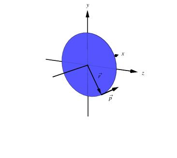
Figure 1: The longitudinal $L_{z}$ (left) and transverse $L_{x}$ (right) components of the orbital angular momentum.

A consequence of this, as will be seen later, is that any sum rule relating the transverse angular momentum of a nucleon to the transverse angular momentum of its constituents, or any division of the total transverse angular momentum into spin and orbital parts, must necessarily involve energy dependent factors, i.e. cannot be frame-independent.

II.4 Lorentz transformation properties of the gauge field $A^{\mu}(x)$ and its consequences

In Classical Electrodynamics, the fields $\bm{E}$ and $\bm{B}$ are physical, and the photon vector potential $A^{\mu}$ largely plays the role of a mathematical aid, i.e. it is often simpler to calculate $A^{\mu}$ than $\bm{E}$ and $\bm{B}$ from the currents and sources, and the physical fields can then be extracted via

$$\bm{E}=-\bm{\nabla}A^{0}-\frac{\partial\bm{A}}{\partial t},\qquad\qquad\bm{B}=\bm{\nabla}\times\bm{A}.$$ (46)

But $A^{\mu}$ is not determined a priori by the currents and sources, since making a classical, local gauge transformation on it

$$A^{\mu}(x)\mapsto\tilde{A}^{\mu}(x)=A^{\mu}(x)+\partial^{\mu}\alpha(x),$$ (47)

where $\alpha(x)$ is any reasonably behaved scalar function, does not alter the physical fields. Thus, in order to carry out any kind of calculation, one has to put some extra condition on $A^{\mu}$, and this is described as choosing a gauge. Now, as its appearance suggests, $A^{\mu}$ is usually treated as a four-vector under Lorentz transformations, but choosing the gauge may contradict this. In Classical Field Theory, one can impose the beautiful Lorenz condition

$$\partial_{\mu}A^{\mu}(x)=0,$$ (48)

which is manifestly covariant and thus does not affect the Lorentz four-vector transformation properties of $A^{\mu}$, and which, moreover, yields uncoupled equations for each component of $A^{\mu}$ in terms of the currents and sources. But sometimes it is more convenient to fix the gauge in some other way. For example, one might use the Coulomb gauge, in which one imposes

$$\bm{\nabla}\cdot\bm{A}(x)=0.$$ (49)

Clearly, this is not a manifestly covariant condition and if it is to hold in all frames, then $A^{\mu}$ cannot transform as a Lorentz four-vector. Indeed, one finds that under a boost of reference frame, $A^{\mu}$ undergoes a combined Lorentz four-vector transformation and a gauge transformation, as explained in section $\bm{14.3}$ of Bjorken:1965zz and in section $\bm{5.9}$ of Weinberg:1995mt . Note that this does not affect the undisputed Lorentz transformation properties of $\bm{E}$ and $\bm{B}$, which follow from Eq. (46) if $A^{\mu}$ transforms as a four-vector, since the extra term, being a gauge transformation, does not affect the electric and magnetic fields.

To construct a Quantum Field Theory, one starts with a classical Lagrangian density. For example, in QED one might begin with the classical Lagrangian density ($e$ is the charge of the electron)

$$\mathcal{L}_{\text{clas}}=-\tfrac{1}{4}\,F_{\mu\nu}F^{\mu\nu}+\tfrac{1}{2}\left[\overline{\psi}(i\,/\!\!\!\!D-m)\psi+\text{h.c.}\right],$$ (50)

where the covariant derivative is defined as

$$D_{\mu}=\partial_{\mu}+ieA_{\mu}.$$ (51)

The Lagrangian in Eq. (50) is invariant under the combined classical, local gauge transformation

$$\psi(x) \mapsto\tilde{\psi}(x)=e^{-ie\alpha(x)}\,\psi(x),$$ (52)

$$A_{\mu}(x) \mapsto\tilde{A}_{\mu}(x)=A_{\mu}(x)+\partial_{\mu}\alpha(x),$$ (53)

but in order to quantize the theory, one has to first choose a gauge. The canonical quantization process amounts to fixing the form of the equal-time commutators between the fields and their conjugates. It is crucial to check that these commutator conditions are compatible with the conditions that fixed the gauge. Unfortunately, it turns out that the canonical commutation relations are incompatible with the operator $A^{\mu}$ satisfying the Lorenz condition. There are several possibilities. One can decide to work in a non-manifestly covariant gauge like the Coulomb gauge, but then one should check that physical quantities thus calculated have the correct Lorentz transformation properties. Or one can work in a manifestly covariant gauge at the expense of introducing additional so-called gauge-fixing fields in QED Lautrup ; Nakanishi:66 and also ghost fields in QCD Kugo:78 . For example, in the Lautrup-Nakanishi covariantly quantized version of QED Lautrup ; Nakanishi:66 , one adds a gauge-fixing part to the classical Lagrangian density in Eq. (50)

$$\mathcal{L}_{\text{gf}}=B(\partial_{\mu}A^{\mu})+\tfrac{\textsf{a}}{2}\,B^{2},$$ (54)

where $B(x)$ is the gauge-fixing field and the parameter a determines the structure of the photon propagator and is irrelevant for the present discussion. $B(x)$ is taken to be unaffected by gauge transformations.

The reason we are emphasizing this is that we will need to write down the most general structure, allowed by symmetry principles, for matrix elements of certain operators like $T^{\mu\nu}$, and this structure will be governed by the transformation properties of the operators. For example, does $T^{\mu\nu}$ transform as a rank-2 Lorentz tensor? Since it is a function of the gauge potential $A^{\mu}$, this will apparently depend on the transformation properties of $A^{\mu}$ imposed by the gauge choice. If $A^{\mu}$ transforms as a Lorentz four-vector, then manifestly $T^{\mu\nu}$ will transform as a second rank tensor, but perhaps surprisingly, as will be discussed in section IV.4, in some cases $T^{\mu\nu}$ will transform as a second rank tensor even though $A^{\mu}$ does not transform as a Lorentz four-vector. It turns out that in most papers this issue has not been recognized, though it is clearly explained in Lorce:2012rr .

II.5 Quantization of a gauge theory

One of the major issues in the controversy about defining quark and gluon angular momentum is the question as to whether a quantity which can be measured experimentally must necessarily be represented in the theory by a gauge-invariant operator. Leader Leader:2011za argued that what one actually measures is the expectation value of an operator, and it can certainly happen that the expectation value of a gauge non-invariant operator, taken between physical states yields a gauge-independent result. The problem is that it seems to be extremely difficult to actually prove such a result for some particular operator. In this section we wish to explain briefly why this is so.

In ordinary Quantum Mechanics in one dimension, the fundamental quantum condition is the canonical commutation relation between the position operator $x$ and its canonical conjugate momentum $p$, namely

$$[x,p]=i\hbar,$$ (55)

where, if $L$ is the Lagrangian,

$$p=\frac{\mathrm{d}L}{\mathrm{d}{\dot{x}}}.$$ (56)

In a Quantum Field Theory, one starts with a Classical Field Theory in which the role of the position operator is played by the fundamental fields $\phi(x)$ and the role of the canonical momentum is played by the conjugate fields $\pi(x)$, defined by

$$\pi=\frac{\partial\mathcal{L}}{\partial(\partial_{0}\phi)},$$ (57)

where $\mathcal{L}$ is the Lagrangian density (we shall henceforth simply refer to it as the “Lagrangian”). To quantize the theory, one tries to mimic Eq. (55) as closely as possible, by imposing the form of the equal-time commutator

$$[\phi(t,\bm{x}),\pi(t,\bm{y})]=i\hbar\,\delta^{(3)}(\bm{x}-\bm{y}).$$ (58)

II.5.1 Problems in the quantization procedure in Gauge Theories

Once $\mathcal{L}$ is chosen, it can happen that $\mathcal{L}$ does not depend on $\partial_{0}\phi$ for some particular field $\phi$, so that its conjugate field is zero, contradicting Eq. (58) for that field. An example is the classical QED Lagrangian given in Eq. (50) which does not contain the variable $\partial_{0}A^{0}$, i.e. there is no momentum conjugate to $A^{0}$.

Just as in Classical Electrodynamics, to actually work with the vector potential $A^{\mu}$, one has to choose a gauge, i.e. impose some condition on $A^{\mu}$, and it may turn out that that condition contradicts the equal-time commutation relations. As an example, consider once again the classical QED Lagrangian given in Eq. (50). Suppose we start with this fully gauge-invariant Lagrangian. Fixing the gauge is tantamount to working with a modified Lagrangian, say $\mathcal{L}^{\prime}$. Such a Lagrangian is known as a gauge-fixed Lagrangian. In principle, there are an infinite number of ways to fix the gauge, so that there are an infinite number of possible gauge-fixed Lagrangians $\mathcal{L}^{\prime},\mathcal{L}^{\prime\prime},\mathcal{L}^{\prime\prime\prime},\cdots$ and the key issue is to show that physical results are the same when working with the various gauge-fixed Lagrangians. For example, to show that $\mathcal{L}^{\prime}$ and $\mathcal{L}^{\prime\prime}$ yield the same result for some physical experimentally measurable quantity $\langle\langle O\rangle\rangle_{\text{phys}}$, one has to show that the expression for $\langle\langle O\rangle\rangle$ does not change under the gauge transformation that changes $\mathcal{L}^{\prime}$ into $\mathcal{L}^{\prime\prime}$, i.e. that $\langle\langle O^{\prime}\rangle\rangle_{\text{phys}}=\langle\langle O^{\prime\prime}\rangle\rangle_{\text{phys}}$.

Now it may happen that the gauge-fixed Lagrangian $\mathcal{L}^{\prime}$ is still invariant under a residual class of gauge transformations. An example is the Lagrangian in the covariantly quantized version of QED due to Lautrup and Nakanishi mentioned earlier, which is a combination of the classical Lagrangian $\mathcal{L}_{\text{clas}}$ in Eq. (50) and the gauge-fixing part $\mathcal{L}_{\text{gf}}$ given in Eq. (54)

$$\mathcal{L}^{\prime}=\mathcal{L}_{\text{clas}}+\mathcal{L}_{\text{gf}}.$$ (59)

The theory is invariant under the residual infinitesimal $c$-number gauge transformation

$$A_{\mu}\mapsto A_{\mu}+\partial_{\mu}\alpha_{\text{res}},\qquad\psi\mapsto\psi-ie\alpha_{\text{res}}\psi,\qquad B\mapsto B,$$ (60)

where, here, $\alpha_{\text{res}}(x)$ is not an arbitrary smooth function, but a function satisfying $\Box\alpha_{\text{res}}\equiv\partial_{\mu}\partial^{\mu}\alpha_{\text{res}}=0$ and vanishing at infinity.

It is of course necessary that $\langle\langle O\rangle\rangle_{\text{phys}}$ does not change under these residual gauge transformations, but that is in no way equivalent to demanding that $\langle\langle O\rangle\rangle_{\text{phys}}$ does not change under the gauge transformation that changes $\mathcal{L}^{\prime}$ into some other $\mathcal{L}^{\prime\prime}$. For example, it was shown in Ref. Leader:2011za that, surprisingly, the total canonical momentum in covariantly quantized QED is not gauge invariant under this residual class of gauge transformations, and it was then proven that its expectation value for physical states is unchanged by such gauge transformations. If the expectation value of the total momentum is a physical quantity, then the latter is certainly necessary, but that is not equivalent to the more demanding requirement of proving that its expectation value is gauge independent.

II.5.2 Gauge invariance vs. gauge independence

One of the least clearly explained concepts in Quantum Field Theory is that of a gauge transformation on a quantum operator. The point is that there is no fully developed theory of operator gauge changes. All the discussion of gauge invariance is based on making classical gauge changes to the fields, i.e. the functions $\alpha_{\text{res}}(x)$ mentioned above, or the more general functions $\alpha(x)$ mentioned in section I, are all ordinary numerical functions, called, in Field Theory, $c$-number functions. Whenever it is stated that a certain operator is gauge invariant, what is meant is that it is invariant under a $c$-number gauge transformation.

Now in a quantum theory, classical dynamical variables are represented by operators, and when we say that we measure a particular dynamical variable, we mean that we measure the expectation value or a physical matrix element of that operator. If then, in our theory, we calculate the value of such a matrix element, its value must not depend upon the choice of gauge we have made in order to carry out the calculation. In other words the matrix elements involved should be gauge independent. Collins (see section $\bm{2.12}$ of Collins:1984xc ) has stressed that it is important to distinguish the concepts of gauge invariance and gauge independence. Gauge invariance is the property of a quantity which does not change under a $c$-number gauge transformation. Gauge independence is a property of a quantum variable whose value does not depend on the method used for fixing the gauge.

It should be clear that demanding gauge independence is not the same as demanding the gauge invariance of the operator, because, as we have emphasized above, gauge invariance of an operator only refers to $c$-number transformations. If, for example, one wanted to compare a calculation in the Coulomb gauge $\bm{\nabla}\cdot\bm{A}=0$ with one in the light-front gauge $A^{+}=0$, one could not make the comparison using gauge invariance, because the corresponding operators $\hat{O}_{\text{Coulomb}}$ and $\hat{O}_{\text{light-front}}$ do not simply differ by a $c$-number function. The easiest way to see this is to note that if you add a $c$-number to an operator, you do not change its commutation relations with other operators, whereas the canonical commutation relations are different in different gauge choices.

So we would need to be able to handle operator-valued gauge transformations, about which almost nothing is known. Several papers in the 1990s (see for example Chen:1998iu ) claimed to prove that the physical matrix elements of the canonical angular momentum operators were gauge independent, using methods very similar to those in Leader:2011za . But unlike the approach in Leader:2011za , it appears that these proofs are valid for a wide class of operator gauge transformations, namely those which are not functions of $\partial_{0}A^{\mu}$ and which therefore commute with $A^{\mu}$. Unfortunately, these papers were considered controversial and never appeared in a journal.

Supposedly, the only safe solution is to express the relevant expectation values in terms of Feynman path integrals, since these involve strictly classical fields. It can be shown e.g. that the physical matrix elements of gauge-invariant operators are gauge independent. However, even this approach is far from clear and has been the subject of much debate, and claims that it can lead to unreliable results Hoodbhoy:1998bt ; Chen:1999kz ; Sun:2000gc . Regrettably we are unable to offer any clarification.

It can happen that the physical matrix elements of a gauge non-invariant operator are gauge independent. Crucially, this means that one cannot automatically demand that every measurable dynamical variable should be represented by a gauge-invariant operator. Indeed, Leader showed in Ref. Leader:2011za that even the total momentum operator in covariantly quantized QED is not invariant under a certain class of $c$-number gauge transformations, yet it ought surely to be a measurable quantity.

II.6 The Belinfante-improved energy-momentum and angular momentum densities

II.6.1 The Belinfante energy-momentum density

As already mentioned, the canonical energy-momentum density $T^{\mu\nu}(x)$ is generally not symmetric under interchange of $\mu$ and $\nu$. It is also not gauge invariant. It is possible to construct from $T^{\mu\nu}(x)$ a so-called Belinfante-improved density $T^{\mu\nu}_{\text{Bel}}(x)$, which is symmetric and which is usually gauge invariant Belinfante:1939 ; Rosenfeld:1940 . It differs from $T^{\mu\nu}(x)$ by a divergence term of the following form:

$$T^{\mu\nu}_{\text{Bel}}\equiv T^{\mu\nu}+\partial_{\lambda}G^{\lambda\mu\nu},$$ (61)

where the so-called superpotential reads

$$G^{\lambda\mu\nu}=\tfrac{1}{2}\left(M^{\lambda\mu\nu}_{\text{spin}}+M^{\mu\nu\lambda}_{\text{spin}}+M^{\nu\mu\lambda}_{\text{spin}}\right),$$ (62)

and, crucially, is antisymmetric w.r.t. its first two indices $G^{\lambda\mu\nu}=-G^{\mu\lambda\nu}$. Alternatively, one can write

$$T^{\mu\nu}_{\text{Bel}}\equiv\tfrac{1}{2}\left(T^{\mu\nu}+T^{\nu\mu}\right)+\tfrac{1}{2}\,\partial_{\lambda}\left(M^{\mu\nu\lambda}_{\text{spin}}+M^{\nu\mu\lambda}_{\text{spin}}\right)$$ (63)

which shows how the Belinfante-improved density generally differs from the symmetric part of the canonical density. The Belinfante-improved density is conserved $\partial_{\mu}T^{\mu\nu}_{\text{Bel}}=0$ and symmetric $T^{\mu\nu}_{\text{Bel}}=T^{\nu\mu}_{\text{Bel}}$. Detailed expressions for $T^{\nu\mu}_{\text{Bel}}$ for QED and QCD will be given in section III.1.

II.6.2 The Belinfante angular momentum density

In a similar way, one can define a Belinfante-improved generalized angular momentum density

$$M^{\mu\nu\rho}_{\text{Bel}}=M^{\mu\nu\rho}+\partial_{\lambda}(x^{\nu}G^{\lambda\mu\rho}-x^{\rho}G^{\lambda\mu\nu}).$$ (64)

Now from Eq. (62), one sees that

$$M^{\mu\nu\rho}_{\text{spin}}=G^{\rho\mu\nu}-G^{\nu\mu\rho}$$ (65)

so that, for the added term in Eq. (64),

$$\partial_{\lambda}(x^{\nu}G^{\lambda\mu\rho}-x^{\rho}G^{\lambda\mu\nu}) =(x^{\nu}\partial_{\lambda}G^{\lambda\mu\rho}-x^{\rho}\partial_{\lambda}G^{\lambda\mu\nu})-(G^{\rho\mu\nu}-G^{\nu\mu\rho})$$

$$=(x^{\nu}\partial_{\lambda}G^{\lambda\mu\rho}-x^{\rho}\partial_{\lambda}G^{\lambda\mu\nu})-M^{\mu\nu\rho}_{\text{spin}}.$$ (66)

It follows from Eq. (64) that

$$M^{\mu\nu\rho}_{\text{Bel}} =M_{\text{OAM}}^{\mu\nu\rho}+(x^{\nu}\partial_{\lambda}G^{\lambda\mu\rho}-x^{\rho}\partial_{\lambda}G^{\lambda\mu\nu})$$

$$=(x^{\nu}T^{\mu\rho}-x^{\rho}T^{\mu\nu})+(x^{\nu}\partial_{\lambda}G^{\lambda\mu\rho}-x^{\rho}\partial_{\lambda}G^{\lambda\mu\nu})$$

$$=x^{\nu}(T^{\mu\rho}+\partial_{\lambda}G^{\lambda\mu\rho}])-x^{\rho}(T^{\mu\nu}+\partial_{\lambda}G^{\lambda\mu\nu})$$

$$=x^{\nu}T^{\mu\rho}_{\text{Bel}}-x^{\rho}T^{\mu\nu}_{\text{Bel}}.$$ (67)

Hence the surprising result that the Belinfante-improved generalized angular momentum density has the structure of a purely orbital angular momentum. It is conserved, $\partial_{\mu}M^{\mu\nu\rho}_{\text{Bel}}=0$, as a consequence of the symmetry of $T^{\mu\nu}_{\text{Bel}}$.

II.6.3 The Belinfante momentum and angular momentum

It follows from Eq. (61) that

$$P^{\mu}_{\text{Bel}} \equiv\int\mathrm{d}^{3}x\,T^{0\mu}_{\text{Bel}}$$

$$=\int\mathrm{d}^{3}x\,T^{0\mu}+\int\mathrm{d}^{3}x\,\partial_{\lambda}G^{\lambda 0\mu}$$

$$=\int\mathrm{d}^{3}x\,T^{0\mu}+\int\mathrm{d}^{3}x\,\partial_{i}G^{i0\mu},$$ (68)

where, in the last line, we used the fact that $G^{00\mu}=0$. Thus, provided that one is allowed to drop the surface term $\int_{V}\mathrm{d}^{3}x\,\partial_{i}G^{i0\mu}=\int_{S}\mathrm{d}^{2}\sigma_{i}\,G^{i0\mu}$, which is tantamount to assuming that the fields vanish at spatial infinity, one has, apparently,

$$P^{\mu}_{\text{Bel}}=P^{\mu}.$$ (69)

Now for a classical $c$-number field, it is meaningful to argue that the field vanishes at infinity and that Eq. (69) holds as a numerical equality. It is much less obvious what this means for a quantum operator. The correct way to tell whether a divergence term can be neglected is to check what its role is in the relevant physical matrix elements involving the operator. In the case of Eq. (69), one can readily check that the matrix elements between any normalizable physical states $|\Phi\rangle$ and $|\Phi^{\prime}\rangle$ are the same, i.e.

$$\langle\Phi^{\prime}|P^{\mu}_{\text{Bel}}|\Phi\rangle=\langle\Phi^{\prime}|P^{\mu}|\Phi\rangle.$$ (70)

However, the operators cannot be identical, because one, for example, may be gauge invariant and the other not, so that the equality would be contradicted upon performing a gauge transformation. On the other hand, the operators are essentially equivalent, and they generate the same transformations on the fields. We feel therefore that Eq. (69) is somewhat misleading and prefer to indicate the equivalence between $P_{\text{Bel}}$ and $P$ as

$$P^{\mu}_{\text{Bel}}\sim P^{\mu}.$$ (71)

It should be noted that it would be impossible to construct a consistent theory if it were not permissible, in certain cases, to ignore the spatial integral of the divergence of a local operator. For example we could not even establish the obvious requirement that the momentum operator commutes with itself! For one has, (no sum over $j$)

$$i\left[P^{j},P^{j}\right]=\int\mathrm{d}^{3}x\,i\left[P^{j},T^{0j}(x)\right]=\int\mathrm{d}^{3}x\,\partial^{j}T^{0j}(x),$$ (72)

where we have used Eq. (16), and this vanishes only if $T^{0j}(x)$ vanishes sufficiently fast at spatial infinity.

The Belinfante angular momentum density leads to the same generalized angular momentum tensor as the canonical one

$$M^{\mu\nu}_{\text{Bel}} =\int\mathrm{d}^{3}x\,M^{0\mu\nu}_{\text{Bel}}$$

$$=\int\mathrm{d}^{3}x\,M^{0\mu\nu}+\int\mathrm{d}^{3}x\,\partial_{i}(x^{\mu}G^{i0\nu}-x^{\nu}G^{i0\mu})$$

$$=M^{\mu\nu},$$ (73)

provided once more that one is allowed to drop the surface term $\int_{V}\mathrm{d}^{3}x\,\partial_{i}[x^{\mu}G^{i0\nu}-x^{\nu}G^{i0\mu}]=\int_{S}\mathrm{d}^{2}\sigma_{i}\,[x^{\mu}G^{i0\nu}-x^{\nu}G^{i0\mu}]$. However, as for the momentum, we prefer to indicate the equivalence of $M^{\mu\nu}$ and $M^{\mu\nu}_{\text{Bel}}$ by

$$M^{\mu\nu}_{\text{Bel}}\sim M^{\mu\nu}.$$ (74)

Operators like $M^{\mu\nu}$, which involve the product of $x$ with a local operator, do not transform like local operators under space-time translations, see Eq. (13), and have been called compound operators in Ref. Bakker:2004ib . For compound operators like the angular momentum, it is a much more difficult task to show the equivalence of the total angular momentum generators $M^{ij}$ and $M^{ij}_{\text{Bel}}$, and care has to be exercised to always use normalizable states. This has been done by Shore and White Shore:1999be .

Interestingly, it seems that as early as 1921, Bessel-Hagen Bessel:1921 found a way to obtain what is now called the Belinfante decomposition, using Noether’s theorem. The trick is to make a combined infinitesimal Lorentz and gauge transformation in the Lagrangian. Such generalized Lorentz transformations are discussed in section IV.4. Recently this trick was rediscovered by Guo and Schmidt Guo:2013jia , who were able to show that all the new decompositions to be discussed in the next few sections could be obtained using Noether’s theorem.

II.6.4 Example of the difference between canonical and Belinfante angular momentum in Classical Electrodynamics

Here is an amusing example, in Classical Electrodynamics, to show that $M^{ij}$ and $M^{ij}_{\text{Bel}}$ or, equivalently, that $\bm{J}$ and $\bm{J}_{\text{Bel}}$ do not always agree with each other. The general expressions for $\bm{J}$ and $\bm{J}_{\text{Bel}}$ in terms of fields will be given in section IV.1. For a free classical electromagnetic field, one has

$$\bm{J}=\underbrace{\int\mathrm{d}^{3}x\,(\bm{E}\times\bm{A})}_{\text{spin term}}+\underbrace{\int\mathrm{d}^{3}x\,E^{i}(\bm{x}\times\bm{\nabla})A^{i}}_{\text{orbital term }}$$ (75)

and

$$\bm{J}_{\text{Bel}}=\int\mathrm{d}^{3}x\left[\bm{x}\times(\bm{E}\times\bm{B})\right].$$ (76)

Consider a left-circularly polarized (= positive helicity) beam, with angular frequency $\omega$, and amplitude proportional to $E_{0}$, propagating along $OZ$, i.e. along the unit vector $\bm{e}_{z}$. Then

$$A^{\mu}=\left(0,\frac{E_{0}}{\omega}\,\cos(kz-\omega t),\frac{E_{0}}{\omega}\,\sin(kz-\omega t),0\right)$$ (77)

gives the correct electric and magnetic fields. $\bm{E}$, $\bm{B}$ and $\bm{A}$ all rotate in the $XY$ plane. Now consider the component of $\bm{J}$ along $OZ$. Note that

$$\bm{\nabla}A_{x,y}\propto\bm{e}_{z}\qquad\text{so that}\qquad(\bm{x}\times\bm{\nabla})_{z}A_{x,y}=0,$$ (78)

so only the spin term contributes to $J_{z}$. One finds

$$J_{z}\text{ per unit volume}=\frac{E_{0}^{2}}{\omega}.$$ (79)

For one photon per unit volume, one requires $E_{0}^{2}=\hbar\omega$ so that

$$J_{z}\text{ per photon}=\hbar$$ (80)

as expected.

For the Belinfante case $\bm{E}\times\bm{B}\propto\bm{e}_{z}$, so that one obtains the incorrect result

$$J_{\text{Bel},z}\text{ per unit volume}=\frac{1}{V}\int\mathrm{d}^{3}x\left[\bm{x}\times(\bm{E}\times\bm{B})\right]_{z}=0\,\,!$$ (81)

Of course, the failure of the two versions to agree with each other is simply due to the fact that the light beam is here described by a plane wave, so that the fields do not vanish at spatial infinity. Computing explicitly the surface integral over the boundary of a cylinder with symmetry axis $\bm{e}_{z}$, one finds for (infinitely) large length $L$ and radius $R$

$$J_{\text{surf},z}=-\pi R^{2}L\,\frac{E^{2}_{0}}{\omega}=-V\,\frac{E^{2}_{0}}{\omega},$$ (82)

which explains why

$$J_{\text{Bel},z}=J_{z}+J_{\text{surf},z}=0.$$ (83)

This example may seem a bit academic, but it is a warning that some care must be utilized when discarding integrals of spatial divergences.

III Detailed structure of the canonical and Belinfante energy-momentum and angular momentum densities

III.1 Structure and Lorentz transformation properties of the energy-momentum density

In section VI, we will need to relate the matrix elements of the angular momentum to the matrix elements of the energy-momentum density. To do this, we will need to write down the most general structure for the matrix elements of $T^{\mu\nu}$, and this will depend upon its behaviour under Lorentz transformations. Major simplifications occur if, as is usually assumed, $T^{\mu\nu}$ transforms as a second-rank Lorentz tensor, but since it is a function of the vector potential $A^{\mu}$, this will only be manifest if $A^{\mu}$ transforms as a Lorentz four-vector. Thus, for simplicity, we are forced to consider covariantly quantized versions of QED and QCD. The problem then is that, besides the electron and photon fields and the quark and gluon fields, one has to introduce gauge-fixing and ghost fields, and these appear in the expressions for $T^{\mu\nu}$. However, in all the recent papers on the angular momentum controversy, with the exception of Leader:2011za , this issue has been completely ignored and the $T^{\mu\nu}$ have been expressed entirely in terms of the electron, photon, quark and gluon fields. In this section we explain why this is actually correct and give explicit expressions for the various versions of the energy-momentum density in terms of the electron, photon, quark and gluon fields.

III.1.1 Structure of the canonical and Belinfante energy-momentum densities in covariantly quantized QED

For covariantly quantized QED, using the Lagrangian given in Eqs. (50) and (54), one finds Leader:2011za for the conserved canonical energy-momentum density

$$T^{\mu\nu}=T^{\mu\nu}_{\text{clas}}+T^{\mu\nu}_{\text{gf}},$$ (84)

where

$$T^{\mu\nu}_{\text{clas}} =\tfrac{1}{2}\,\overline{\psi}\gamma^{\mu}i\overset{\leftrightarrow}{\partial}\!\!\!\!\phantom{\partial}^{\nu}\psi-F^{\mu\alpha}\partial^{\nu}A_{\alpha}-g^{\mu\nu}{\cal{L}}_{\text{clas}},$$ (85)

$$T^{\mu\nu}_{\text{gf}} =B\,\partial^{\nu}A^{\mu}-g^{\mu\nu}\mathcal{L}_{\text{gf}}$$ (86)

with $\overset{\leftrightarrow}{\partial}\!\!\!\!\phantom{\partial}^{\nu}\equiv\overset{\rightarrow}{\partial}\!\!\!\!\phantom{\partial}^{\nu}-\overset{\leftarrow}{\partial}\!\!\!\!\phantom{\partial}^{\nu}$.

For the conserved Belinfante density, one finds

$$T^{\mu\nu}_{\text{Bel}}=T^{\mu\nu}_{\text{Bel,clas}}+T^{\mu\nu}_{\text{Bel,gf}},$$ (87)

where

$$T^{\mu\nu}_{\text{Bel,clas}} =\tfrac{1}{4}\,\overline{\psi}(\gamma^{\mu}i\overset{\leftrightarrow}{D}\!\!\!\!\!\phantom{D}^{\nu}+\gamma^{\nu}i\overset{\leftrightarrow}{D}\!\!\!\!\!\phantom{D}^{\mu})\psi-F^{\mu\alpha}F^{\nu}_{\phantom{\nu}\alpha}-g^{\mu\nu}\mathcal{L}_{\text{clas}},$$ (88)

$$T^{\mu\nu}_{\text{Bel,gf}} =-(\partial^{\mu}B)A^{\nu}-(\partial^{\nu}B)A^{\mu}-g^{\mu\nu}{\cal{L}}_{\text{gf}},$$ (89)

where $\overset{\leftrightarrow}{D}\!\!\!\!\!\phantom{D}^{\nu}=\overset{\leftrightarrow}{\partial}\!\!\!\!\phantom{\partial}^{\nu}+2ieA^{\nu}$.

The conservation of an energy-momentum density depends on the equations of motion, which are a consequence of the Lagrangian. Thus, for example, $T^{\mu\nu}_{\text{Bel}}$ is conserved, but $T^{\mu\nu}_{\text{Bel,clas}}$ is not, when the Lagrangian is $\mathcal{L}_{\text{clas}}+\mathcal{L}_{\text{gf}}$. On the other hand, $T^{\mu\nu}_{\text{Bel,clas}}$ would be conserved if the Lagrangian were $\mathcal{L}_{\text{clas}}$. Now often in the literature, the Belinfante energy-momentum density is simply taken to be $T^{\mu\nu}_{\text{Bel,clas}}$ and is treated as if it were conserved, i.e. the momentum operator based on it is taken to be independent of time (equivalently: to remain unrenormalized), which would imply that the Lagrangian is just $\mathcal{L}_{\text{clas}}$. But it is well known that one cannot quantize QED covariantly using just $\mathcal{L}_{\text{clas}}$. It turns out, however, that this is innocuous, since it can be shown Leader:2011za that for physical matrix elements, for both the canonical and Belinfante versions,

$$\langle\Phi^{\prime}|T^{\mu\nu}_{\text{gf}}|\Phi\rangle=\langle\Phi^{\prime}|T^{\mu\nu}_{\text{Bel,gf}}|\Phi\rangle=0.$$ (90)

Hence

$$\begin{split}\langle\Phi^{\prime}|\,\partial_{\mu}T^{\mu\nu}_{\text{clas}}|\Phi\rangle&=\langle\Phi^{\prime}|\,\partial_{\mu}T^{\mu\nu}|\Phi\rangle=0,\\ \langle\Phi^{\prime}|\partial_{\mu}T^{\mu\nu}_{\text{Bel,clas}}|\Phi\rangle&=\langle\Phi^{\prime}|\,\partial_{\mu}T^{\mu\nu}_{\text{Bel}}|\Phi\rangle=0.\end{split}$$ (91)

In summary, covariant quantization of QED complicates some aspects and there is no compelling reason to insist on it. Indeed, the non-manifestly covariant Coulomb gauge leads to a perfectly good Lorentz-invariant theory. However, for our purposes it is helpful to work with a covariantly quantized theory, and since we will only consider physical matrix elements, $T^{\mu\nu}_{\text{clas}}$ and $T^{\mu\nu}_{\text{Bel,clas}}$ may be treated as conserved tensor operators. Consequently, in the following, we may take

$$T^{\mu\nu} \sim T^{\mu\nu}_{\text{clas}},$$ (92)

$$T^{\mu\nu}_{\text{Bel}} \sim T^{\mu\nu}_{\text{Bel,clas}}.$$ (93)

III.1.2 Structure of the canonical and Belinfante energy-momentum densities in covariantly quantized QCD

The situation in QCD is somewhat more complicated. The infinitesimal gauge transformations on the gluon vector potential and on the quark fields, under which the pure quark-gluon Lagrangian $\mathcal{L}_{\textrm{QCD}}$ (the QCD analogue of the QED $\mathcal{L}_{\text{clas}})$

$$\mathcal{L}_{\textrm{QCD}}=\mathcal{L}_{\textrm{D}}+\mathcal{L}_{\textrm{YM}}+\mathcal{L}_{\textrm{int}},$$ (94)

where the Dirac (D), Yang-Mills (YM) and interaction terms (int) are given by

$$\mathcal{L}_{\text{D}} =\overline{\psi}_{r}(\tfrac{i}{2}\,/\!\!\!\!\overset{\leftrightarrow}{\partial}\!\!\!\!\phantom{\partial}-m)\delta_{rs}\psi_{s},$$ (95)

$$\mathcal{L}_{\text{YM}} =-\tfrac{1}{4}\,G^{a}_{\mu\nu}G^{\mu\nu}_{a},$$ (96)

$$\mathcal{L}_{\text{int}} =g\,\overline{\psi}_{r}\,/\!\!\!\!A^{a}t^{a}_{rs}\psi_{s},$$ (97)

is invariant, are determined by eight scalar $c$-number fields $\theta^{a}(x)$,

$$\delta A^{a}_{\mu}(x) =\left[\partial_{\mu}\,\delta^{ab}-gf^{abc}A^{c}_{\mu}(x)\right]\theta^{b}(x)\equiv D^{ab}_{\mu}\theta^{b}(x),$$ (98)

$$\delta\psi_{r}(x) =ig\theta^{a}(x)t^{a}_{rs}\psi_{s}(x).$$ (99)

Here $a,b,c=1,2...8$ and $r,s=1,2,3$ are color labels, the matrices $t^{a}$ satisfy $[t^{a},t^{b}]=if^{abc}t^{c}$, and the gluon field-strength tensor is given by

$$G^{a}_{\mu\nu}=\partial_{\mu}A^{a}_{\nu}-\partial_{\nu}A^{a}_{\mu}+gf^{abc}A^{b}_{\mu}A^{c}_{\nu}.$$ (100)

A sum over quark flavors is to be understood here and in what follows.

However, in order to quantize the theory covariantly, one has to introduce both a gauge-fixing field $B(x)$ and Faddeev-Popov anti-commuting fermionic ghost fields $c(x)$ and $\overline{c}(x)$. The Kugo-Ojima Lagrangian Kugo:78 for the covariantly quantized theory is then

$$\mathcal{L}=\mathcal{L}_{\textrm{QCD}}+\mathcal{L}_{\text{gf}+\text{gh}},$$ (101)

where

$$\mathcal{L}_{\text{gf}+\text{gh}}=-i(\partial^{\mu}\overline{c}^{a})D^{ab}_{\mu}c^{b}-(\partial^{\mu}B^{a})A^{a}_{\mu}+\tfrac{\textsf{a}}{2}\,B^{a}B^{a}$$ (102)

with a a parameter which fixes the structure of the gluon propagator, and which is irrelevant for the present discussion. The extra term $\mathcal{L}_{\text{gf}+\text{gh}}$ is not invariant under the original infinitesimal gauge transformations given by Eqs. (98) and (99). Instead the theory is invariant under the BRST transformations Becchi:1975nq ; *Tyutin

$$\begin{split}\delta A^{a}_{\mu}(x)&=\theta D^{ab}_{\mu}c^{b}(x),\\ \delta\psi_{r}(x)&=ig\theta\,t^{a}_{rs}c^{a}(x)\psi_{s}(x),\\ \delta c^{a}(x)&=-\tfrac{g}{2}\,\theta f^{abc}c^{b}(x)c^{c}(x),\\ \delta\overline{c}^{a}(x)&=i\theta B^{a}(x),\\ \delta B(x)&=0,\end{split}$$ (103)

where $\theta$ is a constant operator which commutes with bosonic fields and anti-commutes with fermionic fields. The BRST transformation is generated by $\theta Q_{B}$, i.e. for any of the above fields $\phi$

$$i[\theta Q_{B},\phi]=\delta\phi,$$ (104)

where the conserved, hermitian charge $Q_{B}$ is given by

$$Q_{B}=\int\mathrm{d}^{3}x\left[B^{a}\overset{\leftrightarrow}{\partial}\!\!\!\!\phantom{\partial}_{0}c^{a}+gB^{a}f^{abc}A^{b}_{0}c^{c}+i\tfrac{g}{2}\,(\partial_{0}\overline{c}^{a})f^{abc}c^{b}c^{c}\right].$$ (105)

There is also a conserved charge

$$Q_{c}=\int\mathrm{d}^{3}x\left[\overline{c}^{a}\overset{\leftrightarrow}{\partial}\!\!\!\!\phantom{\partial}_{0}c^{a}+g\overline{c}^{a}f^{abc}A^{b}_{0}c^{c}\right]$$ (106)

which “measures” the ghost number

$$i[Q_{c},\phi]=N\phi,$$ (107)

where $N=1$ for $\phi=c$, $-1$ for $\phi=\overline{c}$ and $0$ for all other fields. The physical states $|\Phi\rangle$ are defined by the subsidiary conditions

$$Q_{B}|\Phi\rangle=0,\qquad\qquad Q_{c}|\Phi\rangle=0.$$ (108)

One finds for the canonical energy-momentum tensor density

$$T^{\mu\nu}=T^{\mu\nu}_{\textrm{QCD}}+T^{\mu\nu}_{\text{gf}+\text{gh}},$$ (109)

where

$$T^{\mu\nu}_{\textrm{QCD}} =\tfrac{1}{2}\,\overline{\psi}_{r}\gamma^{\mu}i\overset{\leftrightarrow}{\partial}\!\!\!\!\phantom{\partial}^{\nu}\psi_{r}-G^{\mu\alpha}_{a}\partial^{\nu}A^{a}_{\alpha}-g^{\mu\nu}\mathcal{L}_{\textrm{QCD}},$$ (110)

$$T^{\mu\nu}_{\textrm{gf+gh}} =-A^{\mu}_{a}\partial^{\nu}B^{a}-i(\partial^{\nu}\overline{c}^{a})D^{\mu}_{ab}c^{b}-i(\partial^{\mu}\overline{c}^{a})(\partial^{\nu}c^{a})-g^{\mu\nu}\mathcal{L}_{\text{gf}+\text{gh}}.$$ (111)

The Belinfante version is

$$T^{\mu\nu}_{\text{Bel}}=T^{\mu\nu}_{\text{Bel},\textrm{QCD}}+T^{\mu\nu}_{\text{Bel,gf}+\text{gh}},$$ (112)

where

$$T^{\mu\nu}_{\text{Bel},\textrm{QCD}}=\tfrac{1}{4}\,\overline{\psi}_{r}(\gamma^{\mu}i\overset{\leftrightarrow}{D}\!\!\!\!\!\phantom{D}^{\nu}_{rs}+\gamma^{\nu}i\overset{\leftrightarrow}{D}\!\!\!\!\!\phantom{D}^{\mu}_{rs})\psi_{s}-G^{\mu\alpha}_{a}G^{a\nu}_{\phantom{a\nu}\alpha}-g^{\mu\nu}\mathcal{L}_{\textrm{QCD}}$$ (113)

is BRST invariant, i.e. commutes with $Q_{B}$. Here $\overset{\leftrightarrow}{D}\!\!\!\!\!\phantom{D}^{\nu}_{rs}$ is a matrix in color space

$$\overset{\leftrightarrow}{D}\!\!\!\!\!\phantom{D}^{\nu}_{rs}=\overset{\leftrightarrow}{\partial}\!\!\!\!\phantom{\partial}^{\nu}\delta_{rs}-2igA^{\nu}_{a}t^{a}_{rs}.$$ (114)

The gauge-fixing and ghost terms are given by

$$T^{\mu\nu}_{\text{Bel,gf}+\text{gh}}=-(A^{\mu}_{a}\partial^{\nu}B^{a}+A^{\nu}_{a}\partial^{\mu}B^{a})-i[(\partial^{\mu}\overline{c}^{a})D^{\nu}_{ab}c^{b}+(\partial^{\nu}\overline{c}^{a})D^{\mu}_{ab}c^{b}]-g^{\mu\nu}\mathcal{L}_{\text{gf}+\text{gh}}.$$ (115)

This can be rewritten as an anti-commutator with $Q_{B}$ Kugo:1979gm

$$T^{\mu\nu}_{\text{Bel,gf}+\text{gh}}=-\left\{Q_{B},\left[(\partial^{\mu}\overline{c}^{a})A^{\nu}_{a}+(\partial^{\nu}\overline{c}^{a})A^{\mu}_{a}+g^{\mu\nu}\left(\tfrac{\textsf{a}}{2}\,\overline{c}^{a}B^{a}-(\partial^{\rho}\overline{c}^{a})A^{a}_{\rho}\right)\right]\right\}.$$ (116)

It follows that $T^{\mu\nu}_{\text{Bel,gf}+\text{gh}}$ is BRST invariant (because $Q_{B}$ is nilpotent, i.e. $Q_{B}^{2}=0$) and does not contribute to physical matrix elements

$$\langle\Phi^{\prime}|T^{\mu\nu}_{\text{Bel}}|\Phi\rangle=\langle\Phi^{\prime}|T^{\mu\nu}_{\text{Bel},\textrm{QCD}}|\Phi\rangle.$$ (117)

The situation with the canonical energy-momentum tensor $T^{\mu\nu}$ is somewhat more complicated, but it can be shown Leader:2011za that contrary to the statement in Ref. Shore:1999be , $T^{\mu\nu}_{\text{gf}+\text{gh}}$ does not contribute to physical matrix elements.

Consequently, analogous to the QED case, in the following we may use

$$T^{\mu\nu} \sim T^{\mu\nu}_{\textrm{QCD}},$$ (118)

$$T^{\mu\nu}_{\text{Bel}} \sim T^{\mu\nu}_{\text{Bel},\textrm{QCD}},$$ (119)

where, we remind the reader, a sum over quark flavors is implied.

We can now define separate quark and gluon parts of $T^{\mu\nu}$:

$$T^{\mu\nu}_{q} \sim\tfrac{1}{2}\,\overline{\psi}_{r}\gamma^{\mu}i\overset{\leftrightarrow}{\partial}\!\!\!\!\phantom{\partial}^{\nu}\psi_{r}-g^{\mu\nu}\mathcal{L}_{\text{D }},$$ (120)

$$T^{\mu\nu}_{G} \sim-G^{\mu\alpha}_{a}\partial^{\nu}A^{a}_{\alpha}-g^{\mu\nu}(\mathcal{L}_{\text{YM}}+\mathcal{L}_{\text{int}}),$$ (121)

and similarly, for $T^{\mu\nu}_{\text{Bel}}$:

$$T^{\mu\nu}_{\text{Bel},q} \sim\tfrac{1}{4}\,\overline{\psi}_{r}(\gamma^{\mu}i\overset{\leftrightarrow}{D}\!\!\!\!\!\phantom{D}^{\nu}_{rs}+\gamma^{\nu}i\overset{\leftrightarrow}{D}\!\!\!\!\!\phantom{D}^{\mu}_{rs})\psi_{s}-g^{\mu\nu}(\mathcal{L}_{\text{D}}+\mathcal{L}_{\text{int}}),$$ (122)

$$T^{\mu\nu}_{\text{Bel},G} \sim-G^{\mu\alpha}_{a}G^{a\nu}_{\phantom{a\nu}\alpha}-g^{\mu\nu}\mathcal{L}_{\text{YM}}.$$ (123)

Note that for considerations of the genuine angular momentum, one always has $\mu\neq\nu$, so the terms proportional to $g^{\mu\nu}$ are irrelevant.

III.2 Structure of the angular momentum operators in QED

In this section we give a pedagogical demonstration of how the principal angular momentum operators are derived from the corresponding expressions for the energy-momentum tensors, given above. So as not to drown the essential ideas in a mass of algebra, we shall limit ourselves to QED. The derivation for QCD is similar but more tedious.

III.2.1 The Belinfante angular momentum in QED and the form used by Ji

According to Eq. (II.6.2), the Belinfante angular momentum is given by

$$M^{jk}_{\text{Bel}}=\int\mathrm{d}^{3}x\,M^{0jk}_{\text{Bel}}(x),$$ (124)

where

$$M^{\mu\nu\rho}_{\text{Bel}}=x^{\nu}T^{\mu\rho}_{\text{Bel}}-x^{\rho}T^{\mu\nu}_{\text{Bel}}.$$ (125)

For QED, the electron part of this is, from Eq. (88) and keeping only the relevant terms for the actual angular momentum,

$$M^{\mu\nu\rho}_{\text{Bel},e}=x^{\nu}\,\tfrac{1}{4}\,\overline{\psi}(\gamma^{\mu}i\overset{\leftrightarrow}{D}\!\!\!\!\!\phantom{D}^{\rho}+\gamma^{\rho}i\overset{\leftrightarrow}{D}\!\!\!\!\!\phantom{D}^{\mu})\psi-(\nu\leftrightarrow\rho),$$ (126)

and is not split into a spin part and orbital part. Such a split can be achieved as follows. We can write

$$\tfrac{1}{4}\,\overline{\psi}(\gamma^{\mu}i\overset{\leftrightarrow}{D}\!\!\!\!\!\phantom{D}^{\nu}+\gamma^{\nu}i\overset{\leftrightarrow}{D}\!\!\!\!\!\phantom{D}^{\mu})\psi=\tfrac{1}{2}\,\overline{\psi}\gamma^{\mu}i\overset{\leftrightarrow}{D}\!\!\!\!\!\phantom{D}^{\nu}\psi+\tfrac{1}{4}\,\overline{\psi}(\gamma^{\nu}i\overset{\leftrightarrow}{D}\!\!\!\!\!\phantom{D}^{\mu}-\gamma^{\mu}i\overset{\leftrightarrow}{D}\!\!\!\!\!\phantom{D}^{\nu})\psi.$$ (127)

Then, using the following gamma matrix identities ($\epsilon_{0123}=1$)

$$\begin{split}\sigma^{\mu\nu}\gamma^{\rho}&=ig^{\nu\rho}\gamma^{\mu}-ig^{\mu\rho}\gamma^{\nu}+\epsilon^{\mu\nu\rho\sigma}\gamma_{\sigma}\gamma_{5},\\ \gamma^{\rho}\sigma^{\mu\nu}&=ig^{\mu\rho}\gamma^{\nu}-ig^{\nu\rho}\gamma^{\mu}+\epsilon^{\mu\nu\rho\sigma}\gamma_{\sigma}\gamma_{5},\end{split}$$ (128)

and multiplying the first by $i\overset{\rightarrow}{D}\!\!\!\!\!\phantom{D}_{\rho}=i\overset{\rightarrow}{\partial}\!\!\!\!\phantom{\partial}_{\rho}-eA_{\rho}$ and the second by $i\overset{\leftarrow}{D}\!\!\!\!\!\phantom{D}_{\rho}=i\overset{\leftarrow}{\partial}\!\!\!\!\phantom{\partial}_{\rho}+eA_{\rho}$, one obtains

$$\begin{split}\sigma^{\mu\nu}i\,/\!\!\!\!\overset{\rightarrow}{D}\!\!\!\!\!\phantom{D}&=\gamma^{\nu}\overset{\rightarrow}{D}\!\!\!\!\!\phantom{D}^{\mu}-\gamma^{\mu}\overset{\rightarrow}{D}\!\!\!\!\!\phantom{D}^{\nu}+i\,\epsilon^{\mu\nu\rho\sigma}\gamma_{\sigma}\gamma_{5}\overset{\rightarrow}{D}\!\!\!\!\!\phantom{D}_{\rho},\\ i\,/\!\!\!\!\overset{\leftarrow}{D}\!\!\!\!\!\phantom{D}\,\sigma^{\mu\nu}&=\overset{\leftarrow}{D}\!\!\!\!\!\phantom{D}^{\nu}\gamma^{\mu}-\overset{\leftarrow}{D}\!\!\!\!\!\phantom{D}^{\mu}\gamma^{\nu}+i\,\epsilon^{\mu\nu\rho\sigma}\gamma_{\sigma}\gamma_{5}\overset{\leftarrow}{D}\!\!\!\!\!\phantom{D}_{\rho}.\end{split}$$ (129)

Sandwiching these between $\overline{\psi}$ and $\psi$ and using the equations of motion for the electron field $i\,/\!\!\!\!\overset{\rightarrow}{D}\!\!\!\!\!\phantom{D}\psi=m\psi$ and $i\overline{\psi}\,/\!\!\!\!\overset{\leftarrow}{D}\!\!\!\!\!\phantom{D}=-m\overline{\psi}$, one obtains the useful identity

$$\overline{\psi}(\gamma^{\nu}i\overset{\leftrightarrow}{D}\!\!\!\!\!\phantom{D}^{\mu}-\gamma^{\mu}i\overset{\leftrightarrow}{D}\!\!\!\!\!\phantom{D}^{\nu})\psi=\epsilon^{\mu\nu\rho\sigma}\partial_{\rho}\!\left(\overline{\psi}\gamma_{\sigma}\gamma_{5}\psi\right),$$ (130)

which is consistent with the generic form given in Eq. (40). The contribution of the antisymmetric term in Eq. (127) to $M^{jk}_{\text{Bel},e}$ is then

$$\int\mathrm{d}^{3}x\,x^{j}\,\tfrac{1}{4}\,\overline{\psi}(\gamma^{k}i\overset{\leftrightarrow}{D}\!\!\!\!\!\phantom{D}^{0}-\gamma^{0}i\overset{\leftrightarrow}{D}\!\!\!\!\!\phantom{D}^{k})\psi-(j\leftrightarrow k) =\tfrac{1}{4}\,\epsilon^{0k\rho\sigma}\int\mathrm{d}^{3}x\,x^{j}\partial_{\rho}\!\left(\overline{\psi}\gamma_{\sigma}\,\gamma_{5}\psi\right)-(j\leftrightarrow k)$$

$$=\tfrac{1}{4}\,\epsilon^{0k\rho\sigma}\int\mathrm{d}^{3}x\left[\partial_{\rho}\!\left(x^{j}\,\overline{\psi}\gamma_{\sigma}\gamma_{5}\psi\right)-\delta^{j}_{\rho}\,\overline{\psi}\gamma_{\sigma}\gamma_{5}\psi\right]-(j\leftrightarrow k)$$

$$=\tfrac{1}{2}\,\epsilon^{jkl}\int\mathrm{d}^{3}x\,\overline{\psi}\gamma^{l}\gamma_{5}\psi$$

$$=\tfrac{1}{2}\int\mathrm{d}^{3}x\,\psi^{\dagger}\sigma^{jk}\psi,$$ (131)

where we have discarded the integral of a spatial divergence. The contribution to $M^{jk}_{\text{Bel},e}$ from the first term on the RHS of Eq. (127) is

$$\tfrac{1}{2}\int\mathrm{d}^{3}x\,x^{j}\,\overline{\psi}\gamma^{0}i\overset{\leftrightarrow}{D}\!\!\!\!\!\phantom{D}^{k}\psi-(j\leftrightarrow k)=\int\mathrm{d}^{3}x\,\psi^{\dagger}x^{j}iD^{k}\psi-(j\leftrightarrow k),$$ (132)

where, again, we have discarded a surface term. Finally then, from Eqs. (III.2.1) and (132), $J^{i}_{\text{Bel},e}=\tfrac{1}{2}\,\epsilon^{ijk}M^{jk}_{\text{Bel},e}$ can be written in the form of a spin term plus an orbital term in the form used by Ji

$$\bm{J}^{e}_{\text{Ji}}=\int\mathrm{d}^{3}x\,\psi^{\dagger}\tfrac{1}{2}\bm{\Sigma}\psi+\int\mathrm{d}^{3}x\,\psi^{\dagger}(\bm{x}\times i\bm{D})\psi,$$ (133)

where we have used Eq. (27). We shall refer to the above terms as $\bm{S}^{e}_{\text{Ji}}$ and $\bm{L}^{e}_{\text{Ji}}$, respectively. The photon part of the Belinfante angular momentum follows directly upon substituting in terms of the electric and magnetic fields, i.e. using $F^{i0}=E^{i}$ and $F^{ij}=-\epsilon^{ijk}B^{k}$, and one arrives at the Ji decomposition:

$$\bm{J}_{\text{QED}}=\underbrace{\int\mathrm{d}^{3}x\,\psi^{\dagger}\tfrac{1}{2}\bm{\Sigma}\psi}_{\bm{S}^{e}_{\text{Ji}}}+\underbrace{\int\mathrm{d}^{3}x\,\psi^{\dagger}(\bm{x}\times i\bm{D})\psi}_{\bm{L}^{e}_{\text{Ji}}}+\underbrace{\int\mathrm{d}^{3}x\,\bm{x}\times(\bm{E}\times\bm{B})}_{\bm{J}^{\gamma}_{\text{Ji}}},$$ (134)

which will be discussed in section IV.1. Here and everywhere in the following, $e$ means electron plus positron.

III.2.2 The canonical angular momentum in QED used by Jaffe and Manohar

As explained in section II.2.2, the canonical angular momentum density is automatically split into orbital and spin parts for both electrons and photons. From Eqs. (37) and (85), the electron orbital angular momentum density is given by

$$M^{0jk}_{e,\text{OAM}}=\tfrac{1}{2}\,x^{j}(\overline{\psi}\gamma^{0}i\overset{\leftrightarrow}{\partial}\!\!\!\!\phantom{\partial}^{k}\psi)-(j\leftrightarrow k)=\psi^{\dagger}x^{j}i\partial^{k}\psi-(j\leftrightarrow k)\,+\,\text{divergence term}.$$ (135)

The photon orbital angular momentum density is given by

$$M^{0jk}_{\gamma,\text{OAM}} =-x^{j}F^{0l}\partial^{k}A_{l}-(j\leftrightarrow k)$$

$$=x^{j}E^{l}\partial^{k}A_{l}-(j\leftrightarrow k)$$

$$=E^{l}x^{j}\nabla^{k}A^{l}-(j\leftrightarrow k).$$ (136)

The electron spin density term, from Eqs. (38) and (22) reads

$$M^{0jk}_{e,\text{spin}} =-i\,\frac{\partial\mathcal{L}_{\text{clas}}}{\partial(\partial_{0}\psi_{r})}\,\tfrac{1}{2}(\sigma^{jk})^{\phantom{r}s}_{r}\psi_{s}$$

$$=\psi^{\dagger}\tfrac{1}{2}\sigma^{jk}\psi,$$ (137)

where $r$ and $s$ are here Dirac spinor indices, and where we have used $\frac{\partial\mathcal{L}_{\text{clas}}}{\partial(\partial_{0}\psi_{r})}=i\psi^{{\dagger}r}$. Finally, the photon spin density term is, from Eqs. (23) and (38)

$$M^{0jk}_{\gamma,\text{spin}} =-i\,\frac{\partial\mathcal{L}_{\text{clas}}}{\partial(\partial_{0}A_{\alpha})}\,i(\delta^{j}_{\alpha}\,g^{k\beta}-\delta^{k}_{\alpha}\,g^{j\beta})A_{\beta}$$

$$=\frac{\partial\mathcal{L}_{\text{clas}}}{\partial(\partial_{0}A_{j})}\,A^{k}-(j\leftrightarrow k)$$

$$=E^{j}A^{k}-E^{k}A^{j},$$ (138)

where we have used $\frac{\partial\mathcal{L}_{\text{clas}}}{\partial(\partial_{0}A_{j})}=E^{j}$. Putting these together to form $J^{i}_{\text{QED}}=\tfrac{1}{2}\,\epsilon^{ijk}M^{jk}$, one obtains the canonical form of the QED angular momentum used by Jaffe and Manohar:

$$\bm{J}_{\text{QED}}=\underbrace{\int\mathrm{d}^{3}x\,\psi^{\dagger}\tfrac{1}{2}\bm{\Sigma}\psi}_{\bm{S}^{e}_{\text{JM}}}+\underbrace{\int\mathrm{d}^{3}x\,\psi^{\dagger}(\bm{x}\times\tfrac{1}{i}\bm{\nabla})\psi}_{\bm{L}^{e}_{\text{JM}}}+\underbrace{\int\mathrm{d}^{3}x\,\bm{E}\times\bm{A}}_{\bm{S}^{\gamma}_{\text{JM}}}+\underbrace{\int\mathrm{d}^{3}x\,E^{i}(\bm{x}\times\bm{\nabla})A^{i}}_{\bm{L}^{\gamma}_{\text{JM}}},$$ (139)

which will be discussed in section IV.1.

IV The controversy in detail

To keep the presentation as simple as possible, we consider in this section the case of QED. The expressions for more general gauge theories, including QCD, will be given in the next section. We confine also our discussions mainly to Classical Field Theory, so that we can spare the complications originating from the quantization procedure. Whenever we refer to quantum operators, these correspond to the naive operators obtained by replacing the classical fields in the classical expressions by their quantum counterpart. Note that, to the best of our knowledge, a proper and complete treatment at the quantum level has unfortunately never been achieved in the literature.

IV.1 The main decompositions of the angular momentum in a nutshell

Here, we present and compare the main different decompositions of the angular momentum proposed in the literature and comment on their advantages and disadvantages. Similar decompositions exist for the linear momentum and most of our discussions can easily be transposed.

IV.1.1 The Belinfante decomposition

As shown in Eq. (II.6.2), the Belinfante angular momentum density has a purely orbital appearance, and following the procedure utilized by Belinfante and Rosenfeld Belinfante:1939 ; Rosenfeld:1940 , one explicitly obtains the following decomposition

$$\bm{J}_{\text{QED}}=\underbrace{\int\mathrm{d}^{3}x\,\overline{\psi}\left[\bm{x}\times\tfrac{1}{2}\,(\gamma^{0}\,i\bm{D}+\bm{\gamma}\,iD^{0})\right]\psi}_{\bm{J}^{e}_{\text{Bel}}}+\underbrace{\int\mathrm{d}^{3}x\,\bm{x}\times(\bm{E}\times\bm{B})}_{\bm{J}^{\gamma}_{\text{Bel}}},$$ (140)

where the covariant derivative is given by $\bm{D}=\bm{\partial}+ie\bm{A}\equiv-\bm{\nabla}+ie\bm{A}$ and $D^{0}=\partial_{t}+ieA^{0}$ in accordance with Eq. (51). The quantities $\bm{J}^{e}_{\text{Bel}}$ and $\bm{J}^{\gamma}_{\text{Bel}}$ are interpreted as the electron and photon total angular momentum, respectively.

Advantages

• Each separate term is a gauge-invariant quantity and therefore measurable in principle;

Disadvantages

• There is no decomposition of the total angular momentum into spin and OAM contributions;

• The individual contributions $\bm{J}^{e}_{\text{Bel}}$ and $\bm{J}^{\gamma}_{\text{Bel}}$, seen as operators, do not satisfy the generic equal-time commutation relations $[J^{i},J^{j}]=i\epsilon^{ijk}J^{k}$ defining angular momentum operators in a quantum theory;

• $\bm{J}^{e}_{\text{Bel}}$ and $\bm{J}^{\gamma}_{\text{Bel}}$ are not generators of rotations.

IV.1.2 The Ji decomposition

In section III.2.1, we showed how the Belinfante angular momentum could be rewritten in such a way that the electron angular momentum was split into a sum of a spin and orbital term. This is the form used by Ji in his seminal paper relating the quark and gluon angular momenta to GPDs and, following the tradition in the literature, we shall therefore refer to it as the “Ji decomposition”. One has thus

$$\bm{J}_{\text{QED}}=\underbrace{\int\mathrm{d}^{3}x\,\psi^{\dagger}\tfrac{1}{2}\bm{\Sigma}\psi}_{\bm{S}^{e}_{\text{Ji}}}+\underbrace{\int\mathrm{d}^{3}x\,\psi^{\dagger}(\bm{x}\times i\bm{D})\psi}_{\bm{L}^{e}_{\text{Ji}}}+\underbrace{\int\mathrm{d}^{3}x\,\bm{x}\times(\bm{E}\times\bm{B})}_{\bm{J}^{\gamma}_{\text{Ji}}}.$$ (141)

Interestingly, this decomposition can be obtained by adding the surface term $-\int\mathrm{d}^{3}x\,\nabla^{i}[E^{i}(\bm{x}\times\bm{A})]$ to the Jaffe-Manohar decomposition given in the next subsection, and by using the equation of motion $\bm{\nabla}\cdot\bm{E}=e\psi^{\dagger}\psi$. The quantities $\bm{S}^{e}_{\text{Ji}}$, $\bm{L}^{e}_{\text{Ji}}$, and $\bm{J}^{\gamma}_{\text{Ji}}$ are interpreted as the electron spin, electron OAM, and photon total angular momentum, respectively.

Advantages

• Each separate term is a gauge-invariant quantity and therefore measurable in principle;

• The presence of the covariant derivative $\bm{D}=-\bm{\nabla}+ie\bm{A}$ suggests that the electron OAM $\bm{L}^{e}_{\text{Ji}}$ is kinetic, i.e. corresponds to the classical definition $\bm{x}\times\bm{p}_{\text{kin}}$, where $\bm{p}_{\text{kin}}=m\bm{v}$ with $\bm{v}$ the velocity of the particle, according to the common understanding of Classical Electrodynamics;

• The photon total angular momentum coincides with the corresponding Belinfante expression $\bm{J}^{\gamma}_{\text{Ji}}=\bm{J}^{\gamma}_{\text{Bel}}$. This holds also for the electron total angular momentum $\bm{S}^{e}_{\text{Ji}}+\bm{L}^{e}_{\text{Ji}}=\bm{J}^{e}_{\text{Bel}}$ up to a surface term. The Ji decomposition generalizes therefore the Belinfante decomposition by providing an explicit gauge-invariant decomposition of the electron total angular momentum into spin and OAM contributions up to a surface term.

Disadvantages

• There is no decomposition of the photon total angular momentum into spin and OAM contributions;

• The individual contributions $\bm{L}^{e}_{\text{Ji}}$ and $\bm{J}^{\gamma}_{\text{Ji}}$, seen as operators, do not satisfy the generic equal-time commutation relations $[J^{i},J^{j}]=i\epsilon^{ijk}J^{k}$ defining angular momentum operators in a quantum theory. Only $\bm{S}^{e}_{\text{Ji}}$ and the combination $\bm{L}^{e}_{\text{Ji}}+\bm{J}^{\gamma}_{\text{Ji}}$ can be considered as quantum angular momentum operators;

• Contrary to $\bm{S}^{e}_{\text{Ji}}$, the operators $\bm{L}^{e}_{\text{Ji}}$ and $\bm{J}^{\gamma}_{\text{Ji}}$ are not generators of rotations.

IV.1.3 The Jaffe-Manohar decomposition

The Jaffe-Manohar (JM) decomposition of angular momentum Jaffe:1989jz simply corresponds to the well-known canonical angular momentum decomposition which follows from Noether’s theorem as shown in section III.2.2:

$$\bm{J}_{\text{QED}}=\underbrace{\int\mathrm{d}^{3}x\,\psi^{\dagger}\tfrac{1}{2}\bm{\Sigma}\psi}_{\bm{S}^{e}_{\text{JM}}}+\underbrace{\int\mathrm{d}^{3}x\,\psi^{\dagger}(\bm{x}\times\tfrac{1}{i}\bm{\nabla})\psi}_{\bm{L}^{e}_{\text{JM}}}+\underbrace{\int\mathrm{d}^{3}x\,\bm{E}\times\bm{A}}_{\bm{S}^{\gamma}_{\text{JM}}}+\underbrace{\int\mathrm{d}^{3}x\,E^{i}(\bm{x}\times\bm{\nabla})A^{i}}_{\bm{L}^{\gamma}_{\text{JM}}}.$$ (142)

The quantities $\bm{S}^{e}_{\text{JM}}$, $\bm{L}^{e}_{\text{JM}}$, $\bm{S}^{\gamma}_{\text{JM}}$, and $\bm{L}^{\gamma}_{\text{JM}}$ are interpreted as the electron spin, electron OAM, photon spin, and photon OAM, respectively.

Advantages

• The decomposition into electron/photon and spin/OAM contributions is complete;

• Each of the individual Jaffe-Manohar terms, seen as operators, satisfies the generic equal-time commutation relations $[J^{i},J^{j}]=i\epsilon^{ijk}J^{k}$ defining angular momentum operators in a quantum theory;

• As follows from Noether’s theorem, the Jaffe-Manohar operators (being simply the canonical operators) are the generators of rotations for the electron and photon fields

  $$[S^{e,i}_{\text{JM}},\psi] =-\tfrac{1}{2}\Sigma^{i}\psi,$$ (143)

  $$[L^{e,i}_{\text{JM}},\psi] =-(\bm{x}\times\tfrac{1}{i}\bm{\nabla})^{i}\psi,$$ (144)

  $$[S^{\gamma,i}_{\text{JM}},A^{j}] =-(-i\epsilon^{ijk})A^{k},$$ (145)

  $$[L^{\gamma,i}_{\text{JM}},A^{j}] =-(\bm{x}\times\tfrac{1}{i}\bm{\nabla})^{i}A^{j},$$ (146)

  where all the fields are considered at equal time. We recall that for an infinitesimal transformation of a quantum field $\phi$, we have $e^{iJ\varepsilon}\phi e^{-iJ\varepsilon}=\phi+\delta\phi$ with $\delta\phi=i[J,\phi]\varepsilon$ to first order in $\varepsilon$.

Disadvantages

• The individual contributions $\bm{L}^{e}_{\text{JM}}$, $\bm{S}^{\gamma}_{\text{JM}}$, and $\bm{L}^{\gamma}_{\text{JM}}$ are gauge non-invariant quantities and therefore not obviously measurable. Only $\bm{S}^{e}_{\text{JM}}$ and the combination $\bm{L}^{e}_{\text{JM}}+\bm{S}^{\gamma}_{\text{JM}}+\bm{L}^{\gamma}_{\text{JM}}$ are gauge invariant, and therefore measurable in principle.

IV.1.4 The Chen et al. decomposition

More recently, Chen et al. emphasized that the gauge potential plays a dual role. On the one hand, it allows one to define a covariant derivative. On the other hand, it provides the coupling between the charged particles and the electromagnetic field. The first role is just related to the issue of gauge symmetry and so has to do only with the unphysical gauge degrees of freedom. The second role clearly involves the physical degrees of freedom, namely the two polarizations of the photon. Chen et al. then proposed to split the gauge potential into so-called pure-gauge and physical terms playing, respectively, the first and second role

$$\bm{A}=\bm{A}_{\text{pure}}+\bm{A}_{\text{phys}}.$$ (147)

The two terms are defined by the constraints

$$\bm{\nabla}\times\bm{A}_{\text{pure}}=\bm{0},\qquad\bm{\nabla}\cdot\bm{A}_{\text{phys}}=0,$$ (148)

implying in particular that $\bm{A}_{\text{pure}}=-\bm{\nabla}\alpha_{\text{pure}}$, where $\alpha_{\text{pure}}$ is some scalar function. Note that one has, on account of Eq. (148),

$$\bm{B}=\bm{\nabla}\times\bm{A}=\bm{\nabla}\times\bm{A}_{\text{phys}}.$$ (149)

Under a gauge transformation, one has $\alpha_{\text{pure}}\mapsto\tilde{\alpha}_{\text{pure}}=\alpha_{\text{pure}}+\alpha$ leading to the transformation laws

$$\begin{split}\bm{A}_{\text{pure}}&\mapsto\tilde{\bm{A}}_{\text{pure}}=\bm{A}_{\text{pure}}-\bm{\nabla}\alpha,\\ \bm{A}_{\text{phys}}&\mapsto\tilde{\bm{A}}_{\text{phys}}=\bm{A}_{\text{phys}}.\end{split}$$ (150)

The Chen et al. decomposition of angular momentum Chen:2008ag ; Chen:2009mr reads

$$\bm{J}_{\text{QED}}=\underbrace{\int\mathrm{d}^{3}x\,\psi^{\dagger}\tfrac{1}{2}\bm{\Sigma}\psi}_{\bm{S}^{e}_{\text{Chen}}}+\underbrace{\int\mathrm{d}^{3}x\,\psi^{\dagger}(\bm{x}\times i\bm{D}_{\text{pure}})\psi}_{\bm{L}^{e}_{\text{Chen}}}+\underbrace{\int\mathrm{d}^{3}x\,\bm{E}\times\bm{A}_{\text{phys}}}_{\bm{S}^{\gamma}_{\text{Chen}}}+\underbrace{\int\mathrm{d}^{3}x\,E^{i}(\bm{x}\times\bm{\nabla})A^{i}_{\text{phys}}}_{\bm{L}^{\gamma}_{\text{Chen}}},$$ (151)

where the pure-gauge covariant derivative is defined as $\bm{D}_{\text{pure}}=-\bm{\nabla}+ie\bm{A}_{\text{pure}}$. This decomposition can be obtained by adding the surface term $-\int\mathrm{d}^{3}x\,\nabla^{i}[E^{i}(\bm{x}\times\bm{A}_{\text{pure}})]$ to the Jaffe-Manohar decomposition, and by using the equation of motion $\bm{\nabla}\cdot\bm{E}=e\psi^{\dagger}\psi$. The quantities $\bm{S}^{e}_{\text{Chen}}$, $\bm{L}^{e}_{\text{Chen}}$, $\bm{S}^{\gamma}_{\text{Chen}}$, and $\bm{L}^{\gamma}_{\text{Chen}}$ are interpreted as the electron spin, electron OAM, photon spin, and photon OAM, respectively.

Advantages

• The decomposition into electron/photon and spin/OAM contributions is complete;

• Each of the individual Chen et al. terms, seen as operators, satisfy the generic equal-time commutation relations $[J^{i},J^{j}]=i\epsilon^{ijk}J^{k}$ defining angular momentum operators in a quantum theory;

• The Chen et al. operators are the generators of rotations of the “physical” photon field and a “physical”, gauge-invariant version of the electron field Chen:2012vg ; Lorce:2012rr ; Lorce:2013gxa

  $$\hat{\psi}\equiv e^{ie\alpha_{\text{pure}}}\psi,$$ (152)

  i.e. satisfy the standard canonical commutation relations

  $$[S^{e,i}_{\text{Chen}},\hat{\psi}] =-\tfrac{1}{2}\Sigma^{i}\hat{\psi},$$ (153)

  $$[L^{e,i}_{\text{Chen}},\hat{\psi}] =-(\bm{x}\times\tfrac{1}{i}\bm{\nabla})\hat{\psi},$$ (154)

  $$[S^{\gamma,i}_{\text{Chen}},A^{j}_{\text{phys}}] =-(-i\epsilon^{ijk})A^{k}_{\text{phys}},$$ (155)

  $$[L^{\gamma,i}_{\text{Chen}},A^{j}_{\text{phys}}] =-(\bm{x}\times\tfrac{1}{i}\bm{\nabla})^{i}A^{j}_{\text{phys}},$$ (156)

  where all the fields are considered at equal time;

• Thanks to the pure-gauge covariant derivative $\bm{D}_{\text{pure}}=-\bm{\nabla}+ie\bm{A}_{\text{pure}}$ and the gauge transformation laws given in Eq. (150), one can easily check that each separate term is a gauge-invariant quantity, and therefore measurable in principle. Note in particular that, just like the partial derivatives $\bm{\nabla}$, the pure-gauge covariant derivatives commute with each other $[D^{i}_{\text{pure}},D^{j}_{\text{pure}}]=0$. Moreover, since we may choose the gauge, we can take $\bm{A}_{\text{pure}}=0$ i.e. $\bm{A}_{\text{phys}}=\bm{A}$, in which case we are in the Coulomb gauge $\bm{\nabla}\cdot\bm{A}=0$. It then appears that the Chen et al. decomposition gives the same physical answer as the Jaffe-Manohar decomposition in the Coulomb gauge. In other words, the Chen et al. decomposition is physically equivalent to the Jaffe-Manohar decomposition in the Coulomb gauge.

Disadvantages

• Although gauge-invariant, the Chen et al. decomposition makes the Coulomb gauge special, which seems to contradict the spirit of gauge invariance;

• The fields involved are non-local in terms of $\bm{A}$. For example, $\bm{A}_{\text{phys}}$ is given by

  $$\bm{A}_{\text{phys}}=\bm{A}-\bm{\nabla}\frac{1}{\bm{\nabla}^{2}}\bm{\nabla}\cdot\bm{A},$$ (157)

  where it should be remembered that $\frac{1}{\bm{\nabla}^{2}}$ is an integral operator

  $$\frac{1}{\bm{\nabla}^{2}}f(\bm{x})\equiv-\frac{1}{4\pi}\int\mathrm{d}^{3}x^{\prime}\,\frac{f(\bm{x}^{\prime})}{|\bm{x}-\bm{x}^{\prime}|}.$$ (158)

IV.1.5 The Wakamatsu decomposition

The Wakamatsu decomposition of angular momentum Wakamatsu:2010qj starts from the Chen et al. decomposition (151) and subtracts the so-called potential angular momentum

$$\bm{L}_{\text{pot}}=\int\mathrm{d}^{3}x\,e\psi^{\dagger}\psi\,(\bm{x}\times\bm{A}_{\text{phys}})$$ (159)

from the electron OAM and compensates for this by adding the term

$$\bm{L}_{\text{pot}}=\int\mathrm{d}^{3}x\,(\bm{\nabla}\cdot\bm{E})\,\bm{x}\times\bm{A}_{\text{phys}}$$ (160)

to the photon OAM, where use has been made of the fact that the two expressions for $\bm{L}_{\text{pot}}$ coincide as a consequence of the equation of motion $\bm{\nabla}\cdot\bm{E}=e\psi^{\dagger}\psi$. The result is

$$\bm{J}_{\text{QED}}=\underbrace{\int\mathrm{d}^{3}x\,\psi^{\dagger}\tfrac{1}{2}\bm{\Sigma}\psi}_{\bm{S}^{e}_{\text{Wak}}}+\underbrace{\int\mathrm{d}^{3}x\,\psi^{\dagger}(\bm{x}\times i\bm{D})\psi}_{\bm{L}^{e}_{\text{Wak}}}+\underbrace{\int\mathrm{d}^{3}x\,\bm{E}\times\bm{A}_{\text{phys}}}_{\bm{S}^{\gamma}_{\text{Wak}}}+\underbrace{\int\mathrm{d}^{3}x\left[E^{i}(\bm{x}\times\bm{\nabla})A^{i}_{\text{phys}}+(\bm{\nabla}\cdot\bm{E})\,\bm{x}\times\bm{A}_{\text{phys}}\right]}_{\bm{L}^{\gamma}_{\text{Wak}}}.$$ (161)

Thus the Wakamatsu and Chen et al. decompositions simply differ in the way $\bm{L}_{\text{pot}}$ is attributed to either the electron or the photon

$$\bm{L}^{e}_{\text{Wak}} =\bm{L}^{e}_{\text{Chen}}-\bm{L}_{\text{pot}},$$ (162)

$$\bm{L}^{\gamma}_{\text{Wak}} =\bm{L}^{\gamma}_{\text{Chen}}+\bm{L}_{\text{pot}}.$$ (163)

Lorcé Lorce:2013fpa recently noticed that $\bm{L}^{\gamma}_{\text{Wak}}$ can be more compactly written as

$$\bm{L}^{\gamma}_{\text{Wak}}=-\int\mathrm{d}^{3}x\,\bm{x}\times\left[(\bm{A}_{\text{phys}}\times\bm{\nabla})\times\bm{E}\right]$$ (164)

after dropping a surface term $\int\mathrm{d}^{3}x\,\bm{x}\times\bm{\nabla}(\bm{E}\cdot\bm{A}_{\text{phys}})=\int\mathrm{d}^{3}x\,\nabla^{i}(\epsilon^{ijk}\bm{e}_{j}x^{k}\bm{E}\cdot\bm{A}_{\text{phys}})$. This has the form of an OAM term since the photon kinetic momentum, usually given in terms of the integral of the Poynting vector $\bm{E}\times\bm{B}$, can be rewritten as

$$\bm{P}^{\gamma}_{\text{kin}}=\int\mathrm{d}^{3}x\,\bm{E}\times\bm{B}=-\int\mathrm{d}^{3}x\,(\bm{A}_{\text{phys}}\times\bm{\nabla})\times\bm{E},$$ (165)

where, according to Eq. (149), $\bm{B}=\bm{\nabla}\times\bm{A}_{\text{phys}}$ has been used and a surface term $-\int\mathrm{d}^{3}x\,(\bm{\nabla}\times\bm{A}_{\text{phys}})\times\bm{E}=\int\mathrm{d}^{3}x\,\nabla^{i}(\bm{e}_{i}\,\bm{E}\cdot\bm{A}_{\text{phys}}-E^{i}\bm{A}_{\text{phys}})$ has been dropped in the last expression. The quantities $\bm{S}^{e}_{\text{Wak}}$, $\bm{L}^{e}_{\text{Wak}}$, $\bm{S}^{\gamma}_{\text{Wak}}$, and $\bm{L}^{\gamma}_{\text{Wak}}$ are interpreted as the electron spin, electron OAM, photon spin, and photon OAM, respectively.

Advantages

• The decomposition into electron/photon and spin/OAM contributions is complete;

• Each separate term is a gauge-invariant quantity, and therefore measurable in principle. Note that the potential angular momentum $\bm{L}_{\text{pot}}$ is also gauge invariant;

• The presence of the covariant derivative $\bm{D}=-\bm{\nabla}+ie\bm{A}$ suggests that the electron OAM $\bm{L}^{e}_{\text{Wak}}$ is kinetic, i.e. corresponds to the classical definition $\bm{x}\times\bm{p}_{\text{kin}}$, where $\bm{p}_{\text{kin}}=m\bm{v}$ with $\bm{v}$ the velocity of the particle, according to the common understanding of Classical Electrodynamics. Similarly, Eqs. (164) and (165) also indicate that $\bm{L}^{\gamma}_{\text{Wak}}$ is kinetic;

• Since the electron spin and orbital terms coincide exactly with the Ji expressions, the photon total angular momentum must coincide with the corresponding Ji and Belinfante expressions $\bm{S}^{\gamma}_{\text{Wak}}+\bm{L}^{\gamma}_{\text{Wak}}=\bm{J}^{\gamma}_{\text{Ji}}=\bm{J}^{\gamma}_{\text{Bel}}$ up to a surface term. The Wakamatsu decomposition generalizes therefore the Ji decomposition by providing an explicit gauge-invariant decomposition of the photon total angular momentum into spin and OAM contributions up to a surface term.

Disadvantages

• Although gauge-invariant, the Wakamatsu decomposition (just like the Chen et al. decomposition) makes the Coulomb gauge special, which seems to contradict the spirit of gauge invariance;

• The individual contributions $\bm{L}^{e}_{\text{Wak}}$ and $\bm{L}^{\gamma}_{\text{Wak}}$, seen as operators, do not satisfy the generic equal-time commutation relations $[J^{i},J^{j}]=i\epsilon^{ijk}J^{k}$ defining angular momentum operators in a quantum theory. Only the spin operators $\bm{S}^{e}_{\text{Wak}}$ and $\bm{S}^{\gamma}_{\text{Wak}}$, and the total OAM operator $\bm{L}^{e}_{\text{Wak}}+\bm{L}^{\gamma}_{\text{Wak}}$ can be considered as quantum angular momentum operators;

• Contrary to the spin operators $\bm{S}^{e}_{\text{Wak}}$ and $\bm{S}^{\gamma}_{\text{Wak}}$, the OAM operators $\bm{L}^{e}_{\text{Wak}}$ and $\bm{L}^{\gamma}_{\text{Wak}}$ are not generators of rotations;

• As in the Chen et al. decomposition, the “physical” photon field is a non-local expression in terms of $\bm{A}$.

IV.1.6 A classification of the different decompositions

Apart from the Belinfante decompostion, all the other decompositions presented above share a common piece, namely the electron spin contribution $\bm{S}^{e}_{\text{JM}}=\bm{S}^{e}_{\text{Ji}}=\bm{S}^{e}_{\text{Chen}}=\bm{S}^{e}_{\text{Wak}}$. They then just differ in the way the rest of the total angular momentum is shared between the electron OAM and the photon angular momentum.

As summarized by Wakamatsu Wakamatsu:2010cb , all these decompositions can be sorted into two families, see Fig. 2:

• The kinetic family (Wakamatsu’s family I), where the potential angular momentum is attributed to the photon. The Belinfante, Ji and Wakamatsu decompositions are members of the kinetic family.

• The canonical family (Wakamatsu’s family II), where the potential angular momentum is attributed to the electron. The Jaffe-Manohar and Chen et al. decompositions are members of the canonical family.

Since the potential angular momentum contribution is likely non-vanishing, decompositions belonging to different families are expected to be physically inequivalent. While the difference is small in non-relativistic systems like the atom Burkardt:2008ua ; Wakamatsu:2012ve ; Ji:2012gc , it becomes significant for relativistic systems like the proton Chen:2009mr ; Cho:2011ee .

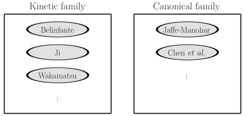
Figure 2: The Wakamatsu classification of proton spin decompositions into two families. See text for more details.

The potential angular momentum is itself a gauge-invariant quantity. Therefore, the splitting of the gauge potential into pure-gauge and physical terms allows one to decompose the proton spin into five gauge-invariant contributions, instead of the expected four. Based on this observation, Leader Leader:2011za criticized Wakamatsu’s classification arguing that one could in fact consider an infinite number of families by attributing a fraction $\alpha$ of the potential term to the electrons and the remaining fraction $(1-\alpha)$ to the photons. Note however that only the values $\alpha=0,1$ are natural as they simply correspond to the kinetic and canonical OAM, respectively. Leader favors the canonical version because the operators, at least at equal time, generate the expected rotations of the relevant fields, and this seems a reasonable property to demand for an angular momentum operator.

There is no totally convincing answer as to which family should be preferred. Deciding which family is the “physical” one appears to be essentially a matter of taste. This is somehow analogous to the scheme dependence in parton distribution functions, where it has been understood for some time that it is meaningless to claim that one has measured a quark distribution $q(x)$, but must specify which scheme e.g. $\overline{MS}$ or $DIS$ has been used. As long as one indicates clearly which version of the angular momentum one is using, it is irrelevant which one chooses.

IV.2 The covariant form of the decompositions

The Chen et al. split raised some concerns about the Lorentz symmetry as the definition of the pure-gauge and physical terms given in Eq. (148) does not look Lorentz covariant. More precisely, the question is: does the split of the Lorentz-transformed gauge potential coincide with the Lorentz transform of the split?

$$\begin{split}(\bm{A}^{\prime})_{\text{pure}}&\stackrel{{\scriptstyle?}}{{=}}(\bm{A}_{\text{pure}})^{\prime},\\ (\bm{A}^{\prime})_{\text{phys}}&\stackrel{{\scriptstyle?}}{{=}}(\bm{A}_{\text{phys}})^{\prime},\end{split}$$ (166)

where the prime indicates that the field is Lorentz transformed. To address this question, Wakamatsu developed a covariant version of the Chen et al. decomposition Wakamatsu:2010cb .

The starting point is the split of the four-component gluon potential into pure-gauge and physical terms

$$A_{\mu}(x)=A^{\text{pure}}_{\mu}(x)+A^{\text{phys}}_{\mu}(x).$$ (167)

This is simply the covariant version of the split of the gauge potential proposed by Chen et al. Chen:2008ag . As noticed in Ref. Lorce:2013gxa , this approach is not new, since it had already been adopted in 1962 by Schwinger Schwinger:1962zz ; Schwinger:1962fg and followed by Arnowitt and Fickler Arnowitt:1962cv . Moreover, the same idea reappeared in the works of e.g. Goto Goto:1966 , Treat Treat:1973yc ; Treat:1975dz , Duan Duan:1979 ; Duan:1984cb ; Duan:1998um ; Duan:2002vh , Fulp Fulp:1983bt , and Kashiwa and Tanimura Kashiwa:1996rs ; Kashiwa:1996hp . However, since Chen et al. revived this idea in the context of the controversy about the angular momentum decomposition, we shall refer to the generic split (167) as the “Chen et al. approach”.

By definition, the pure-gauge field is unphysical and therefore cannot contribute to the field-strength tensor

$$F^{\text{pure}}_{\mu\nu}=\partial_{\mu}A^{\text{pure}}_{\nu}-\partial_{\nu}A^{\text{pure}}_{\mu}=0.$$ (168)

Moreover, it is assumed to have the same gauge transformation law as the original gauge potential

$$A_{\mu}^{\text{pure}}(x)\mapsto\tilde{A}_{\mu}^{\text{pure}}(x)=A_{\mu}^{\text{pure}}(x)+\partial_{\mu}\alpha(x).$$ (169)

Note that the precise definition of the physical field is postponed until a later stage. Nonetheless the conditions (167)-(169) are actually sufficient for achieving a gauge-invariant decomposition of the angular momentum. The defining constraint (168) implies that the pure-gauge field can be put it the form

$$A_{\mu}^{\text{pure}}(x)=\partial_{\mu}\alpha_{\text{pure}}(x),$$ (170)

where $\alpha_{\text{pure}}(x)$ is some scalar function of spacetime. From Eq. (169), one easily derives the gauge transformation laws of the scalar and the physical fields

$$\begin{split}\alpha_{\text{pure}}(x)&\mapsto\tilde{\alpha}_{\text{pure}}(x)=\alpha_{\text{pure}}(x)+\alpha(x),\\ A_{\mu}^{\text{phys}}(x)&\mapsto\tilde{A}_{\mu}^{\text{phys}}(x)=A_{\mu}^{\text{phys}}(x).\end{split}$$ (171)

Note, in particular, that the physical field in QED is gauge invariant, just like the field-strength tensor. Because of Eq. (168), the latter can simply be expressed as

$$F_{\mu\nu}=\partial_{\mu}A^{\text{phys}}_{\nu}-\partial_{\nu}A^{\text{phys}}_{\mu}.$$ (172)

IV.2.1 The gauge-invariant canonical decomposition

The Wakamatsu covariant generalization of the Chen et al. decomposition will be referred to as the gauge-invariant canonical (gic) decomposition. It reads at the density level Wakamatsu:2010cb

$$M^{\mu\nu\rho}=S^{\mu\nu\rho}_{\text{gic},e}+L^{\mu\nu\rho}_{\text{gic},e}+S^{\mu\nu\rho}_{\text{gic},\gamma}+L^{\mu\nu\rho}_{\text{gic},\gamma}+M^{\mu\nu\rho}_{\text{gic},\text{boost}}+\text{four-divergence},$$ (173)

where the electron spin, electron OAM, photon spin, and photon OAM densities are given by

$$\begin{split}S^{\mu\nu\rho}_{\text{gic},e}&=\tfrac{1}{2}\,\epsilon^{\mu\nu\rho\sigma}\overline{\psi}\gamma_{\sigma}\gamma_{5}\psi,\\ L^{\mu\nu\rho}_{\text{gic},e}&=\overline{\psi}\gamma^{\mu}x^{[\nu}iD^{\rho]}_{\text{pure}}\psi,\\ S^{\mu\nu\rho}_{\text{gic},\gamma}&=-F^{\mu[\nu}A^{\rho]}_{\text{phys}},\\ L^{\mu\nu\rho}_{\text{gic},\gamma}&=-F^{\mu\alpha}x^{[\nu}\partial^{\rho]}A^{\text{phys}}_{\alpha},\end{split}$$ (174)

with $D^{\text{pure}}_{\mu}=\partial_{\mu}+ieA^{\text{pure}}_{\mu}$ the pure-gauge covariant derivative, and $\epsilon^{\mu\nu\rho\sigma}$ the totally antisymmetric Levi-Civita tensor satisfying $\epsilon_{0123}=+1$. We do not need to write down explicitly the boost term, because it does not contribute to the angular momentum expressions $M^{0ij}_{\text{gic},\text{boost}}=0$. We also do not need to write down explicitly the four-divergence term as it corresponds, once integrated over spatial coordinates, to a surface term assumed to vanish. The complete expressions for a generic gauge theory will however be given in section V.

This decomposition is clearly gauge invariant and has a strong resemblance with the covariant form of the Jaffe-Manohar decomposition. Indeed, starting from the gauge-invariant canonical decomposition, one can choose to work in the gauge where $A_{\mu}^{\text{pure}}=0$, obtained with the gauge transformation function $\alpha(x)=-\alpha_{\text{pure}}(x)$. In that gauge, one has $A_{\mu}=A^{\text{phys}}_{\mu}$ and $D^{\text{pure}}_{\mu}=\partial_{\mu}$, so that the gauge-invariant canonical decomposition takes the same mathematical form as the Jaffe-Manohar decomposition

$$\begin{split}S^{\mu\nu\rho}_{\text{gic},e}\big{|}_{A^{\text{pure}}_{\mu}=0}&=S^{\mu\nu\rho}_{\text{JM},e},\\ L^{\mu\nu\rho}_{\text{gic},e}\big{|}_{A^{\text{pure}}_{\mu}=0}&=L^{\mu\nu\rho}_{\text{JM},e},\\ S^{\mu\nu\rho}_{\text{gic},\gamma}\big{|}_{A^{\text{pure}}_{\mu}=0}&=S^{\mu\nu\rho}_{\text{JM},\gamma},\\ L^{\mu\nu\rho}_{\text{gic},\gamma}\big{|}_{A^{\text{pure}}_{\mu}=0}&=L^{\mu\nu\rho}_{\text{JM},\gamma}.\end{split}$$ (175)

The gauge-invariant canonical decomposition can then be thought of as a gauge-invariant extension (GIE) of the Jaffe-Manohar decomposition Hoodbhoy:1998bt ; Ji:2012gc . However, as stressed e.g. by Hatta, in this scheme there is no actual definition given for the field $A^{\mu}_{\text{phys}}$. The issue of the freedom in choosing $A^{\mu}_{\text{phys}}$ will be discussed in the next section. The concept of GIE can be applied to any gauge non-invariant quantity like e.g. the Chern-Simons current Guo:2012wv . It consists in finding a gauge-invariant quantity that gives the same physical results as a gauge non-invariant quantity evaluated in a specific gauge Hoodbhoy:1998bt ; Ji:2012gc .

IV.2.2 The gauge-invariant kinetic decomposition

Wakamatsu also proposed a second type of gauge-invariant covariant decomposition, which will be referred to as the gauge-invariant kinetic (gik) decomposition, and is simply related to the gauge-invariant canonical decomposition as follows Wakamatsu:2010cb

$$\begin{split}S^{\mu\nu\rho}_{\text{gik},e}&=S^{\mu\nu\rho}_{\text{gic},e},\\ L^{\mu\nu\rho}_{\text{gik},e}&=L^{\mu\nu\rho}_{\text{gic},e}-L^{\mu\nu\rho}_{\text{pot}},\\ S^{\mu\nu\rho}_{\text{gik},\gamma}&=S^{\mu\nu\rho}_{\text{gic},\gamma},\\ L^{\mu\nu\rho}_{\text{gik},\gamma}&=L^{\mu\nu\rho}_{\text{gic},\gamma}+L^{\mu\nu\rho}_{\text{pot}},\end{split}$$ (176)

where, following Konopinski’s terminology Konopinski , the covariant potential angular momentum is given by

$$\begin{split}L^{\mu\nu\rho}_{\text{pot}}&=e\overline{\psi}\gamma^{\mu}\psi\,x^{[\nu}A_{\text{phys}}^{\rho]}\\ &=(\partial_{\alpha}F^{\alpha\mu})\,x^{[\nu}A^{\rho]}_{\text{phys}}.\end{split}$$ (177)

Note that the QED equation of motion $\partial_{\alpha}F^{\alpha\mu}=e\overline{\psi}\gamma^{\mu}\psi$ has been used in order to be able to write the potential angular momentum as either an electron or a photon contribution. The sum of the photon spin and OAM appearing in the gauge-invariant kinetic decomposition coincides (up to a four-divergence term) with the photon total angular momentum appearing in the covariant form of the Ji decomposition

$$\begin{split}S^{\mu\nu\rho}_{\text{Ji},e}&=S^{\mu\nu\rho}_{\text{gik},e},\\ L^{\mu\nu\rho}_{\text{Ji},e}&=L^{\mu\nu\rho}_{\text{gik},e},\\ J^{\mu\nu\rho}_{\text{Ji},\gamma}&=S^{\mu\nu\rho}_{\text{gik},\gamma}+L^{\mu\nu\rho}_{\text{gik},\gamma}+\text{four-divergence}.\end{split}$$ (178)

Moreover, following Lorcé’s observation Lorce:2013fpa , we note that the gauge-invariant kinetic photon OAM can alternatively be written as

$$L^{\mu\nu\rho}_{\text{gik},\gamma}=x^{\nu}\left(A^{\rho}_{\text{phys}}\partial_{\lambda}-A^{\text{phys}}_{\lambda}\partial^{\rho}\right)F^{\lambda\mu}-(\nu\leftrightarrow\rho)+\text{four-divergence},$$ (179)

where one recognizes the gauge-invariant kinetic photon momentum

$$T^{\mu\rho}_{\text{gik},\gamma}=F^{\mu\lambda}F_{\lambda}^{\phantom{\alpha}\rho}=\left(A^{\rho}_{\text{phys}}\partial_{\lambda}-A^{\text{phys}}_{\lambda}\partial^{\rho}\right)F^{\lambda\mu}+\text{four-divergence},$$ (180)

where we have used Eq. (172) and ignored the term $g^{\mu\rho}\,\tfrac{1}{4}F^{\alpha\beta}F_{\alpha\beta}$, because it does not contribute to the momentum expressions obtained with $\mu=0$ and $\rho=i$. Complete expressions for a general gauge theory will be given in the next section.

IV.3 The ambiguity in defining $A^{\text{phys}}_{\mu}$

Let us pause for a moment and discuss a new issue raised by the Wakamatsu covariant form. While the conditions (168) and (169) on the pure-gauge term are sufficient to construct complete gauge-invariant decompositions of the angular momentum in a seemingly covariant form, it is actually not sufficient to determine the precise form of $A^{\text{pure}}_{\mu}$ and $A^{\text{phys}}_{\mu}$. As observed by Stoilov Stoilov:2010pv and discussed in more detail by Lorcé Lorce:2012rr ; Lorce:2012ce , the split of the gauge potential into pure-gauge and physical terms introduces a new symmetry.

IV.3.1 The Stueckelberg symmetry

For a given split into pure-gauge and physical terms $A_{\mu}=A^{\text{pure}}_{\mu}+A^{\text{phys}}_{\mu}$, it is always possible to define a new split $A_{\mu}=\bar{A}^{\text{pure}}_{\mu}+\bar{A}^{\text{phys}}_{\mu}$ where

$$\begin{split}\bar{A}^{\text{pure}}_{\mu}(x)&=A^{\text{pure}}_{\mu}(x)+\partial_{\mu}C(x),\\ \bar{A}^{\text{phys}}_{\mu}(x)&=A^{\text{phys}}_{\mu}(x)-\partial_{\mu}C(x)\end{split}$$ (181)

with $C(x)$ an arbitrary scalar function of spacetime. Notice that this is not a gauge transformation since $\bar{A}_{\mu}=A_{\mu}$. The new pure-gauge term $\bar{A}^{\text{pure}}_{\mu}$ automatically satisfies the condition (168)

$$F^{\text{pure}}_{\mu\nu}=0\qquad\Rightarrow\qquad\bar{F}^{\text{pure}}_{\mu\nu}=0,$$ (182)

and also the gauge transformation law (169), provided that $C(x)$ is gauge invariant.

So, if one starts with a gauge-invariant Lagrangian involving only the full gauge potential $A_{\mu}$, this Lagrangian will automatically be invariant under the new transformation (181). Because of the similarity with the famous Stueckelberg mechanism, this symmetry is referred to as the Stueckelberg symmetry. The Stueckelberg symmetry group turns out to be a simple copy of the gauge symmetry group, though acting in a different manner on the fields. Just like the QED Lagrangian, the Belinfante and Ji decompositions involve only the full gauge potential, and so are automatically invariant under Stueckelberg transformations. On the contrary, the gauge-invariant canonical and kinetic decompositions rely on our ability to separate the gauge potential into pure-gauge and physical terms. While gauge invariant by construction, these decompositions are obviously not Stueckelberg invariant. This means that for different explicit definitions of $A^{\text{phys}}_{\mu}$, different physical values will be attributed to the electron and photon contributions. For a schematic view, see Fig. 3.

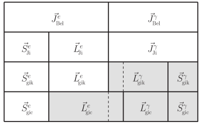
Figure 3: A schematic view of the Belinfante, Ji, gauge-invariant kinetic and gauge-invariant canonical decompositions. In white are depicted the pieces that are Stueckelberg invariant, and in gray are depicted the pieces that are Stueckelberg non-invariant. The potential OAM corresponds to the piece delimited by a dashed line common to both $\bm{L}^{e}_{\text{gic}}$ and $\bm{L}^{\gamma}_{\text{gik}}$.

IV.3.2 Towards a more refined classification

Since the gauge-invariant canonical and kinetic decompositions are Stueckelberg non-invariant, they should rather be seen as representing two different classes of decompositions. There are in principle infinitely many possible gauge-invariant canonical and kinetic decompositions, differing in the way one explicitly splits the gauge potential into pure-gauge and physical contributions. In order to single out a particular element in a class, one has to impose an additional constraint on the physical field that fixes the Stueckelberg symmetry. Note that it is necessary to impose a constraint that does not look Lorentz covariant to get completely rid of the Stueckelberg symmetry. Indeed, any explicitly covariant condition, like e.g. the Lorenz constraint $\partial_{\mu}A^{\mu}_{\text{phys}}=0$ Cho:2010cw ; Cho:2011ee ; Guo:2012wv ; Guo:2013jia or the Fock-Schwinger constraint $x_{\mu}A_{\text{phys}}^{\mu}=0$, leaves some residual Stueckelberg symmetry Zhang:2011rn . In order to specify a unique decomposition, this residual symmetry must also be fixed. The fixing of the Stueckelberg symmetry simply mirrors the fixing of the gauge symmetry, and so all the difficulties encountered with the latter have a counterpart with the former.

In the Chen et al. and Wakamatsu decompositions, the physical field was defined by the Coulomb constraint $\bm{\nabla}\cdot\bm{A}_{\text{phys}}=0$. These decompositions therefore simply correspond to the Coulomb gauge-invariant canonical and gauge-invariant kinetic decompositions, respectively. This choice was motivated by the desire to recover the well-known Helmholtz decomposition in QED of the vector potential into longitudinal $\bm{A}_{\text{pure}}=\bm{A}_{\parallel}$ and transverse $\bm{A}_{\text{phys}}=\bm{A}_{\perp}$ parts, which is unique once the Lorentz frame is fixed Jauch:1955jr ; Berestetskii ; Cohen . However, it is perfectly legitimate to impose a different constraint. For example, with the motivation of making contact with the parton model of QCD, Hatta imposed the light-front constraint $A^{+}_{\text{phys}}=0$ with additional boundary conditions at infinity Hatta:2011ku ; Lorce:2012ce . The decomposition he obtained corresponds to the light-front gauge-invariant canonical decomposition. A schematic picture of the refined classification is illustrated in Fig. 4.

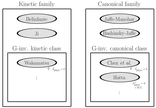
Figure 4: Refinement of the Wakamatsu classification depicted in Fig. 2. See text for more details.

Except for Wakamatsu, there is a general agreement about the fact that different elements in a same class will generally lead to different physical results, i.e. give different numerical answers for the expectation values of the operators involved. One should be careful not to confuse a gauge fixing with a Stueckelberg fixing. For example, in the covariant form of the Chen et al. decomposition, we can generalise their three-dimenisonal constraints by demanding that the pure-gauge field vanishes only in the Coulomb gauge [for the explicit form of $A^{\text{pure}}_{\mu}$ and $A^{\text{phys}}_{\mu}$, see Eq. (189)]

$$A^{\mu,\text{Chen}}_{\text{pure}}\big{|}_{\bm{\nabla}\cdot\bm{A}=0}=0,\qquad A^{\mu,\text{Chen}}_{\text{pure}}\big{|}_{A^{+}=0\,+\,\text{B.C.}}\neq 0,$$ (183)

while in the Hatta decomposition, the pure-gauge field vanishes only in the light-front gauge with appropriate boundary conditions

$$A^{\mu,\text{Hatta}}_{\text{pure}}\big{|}_{\bm{\nabla}\cdot\bm{A}=0}\neq 0,\qquad A^{\mu,\text{Hatta}}_{\text{pure}}\big{|}_{A^{+}=0\,+\,\text{B.C.}}=0.$$ (184)

Explicit expressions for $A_{\mu}^{\text{pure}}$ and $A_{\mu}^{\text{phys}}$ in both Chen et al. and Hatta decompositions are given in the next subsection. Even though the Chen et al. and Hatta decompositions share the same abstract mathematical structure in terms of $A^{\text{pure}}_{\mu}$ and $A^{\text{phys}}_{\mu}$, they generally lead to different physical results. Indeed, the Chen et al. decomposition coincides with the Jaffe-Manohar decomposition in the Coulomb gauge. In the light-front gauge, the Hatta decomposition reduces to the Bashinsky-Jaffe decomposition Bashinsky:1998if , which is a residual GIE of the Jaffe-Manohar decomposition Wakamatsu:2010cb ; Lorce:2012ce . Only when imposing further boundary conditions does the Hatta decomposition reduce to the Jaffe-Manohar decomposition itself. These relations are schematically represented in Fig. 5. Since the Jaffe-Manohar decomposition is not gauge invariant, it is expected to give different results in the Coulomb gauge and in the light-front gauge with some boundary conditions, see Fig. 6 for an illustration. It then follows that different gauge-invariant canonical decompositions, i.e. GIEs of the Jaffe-Manohar decomposition based on different constraints, are generally not physically equivalent. Wakamatsu’s discussions about the relation between the gauge-invariant canonical decomposition, the Chen et al. decomposition and the Jaffe-Manohar decomposition in the light-front gauge is rather confusing, as there is no clear distinction between the gauge-fixing procedure and the Stueckelberg-fixing procedure Wakamatsu:2010cb ; Wakamatsu:2012ve . It is because of this that he wrongly concluded that all the GIEs are physically equivalent.

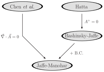
Figure 5: Relations between the Chen et al., Hatta, Bashinsky-Jaffe and Jaffe-Manohar decompositions. The Chen et al. decomposition reduces to the Jaffe-Manohar decomposition in the Coulomb gauge. The Hatta decomposition reduces to the Bashinsky-Jaffe decomposition in the light-front gauge and reduces further to the Jaffe-Manohar decomposition once appropriate boundary conditions are imposed on the gauge potential.

Figure 6: Schematic visualization of the effect of gauge fixing (vertical lines) and Stueckelberg fixing (horizontal lines). While the gauge non-invariant operators $\hat{O}_{\text{JM}}$ belonging to the Jaffe-Manohar decomposition lead to different physical results in different gauges (dotted line), the operators $\hat{O}_{\text{Chen}}$ and $\hat{O}_{\text{Hatta}}$ belonging, respectively, to the Coulomb and light-front GIEs are gauge invariant (dashed lines). Since one has $\hat{O}_{\text{Chen}}=\hat{O}_{\text{JM}}$ in the Coulomb gauge and $\hat{O}_{\text{Hatta}}=\hat{O}_{\text{JM}}$ in the light-front gauge with appropriate boundary conditions, different GIEs of the same gauge non-invariant quantity are physically inequivalent $\langle\hat{O}_{\text{Chen}}\rangle\neq\langle\hat{O}_{\text{Hatta}}\rangle$.

We would like to stress here the similarities with the more familiar procedure of Lorentz-invariant extension (LIE). In relativity, the mass $m$ of a particle is not frame independent. It is given by $m=\gamma m_{0}$, where $m_{0}$ is the inertial mass in the rest frame and $\gamma=1/\sqrt{1-v^{2}}$ is the boost factor with $v$ the velocity of the particle in units of the speed of light. One can consider the Lorentz-invariant quantity $p^{2}=E^{2}-\bm{p}^{2}$ as a LIE of the quantity $m^{2}$, which agrees with the value of $m^{2}$ in the rest frame, i.e. in the frame where $m=m_{0}$. Similarly, the Mandelstam variable $s$ is the LIE of the square of the center-of-mass energy $E^{2}_{\text{CM}}$.

Strictly speaking, one does not measure the rest mass of particles produced in high-energy experiments, because these particles are usually far from being at rest. What is actually measured is the LIE $p^{2}$ which can be interpreted in the rest frame as the square of the particle inertial mass. It is in this sense that one has to understand the “measurement” of a particle rest mass. Similarly, a gauge non-invariant quantity is strictly speaking not measurable. However, it is possible to measure its GIE, i.e. a gauge-invariant quantity which coincides in a certain fixed gauge with the gauge non-invariant quantity Hoodbhoy:1998bt ; Ji:2012gc . For example, even if the Jaffe-Manohar decomposition is gauge non-invariant, it is considered to be “measurable” in the light-front gauge Jaffe:1989jz . This is justified by the fact that what is actually measurable is the Hatta decomposition, which is its light-front GIE.

IV.3.3 Origin and geometrical interpretation of the Stueckelberg symmetry

Even though formally gauge invariant, the Chen et al. approach gives a special or privileged role to some gauge. It is the gauge where the full gauge potential satisfies the same constraint as the physical gauge potential, i.e. the gauge where $A^{\text{pure}}_{\mu}=0$. For example, in the Chen et al. and Wakamatsu three-dimensional decompositions, this special gauge is simply the Coulomb gauge $\bm{\nabla}\cdot\bm{A}=0$, since the physical field was defined by the Coulomb constraint $\bm{\nabla}\cdot\bm{A}_{\text{phys}}=0$. In the Hatta decomposition, it is the light-front gauge $A^{+}=0$ with advanced, retarded or antisymmetric boundary conditions. The fact that there exists a preferred or natural gauge in the Chen et al. approach seems at odds with the spirit of gauge symmetry, in the sense that all the gauges should in principle be physically equivalent. Moreover, since writing a GIE consists in finding the gauge-invariant operator which leads to the same physical results as a gauge non-invariant operator in some fixed gauge, determining a specific GIE is somehow equivalent to fixing a gauge for the gauge non-invariant quantity. It appears therefore that gauge symmetry and Stueckelberg symmetry are tightly connected. Our purpose here is to reveal the geometrical meaning of the Stueckelberg symmetry and its relation with gauge symmetry.

In order to better understand the origin and the physical meaning of the Stueckelberg symmetry, it is useful to consider first some explicit example. As shown explicitly by Hatta with the light-front GIE of the Jaffe-Manohar decomposition Hatta:2011ku and generalized later by Lorcé Lorce:2012ce , the Chen et al. approach amounts in many cases to adding Wilson lines along some path to preserve the gauge symmetry. The presence of a Wilson line clearly indicates that explicit expressions for $A^{\text{pure}}_{\mu}$ and $A^{\text{phys}}_{\mu}$ in terms of $A_{\mu}$ are usually non-local and path dependent. The freedom in the choice of the path appears to be at the origin of the Stueckelberg symmetry. Namely, Stueckelberg-invariant quantities are path independent, whereas path-dependent quantities are Stueckelberg non-invariant. A choice of path automatically renders one gauge special, namely the gauge where the Wilson line factor reduces to unity. For a generic path, this particular gauge is known as the contour gauge Ivanov:1985np . For example, the Wilson lines in the light-front GIE run along the light-front direction $n^{\mu}=\tfrac{1}{\sqrt{2}}\,(1,0,0,-1)$

$$\mathcal{W}_{\text{LF}}(x,\pm\infty)=e^{-ie\int^{0}_{\pm\infty}A^{+}(x+\lambda n)\,\mathrm{d}\lambda},$$ (185)

and reduce to unity in the light-front gauge $A^{+}=n\cdot A=0$. The pure-gauge and physical fields in the Hatta decomposition can then be written in an explicitly non-local form

$$\begin{split}A^{\mu,\text{Hatta}}_{\text{pure}}(x)&=-\frac{i}{e}\,\mathcal{W}_{\text{LF}}(x,\pm\infty)\partial^{\mu}\mathcal{W}_{\text{LF}}(\pm\infty,x)=\int^{0}_{\pm\infty}\partial^{\mu}A^{+}(x+\lambda n)\,\mathrm{d}\lambda,\\ A^{\mu,\text{Hatta}}_{\text{phys}}(x)&=A^{\mu}(\pm\infty)+\int^{0}_{\pm\infty}F^{+\mu}(x+\lambda n)\,\mathrm{d}\lambda,\end{split}$$ (186)

where $A^{+}(\pm\infty)=0$. In particular, one has

in any gauge $$A^{+,\text{Hatta}}_{\text{pure}}(x) =A^{+}(x), A^{+,\text{Hatta}}_{\text{phys}}(x)=0,$$ (187)

in the light-front gauge $$A^{\mu,\text{Hatta}}_{\text{pure}}(x) =0, A^{\mu,\text{Hatta}}_{\text{phys}}(x)=A^{\mu}(x).$$ (188)

To keep the example simple, we have not included the transverse gauge links at spatial light-front infinity $x^{-}=\pm\infty$. A more detailed discussion including these contributions can be found in Ref. Lorce:2012ce .

The Stueckelberg dependence is actually more general than the path dependence, since some GIEs, like e.g. the Coulomb GIE or the Lorenz GIE, cannot be written simply in terms of Wilson lines, and are in this sense path independent Belinfante:1962zz ; Mandelstam:1962mi ; Rohrlich:1965 ; Yang:1985 ; Kashiwa:1994jn ; Kashiwa:1997we . The explicit expressions for $A^{\text{pure}}_{\mu}$ and $A^{\text{phys}}_{\mu}$ in terms of $A_{\mu}$ in these path-independent GIEs are nevertheless again non-local Zhang:2011rn . For example, in the Chen et al. decomposition (and therefore also in the Wakamatsu decomposition), the pure-gauge and physical fields explicitly read

$$\begin{split}A^{\mu,\text{Chen}}_{\text{pure}}(x)&=-\partial^{\mu}\frac{1}{\bm{\nabla}^{2}}\bm{\nabla}\cdot\bm{A}(x),\\ A^{\mu,\text{Chen}}_{\text{phys}}(x)&=-\frac{1}{\bm{\nabla}^{2}}\partial_{i}F^{i\mu}(x),\end{split}$$ (189)

where the non-local expressions arise owing to the inverse Laplace operator, see Eq. (158). In particular, one has

in any gauge $$\bm{\nabla}\cdot\bm{A}^{\text{Chen}}_{\text{pure}}(x) =\bm{\nabla}\cdot\bm{A}(x), \bm{\nabla}\cdot\bm{A}^{\text{Chen}}_{\text{phys}}(x)=0,$$ (190)

in the Coulomb gauge $$A^{\mu,\text{Chen}}_{\text{pure}}(x) =0, A^{\mu,\text{Chen}}_{\text{phys}}(x)=A^{\mu}(x).$$ (191)

Gauge-invariant, Stueckelberg non-invariant quantities are therefore intrinsically non-local, i.e. cannot be written as gauge-invariant local expressions in terms of the full gauge potential $A_{\mu}$. On the contrary, quantities that are both gauge and Stueckelberg invariant can in principle be written as gauge-invariant local expressions in terms of $A_{\mu}$. Non-local expressions are often considered to be dangerous, because they may lead to violations of causality. Note however that unphysical pure-gauge degrees of freedom are allowed to propagate faster than light since they are decoupled from the physical observables. In the Chen et al. approach, one can always work in the gauge where $A^{\text{pure}}_{\mu}(x)=0$ so that $A^{\text{phys}}_{\mu}(x)=A_{\mu}(x)$. This means that there always exists a gauge where the Stueckelberg non-invariant expressions reduce to a local form in terms of $A_{\mu}$. No genuine violation of causality is therefore expected in the Chen et al. approach.

In some sense, the Chen et al. approach can be seen as a convenient rewriting of complicated non-local expressions (RHS of Eqs. (186) and (189)) in terms of simpler seemingly local expressions (LHS of Eqs. (186) and (189)). This means that, contrary to what they claim, Chen et al. Chen:2008ag do not really contradict the textbook statement that there exist no gauge-invariant local operators for the photon spin and OAM Cohen ; Simmons . Alternatively, one could say that the Chen et al. approach allows one to get around the textbook statement by considering two four-vector fields at one point, $A^{\text{pure}}_{\mu}(x)$ and $A^{\text{phys}}_{\mu}(x)$, instead of a single one, $A_{\mu}(x)$.

We have seen that Stueckelberg symmetry is related to the ability to write local expressions in terms of the full gauge potential. Lorcé showed that Stueckelberg symmetry can also be understood from a different point of view, closer to the discussions in General Relativity and String Theory Lorce:2013bja . He also observed that the Chen et al. approach is pretty similar to the background field method introduced by DeWitt DeWitt:1967ub ; DeWitt:1967uc ; DeWitt:1980jv ; 'tHooft:1975vy ; Grisaru:1975ei ; Boulware:1980av ; Abbott:1980hw , which has been extensively used in gravity and supergravity 'tHooft:1973us ; 'tHooft:1974bx ; Deser:1977nt ; Abbott:1981ff ; Petrov:2007xva ; Petrov:2012qn , as well as in both continuum and lattice gauge theories Dashen:1980vm ; Abbott:1982jh ; Luscher:1995vs ; Freire:2000bq ; Binosi:2009qm ; Binosi:2012st . A nice introduction to the background field method has been provided by Abbott in Ref. Abbott:1981ke .

When discussing gauge transformations, one usually does not specify whether these are considered as active transformations (i.e. the system is modified) or passive transformations (i.e. the reference axes are modified) Guay:2004zz . The reason for this is that there is usually no way to distinguish active gauge transformations from passive gauge transformations. As a matter of fact, physicists tend to think of gauge transformations as passive transformations, and therefore consider that gauge symmetry is just a mere redundancy of the mathematical description. On the contrary, mathematicians think of gauge transformations as active transformations, and so consider that gauge symmetry is a physical property of the system.

The situation changes however once one introduces some background field in the theory DeWitt:1967ub ; Abbott:1981ke , as the latter transforms differently under active and passive transformations Smolin:2005mq ; Rickles:2008 ; Rozali:2008ex ; Barenz:2012av . In the Chen et al. approach, it is the pure-gauge field $A^{\text{pure}}_{\mu}(x)$ that plays the role of a non-dynamical, background field Zhang:2011rn ; Lorce:2013gxa ; Lorce:2013bja . Stueckelberg dependence is therefore simply equivalent to background dependence. Notice that, from the gauge transformation law of the electron field, it is not possible to derive the gauge transformation law for the pure-gauge and physical fields, separately. This is the reason why, in the covariant version of the Chen et al. approach, it is assumed that the pure-gauge field transforms in the same way as the full gauge potential. This assumption corresponds actually to passive gauge transformations, as the latter consist in a mere change of coordinates, which affects in the same way dynamical and background fields. On the contrary, under active gauge transformations, the dynamical and background fields are transformed in a different way Rickles:2008 ; Barenz:2012av ; Lorce:2013bja .

Table 1: The expressions for the different fields after passive gauge transformations, active gauge transformations and Stueckelberg transformations. The interesting case is $C(x)=-\beta(x)=\alpha(x)$.

Fields	Passive gauge	Active gauge	Stueckelberg
$\psi(x)$	$e^{-ie\alpha(x)}\psi(x)$	$e^{-ie\beta(x)}\psi(x)$	$\psi(x)$
$A_{\mu}(x)$	$A_{\mu}(x)+\partial_{\mu}\alpha(x)$	$A_{\mu}(x)+\partial_{\mu}\beta(x)$	$A_{\mu}(x)$
$A^{\text{pure}}_{\mu}(x)$	$A^{\text{pure}}_{\mu}(x)+\partial_{\mu}\alpha(x)$	$A^{\text{pure}}_{\mu}(x)$	$A^{\text{pure}}_{\mu}(x)+\partial_{\mu}C(x)$
$A^{\text{phys}}_{\mu}(x)$	$A^{\text{phys}}_{\mu}(x)$	$A^{\text{phys}}_{\mu}(x)+\partial_{\mu}\beta(x)$	$A^{\text{phys}}_{\mu}(x)-\partial_{\mu}C(x)$

In Table 1, we compare the expressions for the transformed fields under passive gauge transformations, active gauge transformations and Stueckelberg transformations. Using $C(x)=-\beta(x)=\alpha(x)$, it appears that the Stueckelberg transformations simply correspond to passive gauge transformations followed by the corresponding inverse active gauge transformations Lorce:2013bja . In particular, one can now easily understand why the Stueckelberg symmetry group is a simple copy of the gauge symmetry group. The set of passive and active gauge transformations (second and third columns of Table 1) is therefore equivalent to the set of (passive) gauge and Stueckelberg transformations (second and fourth columns of Table 1). Since most of the recent papers on the proton spin decomposition deal with the second set, we adopt it also in our subsequent discussions. Therefore, unless explicitly stated, the gauge transformations in the following always refer to the passive ones (second column of Table 1).

IV.3.4 Measurability and the controversy about Stueckelberg symmetry

Ji criticized the Chen et al. approach arguing that their notion of gauge invariance does not coincide with the “usual textbook type” Ji:2009fu ; Ji:2010zza , where physical observables are usually constructed from gauge-invariant local operators. Moreover, having stressed that the Chen et al. decomposition simply corresponds to the Coulomb GIE of the Jaffe-Manohar decomposition, Ji, Xu and Zhao wrote in Ref. Ji:2012gc that “the GIE of an intrinsically gauge-noninvariant quantity is not naturally gauge invariant” and that “GIE operators are in general unmeasurable. So far, the only example is offered in high-energy scattering in which certain partonic GIE operators may be measured.” This kind of statement is pretty confusing as it seems at first sight self-contradictory. Indeed, how can a measurable quantity be “not naturally gauge invariant” or, using Wakamatsu’s words Wakamatsu:2013voa , “not a gauge-invariant quantity in a true or traditional sense”?

This aspect of the controversy can easily be clarified by using a more precise terminology. Indeed, the discussions in the previous subsection suggest the importance of distinguishing two forms of gauge invariance, weak and strong Lorce:2013bja :

• Weak gauge symmetry refers to the invariance under gauge transformations only. Intrinsically non-local (i.e. Stueckelberg non-invariant) expressions are allowed as long as they are gauge invariant;

• Strong gauge symmetry refers to the invariance under both gauge and Stueckelberg transformations. In other words, only the gauge-invariant expressions that can be written locally in terms of $A_{\mu}$ are allowed.

Clearly, when Ji invokes the usual textbook gauge invariance, he refers to the strong form of gauge symmetry, and the claim that “the GIE of an intrinsically gauge-noninvariant quantity is not naturally gauge invariant” should be understood as “a Stueckelberg non-invariant GIE is gauge invariant in a weak sense only”. Wakamatsu appears to be less restrictive. Indeed, he writes in Ref. Wakamatsu:2013voa that “if a quantity in question is seemingly gauge-invariant but path-dependent, it is not a gauge-invariant quantity in a true or traditional sense, which in turn indicates that it may not correspond to genuine observable.” This is motivated by the claim in Refs. Belinfante:1962zz ; Mandelstam:1962mi ; Rohrlich:1965 ; Yang:1985 that path dependence is a reflection of gauge dependence. He therefore considers that physical quantities may be intrinsically non-local, provided that they are path independent. Wakamatsu therefore requires something that is in between the weak and strong forms of gauge symmetry. Note however that, from the discussions in the previous subsection, it should be clear that path dependence is not gauge dependence, but rather some instance of Stueckelberg dependence. Otherwise, this would mean that all the parton high-energy physics, based on Wilson lines running along the light-front direction, is also not gauge invariant. This shows once more the importance of distinguishing gauge symmetry from Stueckelberg symmetry.

Now comes the essential question of measurability, which we think has been grossly misconstrued in the literature. Measurable quantities are quantities that can in principle be extracted from experimental data. It turns out that a sufficient condition for measurability is that an operator satisfies just the condition of the weak form of gauge invariance. For example, the parton distribution functions are defined as particular matrix elements of gauge-invariant non-local partonic operators. Such quantities can be extracted from experiments thanks to the so-called factorization theorems that allow one to approximate a cross section by a convolution of these (process-independent) parton distribution functions with a perturbatively calculable (process-dependent) partonic cross section Collins . We would also like to stress that many physical phenomena, like e.g. the Aharonov-Bohm effect, originate from a topological problem which cannot be addressed from a purely local point of view. This shows that the measurable quantities are not necessarily intrinsically local. Requiring strong form of gauge invariance to decide whether a quantity is measurable or not is therefore excessive. Put in different words, it is sufficient that a measurable operator is gauge invariant in the weak sense but, as we have seen, not necessarily “naturally gauge invariant” (i.e. gauge invariant in a strong sense). However this is far from being necessary. Collins Collins:1984xc has given explicit examples of gauge non-invariant operators whose expectation values are gauge independent. And Leader Leader:2011za has shown that, in covariantly quantized QED, even the total momentum and angular momentum, i.e. operators which have none of the problems linked to the separation into constituent contributions, are not gauge invariant, yet, crucially, their expectation values are gauge independent. The key point is that in a gauge theory, care has to be exercised in considering matrix elements only between physical states.

Following Lorcé’s suggestion Lorce:2013bja , measurable quantities that can be written locally in terms of $A_{\mu}$ (i.e. that are Stueckelberg invariant or gauge invariant in a strong sense) are called observables, while those that are intrinsically non-local (i.e. Stueckelberg non-invariant or gauge invariant in a weak sense) are called quasi-observables. While the Belinfante and Ji decompositions involve only observables, quasi-observables appear in the gauge-invariant canonical and gauge-invariant kinetic decompositions, see the gray contributions in Fig. 3. All these decompositions are in principle measurable, since they fulfill the requirement of weak gauge symmetry. This makes some people feel uncomfortable because, in some sense, there should be only one “truly physical” picture. However, these arguments are somewhat metaphysical. What counts in Physics should be measurability. From this point of view, there is no reason to disregard quasi-observables and not to consider the gauge-invariant canonical and gauge-invariant kinetic decompositions. In addition, this sort of argument about the properties of the operators completely ignores the point of view stressed by Collins Collins:1984xc and Leader Leader:2011za that what is finally relevant is whether the expectation value of an operator is or is not independent of the gauge choice. If it is gauge independent, then that is all that matters and it is in principle measurable. Unfortunately, it is difficult to see, apart from explicit calculations, whether or not a gauge non-invariant operator leads to gauge-independent matrix elements.

As mentioned previously, the Chen et al. approach is a typical example of a GIE. Considering any gauge non-invariant object in a specific gauge, one can easily construct a gauge-invariant object leading to the same physical result in any gauge. Formally, it is sufficient to replace the full gauge potential $A_{\mu}$ by the physical field $A^{\text{phys}}_{\mu}$, and the ordinary derivative $\partial_{\mu}$ by the appropriate pure-gauge covariant derivative. Starting from a single gauge non-invariant local quantity, one can construct infinitely many GIEs. There exist therefore formally infinitely many gauge-invariant canonical and gauge-invariant kinetic decompositions that are in principle measurable. According to Chen et al. Chen:2008ag ; Chen:2009mr and Wakamatsu Wakamatsu:2010cb ; Wakamatsu:2012ve ; Wakamatsu:2013voa , the Stueckelberg symmetry does not exist from the very beginning. They indeed claim that the Coulomb gauge $\bm{\nabla}\cdot\bm{A}=0$ is the “physical” gauge, since it is the one compatible with the Helmholtz decomposition. Wakamatsu further argues that the Coulomb constraint is the “physical” one because its explicit non-local expression in terms of the full gauge potential is path independent, contrary to other constraints like e.g. the light-front constraint Wakamatsu:2013voa . Accordingly, the GIE defined by the Coulomb constraint $\bm{\nabla}\cdot\bm{A}_{\text{phys}}=0$ is considered by them as the only “physical” one. We strongly disagree with such a statement. It is certainly true that, in electrodynamics, the Helmholtz decomposition appears particularly appealing. One should however keep in mind that there cannot be any experimental way to prove that the Helmholtz decomposition is the “physical” one, otherwise it would mean that the gauge symmetry is explicitly broken in Nature. As emphasized in Ref. Ji:2013fga , there is also no charge that responds separately to the transverse part $\bm{E}_{\perp}$ and the longitudinal part $\bm{E}_{\parallel}$ of the electric field. Moreover, the Helmholtz decomposition cannot easily be generalized to non-abelian gauge theories, because the Coulomb gauge is not sufficient to fix the gauge freedom completely in these theories. There is a residual gauge freedom usually associated with homotopically non-trivial gauge transformations, a problem known as the Gribov copies issue Gribov:1977wm . The Coulomb gauge is not more “physical” than the other gauges. In conclusion, we do not see any good reason for giving the Helmholtz decomposition a special physical status.

As stressed e.g. by Ji, Xu and Zhao Ji:2012gc and Lorcé Lorce:2012rr ; Lorce:2012ce ; Lorce:2013gxa ; Lorce:2013bja , the breaking of the Stueckelberg symmetry is actually dictated by the framework used to describe the actual experimental process. In theory, any GIE is as good as any other one. In practice, however, a particular GIE can be singled out. In order to describe experimental data, one often relies on some controlled expansion scheme suited to the experimental conditions. Because of this expansion scheme, one particular GIE turns out to be much more convenient, simply because the corresponding operators contribute only at certain order in the expansion. The choice of a Stueckelberg breaking is therefore purely a matter of convenience. Even if one can, in theory, define infinitely many quasi-observables associated with a single gauge non-invariant local quantity, it is in practice rarely known how to access them experimentally. For example, non-relativistic systems, like atoms, and free radiation are most conveniently described in the instant form of dynamics and the Coulomb gauge, where it preserves the natural power counting Ji:2012gc . For such systems, it is therefore more natural to work with the Coulomb GIE. On the contrary, the proton is a relativistic system and its internal structure is essentially probed in high-energy experiments involving large momentum transfer, where a parton model picture is very convenient Feynman:1969ej and theoretically justified by the factorization theorems. For this reason, it appears more natural to describe the proton in the framework of light-front dynamics Lepage:1980fj ; Brodsky:1997de . The contact with the parton model picture can then be achieved in the light-front gauge Jaffe:1989jz ; Bashinsky:1998if . In this context, it is clearly more convenient to work with the light-front GIE.

In summary, even though the QED Lagrangian is both gauge and Stueckelberg invariant, for a quantity to be measurable it is sufficient that the operator is only gauge invariant, or more strictly, that its expectation value is gauge independent. Many different decompositions of the angular momentum may therefore coexist, as long as they are coherent and have a clear connection with measurable quantities. One has just to specify with which decomposition one is working. There is no point in trying to argue that a particular decomposition is more physical than the other ones, simply because measurability is the only fundamental requirement. In the context of the proton spin decomposition, the relevant decompositions are therefore

• The Belinfante decomposition;

• The Ji decomposition;

• The light-front gauge-invariant kinetic decomposition defined by the light-front constraint $A^{+}_{\text{phys}}=0$ supplemented by boundary conditions;

• The light-front gauge-invariant canonical decomposition defined by the light-front constraint $A^{+}_{\text{phys}}=0$ supplemented by boundary conditions, i.e. the Hatta decomposition which is physically equivalent to the Jaffe-Manohar decomposition considered in the light-front gauge with appropriate boundary conditions.

We also stress that, despite the fact that Stueckelberg non-invariant quantities are physically equivalent to (i.e. give the same answer for the measurable quantities as) gauge non-invariant quantities considered in a particular gauge, Stueckelberg fixing is different from gauge fixing. Claiming that Stueckelberg and gauge symmetry are the same thing results from either superficial understanding of gauge invariance or the unnecessary requirement of strong gauge invariance.

IV.4 The Lorentz transformation properties

Since Wakamatsu succeeded in writing gauge-invariant decompositions in a covariant form Wakamatsu:2010cb , one might be tempted to conclude that the Chen et al. approach is frame independent. While the conclusion appears to be correct, it is actually a bit premature. To conclude that a formalism is covariant, it is not sufficient to put it in a tensorial form. One has also to care about the Lorentz tranformation properties of the fields involved.

IV.4.1 The standard approach

To stress the Lorentz covariance of a theory and to deal with expressions transforming in a simple way from one Lorentz frame to another, one usually tries to reformulate the theory in terms of Lorentz tensors. The reason is that an equation between tensors is automatically Lorentz covariant when the uncontracted indices on both sides of the equation match with each other. This makes the Lorentz covariance of the theory manifest or explicit.

In Classical Electrodynamics, the electric $\bm{E}$ and magnetic $\bm{B}$ fields have rather complicated Lorentz transformation laws, and it is quite tedious to check that the Maxwell equations are Lorentz covariant. However, when one combines these electric and magnetic fields into an antisymmetric matrix $F^{\mu\nu}$ such that $F^{i0}=E^{i}$ and $F^{ij}=-\epsilon^{ijk}B^{k}$, the Maxwell’s equations and the Lorentz force can be written in a much more compact form

$$\partial_{\mu}F^{\mu\nu} =j^{\nu},$$ (192)

$$\partial_{\mu}\tilde{F}^{\mu\nu} =0,\qquad\qquad\tilde{F}^{\mu\nu}=\tfrac{1}{2}\,\epsilon^{\mu\nu\alpha\beta}F_{\alpha\beta},$$ (193)

$$\frac{\mathrm{d}\pi^{\mu}}{\mathrm{d}\tau} =\frac{e}{m}\,F^{\mu\nu}\pi_{\nu},$$ (194)

where the current $j^{\mu}=(\rho,\bm{j})$ is a Lorentz four-vector owing to the fact that the electric charge $e$ is a Lorentz scalar, $\pi^{\mu}=(m\gamma,m\gamma\bm{\beta})$ is the kinetic four-momentum proportional to the rest mass $m$ of the particle, and $\tau$ is the proper time. Clearly, these equations will be Lorentz covariant if $F^{\mu\nu}$ transforms as a Lorentz tensor

$$F^{\mu\nu}(x)\mapsto F^{\prime\mu\nu}(x^{\prime})=\Lambda^{\mu}_{\phantom{\mu}\alpha}\Lambda^{\nu}_{\phantom{\nu}\beta}F^{\alpha\beta}(x).$$ (195)

Most textbooks simply assume that $F^{\mu\nu}$ transforms as a Lorentz tensor, and then derive the Lorentz transformation laws of the electric and magnetic fields. However, in order to prove that the classical laws of electromagnetism are Lorentz covariant, one has to do it the other way around, namely first establish experimentally the Lorentz transformation laws of the electric and magnetic fields, and then check whether $F^{\mu\nu}$ transforms as Eq. (195).

Instead of dealing with the electric and magnetic fields, it appears more economical to deal with the electromagnetic potentials

$$\bm{E} =-\bm{\nabla}\Phi-\partial_{t}\bm{A},$$ (196)

$$\bm{B} =\bm{\nabla}\times\bm{A}.$$

The scalar potential $\Phi$ and the vector potential $\bm{A}$ are conveniently combined into a single four-component object $A^{\mu}=(\Phi,\bm{A})$. One can then express the electromagnetic tensor $F^{\mu\nu}$ as

$$F^{\mu\nu}=\partial^{\mu}A^{\nu}-\partial^{\nu}A^{\mu},$$ (197)

which is consistent with the homogeneous Maxwell’s equation (193). In terms of the four-component gauge potential $A^{\mu}$, the inhomogeneous Maxwell’s equation (192) reads

$$\partial_{\mu}\partial^{\mu}A^{\nu}-\partial^{\nu}\partial_{\mu}A^{\mu}=j^{\nu}.$$ (198)

Because of the presence of the index $\mu$, it seems obvious that $A^{\mu}$ transforms as a Lorentz four-vector, and indeed treating the gauge potential as a Lorentz four-vector is almost universal and is perfectly consistent and particularly convenient. The main difficulty comes only with the quantization procedure where a special treatment of the unphysical modes is required.

Some standard textbooks on Classical Electrodynamics, like e.g. Jackson ; Feynman , actually argue that the gauge potential must be a Lorentz four-vector. The argument is the following: restricting ourselves to the class of gauge potentials satisfying the Lorenz condition

$$\partial_{\mu}A^{\mu}=0,$$ (199)

the inhomogeneous Maxwell’s equation reduces to

$$\partial_{\mu}\partial^{\mu}A^{\nu}=j^{\nu}.$$ (200)

Since $\partial_{\mu}\partial^{\mu}$ is a Lorentz scalar operator and $j^{\nu}$ is a Lorentz four-vector, it follows that $A^{\mu}$ has to transform as a Lorentz four-vector.

IV.4.2 Critique of the standard approach

All the fields involved in Eqs. (192)-(194) are gauge invariant, and so the issues of Lorentz covariance and gauge invariance are completely disentangled. But things are not so simple anymore in Eq. (198), because $A^{\mu}$ changes also under gauge transformations. In order to “prove” that $A^{\mu}$ is a Lorentz four-vector, the standard argument relies on a partial fixing of the gauge freedom by means of the Lorenz condition. Note however that a gauge transformation

$$A^{\mu}(x)\mapsto\tilde{A}^{\mu}(x)=A^{\mu}(x)+\partial^{\mu}\alpha(x)$$ (201)

satisfying $\partial_{\mu}\partial^{\mu}\alpha=0$ leaves both (199) and (200) invariant. This means that one cannot conclude that the only possible Lorentz transformation law for the gauge potential is the four-vector one, unless one removes the residual gauge freedom with e.g. some additional boundary conditions. Another more subtle but crucial point in the standard argument is that one implicitly assumes that the Lorenz condition is Lorentz covariant Lorce:2012rr . Indeed, if one imposes a non-covariant condition on a covariant equation, one ends up with a non-covariant equation, and Lorentz covariance cannot be invoked anymore to draw a conclusion about the Lorentz transformation properties of the fields involved. Assuming that the Lorenz condition is Lorentz invariant amounts to assuming that the gauge potential transforms as a Lorentz four-vector (modulo residual gauge transformations). The standard argument is therefore not a proof of the Lorentz four-vector nature of the gauge potential, since this is implicitly assumed in the intermediate steps. In other words, the standard argument is just an argumentum in circulo.

To the best of our knowledge, there exists no consistent proof that the gauge potential has to transform as a Lorentz four-vector. We even strongly doubt that such a proof could exist. The most general Lorentz transformation law for $A^{\mu}$ that is consistent with Eqs. (195) and (197) is actually

$$A^{\mu}(x)\mapsto A^{\prime\mu}(x^{\prime})=\Lambda^{\mu}_{\phantom{\mu}\nu}\left[A^{\nu}(x)+\partial^{\nu}\omega_{\Lambda}(x)\right],$$ (202)

where $\omega_{\Lambda}(x)$ is a scalar function of space and time associated with the Lorentz transformation $\Lambda$. So, in general, $A^{\mu}$ transforms as a Lorentz four-vector only up to a gauge transformation Bjorken:1965zz ; Weinberg:1995mt ; Manoukian:1987hy ; Moriyasu:1984mh . This does not contradict the Coleman-Mandula no-go theorem Coleman:1967ad , since the latter does not forbid the Lorentz transformations to act also in the internal space as long as the full symmetry group consists locally in the direct product of the Poincaré group with the internal symmetry group

$$G_{\text{full}}\stackrel{{\scriptstyle\text{locally}}}{{=}}G_{\text{Poincar\'{e}}}\times G_{\text{internal}}.$$ (203)

Now, because of gauge symmetry, there seems to be no possible unique determination of the actual function $\omega_{\Lambda}(x)$. In gauge theories, there is a priori an infinite number of physically equivalent Lorentz transformation laws.

Bjorken and Drell discussed QED in the Coulomb gauge $\bm{\nabla}\cdot\bm{A}=0$ Bjorken:1965zz . Using the Lorentz transformation operator derived from Noether’s theorem, they concluded that the gauge potential does not transform as a four-vector, but according to Eq. (202). At first sight, it seems that the canonical formalism implies that the gauge potential cannot transform as a four-vector. Actually, what the canonical formalism does, is to provide not the Lorentz transformation law of fields, but the conserved operator that generates a given Lorentz transformation of the fields. What happens in the canonical formalism, is that one imposes that the gauge-fixing condition is preserved by the Lorentz transformation law, analogously to what was done by Weinberg in his book Weinberg:1995mt . It is therefore not a surprise that the gauge-fixing condition is preserved by the canonical Lorentz transformations, since it is just what defines the latter. So arguing that the canonical formalism provides the Lorentz transformation law of fields is another example of argumentum in circulo. Thanks to gauge symmetry, one has in fact the freedom to choose which gauge-fixing condition is preserved by Lorentz transformations, and this determines a particular function $\omega_{\Lambda}(x)$. Using the gauge-covariant canonical formalism developed in Ref. Lorce:2013gxa based on the Chen et al. approach, we expect a similar conclusion with the Stueckelberg-fixing condition.

Similar things naturally happen with the electron field. The Lorentz transformation law of the Dirac spinor is usually derived in the free theory, and reads

$$\psi(x)\mapsto\psi^{\prime}(x^{\prime})=S[\Lambda]\,\psi(x),$$ (204)

where $S[\Lambda]$ is the transformation matrix in Dirac space associated with the Lorentz transformation $\Lambda$. In QED, it is often implicitly assumed that the Lorentz transformation of the electron field is the same as in the free Dirac theory. Again, because of gauge symmetry, one can in fact only say that the electron field transforms in general as a Dirac spinor (204) up to a gauge transformation

$$\psi(x)\mapsto\psi^{\prime}(x^{\prime})=S[\Lambda]\,e^{-ie\omega_{\Lambda}(x)}\,\psi(x).$$ (205)

Imposing that the covariant derivative of the electron field transforms in a natural way

$$D_{\mu}\psi(x)\mapsto D^{\prime}_{\mu}\psi^{\prime}(x^{\prime})=\Lambda^{\phantom{\mu}\nu}_{\mu}\,S[\Lambda]\,e^{-ie\omega_{\Lambda}(x)}\,D_{\nu}\psi(x)$$ (206)

then implies that it is the same function $\omega_{\Lambda}(x)$ that enters the Lorentz transformation law of the photon (202) and the electron (205).

One may feel uncomfortable with the existence of infinitely many possible Lorentz transformations laws. Fortunately, because of gauge symmetry, we are free to choose the most convenient one for our purpose. Since it is obviously much simpler to deal with Lorentz tensors and since the latter allow one to maintain the Lorentz covariance explicitly, one usually decides to work with $\omega_{\Lambda}=0$. This rather natural choice makes the Lorenz gauge condition “special”, in the sense that it appears to be Lorentz invariant. As stressed earlier, the existence of a “special” gauge condition seems at odds with the spirit of gauge symmetry. There is of course no problem since one could have chosen to work with another Lorentz transformation law associated with $\omega_{\Lambda}\neq 0$, which would have then rendered another gauge condition special. As an example, consider the Coulomb constraint $\bm{\nabla}\cdot\bm{A}=0$. Since one is allowed to impose such a condition in any Lorentz frame, there exists a function $\omega_{\Lambda}(x)$ such that the associated Lorentz transformation (202) leaves the Coulomb gauge condition invariant. Unfortunately, the explicit expression for the function $\omega_{\Lambda}(x)$ is usually pretty complicated. In numerous textbooks and papers, one finds the claim that the Coulomb gauge condition is not Lorentz invariant. The reason is that one has (implicitly) decided to work from the beginning with a gauge potential transforming as a Lorentz four-vector. But such a statement is somewhat misleading as one could have chosen to work precisely with the Lorentz transformation law that preserves the Coulomb gauge condition, and would have then concluded that the Coulomb gauge condition is Lorentz invariant. A more careful formulation of the claim would then be the following: the Coulomb gauge condition is not invariant under Lorentz four-vector transformations. Alternatively, one could also say that the Coulomb gauge condition is not explicitly or manifestly Lorentz invariant.

IV.4.3 Lorentz transformation law of the pure-gauge and physical fields

In his critique of the Chen et al. approach, Ji claimed that the latter is not consistent with Lorentz symmetry Ji:2009fu ; Ji:2010zza . He stresses, in particular, that if a gauge potential $A^{\mu}_{\text{phys}}$ satisfies a non manifestly Lorentz-covariant condition (like e.g. the Coulomb constraint) in one frame, the transformed potential $A^{\prime\mu}_{\text{phys}}$ no longer satisfies that condition in a different frame. In their reply Chen:2008ja ; Chen:2009dg , Chen et al. explained that this criticism is based on the wrong implicit assumption that the physical field transforms as a Lorentz four-vector. Ji, Xu and Zhao then state in Ref. Ji:2012gc that “According to Einstein’s theory of special relativity, all physical quantities should be Lorentz tensors, i.e., when coordinates transform, they behave either as scalars, four-vectors, or high-order tensors.” Accordingly, since $A^{\mu}_{\text{phys}}$ does not transform as a Lorentz four-vector, it does not correspond to a physical quantity. This is clearly a misunderstanding of what Lorentz symmetry is. Indeed, Lorentz invariance requires only that the physical laws take the same form in all Lorentz frames. It does not force the physical quantities to transform as Lorentz tensors. Lorentz tensors are very convenient and ubiquitous, but are not the only physical quantities. It is for example well known in General Relativity that the connection or Christoffel symbol (which is the analogue of the gauge potential) does not transform as a tensor. One might be tempted to argue that the Christoffel symbol is not really “physical”, but this would immediately imply that the metric itself is also not really “physical”, because the former can be obtained uniquely from the latter. Once again, we feel that arguing whether a quantity is really “physical” or not is meaningless, and goes somewhat beyond physical considerations. The only essential point is whether a quantity is measurable or not.

Similarly to the full gauge potential, the pure-gauge and physical fields are expected to transform in general according to Lorce:2012rr

$$A^{\mu}_{\text{pure}}(x)\mapsto(A_{\text{pure}})^{\prime\mu}(x^{\prime}) =\Lambda^{\mu}_{\phantom{\mu}\nu}\left[A^{\nu}_{\text{pure}}(x)+\partial^{\nu}\omega^{\text{pure}}_{\Lambda}(x)\right],$$ (207)

$$A^{\mu}_{\text{phys}}(x)\mapsto(A_{\text{phys}})^{\prime\mu}(x^{\prime}) =\Lambda^{\mu}_{\phantom{\mu}\nu}\left[A^{\nu}_{\text{phys}}(x)+\partial^{\nu}\omega^{\text{phys}}_{\Lambda}(x)\right].$$ (208)

As emphasized in some standard textbooks on Quantum Field Theory like e.g. Weinberg Weinberg:1995mt and Bjorken and Drell Bjorken:1965zz , the set of physical degrees of freedom of the photon field cannot form a Lorentz four-vector, but necessarily transforms in a way such that the new physical field $(A_{\text{phys}})^{\prime\mu}$ satisfies the same condition in the new frame as the original physical field $A^{\mu}_{\text{phys}}$ in the original frame. In order to fix completely the Stueckelberg symmetry, one is forced to use a non manifestly covariant condition, just like with gauge symmetry. This implies that the function $\omega^{\text{phys}}_{\Lambda}$ is in general different from zero.

For the Chen et al. approach to be completely consistent with Lorentz symmetry, what remains is to check that the sum of the new pure-gauge and physical fields coincides with the new gauge potential

$$A^{\prime\mu}(x^{\prime})=(A_{\text{pure}})^{\prime\mu}(x^{\prime})+(A_{\text{phys}})^{\prime\mu}(x^{\prime}).$$ (209)

This is obviously achieved by imposing the condition Lorce:2012rr

$$\omega_{\Lambda}=\omega^{\text{pure}}_{\Lambda}+\omega^{\text{phys}}_{\Lambda}.$$ (210)

Thanks to the gauge symmetry, one has the freedom to choose the representation of $A^{\mu}$, i.e. the function $\omega_{\Lambda}$. Two options appear particularly interesting:

1. To maintain Lorentz covariance explicitly, one may choose to work with $\omega_{\Lambda}=0$, i.e. with $A^{\mu}$ transforming as a Lorentz four-vector. In this case, the pure-gauge field does not transform as a Lorentz four-vector, since it has to compensate for the non-tensorial nature of the physical field $\omega^{\text{pure}}_{\Lambda}=-\omega^{\text{phys}}_{\Lambda}$. This means in particular that these Lorentz transformations will generally mix physical and gauge degrees of freedom. Indeed, if one starts with $A^{\mu}_{\text{pure}}=0$ in one frame, one ends up in general with $(A_{\text{pure}})^{\prime\mu}\neq 0$ in another Lorentz frame. In other words, every time one changes the Lorentz frame, one needs to perform an additional gauge transformation in order to recover the physical polarizations.

2. To avoid a mixing between physical and gauge degrees of freedom under Lorentz transformations, one may choose to work with $\omega_{\Lambda}=\omega^{\text{phys}}_{\Lambda}$. Indeed, in this case one has $\omega^{\text{pure}}_{\Lambda}=0$, which means that $A^{\mu}_{\text{pure}}$ transforms as a Lorentz four-vector or, equivalently, that $\alpha_{\text{pure}}$ (the gauge degree of freedom) transforms as a Lorentz scalar owing to Eq. (170). If $A^{\mu}_{\text{pure}}=0$ in one frame, it remains zero in any other Lorentz frame. In other words, physical polarizations remain physical after these Lorentz transformations, but the cost is that $A^{\mu}$ necessarily transforms in a complicated way.

In conclusion, we can give a positive answer to the question posed at the beginning of section IV.2:

$$\begin{split}(A_{\text{pure}})^{\prime\mu}(x^{\prime})&=(A^{\prime\mu})_{\text{pure}}(x^{\prime}),\\ (A_{\text{phys}})^{\prime\mu}(x^{\prime})&=(A^{\prime\mu})_{\text{phys}}(x^{\prime}).\end{split}$$ (211)

The Chen et al. approach is consistent with Lorentz symmetry, and one can write without ambiguity $A_{\text{pure}}^{\prime\mu}(x^{\prime})$ and $A_{\text{phys}}^{\prime\mu}(x^{\prime})$.

V The proton spin decomposition

In the previous section, we have discussed the angular momentum decomposition in the case of an abelian gauge theory like QED. The abelian case gave us the opportunity to discuss and illustrate the main aspects of the controversy in the simplest case. The same discussions naturally apply to non-abelian gauge theories as well, though with additional complications due to the non-abelian nature of the gauge group. Note that the non-abelian expressions are generalizations of the abelian ones. The latter can therefore easily be recovered from the former.

We are going to discuss in this section the proton spin decomposition in QCD. We shall not repeat in detail the discussions made in the previous section, but simply give the corresponding non-abelian expressions, and occasionally develop some aspects not addressed so far.

V.1 The QCD energy-momentum and covariant angular momentum tensors

As mentioned in section III.1.2, the QCD Lagrangian can be seen as made of three terms

$$\mathcal{L}_{\text{QCD}}=\mathcal{L}_{\text{D}}+\mathcal{L}_{\text{YM}}+\mathcal{L}_{\text{int}},$$ (212)

where the so-called Dirac, Yang-Mills and interaction terms are given in the fundamental representation of the color group by

$$\begin{split}\mathcal{L}_{\text{D}}&=\overline{\psi}(\tfrac{i}{2}\,/\!\!\!\!\overset{\leftrightarrow}{\partial}\!\!\!\!\phantom{\partial}-m)\psi,\\ \mathcal{L}_{\text{YM}}&=-\tfrac{1}{2}\,\mathrm{Tr}[G^{\mu\nu}G_{\mu\nu}],\\ \mathcal{L}_{\text{int}}&=g\overline{\psi}\,/\!\!\!\!A\psi.\end{split}$$ (213)

For convenience, we have omitted the sum over quark flavors, which is irrelevant for our discussion, and we are using a matrix notation in color space, as explained below. Note that $\overset{\leftrightarrow}{\partial}=\overset{\rightarrow}{\partial}-\overset{\leftarrow}{\partial}$ where the arrow indicates whether the derivative operator acts on the left or on the right. In color space, the quark fields are vectors whereas the gauge potential $A_{\mu}$ and the gluon field-strength tensor

$$G_{\mu\nu}=\partial_{\mu}A_{\nu}-\partial_{\nu}A_{\mu}-ig[A_{\mu},A_{\nu}]$$ (214)

are $N_{c}\times N_{c}$ matrices with $N_{c}$ the number of colors. Using the generator matrices $t^{a}$ of color rotations satisfying the relations

$$\mathrm{Tr}[t^{a}t^{b}]=\tfrac{1}{2}\,\delta^{ab},\qquad[t^{a},t^{b}]=if^{abc}t^{c},$$ (215)

where $f^{abc}$ are the totally antisymmetric structure constants of the color gauge group, one can write

$$A_{\mu}=A^{a}_{\mu}\,t^{a},\qquad G_{\mu\nu}=G^{a}_{\mu\nu}\,t^{a}$$ (216)

with

$$\qquad G^{a}_{\mu\nu}=\partial_{\mu}A^{a}_{\nu}-\partial_{\nu}A^{a}_{\nu}+gf^{abc}A^{b}_{\mu}A^{c}_{\nu}.$$ (217)

The QED expressions can formally be recovered by first rewriting everything in terms of $A^{a}_{\mu}$ and $G^{a}_{\mu\nu}$ (i.e. in the adjoint representation), and then by making the substitutions $f^{abc}\mapsto 0$ and $g\mapsto-e$.

One can associate to the QCD Lagrangian (212) the following three kinds of (hermitian) energy-momentum and generalized angular momentum densities:

• The canonical densities obtained directly from Noether’s theorem

  $$T^{\mu\nu} =\tfrac{1}{2}\,\overline{\psi}\gamma^{\mu}i\overset{\leftrightarrow}{\partial}\!\!\!\!\phantom{\partial}^{\nu}\psi-2\,\mathrm{Tr}[G^{\mu\alpha}\partial^{\nu}A_{\alpha}]-g^{\mu\nu}\mathcal{L}_{\text{QCD}},$$ (218)

  $$M^{\mu\nu\rho} =\tfrac{1}{2}\,\epsilon^{\mu\nu\rho\sigma}\,\overline{\psi}\gamma_{\sigma}\gamma_{5}\psi+\tfrac{1}{2}\,\overline{\psi}\gamma^{\mu}x^{[\nu}i\overset{\leftrightarrow}{\partial}\!\!\!\!\phantom{\partial}^{\rho]}\psi-2\,\mathrm{Tr}[G^{\mu[\nu}A^{\rho]}]-2\,\mathrm{Tr}[G^{\mu\alpha}x^{[\nu}\partial^{\rho]}A_{\alpha}]-x^{[\nu}g^{\rho]\mu}\mathcal{L}_{\text{QCD}};$$ (219)

• The gauge-invariant canonical densities obtained from Noether’s theorem in conjunction with the Chen et al. approach Lorce:2013gxa

  $$T^{\mu\nu}_{\text{gic}} =\tfrac{1}{2}\,\overline{\psi}\gamma^{\mu}i\overset{\leftrightarrow}{D}\!\!\!\!\!\phantom{D}^{\nu}_{\text{pure}}\psi-2\,\mathrm{Tr}[G^{\mu\alpha}\mathcal{D}^{\nu}_{\text{pure}}A^{\text{phys}}_{\alpha}]-g^{\mu\nu}\mathcal{L}_{\text{QCD}},$$ (220)

  $$M^{\mu\nu\rho}_{\text{gic}} =\tfrac{1}{2}\,\epsilon^{\mu\nu\rho\sigma}\,\overline{\psi}\gamma_{\sigma}\gamma_{5}\psi+\tfrac{1}{2}\,\overline{\psi}\gamma^{\mu}x^{[\nu}i\overset{\leftrightarrow}{D}\!\!\!\!\!\phantom{D}^{\rho]}_{\text{pure}}\psi-2\,\mathrm{Tr}[G^{\mu[\nu}A^{\rho]}_{\text{phys}}]-2\,\mathrm{Tr}[G^{\mu\alpha}x^{[\nu}\mathcal{D}^{\rho]}_{\text{pure}}A^{\text{phys}}_{\alpha}]-x^{[\nu}g^{\rho]\mu}\mathcal{L}_{\text{QCD}};$$ (221)

• The Belinfante-improved densities obtained from the canonical ones using the Belinfante-Rosenfeld prescription

  $$T^{\mu\nu}_{\text{Bel}} =\tfrac{1}{4}\,\overline{\psi}(\gamma^{\mu}i\overset{\leftrightarrow}{D}\!\!\!\!\!\phantom{D}^{\nu}+\gamma^{\nu}i\overset{\leftrightarrow}{D}\!\!\!\!\!\phantom{D}^{\mu})\psi-2\,\mathrm{Tr}[G^{\mu\alpha}G^{\nu}_{\phantom{\nu}\alpha}]-g^{\mu\nu}\mathcal{L}_{\text{QCD}},$$ (222)

  $$M^{\mu\nu\rho}_{\text{Bel}} =\tfrac{1}{4}\,\overline{\psi}\gamma^{\mu}x^{[\nu}i\overset{\leftrightarrow}{D}\!\!\!\!\!\phantom{D}^{\rho]}\psi+\tfrac{1}{4}\,x^{[\nu}(\overline{\psi}\gamma^{\rho]}i\overset{\leftrightarrow}{D}\!\!\!\!\!\phantom{D}^{\mu}\psi)-2\,\mathrm{Tr}[G^{\mu\alpha}x^{[\nu}G^{\rho]}_{\phantom{\rho}\alpha}]-x^{[\nu}g^{\rho]\mu}\mathcal{L}_{\text{QCD}}.$$ (223)

For convenience, we have used the notation $a^{[\mu}b^{\nu]}=a^{\mu}b^{\nu}-a^{\nu}b^{\mu}$. The covariant derivatives acting on the quark fields are defined as $D_{\mu}=\partial_{\mu}-igA_{\mu}$ and $D^{\text{pure}}_{\mu}=\partial_{\mu}-igA^{\text{pure}}_{\mu}$, and those acting on the gluon fields are defined as $\mathcal{D}_{\mu}=\partial_{\mu}-ig[A_{\mu},\quad]$ and $\mathcal{D}^{\text{pure}}_{\mu}=\partial_{\mu}-ig[A^{\text{pure}}_{\mu},\quad]$. The non-abelian physical field is related to the field-strength tensor as Lorce:2012rr

$$G_{\mu\nu}=\mathcal{D}^{\text{pure}}_{\mu}A^{\text{phys}}_{\nu}-\mathcal{D}^{\text{pure}}_{\nu}A^{\text{phys}}_{\mu}-ig[A^{\text{phys}}_{\mu},A^{\text{phys}}_{\nu}].$$ (224)

All these densities simply differ by superpotential terms Jaffe:1989jz , i.e. terms of the generic form $\partial_{\alpha}B^{[\alpha\mu]\cdots}$ where the dots stand for additional indices,

$$\begin{split}T^{\mu\nu}&=T^{\mu\nu}_{\text{gic}}-2\partial_{\alpha}\mathrm{Tr}[G^{\mu\alpha}A^{\nu}_{\text{pure}}]=T^{\mu\nu}_{\text{Bel}}+\tfrac{1}{4}\,\partial_{\alpha}(\epsilon^{\nu\mu\alpha\beta}\,\overline{\psi}\gamma_{\beta}\gamma_{5}\psi)-2\partial_{\alpha}\mathrm{Tr}[G^{\mu\alpha}A^{\nu}],\\ M^{\mu\nu\rho}&=M^{\mu\nu\rho}_{\text{gic}}-2\partial_{\alpha}\mathrm{Tr}[G^{\mu\alpha}x^{[\nu}A^{\rho]}_{\text{pure}}]=M^{\mu\nu\rho}_{\text{Bel}}+\tfrac{1}{4}\,\partial_{\alpha}(x^{[\nu}\epsilon^{\rho]\mu\alpha\beta}\,\overline{\psi}\gamma_{\beta}\gamma_{5}\psi)-2\partial_{\alpha}\mathrm{Tr}[G^{\mu\alpha}x^{[\nu}A^{\rho]}],\end{split}$$ (225)

and are conserved thanks to the QCD equations of motion

$$\begin{split}\partial_{\mu}T^{\mu\nu}=\partial_{\mu}T^{\mu\nu}_{\text{gic}}=\partial_{\mu}T^{\mu\nu}_{\text{Bel}}&=0,\\ \partial_{\mu}M^{\mu\nu\rho}=\partial_{\mu}M^{\mu\nu\rho}_{\text{gic}}=\partial_{\mu}M^{\mu\nu\rho}_{\text{Bel}}&=0.\end{split}$$ (226)

Moreover, under gauge transformations the fields change as follows:

$$\begin{split}\psi(x)&\mapsto\tilde{\psi}(x)=U(x)\psi(x),\\ A_{\mu}(x)&\mapsto\tilde{A}_{\mu}(x)=U(x)\left[A_{\mu}(x)+\tfrac{i}{g}\,\partial_{\mu}\right]U^{-1}(x),\\ A^{\text{pure}}_{\mu}(x)&\mapsto\tilde{A}^{\text{pure}}_{\mu}(x)=U(x)\left[A^{\text{pure}}_{\mu}(x)+\tfrac{i}{g}\,\partial_{\mu}\right]U^{-1}(x),\\ A^{\text{phys}}_{\mu}(x)&\mapsto\tilde{A}^{\text{phys}}_{\mu}(x)=U(x)A^{\text{phys}}_{\mu}(x)U^{-1}(x),\\ G_{\mu\nu}(x)&\mapsto\tilde{G}_{\mu\nu}(x)=U(x)G_{\mu\nu}(x)U^{-1}(x),\end{split}$$ (227)

where $U(x)$ is an $N_{c}\times N_{c}$ matrix in color space. The Belinfante-improved and gauge-invariant canonical densities are gauge invariant, whereas the canonical densities change by a superpotential term

$$\begin{split}T^{\mu\nu}&\mapsto\tilde{T}^{\mu\nu}=T^{\mu\nu}-\tfrac{2i}{g}\,\partial_{\alpha}\mathrm{Tr}[G^{\mu\alpha}(\partial^{\nu}U^{-1})U],\\ M^{\mu\nu\rho}&\mapsto\tilde{M}^{\mu\nu\rho}=M^{\mu\nu\rho}-\tfrac{2i}{g}\,\partial_{\alpha}\mathrm{Tr}[G^{\mu\alpha}x^{[\nu}(\partial^{\rho]}U^{-1})U].\end{split}$$ (228)

Upon integration, the superpotential terms turn into surface terms which are usually assumed to vanish. One then concludes that the three different sets of conserved densities lead to the same set of time-independent gauge-invariant tensors

$$\begin{split}P^{\mu}&=\int\mathrm{d}^{3}x\,T^{0\mu}(x)\sim\int\mathrm{d}^{3}x\,T^{0\mu}_{\text{gic}}(x)\sim\int\mathrm{d}^{3}x\,T^{0\mu}_{\text{Bel}}(x),\\ M^{\mu\nu}&=\int\mathrm{d}^{3}x\,M^{0\mu\nu}(x)\sim\int\mathrm{d}^{3}x\,M^{0\mu\nu}_{\text{gic}}(x)\sim\int\mathrm{d}^{3}x\,M^{0\mu\nu}_{\text{Bel}}(x).\end{split}$$ (229)

According to Noether’s theorem, since these charges are obtained from the canonical densities, they are total generators of space-time translations and Lorentz transformations. They are consequently identified with the total energy-momentum $P^{\nu}$ and generalized angular momentum $M^{\nu\rho}$ operators.

Playing around with superpotential terms, many more densities leading to the same tensors could be defined. Clearly, while the total energy-momentum and generalized angular momentum are uniquely defined, their associated densities are not. Because of these ambiguities, it is sometimes thought that the densities are not really “physical” quantities. If one adopts the strong notion of gauge invariance discussed in the previous section, one would conclude that among the three sets of densities, only the Belinfante-improved ones are “physical”, since they are both local and gauge-invariant expressions. However, we remind the reader that a sufficient condition for measurability is weak gauge invariance, and that non-local expressions in terms of $A_{\mu}$ are perfectly acceptable as long as the non-locality is confined in the unphysical gauge sector, i.e. can be removed by a suitable gauge transformation.

V.2 Decompositions of the proton momentum and the proton spin

We quickly discuss here the main types of decompositions of the linear and angular momentum in QCD. First we present the decompositions belonging to the canonical family, and then those belonging to the kinetic family. We keep track of the superpotential terms since they contribute at the density level. As stressed by Leader Leader:2011za , it is important to remember that, contrary to the total densities, the individual contributions are not conserved, and therefore lead to time-dependent tensors. The corresponding matrix elements are however time independent as long as one considers initial and final states with the same energy.

In the following we give the complete expressions for the densities, i.e. not just for the actual angular momentum operators which would correspond to the values for the indices $\mu=0$, $\nu=i$ and $\rho=j$ with $i\neq j$. Note also that throughout the following $q$ means quark plus antiquark.

V.2.1 The canonical decompositions

The Jaffe-Manohar decomposition corresponds to the natural decomposition of the canonical densities

$$\begin{split}T^{\mu\nu}&=T^{\mu\nu}_{\text{JM},q,\text{M}}+T^{\mu\nu}_{\text{JM},q,\text{E}}+T^{\mu\nu}_{\text{JM},G,\text{M}}+T^{\mu\nu}_{\text{JM},G,\text{E}},\\ M^{\mu\nu\rho}&=M^{\mu\nu\rho}_{\text{JM},q,\text{spin}}+M^{\mu\nu\rho}_{\text{JM},q,\text{OAM}}+M^{\mu\nu\rho}_{\text{JM},q,\text{boost}}+M^{\mu\nu\rho}_{\text{JM},G,\text{spin}}+M^{\mu\nu\rho}_{\text{JM},G,\text{OAM}}+M^{\mu\nu\rho}_{\text{JM},G,\text{boost}},\end{split}$$ (230)

where the quark and gluon contributions are given by

$$T^{\mu\nu}_{\text{JM},q,\text{M}} =\tfrac{1}{2}\,\overline{\psi}\gamma^{\mu}i\overset{\leftrightarrow}{\partial}\!\!\!\!\phantom{\partial}^{\nu}\psi, T^{\mu\nu}_{\text{JM},G,\text{M}} =-2\,\mathrm{Tr}[G^{\mu\alpha}\partial^{\nu}A_{\alpha}],$$ (231)

$$T^{\mu\nu}_{\text{JM},q,\text{E}} =-g^{\mu\nu}\mathcal{L}_{\text{D}}, T^{\mu\nu}_{\text{JM},G,\text{E}} =-g^{\mu\nu}(\mathcal{L}_{\text{YM}}+\mathcal{L}_{\text{int}}),$$

$$M^{\mu\nu\rho}_{\text{JM},q,\text{spin}} =\tfrac{1}{2}\,\epsilon^{\mu\nu\rho\sigma}\,\overline{\psi}\gamma_{\sigma}\gamma_{5}\psi, M^{\mu\nu\rho}_{\text{JM},G,\text{spin}} =-2\,\mathrm{Tr}[G^{\mu[\nu}A^{\rho]}],$$

$$M^{\mu\nu\rho}_{\text{JM},q,\text{OAM}} =\tfrac{1}{2}\,\overline{\psi}\gamma^{\mu}x^{[\nu}i\overset{\leftrightarrow}{\partial}\!\!\!\!\phantom{\partial}^{\rho]}\psi, M^{\mu\nu\rho}_{\text{JM},G,\text{OAM}} =-2\,\mathrm{Tr}[G^{\mu\alpha}x^{[\nu}\partial^{\rho]}A_{\alpha}],$$

$$M^{\mu\nu\rho}_{\text{JM},q,\text{boost}} =-x^{[\nu}g^{\rho]\mu}\mathcal{L}_{\text{D}}, M^{\mu\nu\rho}_{\text{JM},G,\text{boost}} =-x^{[\nu}g^{\rho]\mu}(\mathcal{L}_{\text{YM}}+\mathcal{L}_{\text{int}}),$$

with the convention $\epsilon_{0123}=+1$. The terms labeled “E” contribute only to energy operators, but energy operators receive also a contribution from the momentum (M) terms. Similarly, the terms labeled “boost” contribute only to boost operators, but boost operators receive also a contribution from the angular momentum (AM) terms.

The gauge-invariant canonical decomposition corresponds to the natural decomposition of the gauge-invariant canonical densities

$$\begin{split}T^{\mu\nu}_{\text{gic}}&=T^{\mu\nu}_{\text{gic},q,\text{M}}+T^{\mu\nu}_{\text{gic},q,\text{E}}+T^{\mu\nu}_{\text{gic},G,\text{M}}+T^{\mu\nu}_{\text{gic},G,\text{E}},\\ M^{\mu\nu\rho}_{\text{gic}}&=M^{\mu\nu\rho}_{\text{gic},q,\text{spin}}+M^{\mu\nu\rho}_{\text{gic},q,\text{OAM}}+M^{\mu\nu\rho}_{\text{gic},q,\text{boost}}+M^{\mu\nu\rho}_{\text{gic},G,\text{spin}}+M^{\mu\nu\rho}_{\text{gic},G,\text{OAM}}+M^{\mu\nu\rho}_{\text{gic},G,\text{boost}},\end{split}$$ (232)

where the quark and gluon contributions are given by

$$T^{\mu\nu}_{\text{gic},q,\text{M}} =\tfrac{1}{2}\,\overline{\psi}\gamma^{\mu}i\overset{\leftrightarrow}{D}\!\!\!\!\!\phantom{D}^{\nu}_{\text{pure}}\psi, T^{\mu\nu}_{\text{gic},G,\text{M}} =-2\,\mathrm{Tr}[G^{\mu\alpha}\mathcal{D}^{\nu}_{\text{pure}}A^{\text{phys}}_{\alpha}],$$ (233)

$$T^{\mu\nu}_{\text{gic},q,\text{E}} =-g^{\mu\nu}(\mathcal{L}_{\text{D}}+\mathcal{L}^{\text{pure}}_{\text{int}}), T^{\mu\nu}_{\text{gic},G,\text{E}} =-g^{\mu\nu}(\mathcal{L}_{\text{YM}}+\mathcal{L}^{\text{phys}}_{\text{int}}),$$

$$M^{\mu\nu\rho}_{\text{gic},q,\text{spin}} =\tfrac{1}{2}\,\epsilon^{\mu\nu\rho\sigma}\,\overline{\psi}\gamma_{\sigma}\gamma_{5}\psi, M^{\mu\nu\rho}_{\text{gic},G,\text{spin}} =-2\,\mathrm{Tr}[G^{\mu[\nu}A^{\rho]}_{\text{phys}}],$$

$$M^{\mu\nu\rho}_{\text{gic},q,\text{OAM}} =\tfrac{1}{2}\,\overline{\psi}\gamma^{\mu}x^{[\nu}i\overset{\leftrightarrow}{D}\!\!\!\!\!\phantom{D}^{\rho]}_{\text{pure}}\psi, M^{\mu\nu\rho}_{\text{gic},G,\text{OAM}} =-2\,\mathrm{Tr}[G^{\mu\alpha}x^{[\nu}\mathcal{D}^{\rho]}_{\text{pure}}A^{\text{phys}}_{\alpha}],$$

$$M^{\mu\nu\rho}_{\text{gic},q,\text{boost}} =-x^{[\nu}g^{\rho]\mu}(\mathcal{L}_{\text{D}}+\mathcal{L}^{\text{pure}}_{\text{int}}), M^{\mu\nu\rho}_{\text{gic},G,\text{boost}} =-x^{[\nu}g^{\rho]\mu}(\mathcal{L}_{\text{YM}}+\mathcal{L}^{\text{phys}}_{\text{int}}).$$

The interaction Lagrangian has been decomposed into pure-gauge and physical contributions $\mathcal{L}_{\text{int}}=\mathcal{L}^{\text{pure}}_{\text{int}}+\mathcal{L}^{\text{phys}}_{\text{int}}$ with $\mathcal{L}^{\text{pure}}_{\text{int}}=g\overline{\psi}\,/\!\!\!\!A_{\text{pure}}\psi$ and $\mathcal{L}^{\text{phys}}_{\text{int}}=g\overline{\psi}\,/\!\!\!\!A_{\text{phys}}\psi$. The gauge-invariant canonical decomposition reduces formally to the Jaffe-Manohar decomposition in the natural gauge $A^{\text{pure}}_{\mu}=0$, and can therefore be considered as the natural gauge-invariant extension of the latter.

V.2.2 The kinetic decompositions

The Belifante decomposition corresponds to the natural decomposition of the Belinfante-improved densities

$$\begin{split}T^{\mu\nu}_{\text{Bel}}&=T^{\mu\nu}_{\text{Bel},q,\text{M}}+T^{\mu\nu}_{\text{Bel},q,\text{E}}+T^{\mu\nu}_{\text{Bel},G,\text{M}}+T^{\mu\nu}_{\text{Bel},G,\text{E}},\\ M^{\mu\nu\rho}_{\text{Bel}}&=M^{\mu\nu\rho}_{\text{Bel},q,\text{AM}}+M^{\mu\nu\rho}_{\text{Bel},q,\text{boost}}+M^{\mu\nu\rho}_{\text{Bel},G,\text{AM}}+M^{\mu\nu\rho}_{\text{Bel},G,\text{boost}},\end{split}$$ (234)

where the quark and gluon contributions are given by

$$T^{\mu\nu}_{\text{Bel},q,\text{M}} =\tfrac{1}{4}\,\overline{\psi}(\gamma^{\mu}i\overset{\leftrightarrow}{D}\!\!\!\!\!\phantom{D}^{\nu}+\gamma^{\nu}i\overset{\leftrightarrow}{D}\!\!\!\!\!\phantom{D}^{\mu})\psi, T^{\mu\nu}_{\text{Bel},G,\text{M}} =-2\,\mathrm{Tr}[G^{\mu\alpha}G^{\nu}_{\phantom{\nu}\alpha}],$$ (235)

$$T^{\mu\nu}_{\text{Bel},q,\text{E}} =-g^{\mu\nu}(\mathcal{L}_{\text{D}}+\mathcal{L}_{\text{int}}), T^{\mu\nu}_{\text{Bel},G,\text{E}} =-g^{\mu\nu}\mathcal{L}_{\text{YM}},$$

$$M^{\mu\nu\rho}_{\text{Bel},q,\text{AM}} =\tfrac{1}{4}\,\overline{\psi}\gamma^{\mu}x^{[\nu}i\overset{\leftrightarrow}{D}\!\!\!\!\!\phantom{D}^{\rho]}\psi+\tfrac{1}{4}\,x^{[\nu}(\overline{\psi}\gamma^{\rho]}i\overset{\leftrightarrow}{D}\!\!\!\!\!\phantom{D}^{\mu}\psi), M^{\mu\nu\rho}_{\text{Bel},G,\text{AM}} =-2\,\mathrm{Tr}[G^{\mu\alpha}x^{[\nu}G^{\rho]}_{\phantom{\rho}\alpha}],$$

$$M^{\mu\nu\rho}_{\text{Bel},q,\text{boost}} =-x^{[\nu}g^{\rho]\mu}(\mathcal{L}_{\text{D}}+\mathcal{L}_{\text{int}}), M^{\mu\nu\rho}_{\text{Bel},G,\text{boost}} =-x^{[\nu}g^{\rho]\mu}\mathcal{L}_{\text{YM}}.$$

Note that by the QCD equation of motion $(i\gamma^{\mu}D_{\mu}-m)\psi=0$, one has $\mathcal{L}_{\text{D}}+\mathcal{L}_{\text{int}}=0$.

The Ji decomposition uses the modified Belinfante decomposition explained in section III.2.1 by providing a separation of the quark angular momentum into spin and orbital angular momentum contributions

$$\begin{split}T^{\mu\nu}_{\text{Ji}}&=T^{\mu\nu}_{\text{Ji},q,\text{M}}+T^{\mu\nu}_{\text{Ji},q,\text{E}}+T^{\mu\nu}_{\text{Ji},G,\text{M}}+T^{\mu\nu}_{\text{Ji},G,\text{E}},\\ M^{\mu\nu\rho}_{\text{Ji}}&=M^{\mu\nu\rho}_{\text{Ji},q,\text{spin}}+M^{\mu\nu\rho}_{\text{Ji},q,\text{OAM}}+M^{\mu\nu\rho}_{\text{Ji},q,\text{boost}}+M^{\mu\nu\rho}_{\text{Ji},G,\text{AM}}+M^{\mu\nu\rho}_{\text{Ji},G,\text{boost}},\end{split}$$ (236)

where the quark and gluon contributions are given by

$$T^{\mu\nu}_{\text{Ji},q,\text{M}} =\tfrac{1}{2}\,\overline{\psi}\gamma^{\mu}i\overset{\leftrightarrow}{D}\!\!\!\!\!\phantom{D}^{\nu}\psi, T^{\mu\nu}_{\text{Ji},G,\text{M}} =-2\,\mathrm{Tr}[G^{\mu\alpha}G^{\nu}_{\phantom{\nu}\alpha}],$$ (237)

$$T^{\mu\nu}_{\text{Ji},q,\text{E}} =-g^{\mu\nu}(\mathcal{L}_{\text{D}}+\mathcal{L}_{\text{int}}), T^{\mu\nu}_{\text{Ji},G,\text{E}} =-g^{\mu\nu}\mathcal{L}_{\text{YM}},$$

$$\begin{split}M^{\mu\nu\rho}_{\text{Ji},q,\text{spin}}\\ M^{\mu\nu\rho}_{\text{Ji},q,\text{OAM}}\end{split} \!\begin{split}&=\tfrac{1}{2}\,\epsilon^{\mu\nu\rho\sigma}\,\overline{\psi}\gamma_{\sigma}\gamma_{5}\psi,\\ &=\tfrac{1}{2}\,\overline{\psi}\gamma^{\mu}x^{[\nu}i\overset{\leftrightarrow}{D}\!\!\!\!\!\phantom{D}^{\rho]}\psi,\end{split} M^{\mu\nu\rho}_{\text{Ji},G,\text{AM}} =-2\,\mathrm{Tr}[G^{\mu\alpha}x^{[\nu}G^{\rho]}_{\phantom{\rho}\alpha}],$$

$$M^{\mu\nu\rho}_{\text{Ji},q,\text{boost}} =-x^{[\nu}g^{\rho]\mu}(\mathcal{L}_{\text{D}}+\mathcal{L}_{\text{int}}), M^{\mu\nu\rho}_{\text{Ji},G,\text{boost}} =-x^{[\nu}g^{\rho]\mu}\mathcal{L}_{\text{YM}}.$$

The gauge-invariant kinetic decomposition improves the Ji decomposition by providing a separation of the gluon angular momentum into spin and orbital angular momentum contributions based on the Chen et al. approach

$$\begin{split}T^{\mu\nu}_{\text{gik}}&=T^{\mu\nu}_{\text{gik},q,\text{M}}+T^{\mu\nu}_{\text{gik},q,\text{E}}+T^{\mu\nu}_{\text{gik},G,\text{M}}+T^{\mu\nu}_{\text{gik},G,\text{E}},\\ M^{\mu\nu\rho}_{\text{gik}}&=M^{\mu\nu\rho}_{\text{gik},q,\text{spin}}+M^{\mu\nu\rho}_{\text{gik},q,\text{OAM}}+M^{\mu\nu\rho}_{\text{gik},q,\text{boost}}+M^{\mu\nu\rho}_{\text{gik},G,\text{spin}}+M^{\mu\nu\rho}_{\text{gik},G,\text{OAM}}+M^{\mu\nu\rho}_{\text{gik},G,\text{boost}},\end{split}$$ (238)

where the quark and gluon contributions are given by

$$T^{\mu\nu}_{\text{gik},q,\text{M}} =\tfrac{1}{2}\,\overline{\psi}\gamma^{\mu}i\overset{\leftrightarrow}{D}\!\!\!\!\!\phantom{D}^{\nu}\psi, T^{\mu\nu}_{\text{gik},G,\text{M}} =-2\,\mathrm{Tr}[G^{\mu\alpha}\mathcal{D}^{\nu}_{\text{pure}}A^{\text{phys}}_{\alpha}-(\mathcal{D}_{\alpha}G^{\alpha\mu})A^{\nu}_{\text{phys}}],$$ (239)

$$T^{\mu\nu}_{\text{gik},q,\text{E}} =-g^{\mu\nu}(\mathcal{L}_{\text{D}}+\mathcal{L}_{\text{int}}), T^{\mu\nu}_{\text{gik},G,\text{E}} =-g^{\mu\nu}\mathcal{L}_{\text{YM}},$$

$$M^{\mu\nu\rho}_{\text{gik},q,\text{spin}} =\tfrac{1}{2}\,\epsilon^{\mu\nu\rho\sigma}\,\overline{\psi}\gamma_{\sigma}\gamma_{5}\psi, M^{\mu\nu\rho}_{\text{gik},G,\text{spin}} =-2\,\mathrm{Tr}[G^{\mu[\nu}A^{\rho]}_{\text{phys}}],$$

$$M^{\mu\nu\rho}_{\text{gik},q,\text{OAM}} =\tfrac{1}{2}\,\overline{\psi}\gamma^{\mu}x^{[\nu}i\overset{\leftrightarrow}{D}\!\!\!\!\!\phantom{D}^{\rho]}\psi, M^{\mu\nu\rho}_{\text{gik},G,\text{OAM}} =-2\,\mathrm{Tr}[G^{\mu\alpha}x^{[\nu}\mathcal{D}^{\rho]}_{\text{pure}}A^{\text{phys}}_{\alpha}-(\mathcal{D}_{\alpha}G^{\alpha\mu})x^{[\nu}A^{\rho]}_{\text{phys}}],$$

$$M^{\mu\nu\rho}_{\text{gik},q,\text{boost}} =-x^{[\nu}g^{\rho]\mu}(\mathcal{L}_{\text{D}}+\mathcal{L}_{\text{int}}), M^{\mu\nu\rho}_{\text{gik},G,\text{boost}} =-x^{[\nu}g^{\rho]\mu}\mathcal{L}_{\text{YM}}.$$

These three decompositions are related by superpotential terms and the following identities (see section III.2.1)

$$\begin{split}\overline{\psi}\gamma^{\nu}i\overset{\leftrightarrow}{D}\!\!\!\!\!\phantom{D}^{\mu}\psi&=\overline{\psi}\gamma^{\mu}i\overset{\leftrightarrow}{D}\!\!\!\!\!\phantom{D}^{\nu}\psi-\partial_{\alpha}(\epsilon^{\nu\mu\alpha\beta}\,\overline{\psi}\gamma_{\beta}\gamma_{5}\psi),\\ x^{[\nu}(\overline{\psi}\gamma^{\rho]}i\overset{\leftrightarrow}{D}\!\!\!\!\!\phantom{D}^{\mu}\psi)&=\overline{\psi}\gamma^{\mu}x^{[\nu}i\overset{\leftrightarrow}{D}\!\!\!\!\!\phantom{D}^{\rho]}\psi+2\,\epsilon^{\mu\nu\rho\sigma}\,\overline{\psi}\gamma_{\sigma}\gamma_{5}\psi-\partial_{\alpha}(x^{[\nu}\epsilon^{\rho]\mu\alpha\beta}\,\overline{\psi}\gamma_{\beta}\gamma_{5}\psi),\end{split}$$ (240)

based on the QCD equation of motion $(i\,/\!\!\!\!D-m)\psi=0$. More precisely, one has

$$\begin{split}T^{\mu\nu}_{\text{Bel},q,\text{M}}+\tfrac{1}{4}\,\partial_{\alpha}(\epsilon^{\nu\mu\alpha\beta}\,\overline{\psi}\gamma_{\beta}\gamma_{5}\psi)&=T^{\mu\nu}_{\text{Ji},q,\text{M}}=T^{\mu\nu}_{\text{gik},q,\text{M}},\\ T^{\mu\nu}_{\text{Bel},G,\text{M}}&=T^{\mu\nu}_{\text{Ji},G,\text{M}}=T^{\mu\nu}_{\text{gik},G,\text{M}}+2\partial_{\alpha}\mathrm{Tr}[G^{\mu\alpha}A^{\nu}_{\text{phys}}],\\ T^{\mu\nu}_{\text{Bel},q,\text{E}}&=T^{\mu\nu}_{\text{Ji},q,\text{E}}=T^{\mu\nu}_{\text{gik},q,\text{E}},\\ T^{\mu\nu}_{\text{Bel},G,\text{E}}&=T^{\mu\nu}_{\text{Ji},G,\text{E}}=T^{\mu\nu}_{\text{gik},G,\text{E}},\\ M^{\mu\nu\rho}_{\text{Bel},q,\text{AM}}+\tfrac{1}{4}\,\partial_{\alpha}(x^{[\nu}\epsilon^{\rho]\mu\alpha\beta}\,\overline{\psi}\gamma_{\beta}\gamma_{5}\psi)&=M^{\mu\nu\rho}_{\text{Ji},q,\text{spin}}+M^{\mu\nu\rho}_{\text{Ji},q,\text{OAM}}=M^{\mu\nu\rho}_{\text{gik},q,\text{spin}}+M^{\mu\nu\rho}_{\text{gik},q,\text{OAM}},\\ M^{\mu\nu\rho}_{\text{Bel},G,\text{AM}}&=M^{\mu\nu\rho}_{\text{Ji},G,\text{AM}}=M^{\mu\nu\rho}_{\text{gik},G,\text{spin}}+M^{\mu\nu\rho}_{\text{gik},G,\text{OAM}}+2\partial_{\alpha}\mathrm{Tr}[G^{\mu\alpha}x^{[\nu}A^{\rho]}_{\text{phys}}],\\ M^{\mu\nu\rho}_{\text{Bel},q,\text{boost}}&=M^{\mu\nu\rho}_{\text{Ji},q,\text{boost}}=M^{\mu\nu\rho}_{\text{gik},q,\text{boost}},\\ M^{\mu\nu\rho}_{\text{Bel},G,\text{boost}}&=M^{\mu\nu\rho}_{\text{Ji},G,\text{boost}}=M^{\mu\nu\rho}_{\text{gik},G,\text{boost}}.\end{split}$$ (241)

Following Lorcé’s observation Lorce:2013fpa , one could consider alternatively the following gluon kinetic linear and orbital angular momentum contributions

$$\begin{split}T^{\mu\nu}_{\text{Lor},G}&=T^{\mu\nu}_{\text{gik},G}+2\partial_{\lambda}\mathrm{Tr}[g^{\nu[\lambda}G^{\mu]\alpha}A^{\text{phys}}_{\alpha}]\\ &=\underbrace{g^{\nu[\alpha}\delta^{\beta]}_{\lambda}\,2\,\mathrm{Tr}[A^{\text{phys}}_{\alpha}\mathfrak{D}^{\text{pure}}_{\beta}G^{\lambda\mu}]}_{T^{\mu\nu}_{\text{Lor},G,\text{M}}}\underbrace{-g^{\mu\nu}(\mathcal{L}_{\text{YM}}+2\partial_{\alpha}\mathrm{Tr}[G^{\alpha\beta}A^{\text{phys}}_{\beta}])}_{T^{\mu\nu}_{\text{Lor},G,\text{E}}},\\ M^{\mu\nu\rho}_{\text{Lor},G,\text{OAM}+\text{boost}}&=M^{\mu\nu\rho}_{\text{gik},G,\text{OAM}+\text{boost}}+2\partial_{\lambda}\mathrm{Tr}[x^{[\nu}g^{\rho][\lambda}G^{\mu]\alpha}A^{\text{phys}}_{\alpha}]\\ &=\underbrace{x^{[\nu}g^{\rho][\alpha}\delta^{\beta]}_{\lambda}\,2\,\mathrm{Tr}[A^{\text{phys}}_{\alpha}\mathfrak{D}^{\text{pure}}_{\beta}G^{\lambda\mu}]}_{M^{\mu\nu\rho}_{\text{Lor},G,\text{OAM}}}\underbrace{-x^{[\nu}g^{\rho]\mu}(\mathcal{L}_{\text{YM}}+2\partial_{\alpha}\mathrm{Tr}[G^{\alpha\beta}A^{\text{phys}}_{\beta}])-2\,\mathrm{Tr}[g^{\mu[\rho}G^{\nu]\alpha}A^{\text{phys}}_{\alpha}]}_{M^{\mu\nu\rho}_{\text{Lor},G,\text{boost}}},\end{split}$$ (242)

where we have introduced for convenience the hybrid covariant derivative $\mathfrak{D}^{\text{pure}}_{\mu}=\tfrac{1}{2}\left(\mathcal{D}_{\mu}+\mathcal{D}^{\text{pure}}_{\mu}\right)$. These expressions have the advantage of exhibiting the standard orbital structure

$$M^{\mu\nu\rho}_{\text{Lor},G,\text{OAM}}=x^{\nu}T^{\mu\rho}_{\text{Lor},G,\text{M}}-x^{\rho}T^{\mu\nu}_{\text{Lor},G,\text{M}}.$$ (243)

Moreover, they simply differ from the gauge-invariant kinetic expressions by superpotential terms, implying that the integrated quantities are the same.

V.2.3 The master decomposition

Wakamatsu observed Wakamatsu:2010qj that the so-called potential momentum and potential angular momentum terms, following Konopinski’s terminology Konopinski , can be written either as a quark or a gluon contribution

$$\begin{split}T^{\mu\nu}_{\text{pot,M}}&=-g\overline{\psi}\gamma^{\mu}A^{\nu}_{\text{phys}}\psi\\ &=2\,\mathrm{Tr}[(\mathcal{D}_{\alpha}G^{\alpha\mu})A^{\nu}_{\text{phys}}],\\ T^{\mu\nu}_{\text{pot,E}}&=g^{\mu\nu}\mathcal{L}^{\text{phys}}_{\text{int}},\\ M^{\mu\nu\rho}_{\text{pot,OAM}}&=-g\overline{\psi}\gamma^{\mu}x^{[\nu}A^{\rho]}_{\text{phys}}\psi\\ &=2\,\mathrm{Tr}[(\mathcal{D}_{\alpha}G^{\alpha\mu})x^{[\nu}A^{\rho]}_{\text{phys}}],\\ M^{\mu\nu\rho}_{\text{pot,boost}}&=x^{[\nu}g^{\rho]\mu}\mathcal{L}^{\text{phys}}_{\text{int}},\end{split}$$ (244)

with

$$\begin{split}\mathcal{L}^{\text{phys}}_{\text{int}}&=g\overline{\psi}\,/\!\!\!\!A_{\text{phys}}\psi\\ &=-2\mathrm{Tr}[(\mathcal{D}_{\alpha}G^{\alpha\mu})A^{\text{phys}}_{\mu}],\end{split}$$ (245)

using the QCD equation of motion $2(\mathcal{D}_{\alpha}G^{\alpha\mu})^{a}_{\phantom{a}b}=-g\overline{\psi}_{b}\gamma^{\mu}\psi^{a}$ where $a,b$ are color indices in the fundamental representation. In the canonical decompositions, these potential terms are attributed to the quarks, whereas in the kinetic decompositions, they are attributed to the gluons

$$T^{\mu\nu}_{\text{gik},q,\text{M}} =T^{\mu\nu}_{\text{gic},q,\text{M}}-T^{\mu\nu}_{\text{pot,M}}, T^{\mu\nu}_{\text{gik},G,\text{M}} =T^{\mu\nu}_{\text{gic},G,\text{M}}+T^{\mu\nu}_{\text{pot,M}},$$ (246)

$$T^{\mu\nu}_{\text{gik},q,\text{E}} =T^{\mu\nu}_{\text{gic},q,\text{E}}-T^{\mu\nu}_{\text{pot,E}}, T^{\mu\nu}_{\text{gik},G,\text{E}} =T^{\mu\nu}_{\text{gic},G,\text{E}}+T^{\mu\nu}_{\text{pot,E}},$$

$$M^{\mu\nu\rho}_{\text{gik},q,\text{OAM}} =M^{\mu\nu\rho}_{\text{gic},q,\text{OAM}}-M^{\mu\nu\rho}_{\text{pot,OAM}},\qquad M^{\mu\nu\rho}_{\text{gik},G,\text{OAM}} =M^{\mu\nu\rho}_{\text{gic},G,\text{OAM}}+M^{\mu\nu\rho}_{\text{pot,OAM}},$$

$$M^{\mu\nu\rho}_{\text{gik},q,\text{boost}} =M^{\mu\nu\rho}_{\text{gic},q,\text{boost}}-M^{\mu\nu\rho}_{\text{pot,boost}},\qquad M^{\mu\nu\rho}_{\text{gik},G,\text{boost}} =M^{\mu\nu\rho}_{\text{gic},G,\text{boost}}+M^{\mu\nu\rho}_{\text{pot,boost}}.$$

In Ref. Wakamatsu:2012ve , Wakamatsu commented that the attribution of the potential terms to the quarks is closer to the concept of “action at a distance”, while its attribution to the gluons is closer to the concept of “action through a medium”.

The present situation regarding the proton spin decomposition appears to be quite confusing, particularly because of the number of possible decompositions. All the gauge-invariant decompositions can in fact be considered as different groupings of terms belonging to a general gauge-invariant master (gim) decomposition. This master decomposition reads

$$\begin{split}T^{\mu\nu}_{\text{gim}}&=\sum_{i=1}^{8}T^{\mu\nu}_{i},\\ M^{\mu\nu\rho}_{\text{gim}}&=\sum_{i=1}^{10}M^{\mu\nu\rho}_{i},\end{split}$$ (247)

where the gauge-invariant terms are given by

$$T^{\mu\nu}_{1} =\tfrac{1}{2}\,\overline{\psi}\gamma^{\mu}i\overset{\leftrightarrow}{D}\!\!\!\!\!\phantom{D}^{\nu}\psi, T^{\mu\nu}_{2} =-g^{\mu\nu}(\mathcal{L}_{\text{D}}+\mathcal{L}_{\text{int}}),$$ (248)

$$T^{\mu\nu}_{3} =-2\,\mathrm{Tr}[G^{\mu\alpha}\mathcal{D}^{\nu}_{\text{pure}}A^{\text{phys}}_{\alpha}], T^{\mu\nu}_{4} =-g^{\mu\nu}(\mathcal{L}_{\text{YM}}+\mathcal{L}^{\text{phys}}_{\text{int}}),$$

$$T^{\mu\nu}_{5} =-g\overline{\psi}\gamma^{\mu}A^{\nu}_{\text{phys}}\psi, T^{\mu\nu}_{6} =g^{\mu\nu}\mathcal{L}^{\text{phys}}_{\text{int}},$$

$$T^{\mu\nu}_{7} =-\tfrac{1}{4}\,\partial_{\alpha}(\epsilon^{\nu\mu\alpha\beta}\,\overline{\psi}\gamma_{\beta}\gamma_{5}\psi), T^{\mu\nu}_{8} =2\partial_{\alpha}\mathrm{Tr}[G^{\mu\alpha}A^{\nu}_{\text{phys}}],$$

$$M^{\mu\nu\rho}_{1} =\tfrac{1}{2}\,\epsilon^{\mu\nu\rho\sigma}\,\overline{\psi}\gamma_{\sigma}\gamma_{5}\psi, M^{\mu\nu\rho}_{2} =-2\,\mathrm{Tr}[G^{\mu[\nu}A^{\rho]}_{\text{phys}}],$$

$$M^{\mu\nu\rho}_{3} =\tfrac{1}{2}\,\overline{\psi}\gamma^{\mu}x^{[\nu}i\overset{\leftrightarrow}{D}\!\!\!\!\!\phantom{D}^{\rho]}\psi, M^{\mu\nu\rho}_{4} =-x^{[\nu}g^{\rho]\mu}(\mathcal{L}_{\text{D}}+\mathcal{L}_{\text{int}}),$$

$$M^{\mu\nu\rho}_{5} =-2\,\mathrm{Tr}[G^{\mu\alpha}x^{[\nu}\mathcal{D}^{\rho]}_{\text{pure}}A^{\text{phys}}_{\alpha}], M^{\mu\nu\rho}_{6} =-x^{[\nu}g^{\rho]\mu}(\mathcal{L}_{\text{YM}}+\mathcal{L}^{\text{phys}}_{\text{int}}),$$

$$M^{\mu\nu\rho}_{7} =-g\overline{\psi}\gamma^{\mu}x^{[\nu}A^{\rho]}_{\text{phys}}\psi, M^{\mu\nu\rho}_{8} =x^{[\nu}g^{\rho]\mu}\mathcal{L}^{\text{phys}}_{\text{int}}.$$

$$M^{\mu\nu\rho}_{9} =-\tfrac{1}{4}\,\partial_{\alpha}(x^{[\nu}\epsilon^{\rho]\mu\alpha\beta}\,\overline{\psi}\gamma_{\beta}\gamma_{5}\psi), M^{\mu\nu\rho}_{10} =2\partial_{\alpha}\mathrm{Tr}[G^{\mu\alpha}x^{[\nu}A^{\rho]}_{\text{phys}}].$$

Note that the terms $T^{\mu\nu}_{7}$, $T^{\mu\nu}_{8}$, $M^{\mu\nu\rho}_{9}$ and $M^{\mu\nu\rho}_{10}$ are superpotentials, and therefore do not contribute to the tensors. The relations between the gauge-invariant master, gauge-invariant canonical, gauge-invariant kinetic, Ji and Belinfante decompositions are given explicitly in Tables 2 and 3.

Table 2: The relations between the gauge-invariant master, gauge-invariant canonical, gauge-invariant kinetic, Ji and Belinfante linear momentum decompositions, for the various quark and gluon contributions. Note that the sums of the terms in each column differ from each other only by superpotentials.

	gic	gik	Ji	Belinfante
$T^{\mu\nu}_{q,\text{M}}$	$T^{\mu\nu}_{1}+T^{\mu\nu}_{5}$	$T^{\mu\nu}_{1}$	$T^{\mu\nu}_{1}$	$T^{\mu\nu}_{1}+T^{\mu\nu}_{7}$
$T^{\mu\nu}_{q,\text{E}}$	$T^{\mu\nu}_{2}+T^{\mu\nu}_{6}$	$T^{\mu\nu}_{2}$	$T^{\mu\nu}_{2}$	$T^{\mu\nu}_{2}$
$T^{\mu\nu}_{G,\text{M}}$	$T^{\mu\nu}_{3}$	$T^{\mu\nu}_{3}+T^{\mu\nu}_{5}$	$T^{\mu\nu}_{3}+T^{\mu\nu}_{5}+T^{\mu\nu}_{8}$	$T^{\mu\nu}_{3}+T^{\mu\nu}_{5}+T^{\mu\nu}_{8}$
$T^{\mu\nu}_{G,\text{E}}$	$T^{\mu\nu}_{4}$	$T^{\mu\nu}_{4}+T^{\mu\nu}_{6}$	$T^{\mu\nu}_{4}+T^{\mu\nu}_{6}$	$T^{\mu\nu}_{4}+T^{\mu\nu}_{6}$

Table 3: The relations between the gauge-invariant master, gauge-invariant canonical, gauge-invariant kinetic, Ji and Belinfante angular momentum decompositions, for the various quark and gluon contributions. Note that the sums of the terms in each column differ from each other only by superpotentials.

	gic	gik	Ji	Belinfante
$M^{\mu\nu\rho}_{q,\text{spin}}$	$M^{\mu\nu\rho}_{1}$	$M^{\mu\nu\rho}_{1}$	$M^{\mu\nu\rho}_{1}$	} $M^{\mu\nu\rho}_{1}+M^{\mu\nu\rho}_{3}+M^{\mu\nu\rho}_{9}$
$M^{\mu\nu\rho}_{q,\text{OAM}}$	$M^{\mu\nu\rho}_{3}+M^{\mu\nu\rho}_{7}$	$M^{\mu\nu\rho}_{3}$	$M^{\mu\nu\rho}_{3}$
$M^{\mu\nu\rho}_{q,\text{boost}}$	$M^{\mu\nu\rho}_{4}+M^{\mu\nu\rho}_{8}$	$M^{\mu\nu\rho}_{4}$	$M^{\mu\nu\rho}_{4}$	$M^{\mu\nu\rho}_{4}$
$M^{\mu\nu\rho}_{G,\text{spin}}$	$M^{\mu\nu\rho}_{2}$	$M^{\mu\nu\rho}_{2}$	} $M^{\mu\nu\rho}_{2}+M^{\mu\nu\rho}_{5}+M^{\mu\nu\rho}_{7}+M^{\mu\nu\rho}_{10}$	} $M^{\mu\nu\rho}_{2}+M^{\mu\nu\rho}_{5}+M^{\mu\nu\rho}_{7}+M^{\mu\nu\rho}_{10}$
$M^{\mu\nu\rho}_{G,\text{OAM}}$	$M^{\mu\nu\rho}_{5}$	$M^{\mu\nu\rho}_{5}+M^{\mu\nu\rho}_{7}$
$M^{\mu\nu\rho}_{G,\text{boost}}$	$M^{\mu\nu\rho}_{6}$	$M^{\mu\nu\rho}_{6}+M^{\mu\nu\rho}_{8}$	$M^{\mu\nu\rho}_{6}+M^{\mu\nu\rho}_{8}$	$M^{\mu\nu\rho}_{6}+M^{\mu\nu\rho}_{8}$

V.3 Non-abelian Stueckelberg and Lorentz transformations

Like in the abelian case, the non-abelian $A^{\text{pure}}_{\mu}$ field does not contribute by definition to the field-strength tensor

$$G^{\text{pure}}_{\mu\nu}=\partial_{\mu}A^{\text{pure}}_{\nu}-\partial_{\nu}A^{\text{pure}}_{\mu}-ig[A^{\text{pure}}_{\mu},A^{\text{pure}}_{\nu}]=0,$$ (249)

and can consequently be written as a pure-gauge term

$$A_{\mu}^{\text{pure}}(x)=\tfrac{i}{g}\,U_{\text{pure}}(x)\partial_{\mu}U^{-1}_{\text{pure}}(x),$$ (250)

where $U_{\text{pure}}(x)$ is an $N_{c}\times N_{c}$ matrix in color space. In the abelian case with $g=-e$, it consists in a simple complex phase factor $U(x)=e^{-ie\alpha_{\text{pure}}(x)}$, so that $A^{\text{pure}}_{\mu}(x)=\partial_{\mu}\alpha_{\text{pure}}(x)$. For the pure-gauge field $A^{\text{pure}}_{\mu}$ to transform like the full gauge potential $A_{\mu}$ under gauge transformation (227), the matrix $U_{\text{pure}}$ is required to transform like the quark field

$$U_{\text{pure}}(x)\mapsto\tilde{U}_{\text{pure}}(x)=U(x)U_{\text{pure}}(x).$$ (251)

In the following, we briefly present the generic expressions for the non-abelian Stueckelberg and Lorentz transformations. They are the natural generalizations of the abelian expressions discussed in section IV.

V.3.1 Generic Stueckelberg transformations

In the non-abelian case, the Stueckelberg transformations read Lorce:2012rr

$$\begin{split}\psi(x)&\mapsto\bar{\psi}(x)=\psi(x),\\ U_{\text{pure}}(x)&\mapsto\bar{U}_{\text{pure}}(x)=U_{\text{pure}}(x)U^{-1}_{S}(x),\\ A_{\mu}(x)&\mapsto\bar{A}_{\mu}(x)=A_{\mu}(x),\\ A^{\text{pure}}_{\mu}(x)&\mapsto\bar{A}^{\text{pure}}_{\mu}(x)=A^{\text{pure}}_{\mu}(x)+C_{\mu}(x),\\ A^{\text{phys}}_{\mu}(x)&\mapsto\bar{A}^{\text{phys}}_{\mu}(x)=A^{\text{phys}}_{\mu}(x)-C_{\mu}(x),\\ G_{\mu\nu}(x)&\mapsto\bar{G}_{\mu\nu}(x)=G_{\mu\nu}(x),\end{split}$$ (252)

with $U_{S}(x)$ a gauge-invariant $N_{c}\times N_{c}$ matrix in color space. The function $C_{\mu}(x)$ represents a transfer between the pure-gauge and physical fields. It is given by

$$C_{\mu}(x)=\tfrac{i}{g}\,U_{\text{pure}}(x)U_{S}^{-1}(x)\left[\partial_{\mu}U_{S}(x)\right]U^{-1}_{\text{pure}}(x)$$ (253)

and satisfies

$$\mathcal{D}^{\text{pure}}_{\mu}C_{\nu}-\mathcal{D}^{\text{pure}}_{\nu}C_{\mu}-ig[C_{\mu},C_{\nu}]=0.$$ (254)

This is easily understood since the part $C_{\mu}$ which is transfered from the physical field $A^{\text{phys}}_{\mu}$ to the pure-gauge field $A^{\text{pure}}_{\mu}$ should not contribute to the field-strength tensor. Contrary to the canonical and Belinfante densities, the gauge-invariant canonical densities are not invariant under Stueckelberg transformations

$$\begin{split}T^{\mu\nu}_{\text{gic}}&\mapsto\bar{T}^{\mu\nu}_{\text{gic}}=T^{\mu\nu}_{\text{gic}}+2\partial_{\alpha}\mathrm{Tr}[G^{\mu\alpha}C^{\nu}],\\ M^{\mu\nu\rho}_{\text{gic}}&\mapsto\bar{M}^{\mu\nu\rho}_{\text{gic}}=M^{\mu\nu\rho}_{\text{gic}}+2\partial_{\alpha}\mathrm{Tr}[G^{\mu\alpha}x^{[\nu}C^{\rho]}].\end{split}$$ (255)

These variations, having the form of superpotential terms, it follows that the corresponding charges are nonetheless Stueckelberg invariant, in agreement with Eq. (229).

As already stressed many times, it is important not to confuse gauge transformations with Stueckelberg transformations. This is particularly clear with the matrix $U_{\text{pure}}$ since gauge transformations act on its left (251), whereas Stueckelberg transformations act on its right (252). This aspect is not reflected in QED because the fields $U$, $U_{\text{pure}}$ and $U_{S}$ commute (at the classical level) with each other in the abelian case. For a detailed discussion of the gauge and Stueckelberg transformations from a geometrical point of view, see Ref. Lorce:2012rr . The gauge and Stueckelberg symmetries have complementary roles. On the one hand, the gauge symmetry allows us to set to zero a component of the gauge potential $A_{\mu}$ by means of a gauge transformation. On the other hand, the Stueckelberg symmetry gives us the freedom to choose which component is not physical. Since most of the time one determines the physical components by setting directly some component to zero via a gauge transformation, the two roles are usually not distinguished and attributed to the sole gauge symmetry. This explains further why Stueckelberg symmetry (and therefore path dependence) is sometimes claimed to be just gauge symmetry.

The process of Stueckelberg fixing consists in choosing which component of the gauge potential is not physical. This is achieved by imposing a linear constraint $C$ on the physical field

$$C[A^{\text{phys}}_{\mu}]=0.$$ (256)

For example, the constraint could be the (generalized) Coulomb constraint $C[A^{\text{phys}}_{\mu}]=\bm{\mathcal{D}}_{\text{pure}}\cdot\bm{A}_{\text{phys}}$ or the light-front constraint $C[A^{\text{phys}}_{\mu}]=A^{+}_{\text{phys}}$. By linearity of the constraint, one has in particular

$$C[A_{\mu}]=C[A^{\text{pure}}_{\mu}].$$ (257)

Choosing a particular constraint $C$ therefore simply amounts to choosing which component of the gauge potential $A_{\mu}$ is treated as a pure-gauge contribution. Consider, for example, the following Stueckelberg-fixing constraint Lorce:2012ce

$$C[A^{\text{phys}}_{\mu}]=\frac{\partial s^{\mu}}{\partial\lambda}\,A^{\text{phys}}_{\mu}=0,$$ (258)

where $s^{\mu}(\lambda)$ is a path parametrizing some contour $\mathcal{C}$ connecting the point $x$ to some fixed reference point $x_{0}$. By linearity, one has

$$\frac{\partial s^{\mu}}{\partial\lambda}\,A_{\mu}=\frac{\partial s^{\mu}}{\partial\lambda}\,A^{\text{pure}}_{\mu}.$$ (259)

In this example, it is the particular choice of the contour $\mathcal{C}$ that determines the split of the gauge potential into pure-gauge and physical terms. More precisely, the component of the gauge potential along $\mathcal{C}$ is identified with the pure-gauge field, whereas the component orthogonal to $\mathcal{C}$ is identified with the physical field, see Fig. 7.

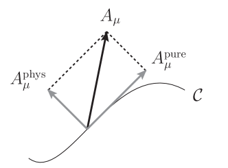
Figure 7: The split of the gauge potential $A_{\mu}$ defined by a contour $\mathcal{C}$. The tangential component is identified with the pure-gauge contribution $A^{\text{pure}}_{\mu}$, and the orthogonal component is identified with the physical contribution $A^{\text{phys}}_{\mu}$.

Changing the contour modifies the split of the gauge potential into pure-gauge and physical contributions. In other words, path dependence is an aspect of Stueckelberg dependence.

From Eq. (250), it is straightforward to see that the matrix $U_{\text{pure}}$ is covariantly conserved

$$D^{\text{pure}}_{\mu}U_{\text{pure}}=0.$$ (260)

This shows, in particular, that the matrix $U_{\text{pure}}$ has no dynamics, and therefore plays the role of a background field. Moreover, for the component along the contour $\mathcal{C}$, one has

$$\frac{\partial s^{\mu}}{\partial\lambda}\,D_{\mu}U_{\text{pure}}=0$$ (261)

which is the familiar parallel transport equation expressing the fact that $U_{\text{pure}}$ does not change along the contour $\mathcal{C}$. The solution of this equation is well known

$$U_{\text{pure}}(x)=\mathcal{W}_{\mathcal{C}}(x,x_{0})\,U_{\text{pure}}(x_{0})$$ (262)

and involves the path-ordered exponential or Wilson line

$$\mathcal{W}_{\mathcal{C}}(b,a)=\mathcal{P}\left[e^{ig\int_{a}^{b}A_{\mu}(s)\,\mathrm{d}s^{\mu}}\right]\equiv\mathds{1}+ig\int_{a}^{b}A_{\mu}(s)\,\mathrm{d}s^{\mu}+(ig)^{2}\int_{a}^{b}\int_{a}^{s_{1}}A_{\mu}(s_{1})A_{\nu}(s_{2})\,\mathrm{d}s^{\mu}_{1}\,\mathrm{d}s^{\nu}_{2}+\cdots.$$ (263)

Using the generic formula for the derivative of the Wilson line

$$\frac{\partial}{\partial z^{\mu}}\mathcal{W}_{\mathcal{C}}(x,y)=ig\,\mathcal{W}_{\mathcal{C}}(x,s)\,A_{\alpha}(s)\,\frac{\partial s^{\alpha}}{\partial z^{\mu}}\,\mathcal{W}_{\mathcal{C}}(s,y)\Big{|}_{s=y}^{s=x}+ig\int_{y}^{x}\mathcal{W}_{\mathcal{C}}(x,s)\,G_{\alpha\beta}(s)\,\mathcal{W}_{\mathcal{C}}(s,y)\,\frac{\partial s^{\alpha}}{\partial z^{\mu}}\,\mathrm{d}s^{\beta},$$ (264)

and the fact that the inverse of the Wilson line is simply given by $\mathcal{W}^{-1}_{\mathcal{C}}(x,y)=\mathcal{W}_{\mathcal{C}}(y,x)$, the pure-gauge and physical fields can be expressed as Lorce:2012ce

$$\begin{split}A^{\text{pure}}_{\mu}(x)&=\frac{i}{g}\,\mathcal{W}_{\mathcal{C}}(x,x_{0})\,\frac{\partial}{\partial x^{\mu}}\mathcal{W}_{\mathcal{C}}(x_{0},x),\\ A^{\text{phys}}_{\mu}(x)&=-\int_{x_{0}}^{x}\mathcal{W}_{\mathcal{C}}(x,s)\,G_{\alpha\beta}(s)\,\mathcal{W}_{\mathcal{C}}(s,x)\,\frac{\partial s^{\alpha}}{\partial x^{\mu}}\,\mathrm{d}s^{\beta}.\end{split}$$ (265)

From the gauge transformation law of the Wilson line

$$\mathcal{W}_{\mathcal{C}}(x,y)\mapsto\tilde{\mathcal{W}}_{\mathcal{C}}(x,y)=U(x)\mathcal{W}_{\mathcal{C}}(x,y)U^{-1}(y),$$ (266)

it is straightforward to check that the pure-gauge and physical fields given in Eq. (265) transform in accordance with Eq. (227). Moreover, different choices of contour $\mathcal{C}$ and reference point $x_{0}$ are easily related to each other. Indeed, denoting the fields obtained with a different contour $\bar{\mathcal{C}}$ and possibly different reference point $\bar{x}_{0}$ with a bar, one can write

$$\bar{U}_{\text{pure}}(x)=U_{\text{pure}}(x)U^{-1}_{S}(x),$$ (267)

where $U_{S}(x)=\bar{U}^{-1}_{\text{pure}}(\bar{x}_{0})\mathcal{W}_{\bar{\mathcal{C}}}(\bar{x}_{0},x)\mathcal{W}_{\mathcal{C}}(x,x_{0})U_{\text{pure}}(x_{0})$ is obviously unitary and gauge invariant. Clearly, Eq. (267) has the generic form of a Stueckelberg transformation (252).

This explicit example illustrates once more that the Chen et al. approach leads to non-local expressions in terms of the full gauge potential $A_{\mu}$. It is because of this non-locality that one can define infinitely many gauge-invariant expressions, as nicely expressed by Bashinsky and Jaffe in Ref. Bashinsky:1998if : “Different ways of gluon-field gauge fixing predetermine different decompositions of the coupled quark-gluon fields into quark and gluon degrees of freedom. Similarly, one can generalize a gauge-variant non-local operator […] to more than one gauge-invariant expressions, raising the problem of deciding which is the true one.”

V.3.2 Generic Lorentz transformations

Let us now discuss the Lorentz transformation properties in non-abelian gauge theories. It is usually implicitly assumed that the quark field has the same Lorentz transformation law in both free and interacting cases

$$\psi(x)\mapsto\psi^{\prime}(x^{\prime})=S[\Lambda]\psi(x),$$ (268)

where $S[\Lambda]$ is the standard matrix representing the Lorentz transformation in Dirac space. Similarly, the ordinary covariant derivative of the quark field is assumed to transform according to

$$D_{\mu}\psi(x)\mapsto D^{\prime}_{\mu}\psi^{\prime}(x^{\prime})=\Lambda_{\mu}^{\phantom{\mu}\nu}S[\Lambda]D_{\nu}\psi(x).$$ (269)

One deduces immediately that the gauge potential transforms as a Lorentz four-vector

$$A_{\mu}(x)\mapsto A^{\prime}_{\mu}(x^{\prime})=\Lambda^{\phantom{\mu}\nu}_{\mu}A_{\nu}(x).$$ (270)

As explained in section IV.4.2, the quark field in a gauge theory transforms as a Dirac spinor only up to a gauge transformations. The generic Lorentz transformation law of the quark and gluon fields are therefore

$$\begin{split}\psi(x)&\mapsto\psi^{\prime}(x^{\prime})=U_{\Lambda}(x)S[\Lambda]\psi(x),\\ A_{\mu}(x)&\mapsto A^{\prime}_{\mu}(x^{\prime})=\Lambda^{\phantom{\mu}\nu}_{\mu}U_{\Lambda}(x)\left[A_{\nu}(x)+\tfrac{i}{g}\,\partial_{\nu}\right]U_{\Lambda}^{-1}(x),\end{split}$$ (271)

where $U_{\Lambda}$ is some $N_{c}\times N_{c}$ unitary matrix in color space associated with the Lorentz transformation $\Lambda$. Clearly, the gauge potential $A_{\mu}$ generally transforms as a connection. Indeed, writing explicitly the internal indices

$$-igA^{a}_{\mu b}\mapsto-igA^{\prime a}_{\mu b}=(\Lambda^{-1})^{\nu}_{\phantom{\nu}\mu}(U^{-1}_{\Lambda})^{d}_{\phantom{d}b}(U_{\Lambda})^{a}_{\phantom{a}c}(-igA^{c}_{\nu d})+(U_{\Lambda})^{a}_{\phantom{a}e}\left[\partial^{\prime}_{\mu}(U^{-1}_{\Lambda})^{e}_{\phantom{e}b}\right]$$ (272)

reveals exactly the same structure as the Lorentz transformation law of the Christoffel symbols in General Relativity

$$\Gamma^{\lambda}_{\mu\nu}\mapsto\Gamma^{\prime\lambda}_{\mu\nu}=\frac{\partial x^{\alpha}}{\partial x^{\prime\mu}}\,\frac{\partial x^{\beta}}{\partial x^{\prime\nu}}\,\frac{\partial x^{\prime\lambda}}{\partial x^{\gamma}}\,\Gamma^{\gamma}_{\alpha\beta}+\frac{\partial x^{\prime\lambda}}{\partial x^{\rho}}\,\frac{\partial^{2}x^{\rho}}{\partial x^{\prime\mu}\partial x^{\prime\nu}},$$ (273)

see e.g. Ref. Soper . The corresponding field-strength tensor generally transforms as

$$G_{\mu\nu}(x)\mapsto G^{\prime}_{\mu\nu}(x^{\prime})=\Lambda^{\phantom{\mu}\alpha}_{\mu}\Lambda^{\phantom{\nu}\beta}_{\nu}U_{\Lambda}(x)G_{\alpha\beta}(x)U^{-1}_{\Lambda},$$ (274)

or more explicitly

$$G^{a}_{\mu\nu b}\mapsto G^{\prime a}_{\mu\nu b}=(\Lambda^{-1})^{\alpha}_{\phantom{\alpha}\mu}(\Lambda^{-1})^{\beta}_{\phantom{\beta}\nu}(U^{-1}_{\Lambda})^{d}_{\phantom{d}b}(U_{\Lambda})^{a}_{\phantom{a}c}G^{c}_{\alpha\beta d},$$ (275)

which has the same structure as the Lorentz transformation law of the Riemann curvature tensor

$$R^{\lambda}_{\phantom{\lambda}\mu\nu\rho}\mapsto R^{\prime\lambda}_{\phantom{\lambda}\mu\nu\rho}=\frac{\partial x^{\alpha}}{\partial x^{\prime\mu}}\,\frac{\partial x^{\beta}}{\partial x^{\prime\nu}}\,\frac{\partial x^{\delta}}{\partial x^{\prime\rho}}\,\frac{\partial x^{\prime\lambda}}{\partial x^{\gamma}}\,R^{\gamma}_{\phantom{\gamma}\alpha\beta\delta}.$$ (276)

The generic Lorentz transformation laws for the non-abelian pure-gauge and physical fields compatible with the Chen et al. approach are given by Lorce:2012rr

$$\begin{split}U_{\text{pure}}(x)&\mapsto U^{\prime}_{\text{pure}}(x^{\prime})=U_{\Lambda}(x)U_{\text{pure}}(x)U^{\text{phys},-1}_{\Lambda}(x),\\ A^{\mu}_{\text{pure}}(x)&\mapsto A^{\prime\mu}_{\text{pure}}(x^{\prime})=\Lambda^{\mu}_{\phantom{\mu}\nu}U_{\Lambda}(x)\left[A^{\nu}_{\text{pure}}(x)+\tfrac{i}{g}\,\partial^{\nu}+C^{\nu}_{\Lambda}(x)\right]U^{-1}_{\Lambda}(x),\\ A^{\mu}_{\text{phys}}(x)&\mapsto A^{\prime\mu}_{\text{phys}}(x^{\prime})=\Lambda^{\mu}_{\phantom{\mu}\nu}U_{\Lambda}(x)\left[A^{\nu}_{\text{phys}}(x)-C^{\nu}_{\Lambda}(x)\right]U^{-1}_{\Lambda}(x),\end{split}$$ (277)

where $C^{\nu}_{\Lambda}(x)=\frac{i}{g}\,U_{\text{pure}}(x)U^{\text{phys},-1}_{\Lambda}(x)\left[\partial^{\nu}U^{\text{phys}}_{\Lambda}(x)\right]U^{-1}_{\text{pure}}(x)$. Similarly to the function $\omega^{\text{phys}}_{\Lambda}(x)$ in Eq. (208), the unitary matrix $U^{\text{phys}}_{\Lambda}(x)$ allows one to preserve the condition defining the physical field under Lorentz transformations. In the abelian case, it simply reads $U^{\text{phys}}_{\Lambda}(x)=e^{ig\omega^{\text{phys}}_{\Lambda}(x)}$.

As in the abelian case, one has the freedom to choose the unitary function $U_{\Lambda}$ thanks to the gauge symmetry. Once again, two options are particularly interesting:

1. To maintain Lorentz covariance explicitly, one may choose to work with $U_{\Lambda}=\mathds{1}$, i.e. with $A^{\mu}$ transforming as a Lorentz four-vector. In this case, the pure-gauge field does not transform as a Lorentz four-vector, since it has to compensate for the non-tensorial nature of the physical field $C^{\nu}_{\Lambda}(x)$. Again, with this choice, Lorentz transformations will generally mix physical and gauge degrees of freedom. For example, suppose that in a given Lorentz frame one has chosen to work in the natural gauge, i.e. with $U_{\text{pure}}=\mathds{1}$ and consequently $A^{\mu}_{\text{pure}}=0$. After a Lorentz transformation, the pure-gauge part becomes $A^{\prime\mu}_{\text{pure}}=\tfrac{i}{g}\,\Lambda^{\mu}_{\phantom{\mu}\nu}U^{\text{phys},-1}_{\Lambda}\partial^{\nu}U^{\text{phys}}_{\Lambda}$. One therefore needs to perform an additional gauge transformation with $U=U^{\text{phys},-1}_{\Lambda}$ in order to recover a vanishing pure-gauge part $\tilde{A}^{\prime\mu}_{\text{pure}}=0$ in the new Lorentz frame.

2. To avoid a mixing between physical and gauge degrees of freedom under Lorentz transformations, one may choose to work with $U_{\Lambda}$ satisfying the condition $(\partial_{\mu}U_{\Lambda})U_{\text{pure}}U^{\text{phys},-1}_{\Lambda}+U_{\Lambda}U_{\text{pure}}(\partial_{\mu}U^{\text{phys},-1}_{\Lambda})=0$. In this case, the gauge potential transforms in the same way as its physical part, while the pure-gauge part undergoes a simple rotation in the internal space on top of a four-vector transformation in the physical space $A^{\prime\mu}_{\text{pure}}=\Lambda^{\mu}_{\phantom{\mu}\nu}U_{\Lambda}A^{\nu}_{\text{pure}}U^{-1}_{\Lambda}$. Consequently, the physical polarizations remain physical under Lorentz transformations, but are generally rotated in the internal space. This internal rotation comes from the fact that different observers may not agree on the color of a quark. Note that when the observers manage to agree on what is “red”, “green” and “blue”, the matrix $U^{\text{phys}}_{\Lambda}$ is expected to reduce to a simple phase factor like in the abelian case.

The generic conclusion in non-abelian gauge theories is therefore the same as in the abelian ones:

$$\begin{split}(A_{\text{pure}})^{\prime\mu}(x^{\prime})&=(A^{\prime\mu})_{\text{pure}}(x^{\prime}),\\ (A_{\text{phys}})^{\prime\mu}(x^{\prime})&=(A^{\prime\mu})_{\text{phys}}(x^{\prime}).\end{split}$$ (278)

The Chen et al. approach is consistent with Lorentz symmetry, and one can write without ambiguity $A_{\text{pure}}^{\prime\mu}(x^{\prime})$ and $A_{\text{phys}}^{\prime\mu}(x^{\prime})$. Note that the matrix $U^{\text{phys}}_{\Lambda}$ can be determined by the Noether’s theorem in the gauge-covariant canonical formalism Lorce:2013gxa . It is such that the Stueckelberg-fixing constraint transforms covariantly under the canonical Lorentz transformations. To the best of our knowledge, this has never been checked explicitly in the non-abelian case so far, and would be an interesting non-trivial result.

V.4 Equivalence with the Dirac formalism based on gauge-invariant variables

We discuss in this section the relation between the Chen et al. approach and a popular approach based on gauge-invariant variables. While they appear rather different at a first sight, they turn out to be related by a unitary transformation, and are in this sense mathematically equivalent.

V.4.1 Generalized Dirac variables

Dirac soon realized that one of the main obstacles in the quantization of a gauge theory is the gauge dependence of the fields. He therefore introduced new variables constructed by adjoining phase factors to the dynamical fields and referred to as Dirac variables Dirac:1955uv . These new variables are non-local functionals of $\psi$ and $A_{\mu}$, but have the advantage of being gauge invariant by construction. They have been rediscovered and generalized several times under different names and in different contexts DeWitt:1962mg ; Mandelstam:1962mi ; Mandelstam:1968hz ; Mandelstam:1968ud ; BialynickiBirula:1963 ; Steinmann:1983ar ; Steinmann:1985id ; Skachkov:1985cz ; Haagensen:1997pi ; Horan:1998im ; Masson:2010vx ; Fournel:2012cr ; Chen:2012vg . We refer to Pervushin:2001kq for a review of the subject. For a comparison between the quantization based on Dirac variables and the more standard Faddeev-Popov approach, see Ref. Lantsman:2006ry .

As already mentioned, the unitary matrix $U_{\text{pure}}$ plays the role of a non-dynamical background field. It can be seen as a non-local functional of the gauge potential which has, in many cases, the form of a Wilson line (262). More importantly, it has the same gauge transformation law as the $\psi$ field. In the spirit of the Dirac approach, one can use $U_{\text{pure}}$ as a phase factor and construct the following new variables Chen:2012vg ; Lorce:2012rr ; Lorce:2013gxa

$$\begin{split}\hat{\psi}(x)&\equiv U^{-1}_{\text{pure}}(x)\psi(x),\\ \hat{A}_{\mu}(x)&\equiv U^{-1}_{\text{pure}}(x)\left[A_{\mu}(x)+\tfrac{i}{g}\,\partial_{\mu}\right]U_{\text{pure}}(x).\end{split}$$ (279)

Clearly, following Eq. (251), these variables are by construction gauge invariant and represent the generic form of any kind of Dirac variable. In this sense, these new variables are referred to as generalized Dirac variables. Sometimes, the gauge-invariant fields $\hat{\psi}$ and $\hat{A}_{\mu}$ are interpreted as dressed quark and gluon fields. Accordingly, the matrix $U_{\text{pure}}$ is called the dressing field. From a geometrical point of view, $U_{\text{pure}}$ simply specifies a reference configuration in the internal space Lorce:2012rr . The gauge-invariant fields $\hat{\psi}$ and $\hat{A}_{\mu}$ then represent “physical” deviations from this reference configuration. This is supported by the following observations

$$\begin{split}\hat{A}^{\text{pure}}_{\mu}(x)&\equiv U^{-1}_{\text{pure}}(x)\left[A^{\text{pure}}_{\mu}(x)+\tfrac{i}{g}\,\partial_{\mu}\right]U_{\text{pure}}(x)\\ &=0,\\ \hat{A}^{\text{phys}}_{\mu}(x)&\equiv U^{-1}_{\text{pure}}(x)A^{\text{phys}}_{\mu}(x)U_{\text{pure}}(x)\\ &=\hat{A}_{\mu}(x),\\ \hat{G}_{\mu\nu}(x)&\equiv U^{-1}_{\text{pure}}(x)G_{\mu\nu}(x)U_{\text{pure}}(x)\\ &=\partial_{\mu}\hat{A}_{\nu}(x)-\partial_{\nu}\hat{A}_{\mu}(x)-ig[\hat{A}_{\mu}(x),\hat{A}_{\nu}(x)].\end{split}$$ (280)

We stress that, despite appearances, Eq. (279) does not represent a gauge transformation, but is a definition of new variables in any gauge. This should not be confused with the fact that after a gauge transformation with $U(x)=U^{-1}_{\text{pure}}(x)$, one has

$$\begin{split}\tilde{\psi}(x)&=\hat{\psi}(x),\\ \tilde{A}_{\mu}(x)&=\hat{A}_{\mu}(x).\end{split}$$ (281)

The generalized Dirac variables $\hat{\psi}$ and $\hat{A}_{\mu}$, being defined in any gauge, can therefore be interpreted as the natural gauge-invariant extensions of the original gauge non-invariant fields $\psi$ and $A_{\mu}$.

V.4.2 The Dirac gauge-invariant approach

In the Dirac gauge-invariant approach, one first rewrites the standard QCD Lagrangian

$$\mathcal{L}_{\text{QCD}}(x)=f[\psi(x),\partial_{\mu}\psi(x),A_{\nu}(x),\partial_{\mu}A_{\nu}(x)]$$ (282)

in terms of the new gauge-invariant variables $\hat{\psi}$ and $\hat{A}_{\mu}$

$$\mathcal{L}_{\text{QCD}}(x)=f[\hat{\psi}(x),\partial_{\mu}\hat{\psi}(x),\hat{A}_{\nu}(x),\partial_{\mu}\hat{A}_{\nu}(x)].$$ (283)

This is of course always possible thanks to the gauge symmetry and the fact that the generalized Dirac variables are the gauge-invariant extensions of the original quark and gluon fields.

Since the Lagrangian now involves only gauge-invariant variables, one can simply apply the standard canonical formalism to derive the QCD equations of motion

$$(i\,/\!\!\!\!\hat{D}-m)\hat{\psi} =0,$$ (284)

$$2(\hat{\mathcal{D}}_{\alpha}\hat{G}^{\alpha\mu})^{a}_{\phantom{a}b} =-g\hat{\overline{\psi}}_{b}\gamma^{\mu}\hat{\psi}^{a},$$ (285)

where the gauge-invariant derivatives are given by $\hat{D}_{\mu}=\partial_{\mu}-ig\hat{A}_{\mu}$ and $\hat{\mathcal{D}}_{\mu}=\partial_{\mu}-ig[\hat{A}_{\mu},\quad]$. From Noether’s theorem, one obtains the following gauge-invariant expressions for the generators of Poincaré transformations

$$\hat{T}^{\mu\nu} =\tfrac{1}{2}\,\hat{\overline{\psi}}\gamma^{\mu}i\overset{\leftrightarrow}{\partial}\!\!\!\!\phantom{\partial}^{\nu}\hat{\psi}-2\,\mathrm{Tr}[\hat{G}^{\mu\alpha}\partial^{\nu}\hat{A}_{\alpha}]-g^{\mu\nu}\mathcal{L}_{\text{QCD}},$$ (286)

$$\hat{M}^{\mu\nu\rho} =\tfrac{1}{2}\,\epsilon^{\mu\nu\rho\sigma}\,\hat{\overline{\psi}}\gamma_{\sigma}\gamma_{5}\hat{\psi}+\tfrac{1}{2}\,\hat{\overline{\psi}}\gamma^{\mu}x^{[\nu}i\overset{\leftrightarrow}{\partial}\!\!\!\!\phantom{\partial}^{\rho]}\hat{\psi}-2\,\mathrm{Tr}[\hat{G}^{\mu[\nu}\hat{A}^{\rho]}]-2\,\mathrm{Tr}[\hat{G}^{\mu\alpha}x^{[\nu}\partial^{\rho]}\hat{A}_{\alpha}]-x^{[\nu}g^{\rho]\mu}\mathcal{L}_{\text{QCD}}.$$ (287)

They are naturally split into quark and gluon contributions as follows

$$\hat{T}^{\mu\nu}_{q,\text{M}} =\tfrac{1}{2}\,\hat{\overline{\psi}}\gamma^{\mu}i\overset{\leftrightarrow}{\partial}\!\!\!\!\phantom{\partial}^{\nu}\hat{\psi}, \hat{T}^{\mu\nu}_{G,\text{M}} =-2\,\mathrm{Tr}[\hat{G}^{\mu\alpha}\partial^{\nu}\hat{A}_{\alpha}],$$ (288)

$$\hat{T}^{\mu\nu}_{q,\text{E}} =-g^{\mu\nu}\hat{\mathcal{L}}_{\text{D}}, \hat{T}^{\mu\nu}_{G,\text{E}} =-g^{\mu\nu}(\hat{\mathcal{L}}_{\text{YM}}+\hat{\mathcal{L}}_{\text{int}}),$$

$$\hat{M}^{\mu\nu\rho}_{q,\text{spin}} =\tfrac{1}{2}\,\epsilon^{\mu\nu\rho\sigma}\,\hat{\overline{\psi}}\gamma_{\sigma}\gamma_{5}\hat{\psi}, \hat{M}^{\mu\nu\rho}_{G,\text{spin}} =-2\,\mathrm{Tr}[\hat{G}^{\mu[\nu}\hat{A}^{\rho]}],$$

$$\hat{M}^{\mu\nu\rho}_{q,\text{OAM}} =\tfrac{1}{2}\,\hat{\overline{\psi}}\gamma^{\mu}x^{[\nu}i\overset{\leftrightarrow}{\partial}\!\!\!\!\phantom{\partial}^{\rho]}\hat{\psi}, \hat{M}^{\mu\nu\rho}_{G,\text{OAM}} =-2\,\mathrm{Tr}[\hat{G}^{\mu\alpha}x^{[\nu}\partial^{\rho]}\hat{A}_{\alpha}],$$

$$\hat{M}^{\mu\nu\rho}_{q,\text{boost}} =-x^{[\nu}g^{\rho]\mu}\hat{\mathcal{L}}_{\text{D}}, \hat{M}^{\mu\nu\rho}_{G,\text{boost}} =-x^{[\nu}g^{\rho]\mu}(\hat{\mathcal{L}}_{\text{YM}}+\hat{\mathcal{L}}_{\text{int}}),$$

where

$$\begin{split}\hat{\mathcal{L}}_{\text{D}}&=\hat{\overline{\psi}}(\tfrac{i}{2}\,/\!\!\!\!\overset{\leftrightarrow}{\partial}\!\!\!\!\phantom{\partial}-m)\hat{\psi},\\ \hat{\mathcal{L}}_{\text{YM}}&=-\tfrac{1}{2}\,\mathrm{Tr}[\hat{G}^{\mu\nu}\hat{G}_{\mu\nu}],\\ \hat{\mathcal{L}}_{\text{int}}&=g\hat{\overline{\psi}}\,/\!\!\!\!\hat{A}\hat{\psi},\end{split}$$ (289)

which have exactly the structure of the canonical expressions, with $\psi$ and $A^{\mu}$ replaced by the gauge-invariant fields $\hat{\psi}$ and $\hat{A}_{\mu}$, respectively. In particular, the corresponding gauge-invariant linear and angular momentum operators are, respectively, generators of translations and rotations for the gauge-invariant quark and gluon fields, i.e. satisfy the following equal-time commutation relations

$$\,[\hat{P}^{i}_{q},\hat{\psi}] =-\tfrac{1}{i}\nabla^{i}\hat{\psi}, [\hat{P}^{i}_{G},\hat{A}^{j}] =-\tfrac{1}{i}\nabla^{i}\hat{A}^{j},$$ (290)

$$[\hat{S}^{i}_{q},\hat{\psi}] =-\tfrac{1}{2}\Sigma^{i}\hat{\psi}, [\hat{S}^{i}_{G},\hat{A}^{j}] =-(-i\epsilon^{ijk})\hat{A}^{k},$$

$$[\hat{L}^{i}_{q},\hat{\psi}] =-(\bm{x}\times\tfrac{1}{i}\bm{\nabla})^{i}\hat{\psi}, [\hat{L}^{i}_{G},\hat{A}^{j}] =-(\bm{x}\times\tfrac{1}{i}\bm{\nabla})^{i}\hat{A}^{j},$$

where

$$\hat{P}^{i}_{q} =\int\mathrm{d}^{3}x\,\hat{T}^{0i}_{q,\text{M}}, \hat{P}^{i}_{G} =\int\mathrm{d}^{3}x\,\hat{T}^{0i}_{G,\text{M}},$$ (291)

$$\hat{S}^{i}_{q} =\tfrac{1}{2}\,\epsilon^{ijk}\int\mathrm{d}^{3}x\,\hat{M}^{0jk}_{q,\text{spin}}, \hat{S}^{i}_{G} =\tfrac{1}{2}\,\epsilon^{ijk}\int\mathrm{d}^{3}x\,\hat{M}^{0jk}_{G,\text{spin}},$$

$$\hat{L}^{i}_{q} =\tfrac{1}{2}\,\epsilon^{ijk}\int\mathrm{d}^{3}x\,\hat{M}^{0jk}_{q,\text{OAM}}, \hat{L}^{i}_{G} =\tfrac{1}{2}\,\epsilon^{ijk}\int\mathrm{d}^{3}x\,\hat{M}^{0jk}_{G,\text{OAM}}.$$

One sees that choosing gauge-invariant fields $\hat{\psi}$ and $\hat{A}_{\mu}$ as the canonical variables leads naturally to gauge-invariant canonical linear and angular momentum operators. The rule of thumb is particularly simple: it suffices to replace in every standard canonical expression the gauge non-invariant fields $\psi$ and $A_{\mu}$ by the corresponding generalized Dirac variable $\hat{\psi}$ and $\hat{A}_{\mu}$, in order to obtain the gauge-invariant expressions. Interestingly, Chen Chen:2012vg rediscovered Dirac variables precisely while trying to derive gauge-invariant equations of the type (290) and (291).

V.4.3 Equivalence with the Chen et al. approach

The decomposition (288) mimics perfectly the Jaffe-Manohar decomposition (231), except that the fields involved are now gauge invariant. As observed by Chen Chen:2012vg and further explored by Lorcé Lorce:2012rr ; Lorce:2013gxa , the decomposition (288) is just the gauge-invariant canonical decomposition (233) written in terms of the gauge-invariant variables $\hat{\psi}$ and $\hat{A}_{\mu}$

$$\hat{T}^{\mu\nu} =T^{\mu\nu}_{\text{gic}}\Big{|}_{\begin{subarray}{l}\quad\,\,\,\psi\mapsto U^{-1}_{\text{pure}}\hat{\psi}\\ A^{\text{pure}}_{\mu}\mapsto\tfrac{i}{g}\,U_{\text{pure}}\partial_{\mu}U^{-1}_{\text{pure}}\\ A^{\text{phys}}_{\mu}\mapsto U_{\text{pure}}\hat{A}_{\mu}U^{-1}_{\text{pure}}\end{subarray}}, \qquad\hat{M}^{\mu\nu\rho} =M^{\mu\nu\rho}_{\text{gic}}\Big{|}_{\begin{subarray}{l}\quad\,\,\,\psi\mapsto U^{-1}_{\text{pure}}\hat{\psi}\\ A^{\text{pure}}_{\mu}\mapsto\tfrac{i}{g}\,U_{\text{pure}}\partial_{\mu}U^{-1}_{\text{pure}}\\ A^{\text{phys}}_{\mu}\mapsto U_{\text{pure}}\hat{A}_{\mu}U^{-1}_{\text{pure}}\end{subarray}}.$$ (292)

Indeed, one can easily see that

$$\begin{split}\partial_{\mu}\hat{\psi}&=U^{-1}_{\text{pure}}D^{\text{pure}}_{\mu}\psi,\\ \partial_{\mu}\hat{A}_{\nu}&=U^{-1}_{\text{pure}}[\mathcal{D}^{\text{pure}}_{\mu}A^{\text{phys}}_{\nu}]U_{\text{pure}}.\end{split}$$ (293)

The commutation relations (290) can therefore be rewritten as

$$\,[P^{q,i}_{\text{gic}},\psi] =-iD^{i}_{\text{pure}}\psi, [P^{G,i}_{\text{gic}},A^{j}_{\text{phys}}] =-i\mathcal{D}^{i}_{\text{pure}}A^{j}_{\text{phys}},$$ (294)

$$[S^{q,i}_{\text{gic}},\psi] =-\tfrac{1}{2}\Sigma^{i}\psi, [S^{G,i}_{\text{gic}},A^{j}_{\text{phys}}] =-(-i\epsilon^{ijk})A^{k}_{\text{phys}},$$

$$[L^{q,i}_{\text{gic}},\psi] =-(\bm{x}\times i\bm{D}_{\text{pure}})^{i}\psi, [L^{G,i}_{\text{gic}},A^{j}_{\text{phys}}] =-(\bm{x}\times i\bm{\mathcal{D}}_{\text{pure}})^{i}A^{j}_{\text{phys}},$$

and are consistent with the gauge-covariant canonical formalism based on the Chen et al. approach Lorce:2013gxa .

Clearly, the Chen et al. and Dirac gauge-invariant approaches are mathematically equivalent, since they are simply related by a unitary transformation of the variables. This also means that the issue of uniqueness raised by the Stueckelberg symmetry affects the Dirac approach as well. Indeed, even if the generalized Dirac variables are gauge invariant, they change under the Stueckelberg transformations

$$\begin{split}\hat{\psi}(x)&\mapsto\hat{\bar{\psi}}(x)=U_{S}(x)\hat{\psi}(x),\\ \hat{A}_{\mu}(x)&\mapsto\hat{\bar{A}}_{\mu}(x)=U_{S}(x)\left[\hat{A}_{\mu}(x)+\tfrac{i}{g}\,\partial_{\mu}\right]U^{-1}_{S}(x),\\ \hat{A}^{\text{pure}}_{\mu}(x)&\mapsto\hat{\bar{A}}^{\text{pure}}_{\mu}(x)=U_{S}(x)\hat{A}^{\text{pure}}_{\mu}(x)U^{-1}_{S}(x),\\ \hat{A}^{\text{phys}}_{\mu}(x)&\mapsto\hat{\bar{A}}^{\text{phys}}_{\mu}(x)=U_{S}(x)\left[\hat{A}^{\text{phys}}_{\mu}(x)+\tfrac{i}{g}\,\partial_{\mu}\right]U^{-1}_{S}(x).\end{split}$$ (295)

There is exactly the same freedom in defining precisely the generalized Dirac variables $\hat{\psi}$ and $\hat{A}_{\mu}$ as in defining a precise split $A_{\mu}=A^{\text{pure}}_{\mu}+A^{\text{phys}}_{\mu}$. The existence of an entire class of composite gauge-invariant fields was already pointed out by Dirac and Steinmann Dirac:1955uv ; Steinmann:1983ar ; Steinmann:1985id . Note in particular that the Dirac gauge-invariant formulation of QED Dirac:1955uv is equivalent to the original three-dimensional Chen et al. approach based on the Coulomb constraint $\bm{\nabla}\cdot\bm{A}_{\text{phys}}=0$ Chen:2008ag , since both make use of the phase factor

$$U_{\text{pure}}(x)=e^{ie\frac{\bm{\nabla}\cdot\bm{A}(x)}{\bm{\nabla}^{2}}},$$ (296)

which is the dressing factor associated with the Coulomb GIE. By construction, they give the same results as the standard approach to QED restricted to the Coulomb gauge. For the contour-based gauge-invariant extensions defined by Eq. (258), the explicit non-local expressions for the generalized Dirac variables are

$$\begin{split}\hat{\psi}(x)&=\mathcal{W}_{\mathcal{C}}(x_{0},x)\psi(x),\\ \hat{A}_{\mu}(x)&=-\int_{x_{0}}^{x}\hat{G}_{\alpha\beta}(s)\,\frac{\partial s^{\alpha}}{\partial x^{\mu}}\,\mathrm{d}s^{\beta}\\ &=-\int_{x_{0}}^{x}\mathcal{W}_{\mathcal{C}}(x_{0},s)G_{\alpha\beta}(s)\mathcal{W}_{\mathcal{C}}(s,x_{0})\,\frac{\partial s^{\alpha}}{\partial x^{\mu}}\,\mathrm{d}s^{\beta},\end{split}$$ (297)

with $\mathcal{W}_{\mathcal{C}}(b,a)$ given by Eq. (263) and where we have set $U_{\text{pure}}(x_{0})=\mathds{1}$ for simplicity thanks to the invariance under global (i.e. $x$-independent) rotations in internal space.

VI Angular momentum sum rules and relations

It is of great interest to try to derive sum rules, which follow rigorously from QCD, relating experimentally measurable quantities, because checking such sum rules then provides a searching test of the theory upon which the derivation is based. Sometimes it is not possible to measure every term in a sum rule. Strictly speaking such a relation should then not be called a sum rule, but it may still be of value in checking the validity of model calculations of some of the terms in the relation. Angular momentum sum rules, relating the angular momentum of a hadron, usually a nucleon, to the angular momentum of its constituents, are of particular interest at present and much effort, both theoretical and experimental, is being devoted to studying them.

VI.1 General overview

There are now five angular momentum relations or sum rules for the nucleon in the literature: the Jaffe-Manohar (JM) relation for a longitudinally polarized nucleon Jaffe:1989jz , and the Bakker-Leader-Trueman (BLT) result for the case of transverse polarization Bakker:2004ib ; the Ji relation for longitudinal polarization Ji:1997pf ; Ji:1996ek ; Ji:1996nm , and the Leader result for transverse polarization Leader:2011cr , both the latter involving generalized parton distributions; and a new sum rule due to Ji, Xiong and Yuan dealing with the transverse component of the Pauli-Lubanski vector Ji:2012vj . In addition to these, Harindranath and Kundu Harindranath:1998ve have shown how the JM sum rule can be derived from a study of the light-front rotation operator about the $OZ$ axis, and Harindranath, Kundu and Ratabole Harindranath:2001rc ; Harindranath:1999ve have discussed an interesting sum rule based on the transverse light-front spin operators. Since these are interaction dependent, the analysis involves a perturbative QCD treatment and we shall not discuss this paper here.

We shall discuss these various relations and examine their precise interpretation in the light of the “angular momentum controversy”. In particular, we shall show that the claim of Ji, Xiong and Yuan (JXY) that their Pauli-Lubanski relation is frame or energy independent is incorrect, and that they have discarded an energy-dependent term in their expression. A different point of view is taken in Ref. Harindranath:2013goa and this will be discussed later.

Generally speaking, the above sum rules fall into two classes. In the JM and BLT relations, one obtains an expression for the nucleon matrix elements of the angular momentum operators and then substitutes a Fock expansion for the nucleon state in terms of quarks and gluons. In the Ji and Leader relations, one expresses the nucleon matrix elements of the angular momentum operators in terms of nucleon matrix elements of the energy-momentum density, and then relates these matrix elements to quark and gluon generalized parton distributions (GPDs). The JXY case is somewhat different, as will become clear later.

VI.2 Expectation values of operators

In order to derive sum rules, we will need to evaluate the expectation values of the momentum and angular momentum operators. Using the conventional relativistic state normalization

$$\langle P^{\prime}|P\rangle=2P^{0}\,(2\pi)^{3}\,\delta^{(3)}(\bm{P}^{\prime}-\bm{P}),$$ (298)

the expectation value of any operator $\hat{O}$ is given in terms of its forward matrix elements as

$$\langle\langle P|\hat{O}|P\rangle\rangle=\frac{\langle P|\hat{O}|P\rangle}{2P^{0}\,(2\pi)^{3}\,\delta^{(3)}(\bm{0})}.$$ (299)

For the total momentum and angular momentum of the system, in this case the nucleon, the operators are time-independent, so that their expectation values are simply numerical functions of the momentum and spin of the nucleon. The situation appears, at first sight, to be completely different when we separate, say, the momentum $P^{\mu}$ of the nucleon into contributions from quarks and gluons. Thus the oft written equation

$$P^{\mu}=\sum_{q}P^{\mu}_{q}+P^{\mu}_{G}$$ (300)

as it stands, is somewhat misleading, and should be written

$$P^{\mu}=\sum_{q}P^{\mu}_{q}(t)+P^{\mu}_{G}(t)$$ (301)

to reflect the fact that the quark and gluon momentum operators are not separately conserved, since the quarks and gluons exchange momentum as a result of their interaction.

Nonetheless, as we shall now show, the matrix elements between states of the same energy, and thus the expectation values, of $P^{\mu}_{q}(t)$ and $P^{\mu}_{G}(t)$ are time-independent, so that it does make sense to talk about e.g. the quark contribution to the nucleon momentum. To see this for the momentum $P_{q}^{\mu}(t)$, which is expressed as a spatial integral of the quark part of the momentum density $T^{0\mu}_{q}(x)$, let

$$|\psi\rangle=\int\mathrm{d}^{3}p^{\prime}\,\psi(\bm{p}^{\prime})\,|\bm{p}^{\prime}\rangle\quad\textrm{and}\quad|\phi\rangle=\int\mathrm{d}^{3}p\,\phi(\bm{p})\,|\bm{p}\rangle$$ (302)

be arbitrary states of a free particle of mass $m$, with the same energy, so that

$$(p^{0})^{2}=\bm{p}^{2}+m^{2}=(p^{\prime 0})^{2}=\bm{p}^{\prime 2}+m^{2}.$$ (303)

Then

$$\langle\psi|P_{q}^{\mu}(t)|\phi\rangle = \int\mathrm{d}^{3}p^{\prime}\,\mathrm{d}^{3}p\,\mathrm{d}^{3}x\,\psi^{*}(\bm{p}^{\prime})\,\phi(\bm{p})\,\langle\bm{p}^{\prime}|T_{q}^{0\mu}(x)|\bm{p}\rangle$$ (304)

$$= \int\mathrm{d}^{3}p^{\prime}\,\mathrm{d}^{3}p\,\mathrm{d}^{3}x\,\psi^{*}(\bm{p}^{\prime})\,\phi(\bm{p})\,e^{-i(\bm{p}^{\prime}-\bm{p})\cdot\bm{x}}\,e^{i(p^{\prime 0}-p^{0})t}\,\langle\bm{p}^{\prime}|T_{q}^{0\mu}(0)|\bm{p}\rangle$$

$$= (2\pi)^{3}\int\mathrm{d}^{3}p^{\prime}\,\mathrm{d}^{3}p\,\psi^{*}(\bm{p}^{\prime})\,\phi(\bm{p})\,\delta^{(3)}(\bm{p}^{\prime}-\bm{p})\,e^{i(p^{\prime 0}-p^{0})t}\,\langle\bm{p}^{\prime}|T_{q}^{0\mu}(0)|\bm{p}\rangle$$

$$= (2\pi)^{3}\int\mathrm{d}^{3}p\,\psi^{*}(\bm{p})\,\phi(\bm{p})\,\langle\bm{p}|T_{q}^{0\mu}(0)|\bm{p}\rangle$$

which is independent of time because $p^{\prime 0}=p^{0}$.

A similar, though more complicated, argument shows that the matrix elements of the angular momentum operator $\bm{J}_{q,G}(t)$, between states of equal energy, are also time-independent.

VI.3 Relation between the matrix elements of angular momentum and energy-momentum density

One of the key steps in deriving angular momentum sum rules involves relating the matrix elements of the angular momentum operator to those of the energy-momentum density, and this turns out to be a very subtle issue, with incorrect results appearing in several papers in the literature. Whether one is considering the orbital part of the canonical version $M^{\nu\rho}$ or the Belinfante version $M^{\nu\rho}_{\text{Bel}}$ of the angular momentum operator, one is faced with the problem of evaluating the expectation value of a compound operator of the form $x^{\nu}T^{\mu\rho}-x^{\rho}T^{\mu\nu}$. For example consider Eq. (II.6.2)

$$\langle P,\mathscr{S}|M^{\nu\rho}_{\text{Bel}}|P,\mathscr{S}\rangle = \int\mathrm{d}^{3}x\,\langle P,\mathscr{S}|M^{0\nu\rho}_{\text{Bel}}(x)|P,\mathscr{S}\rangle$$ (305)

$$= \int\mathrm{d}^{3}x\,\langle P,\mathscr{S}|x^{\nu}T^{0\rho}_{\text{Bel}}(x)-x^{\rho}T^{0\nu}_{\text{Bel}}(x)|P,\mathscr{S}\rangle.$$

Using the fact that $T^{\mu\nu}_{\text{Bel}}(x)$ is a local operator, this becomes

$$\langle P,\mathscr{S}|M^{\nu\rho}_{\text{Bel}}|P,\mathscr{S}\rangle = \int\mathrm{d}^{3}x\,x^{\nu}\,\langle P,\mathscr{S}|e^{iP\cdot x}\,T^{0\rho}_{\text{Bel}}(0)\,e^{-iP\cdot x}|P,\mathscr{S}\rangle-(\nu\leftrightarrow\rho)$$ (306)

$$= \int\mathrm{d}^{3}x\,x^{\nu}\,\langle P,\mathscr{S}|T^{0\rho}_{\text{Bel}}(0)|P,\mathscr{S}\rangle-(\nu\leftrightarrow\rho).$$

Now the matrix element in Eq. (306) is independent of $x$, so that the integral $\int\mathrm{d}^{3}x\,x^{\nu}$ is totally ambiguous, being either infinite or, by symmetry, zero.

This kind of problem is typical of what happens, even in non-relativistic Quantum Mechanics, when one uses plane-wave states, and the solution is well known. One must use normalized wave packets which are superpositions of physical plane-wave states. A possible example is a packet with momentum localized around the value $\bar{\bm{P}}$

$$|\phi_{\bar{\bm{P}}}\rangle=\int\mathrm{d}^{3}P\,\phi_{\bar{\bm{P}}}(\bm{P})\,|\bm{P}\rangle=\mathcal{N}\int\mathrm{d}^{3}P\,e^{-\lambda^{2}(\bm{P}-\bar{\bm{P}})^{2}}\,|\bm{P}\rangle,$$ (307)

where $\mathcal{N}$ is a normalization constant, and where, at the end, one takes the limit $\lambda\rightarrow\infty$.

The generalization of this to particles with spin is not discussed in non-relativistic Quantum Mechanics and one has to be aware of certain subtleties arising in the relativistic case. For example, for a spin-$1/2$ particle it is often convenient, as above, to specify its state in the form $|P,\mathscr{S}\rangle$ where $P^{\mu}=(\sqrt{\bm{P}^{2}+M^{2}},\bm{P})$ and $\mathscr{S}^{\mu}$ is the covariant spin vector. It is then incorrect to regard the following as an acceptable physical wave packet centered around the momentum $\bar{P}$:

$$|\phi_{\bar{P},\mathscr{S}}\rangle=\mathcal{N}\,\int\mathrm{d}^{3}P\,\phi_{\bar{P}}(\bm{P})\,|P,\mathscr{S}\rangle$$ (308)

for the simple reason that $\mathscr{S}^{\mu}$ is a function of $\bm{P}$ satisfying

$$P\cdot\mathscr{S}=0,$$ (309)

and so cannot be kept fixed if one integrates freely over the momenta in the superposition. The desire, in certain papers, to use the above form with fixed $\mathscr{S}^{\mu}$, stems from the fact that it simplifies calculations, which, however, are then incorrect. Failure to recognize this and to respect Eq. (309) has led to errors in the literature Jaffe:1989jz ; Wakamatsu:2010cb .

The correct way to build a physical wave packet for a spin-$1/2$ particle was given in Bakker, Leader and Trueman (BLT) Bakker:2004ib and utilizes the relation between $\mathscr{S}^{\mu}$, normalized to $\mathscr{S}^{2}=-M^{2}$, and the rest-frame spin vector $\bm{s}$, namely

$$\mathscr{S}^{\mu}=\mathfrak{S}^{\mu}(P,\bm{s})\equiv\left(\bm{P}\cdot\bm{s},M\bm{s}+\frac{\bm{P}\cdot\bm{s}}{P^{0}+M}\,\bm{P}\right)$$ (310)

to build a wave packet as a superposition of momentum eigenstates with fixed rest-frame spin vector i.e.

$$|\phi_{\bar{P},\bm{s}}\rangle=\mathcal{N}\,\int\mathrm{d}^{3}P\,\phi_{\bar{P}}(\bm{P})\,|P,\bm{s}\rangle.$$ (311)

However, the use of wave packets to regulate the integral in Eq. (306), while rigorous, is extremely cumbersome, so we shall now turn to a different approach suggested by Jaffe and Manohar Jaffe:1989jz but, unfortunately, incorrectly used by them. They begin their analysis by considering the non-forward quantity

$$\mathcal{M}^{\mu\nu\rho}(P,k,P^{\prime},\mathscr{S})\equiv\int\mathrm{d}^{4}x\,e^{ik\cdot x}\,\langle P^{\prime},\mathscr{S}|M^{\mu\nu\rho}(x)|P,\mathscr{S}\rangle.$$ (312)

One may wonder why a four-dimensional Fourier transform is introduced in dealing with a three-dimensional integral. The reason is that $\mathcal{M}^{\mu\nu\rho}(P,k,P^{\prime},\mathscr{S})$ seems to transform as a Lorentz tensor, but that is an illusion, because the non-forward matrix element of a tensor operator is not a tensor Bakker:2004ib . This misunderstanding is partly responsible for the error in Ref. Jaffe:1989jz mentioned above. Note that strictly speaking, as discussed above, the covariant four-vector $\mathscr{S}$ in the final state cannot be the same as in the initial state, since for a physical nucleon one must have $P\cdot\mathscr{S}=P^{\prime}\cdot\mathscr{S}^{\prime}=0$ leading generally to $\mathscr{S}\neq\mathscr{S}^{\prime}$. The correct way to handle Eq. (312) is to specify the same rest-frame vector $\bm{s}$ in both initial and final states.

Since nothing is gained by using a four-dimensional Fourier transform, we modify the JM approach by rewriting Eq. (306) in the form

$$\langle P,\mathscr{S}|M^{\nu\rho}_{\text{Bel}}|P,\mathscr{S}\rangle = \int\mathrm{d}^{3}x\,x^{\nu}\,\langle P,\mathscr{S}|e^{iP^{0}t}\,T^{0\rho}_{\text{Bel}}(0,\bm{x})\,e^{-iP^{0}t}|P,\mathscr{S}\rangle-(\nu\leftrightarrow\rho)$$ (313)

$$= \int\mathrm{d}^{3}x\,x^{\nu}\,\langle P,\mathscr{S}|T^{0\rho}_{\text{Bel}}(0,\bm{x})|P,\mathscr{S}\rangle-(\nu\leftrightarrow\rho),$$

and then evaluating the RHS via

$$\langle\,P,\mathscr{S}|M^{\nu\rho}_{\text{Bel}}|P,\mathscr{S}\rangle = \lim_{\bm{\Delta}\rightarrow\bm{0}}\int\mathrm{d}^{3}x\,\langle P+\tfrac{\Delta}{2},\mathscr{S}_{f}|x^{\nu}T^{0\rho}_{\text{Bel}}(0,\bm{x})-x^{\rho}T^{0\nu}_{\text{Bel}}(0,\bm{x})|P-\tfrac{\Delta}{2},\mathscr{S}_{i}\rangle$$ (314)

$$= \lim_{\bm{\Delta}\rightarrow\bm{0}}\int\mathrm{d}^{3}x\,e^{-i\bm{\Delta}\cdot\bm{x}}\langle P+\tfrac{\Delta}{2},\mathscr{S}_{f}|x^{\nu}T^{0\rho}_{\text{Bel}}(0)-x^{\rho}T^{0\nu}_{\text{Bel}}(0)|P-\tfrac{\Delta}{2},\mathscr{S}_{i}\rangle,$$

where, see Eq. (310),

$$\mathscr{S}_{i}^{\mu}=\mathfrak{S}^{\mu}(P-\tfrac{\Delta}{2},\bm{s}),\qquad\mathscr{S}_{f}^{\mu}=\mathfrak{S}^{\mu}(P+\tfrac{\Delta}{2},\bm{s}).$$ (315)

It is crucial to understand that the four components of $\Delta^{\mu}$ are not independent. This follows from the mass-shell conditions $(P\pm\tfrac{\Delta}{2})^{2}=M^{2}$ which imply

$$P\cdot\Delta=0\qquad\text{or}\qquad\Delta^{0}=\frac{\bm{P}\cdot\bm{\Delta}}{P^{0}},$$ (316)

so that the limit $\bm{\Delta}\rightarrow\bm{0}$ implies that $\Delta^{\mu}\rightarrow 0$, and also that $\mathscr{S}_{i}\rightarrow\mathscr{S}$ and $\mathscr{S}_{f}\rightarrow\mathscr{S}$. Note that the physical requirements $(P-\tfrac{\Delta}{2})\cdot\mathscr{S}_{i}=0$ and $(P+\tfrac{\Delta}{2})\cdot\mathscr{S}_{f}=0$ are satisfied automatically and do not put any further constraints on the components of $\Delta^{\mu}$. In summary, the essential point is that the three spatial components of $\Delta^{\mu}$ should be taken as independent variables and so, when differentiating with respect to say $\Delta^{j}$ ($j=1,2,3$), it must not be forgotten, as has happened in some analyses, that $\Delta^{0}$ is a function of $\Delta^{j}$.

Consider now the expression for the actual angular momentum operators

$$\langle P,\mathscr{S}|M^{jk}_{\text{Bel}}|P,\mathscr{S}\rangle = \lim_{\bm{\Delta}\rightarrow\bm{0}}\int\mathrm{d}^{3}x\,e^{-i\bm{\Delta}\cdot\bm{x}}\langle P+\tfrac{\Delta}{2},\mathscr{S}_{f}|x^{j}T^{0k}_{\text{Bel}}(0)-x^{k}T^{0j}_{\text{Bel}}(0)|P-\tfrac{\Delta}{2},\mathscr{S}_{i}\rangle$$ (317)

$$= \lim_{\bm{\Delta}\rightarrow\bm{0}}\int\mathrm{d}^{3}x\left[i\,\frac{\partial}{\partial\Delta^{j}}\,e^{-i\bm{\Delta}\cdot\bm{x}}\right]\langle P+\tfrac{\Delta}{2},\mathscr{S}_{f}|T^{0k}_{Bel}(0)|P-\tfrac{\Delta}{2},\mathscr{S}_{i}\rangle-(j\leftrightarrow k).$$

We now use the Leibniz product rule to write the derivative of the exponential as the derivative of the entire expression minus the exponential times the derivative of the matrix element. The former, as shown by the wave-packet analysis of BLT, measures the angular momentum of the wave packet about the origin of coordinates, and the latter measures the internal angular momentum of the nucleon. Only the latter is of interest and yields

$$\langle P,\mathscr{S}|M^{jk}_{\text{Bel}}|P,\mathscr{S}\rangle=\lim_{\bm{\Delta}\rightarrow\bm{0}}\int\mathrm{d}^{3}x\,e^{-i\bm{\Delta}\cdot\bm{x}}\,(-i)\,\frac{\partial}{\partial\Delta^{j}}\langle P+\tfrac{\Delta}{2},\mathscr{S}_{f}|T^{0k}_{\text{Bel}}(0)|P-\tfrac{\Delta}{2},\mathscr{S}_{i}\rangle-(j\leftrightarrow k),$$ (318)

so that using Eq. (299)

$$\langle\langle P,\mathscr{S}|M^{jk}_{\text{Bel}}|P,\mathscr{S}\rangle\rangle=\frac{1}{2P^{0}}\left[-i\,\frac{\partial}{\partial\Delta^{j}}\langle P+\tfrac{\Delta}{2},\mathscr{S}_{f}|T^{0k}_{\text{Bel}}(0)|P-\tfrac{\Delta}{2},\mathscr{S}_{i}\rangle-(j\leftrightarrow k)\right]_{\bm{\Delta}=\bm{0}}.$$ (319)

A similar expression relates the matrix elements of the canonical orbital angular momentum $M^{jk}$ to the matrix elements of the canonical momentum tensor $T^{0k}$. The difference between the canonical and Belinfante cases lies in the different structure of the energy-momentum densities, and was discussed in section III. Eq. (319) is a key equation and will be used several times in what follows.

VI.4 Expressions for the total angular momentum in terms of the matrix elements of the energy-momentum density

It is clear from Eq. (319) that we only require an expression for the matrix elements of $T^{\mu\nu}_{\text{Bel}}$ accurate to first order in $\bm{\Delta}$, but this is a little tricky and was given incorrectly in Jaffe:1989jz . We write

$$\langle P+\tfrac{\Delta}{2},\mathscr{S}_{f}|T^{\mu\nu}_{\text{Bel}}(0)|P-\tfrac{\Delta}{2},\mathscr{S}_{i}\rangle=\overline{u}(P+\tfrac{\Delta}{2},\mathscr{S}_{f})\mathfrak{M}^{\mu\nu}(P,\Delta)u(P-\tfrac{\Delta}{2},\mathscr{S}_{i})$$ (320)

and consider the most general Dirac structure of $\mathfrak{M}^{\mu\nu}(P,\Delta)$ consistent with parity conservation, time-reversal invariance, hermiticity, and the fact that under a Lorentz transformation the operator $T^{\mu\nu}_{\text{Bel}}(0)$ transforms as a second rank tensor. We then expand in terms of $\bm{\Delta}$. The correct result for this expansion, derived for the first time by BLT Bakker:2004ib , is, in the convention $\epsilon_{0123}=+1$,

$$\langle P+\tfrac{\Delta}{2},\mathscr{S}_{f}|T^{\mu\nu}_{\text{Bel}}(0)|P-\tfrac{\Delta}{2},\mathscr{S}_{i}\rangle=2\left(A\,P^{\mu}P^{\nu}+M^{2}\bar{C}\,g^{\mu\nu}\right)\\ +\frac{i\Delta_{\rho}}{M}\left[(A+B)\,\frac{P^{\mu}\epsilon^{\rho\nu\alpha\beta}+P^{\nu}\epsilon^{\rho\mu\alpha\beta}}{2}+\frac{A\,P^{\mu}P^{\nu}+M^{2}\bar{C}\,g^{\mu\nu}}{P^{0}+M}\,\epsilon^{0\rho\alpha\beta}\right]\frac{\mathscr{S}_{\alpha}}{M}\,P_{\beta}+\mathcal{O}(\bm{\Delta}^{2}),$$ (321)

where we have written $A$, $B$, and $\bar{C}$ for $A(\Delta^{2}=0)$, $B(\Delta^{2}=0)$, and $\bar{C}(\Delta^{2}=0)$, respectively, and have included the term $\bar{C}g^{\mu\nu}$ which is only present if $T^{\mu\nu}_{\text{Bel}}$ is a non-conserved operator, e.g. when using Eq. (321) for the individual quark and gluon contributions. Note that the RHS of Eq. (321), because it refers to a non-forward matrix element, is, as was already mentioned, not a Lorentz tensor in the indices $\mu$ and $\nu$. The non-covariant last term comes from the expansion of the product of spinors $\overline{u}(P+\tfrac{\Delta}{2},\mathscr{S}_{f})u(P-\tfrac{\Delta}{2},\mathscr{S}_{i})$ and was missed in Ref. Jaffe:1989jz .

Consider now $T^{\mu\nu}_{\text{Bel}}(x)$ for the nucleon itself moving with momentum along $OZ$ so that

$$P^{\mu}=(P^{0},0,0,P_{z}).$$ (322)

From Eq. (42), using the fact that $P_{\text{Bel},z}$ is the $z$-component of the total momentum operator, one has

$$\langle P^{\prime},\mathscr{S}^{\prime}|\int\mathrm{d}^{3}x\,T^{03}_{\text{Bel}}(0,\bm{x})|P,\mathscr{S}\rangle = \langle P^{\prime},\mathscr{S}^{\prime}|P_{\text{Bel},z}|\,P,\mathscr{S}\,\rangle$$ (323)

$$= 2P^{0}P_{z}\,(2\pi)^{3}\,\delta^{(3)}(\bm{P}^{\prime}-\bm{P}),$$

where we have put $t=0$, since, being a conserved operator, $T^{\mu\nu}_{\text{Bel}}(x)$ is independent of time. But from Eq. (321), we have

$$\int\mathrm{d}^{3}x\,e^{-i(\bm{P}^{\prime}-\bm{P})\cdot\bm{x}}\,\langle P^{\prime},\mathscr{S}^{\prime}|T^{03}_{\text{Bel}}(0)|P,\mathscr{S}\rangle=2A\,P^{0}P_{z}\,(2\pi)^{3}\,\delta^{(3)}(\bm{P}^{\prime}-\bm{P}),$$ (324)

so that comparing Eqs. (323) and (324) yields

$$A=1.$$ (325)

Next, putting Eq. (321) into Eq. (319) and carrying out the differentiation, not forgetting Eq. (316), we obtain, after some algebra, for the expectation value of $\bm{J}_{\text{Bel}}$

$$\langle\langle P,\mathscr{S}|\bm{J}_{\text{Bel}}(0)|P,\mathscr{S}\rangle\rangle=\frac{A}{2}\,\bm{s}+\frac{B}{2M}\left(P^{0}\bm{s}-\frac{(\bm{P}\cdot\bm{s})}{P^{0}+M}\,\bm{P}\right).$$ (326)

Now consider a state with momentum along $OZ$ and helicity $\lambda=1/2$ so that

$$P^{\mu}=(P^{0},0,0,P_{z}),\qquad\qquad\bm{s}=(0,0,1).$$ (327)

This is an eigenstate of $J_{\text{Bel},z}$ with eigenvalue $1/2$. Substituting Eq. (327) into Eq. (326) gives

$$\tfrac{1}{2}=\langle\langle J_{\text{Bel},z}\rangle\rangle=\tfrac{1}{2}\,(A+B)$$ (328)

which implies $B=0$ by Eq. (325).

Hence, finally, we have the remarkably simple result for the total angular momentum of a spin-1/2 nucleon

$$\langle\langle P,\mathscr{S}|\bm{J}_{\text{Bel}}(0)|P,\mathscr{S}\rangle\rangle=\tfrac{1}{2}\,\bm{s}.$$ (329)

Note that this is completely general, i.e. holds for both longitudinal and transverse polarization, and was first derived for a spin-1/2 nucleon by BLT Bakker:2004ib using a wave-packet approach. The generalization of the above derivative method, or of the wave-packet approach, to higher spin particles is forbiddingly complicated, so BLT found a totally different derivation based on the fact that we know how a state changes under a rotation and that $\bm{J}$ is the generator of rotations. We shall only quote the, again, remarkably simple result. For the state of a particle with arbitrary spin $s$ quantized along the $OZ$ axis, one finds $(-s\leq m,m^{\prime}\leq s)$

$$\langle\langle P,m^{\prime}|\bm{J}_{\text{Bel}}(0)|P,m\rangle\rangle=\left(\bm{S}\right)_{m^{\prime}m},$$ (330)

where the $S^{i}$ are the three $(2s+1)$-dimensional spin matrices for spin $s$ satisfying

$$\left[S^{i},S^{j}\right]=i\epsilon^{ijk}S^{k}.$$ (331)

VI.5 Expressions for the quark and gluon angular momentum in terms of matrix elements of the energy-momentum density

Based on the split of $T^{\mu\nu}$ into quark and gluon contributions given in Eqs. (122) and (123), we can split $\bm{J}_{\text{Bel}}$ into contributions $\bm{J}^{q}_{\text{Bel}}$ and $\bm{J}^{G}_{\text{Bel}}$ from quarks and antiquarks of a given flavor, and gluons, respectively, so that

$$\bm{J}_{\text{Bel}}=\sum_{q}\bm{J}^{q}_{\text{Bel}}+\bm{J}^{G}_{\text{Bel}}.$$ (332)

Analogously to Eq. (326), we will have

$$\langle\langle P,\mathscr{S}|\bm{J}^{q}_{\text{Bel}}(0)|P,\mathscr{S}\rangle\rangle=\frac{A_{q}}{2}\,\bm{s}+\frac{B_{q}}{2M}\left(P^{0}\bm{s}-\frac{(\bm{P}\cdot\bm{s})}{P^{0}+M}\,\bm{P}\right)$$ (333)

and a similar relation for gluons, so that

$$A=\sum_{q}A_{q}+A_{G}=1,\qquad\qquad B=\sum_{q}B_{q}+B_{G}=0.$$ (334)

In the next section, we shall explore the connections between these and the generalized parton distributions.

VI.6 Belinfante type angular momentum sum rules and relations involving generalized parton distributions (GPDs)

Let us write the expression for the quark contribution to the matrix elements of $T^{\mu\nu}_{\text{Bel}}(0)$ in a more general form than Eq. (321) Ji:1996ek

$$\langle P^{\prime},\mathscr{S}^{\prime}|T^{\mu\nu}_{\text{Bel},q}(0)|P,\mathscr{S}\rangle =\overline{u}(P^{\prime},\mathscr{S}^{\prime})\left[\frac{\bar{P}^{\{\mu}\gamma^{\nu\}}}{2}\,A_{q}(\Delta^{2})+\frac{\bar{P}^{\{\mu}i\sigma^{\nu\}\rho}\Delta_{\rho}}{4M}\,B_{q}(\Delta^{2})\right.$$

$$\hskip 56.9055pt\left.+\frac{\Delta^{\mu}\Delta^{\nu}-\Delta^{2}g^{\mu\nu}}{M}\,C_{q}(\Delta^{2})+Mg^{\mu\nu}\bar{C}_{q}(\Delta^{2})\right]u(P,\mathscr{S}),$$ (335)

with the notations $a^{\{\mu}b^{\nu\}}=a^{\mu}b^{\nu}+a^{\nu}b^{\mu}$, $\bar{P}=\tfrac{P^{\prime}+P}{2}$, $\Delta=P^{\prime}-P$, and where the spinors are normalized to $\overline{u}u=2M$.

In the standard notation (see e.g. the review of Diehl Diehl:2003ny ) the GPDs, for a nucleon moving in the positive $z$-direction, are defined by

$$\frac{1}{2}\int\frac{\mathrm{d}z^{-}}{2\pi}\,e^{ix\bar{P}^{+}z^{-}}\langle P^{\prime},\mathscr{S}^{\prime}|\overline{\psi}(-\tfrac{z^{-}}{2})\gamma^{+}\mathcal{W}\psi(\tfrac{z^{-}}{2})|P,\mathscr{S}\rangle=\frac{1}{2\bar{P}^{+}}\,\overline{u}(P^{\prime},\mathscr{S}^{\prime})\left[\gamma^{+}H_{q}(x,\xi,t)+\tfrac{i\sigma^{+\rho}\Delta_{\rho}}{2M}\,E_{q}(x,\xi,t)\right]u(P,\mathscr{S}),$$ (336)

where

$$t=\Delta^{2},\qquad\Delta^{+}=-2\xi\bar{P}^{+},$$ (337)

and we are using the standard definition of the $\pm$ components of a four-vector, i.e.

$$a^{\pm}=\frac{a^{0}\pm a^{3}}{\sqrt{2}}.$$ (338)

The factor $\mathcal{W}$ is the Wilson line operator

$$\mathcal{W}\equiv\mathcal{W}[-\tfrac{z^{-}}{2},\tfrac{z^{-}}{2}]_{rs}=\mathcal{P}\,exp\left[ig\int^{-z^{-}/2}_{z^{-}/2}\mathrm{d}\lambda\,A^{+}_{a}(\lambda n)\,t^{a}_{rs}\right],$$ (339)

a matrix in color space, with $n^{\mu}=\tfrac{1}{\sqrt{2}}\,(1,0,0,-1)$.

Multiplying by $x$ and integrating, Eq. (336) yields after some manipulation

$$\frac{1}{2\bar{P}^{+}}\left[(\overline{u}^{\prime}\gamma^{+}u)\int\mathrm{d}x\,x\,H_{q}(x,\xi,t)+\left(\overline{u}^{\prime}\tfrac{i\sigma^{+\rho}\Delta_{\rho}}{2M}u\right)\int\mathrm{d}x\,x\,E_{q}(x,\xi,t)\right]=\frac{1}{4(\bar{P}^{+})^{2}}\,\langle P^{\prime},\mathscr{S}^{\prime}|\overline{\psi}(0)\gamma^{+}i\overset{\leftrightarrow}{D}\!\!\!\!\!\phantom{D}^{+}\psi(0)|P,\mathscr{S}\rangle.$$ (340)

Comparing with Eq. (122) we see that the RHS of Eq. (340) is, up to a factor, the matrix element of $T^{++}_{\text{Bel},q}$, so that

$$(\overline{u}^{\prime}\gamma^{+}u)\int\mathrm{d}x\,x\,H_{q}(x,\xi,t)+\left(\overline{u}^{\prime}\tfrac{i\sigma^{+\rho}\Delta_{\rho}}{2M}u\right)\int\mathrm{d}x\,x\,E_{q}(x,\xi,t)=\frac{1}{\bar{P}^{+}}\,\langle P^{\prime},\mathscr{S}^{\prime}|T^{++}_{\text{Bel},q}(0)|P,\mathscr{S}\rangle.$$ (341)

From Eq. (VI.6), remembering that $g^{++}=0$ and that $\Delta^{+}=-2\xi\bar{P}^{+}$, one obtains

$$\langle P^{\prime},\mathscr{S}^{\prime}|T^{++}_{\text{Bel},q}(0)|P,\mathscr{S}\rangle=(\overline{u}^{\prime}\gamma^{+}u)\left[A_{q}(\Delta^{2})+4\xi^{2}C_{q}(\Delta^{2})\right]+\left(\overline{u}^{\prime}\tfrac{i\sigma^{+\rho}\Delta_{\rho}}{2M}u\right)\left[B_{q}(\Delta^{2})-4\xi^{2}C_{q}(\Delta^{2})\right].$$ (342)

Upon taking the limit $\Delta^{\mu}\rightarrow 0$, Eqs. (340) and (342) yield

$$\int_{-1}^{1}\mathrm{d}x\,x\,H_{q}(x,0,0) =A_{q},$$ (343)

$$\int_{-1}^{1}\mathrm{d}x\,x\,E_{q}(x,0,0) =B_{q},$$ (344)

and consequently

$$A_{q}+B_{q}=\int_{-1}^{1}\mathrm{d}x\,x\left[H_{q}(x,0,0)+E_{q}(x,0,0)\right].$$ (345)

VI.6.1 Belinfante type relations and sum rules for longitudinally polarized nucleons

For the case of a longitudinally polarized nucleon, $\mathscr{S}=\mathscr{S}_{L}\equiv(P_{z},P^{0}\bm{e}_{z})$, moving in the $z$-direction, Eq. (333) yields for the longitudinal i.e. $z$-component of $\bm{J}^{q}_{\text{Bel}}$

$$\langle\langle P,\mathscr{S}_{L}|J^{q}_{\text{Bel},z}|P,\mathscr{S}_{L}\rangle\rangle=\tfrac{1}{2}\left(A_{q}+B_{q}\right).$$ (346)

Hence, Eq. (345) can be written

$$\langle\langle P,\mathscr{S}_{L}|J^{q}_{\text{Bel},z}|P,\mathscr{S}_{L}\rangle\rangle=\tfrac{1}{2}\int_{-1}^{1}\mathrm{d}x\,x\left[H_{q}(x,0,0)+E_{q}(x,0,0)\right]$$ (347)

which is the relation first derived by Ji Ji:1996nm .

Now from the analogue of Eq. (324), for the longitudinal $z$-component of the quark momentum, one obtains

$$\langle\langle P,\mathscr{S}|P^{q}_{\text{Bel},z}|P,\mathscr{S}\rangle\rangle=P_{z}A_{q},$$ (348)

so that Eq. (343) becomes

$$\int_{-1}^{1}\mathrm{d}x\,x\,H_{q}(x,0,0)=\frac{\langle\langle P,\mathscr{S}|P^{q}_{\text{Bel},z}|P,\mathscr{S}\rangle\rangle}{P_{z}},$$ (349)

which is in accordance with the interpretation of $x\,H_{q}(x,0,0)=x\,q(x)$ as a measure of the fraction of the nucleon momentum carried by quarks and antiquarks of a given flavor and given value of $x$. It should not be forgotten that neither $\bm{J}^{q}_{\text{Bel}}$ nor $\bm{P}^{q}_{\text{Bel}}$ are conserved operators. Consequently, they are renormalization scale dependent and, strictly speaking, both sides of Eqs. (347) and (349) should carry a label $Q^{2}$.

Hence, summing over flavors and adding the analogous gluon contribution, one must have the sum rule

$$\sum_{q}\int_{-1}^{1}\mathrm{d}x\,x\,H_{q}(x,0,0)+\int_{0}^{1}\mathrm{d}x\,x\,H_{G}(x,0,0)=1.$$ (350)

Next, using this and summing Eq. (347) over flavors and adding the analogous equation for gluons, one obtains

$$\tfrac{1}{2}+\tfrac{1}{2}\left[\sum_{q}\int_{-1}^{1}\mathrm{d}x\,x\,E_{q}(x,0,0)+\int_{0}^{1}\mathrm{d}x\,x\,E_{G}(x,0,0)\right]=\langle\langle P,\mathscr{S}_{L}|J_{\text{Bel},z}|P,\mathscr{S}_{L}\rangle\rangle=\tfrac{1}{2},$$ (351)

so that

$$\sum_{q}\int_{-1}^{1}\mathrm{d}x\,x\,E_{q}(x,0,0)+\int_{0}^{1}\mathrm{d}x\,x\,E_{G}(x,0,0)=0.$$ (352)

This is a fundamental sum rule, since in principle all terms in it can be measured. It has wide ramifications and can be shown to correspond to the vanishing of the nucleon anomalous gravitomagnetic moment Brodsky:2000ii ; Teryaev:1999su .

In summary, since the GPDs $H$ and $E$ are in principle measurable, the relation in Eq. (347) and its gluon analogue, while not really sum rules, provide a beautiful way to measure the longitudinal components of the quark and gluon angular momentum in a longitudinally polarized nucleon. On the other hand, Eqs. (350) and (352) are true sum rules, so that testing them would provide a fundamental test of QCD.

In the above we have been considering the Belinfante version of the total angular momentum carried by a quark or by a gluon. Recall that the Belinfante form of the angular momentum given by Eq. (II.6.2), which has the structure of an orbital angular momentum with no separation of the quark total angular momentum into a spin and orbital part, can be rewritten, as explained in section III.2.1, in the form used by Ji, in which, after use of the equations of motion and discarding a surface term, $\bm{J}^{q}_{\text{Bel}}$ for a quark of some given flavor is split in a gauge-invariant way into a spin term $\bm{S}^{q}_{\text{Ji}}$ and an orbital term $\bm{L}^{q}_{\text{Ji}}$, as presented in Eq. (133). Via a little gamma matrix algebra, the matrix elements of the spin term between states of the same energy, can be related to the matrix elements of the axial current

$$\langle P,\mathscr{S}|\bm{S}^{q}_{\text{Ji}}|P,\mathscr{S}\rangle = \langle P,\mathscr{S}|\int\mathrm{d}^{3}x\,\psi^{\dagger}(0,\bm{x})\,\tfrac{1}{2}\bm{\Sigma}\,\psi(0,\bm{x})|P,\mathscr{S}\rangle$$ (353)

$$= \tfrac{1}{2}\,\langle P,\mathscr{S}|\int\mathrm{d}^{3}x\,\overline{\psi}(0,\bm{x})\bm{\gamma}\gamma_{5}\psi(0,\bm{x})|P,\mathscr{S}\rangle$$

$$= (2\pi)^{3}\,\delta^{(3)}(\bm{0})\,\tfrac{1}{2}\,\langle P,\mathscr{S}|\overline{\psi}(0)\bm{\gamma}\gamma_{5}\psi(0)|P,\mathscr{S}\rangle,$$

where $\psi$ is a quark field of some given flavor. Now the matrix elements of the axial current are given by

$$\langle P,\mathscr{S}|\overline{\psi}(0)\gamma^{\mu}\gamma_{5}\psi(0)|P,\mathscr{S}\rangle=2\,a_{0}^{q}\,\mathscr{S}^{\mu},$$ (354)

where $a_{0}^{q}$ is the contribution to $a_{0}$ (or $g_{A}^{(0)}$), the flavor-singlet axial charge of the nucleon, from a quark plus antiquark of given flavor. Hence, for the expectation value

$$\langle\langle\,P,\mathscr{S}\,|\,\bm{S}^{q}_{Ji}\,|\,P,\mathscr{S}\,\rangle\rangle=\frac{a_{0}^{q}}{2P^{0}}\,\bm{\mathscr{S}}.$$ (355)

For longitudinal polarization, from Eq. (310)

$$\mathscr{S}_{z}=P^{0}$$ (356)

so that

$$\langle\langle P,\mathscr{S}_{L}|S^{q}_{\text{Ji},z}|P,\mathscr{S}_{L}\rangle\rangle=\tfrac{1}{2}\,a_{0}^{q}.$$ (357)

Combining this with Eq. (347) yields an expression, experimentally measurable, for the longitudinal component of the Ji version of the orbital angular momentum of a quark plus antiquark of given flavor

$$\langle\langle P,\mathscr{S}_{L}|L^{q}_{\text{Ji},z}|P,\mathscr{S}_{L}\rangle\rangle=\tfrac{1}{2}\int_{-1}^{1}\mathrm{d}x\,x\left[H_{q}(x,0,0)+E_{q}(x,0,0)\right]-\tfrac{1}{2}\,a_{0}^{q}.$$ (358)

Again, one should be aware that each term in Eq. (358) depends on the renormalization scale.

The term $a_{0}^{q}$ is obtained from inclusive polarized deep inelastic lepton-hadron scattering and is related to the polarized parton densities. However this relation is factorization scheme dependent, and its connection with $\Delta\Sigma$ and $\Delta G$ is scheme dependent (for a detailed discussion, see Refs. Bass:1992ti and Leader:1998nh ). For example, one has in the $\overline{MS}$, $AB$ and $JET$ schemes

$$\begin{split}a_{0}^{q}(Q^{2})&=\int_{0}^{1}\mathrm{d}x\left[\Delta q(x,Q^{2})+\Delta\overline{q}(x,Q^{2})\right]_{\overline{MS}}\\ &=\int_{0}^{1}\mathrm{d}x\left[\Delta q(x,Q^{2})+\Delta\overline{q}(x,Q^{2})\right]_{AB/JET}-\frac{\alpha_{s}(Q^{2})}{2\pi}\int_{0}^{1}\mathrm{d}x\,\Delta G(x,Q^{2})_{AB/JET}.\end{split}$$

In the section VII, which deals in more detail with orbital angular momentum, we shall show that $\langle\langle P,\mathscr{S}_{L}|L^{q}_{\text{Ji},z}|P,\mathscr{S}_{L}\rangle\rangle$ can be related to the 2nd moment of a twist-3 GPD. We shall also present results for the angular momentum and orbital angular momentum obtained from Lattice studies and models.

VI.6.2 Belinfante type relations and a sum rule for transversely polarized nucleons

For the case of a nucleon transversely polarized, say in the $x$-direction, $\mathscr{S}=\mathscr{S}_{x}=\mathscr{S}_{T}\equiv(0,M\bm{s})$ with $\bm{s}=(1,0,0)$, and moving in the $z$-direction, Eq. (333) yields for the transverse component of $\bm{J}^{q}_{\text{Bel}}$

$$\langle\langle P,\mathscr{S}_{T}|J^{q}_{\text{Bel},T}|P,\mathscr{S}_{T}\rangle\rangle=\tfrac{1}{2}\left(A_{q}+\tfrac{P^{0}}{M}\,B_{q}\right),$$ (359)

so that from Eqs. (343) and (344), one obtains the result first derived by Leader in Ref. Leader:2011cr

$$\langle\langle P,\mathscr{S}_{T}|J^{q}_{\text{Bel},T}|P,\mathscr{S}_{T}\rangle\rangle=\frac{1}{2M}\left[P^{0}\int_{-1}^{1}\mathrm{d}x\,x\,E_{q}(x,0,0)+M\int_{-1}^{1}\mathrm{d}x\,x\,H_{q}(x,0,0)\right].$$ (360)

The energy factor $P^{0}$ may seem unintuitive. However, if we go the rest frame, Eq. (360) reduces to the Ji result (347), as it should, since in the rest frame there is no distinction between $x$, $y$ and $z$-directions. Moreover, as explained in section II.3 for a classical relativistic system of particles, if one calculates the orbital angular momentum about the center of inertia for the system at rest, and then boosts the system, one finds that the transverse angular momentum grows like $P^{0}$ Landau:1951 . Finally, if one sums Eq. (360) over flavors and adds the analogous gluon equation, one finds, as a consequence of Eq. (352), that the term proportional to $P^{0}$ disappears, as it ought to, and using Eq. (350), one obtains the correct result for a transversely polarized nucleon

$$\sum_{q}\langle\langle P,\mathscr{S}_{T}|J^{q}_{\text{Bel},T}|P,\mathscr{S}_{T}\rangle\rangle+\langle\langle P,\mathscr{S}_{T}|J^{G}_{\text{Bel},T}|P,\mathscr{S}_{T}\rangle\rangle=\tfrac{1}{2}.$$ (361)

For the Ji spin and orbital terms, from Eq. (355) one obtains, since $\mathscr{S}_{x}=M$, one has

$$\langle\langle P,\mathscr{S}_{T}|S^{q}_{\text{Ji},T}|P,\mathscr{S}_{T}\rangle\rangle=\frac{M}{2P^{0}}\,a_{0}^{q},$$ (362)

and from Eq. (360), one obtains a relation for the orbital angular momentum in terms of GPDs:

$$\langle\langle P,\mathscr{S}_{T}|L^{q}_{\text{Ji},T}|P,\mathscr{S}_{T}\rangle\rangle=\frac{1}{2M}\left[P^{0}\int_{-1}^{1}\mathrm{d}x\,x\,E_{q}(x,0,0)+M\int_{-1}^{1}\mathrm{d}x\,x\,H_{q}(x,0,0)\right]-\frac{M}{2P^{0}}\,a_{0}^{q}.$$ (363)

Possibilities for using this relation via a Lattice calculation will be discussed in section VII.

VI.7 Canonical type angular momentum relations and sum rules involving polarized parton densities

The Jaffe-Manohar decomposition of $\bm{J}_{\text{QCD}}$ given in Eq. (231), which corresponds to the canonical decomposition, and which follows directly from Noether’s theorem, contains spin and orbital terms for both quarks and gluons, but only the quark spin term is gauge invariant. Indeed it is the same as the Ji-type quark spin term $\bm{S}^{q}_{\text{JM}}=\bm{S}^{q}_{\text{Ji}}$, so that from Eq. (355)

$$\langle\langle P,\mathscr{S}|\bm{S}^{q}_{\text{JM}}|P,\mathscr{S}\rangle\rangle=\frac{a_{0}^{q}}{2P^{0}}\,\bm{\mathscr{S}}.$$ (364)

VI.7.1 Canonical type relation and a sum rule for longitudinally polarized nucleons

Consider the gauge-invariant expression for the polarized gluon density $\Delta G(x)$ given by Manohar Manohar:1990kr and used by Jaffe Jaffe:1995an i.e.

$$\Delta G(x)=\frac{i}{4\pi xP^{+}}\int\mathrm{d}z^{-}e^{ixP^{+}z^{-}}\langle P,\mathscr{S}_{L}|2\mathrm{Tr}\!\left[G^{+\alpha}(0)\mathcal{W}(0,z^{-})\tilde{G}^{+}_{\phantom{+}\alpha}(z^{-})\mathcal{W}(z^{-},0)\right]|P,\mathscr{S}_{L}\rangle+(x\mapsto-x),$$ (365)

where the dual field-strength tensor is defined as

$$\tilde{G}^{\mu\nu}=\tfrac{1}{2}\,\epsilon^{\mu\nu\alpha\beta}G_{\alpha\beta}$$ (366)

with $\epsilon_{0123}=1$, and $|P,\mathscr{S}_{L}\rangle$ is, as before, a longitudinally polarized nucleon state. Because of its complicated non-local form, it has long been thought that $\Delta G(x)$ could not be computed on a lattice, but Ji, Zhang and Zhao recently proposed in Refs. Ji:2013fga ; Ji:2013dva some interesting new strategies for doing so.

Since the expression in Eq. (365) is gauge invariant, we may evaluate it in the light-front gauge $A^{+}=0$ with antisymmetric boundary condition $A^{j}(+\infty^{-})+A^{j}(-\infty^{-})=0$. Then, following the argument in Ref. Jaffe:1995an and integrating over $x$, one obtains

$$\Delta G \equiv\int^{1}_{-1}\mathrm{d}x\,\Delta G(x)$$

$$=\frac{1}{2P^{+}}\,\langle P,\mathscr{S}_{L}|2\mathrm{Tr}\!\left[G^{1+}(0)A^{2}(0)-G^{2+}(0)A^{1}(0)\right]|P,\mathscr{S}_{L}\rangle\Big{|}_{A^{+}=0\,\text{+B.C.}}.$$ (367)

Consider now the possible tensorial structure for the matrix element $\langle P,\mathscr{S}_{L}|2\mathrm{Tr}\!\left[G^{1\mu}(0)A^{2}(0)-G^{2\mu}(0)A^{1}(0)\right]|P,\mathscr{S}_{L}\rangle$ with $\mu=0$ or $3$. It has mass dimension $[M]$, so the leading term can only come from $P^{0}$, $P^{3}$, $\mathscr{S}_{L}^{0}$ or $\mathscr{S}_{L}^{3}$. But to leading order, one has $P^{0}=P^{3}$ and $\mathscr{S}_{L}^{0}=\mathscr{S}^{3}_{L}$. Thus in leading twist, i.e. as $P_{z}\rightarrow\infty$

$$\Delta G =\lim_{P_{z}\rightarrow\infty}\,\frac{1}{2P^{0}}\,\langle P,\mathscr{S}_{L}|2\mathrm{Tr}\!\left[G^{10}(0)A^{2}(0)-G^{20}(0)A^{1}(0)\right]|P,\mathscr{S}_{L}\rangle\Big{|}_{A^{+}=0\,\text{+B.C.}}$$

$$=\lim_{P_{z}\rightarrow\infty}\,\frac{1}{2P^{0}}\,\langle P,\mathscr{S}_{L}|\left[\bm{E}^{a}(0)\times\bm{A}^{a}(0)\right]_{z}|P,\mathscr{S}_{L}\rangle\Big{|}_{A^{+}=0\,\text{+B.C.}}.$$ (368)

Now since the initial and final states have the same energy, we may choose to work at time $t=0$. Then, for the gluon spin term, we have

$$\langle P,\mathscr{S}_{L}|\bm{S}^{G}_{\text{JM}}|P,\mathscr{S}_{L}\rangle =\int\mathrm{d}^{3}x\,\langle P,\mathscr{S}_{L}|\bm{E}^{a}(0,\bm{x})\times\bm{A}^{a}(0,\bm{x})|P,\mathscr{S}_{L}\rangle$$

$$=(2\pi)^{3}\,\delta^{(3)}(\bm{0})\,\langle P,\mathscr{S}_{L}|\bm{E}^{a}(0)\times\bm{A}^{a}(0)|P,\mathscr{S}_{L}\rangle.$$ (369)

Hence we have the important result for the expectation value of the longitudinal component of $\bm{S}^{G}_{\text{JM}}$

$$\lim_{P_{z}\rightarrow\infty}\,\langle\langle P,\mathscr{S}_{L}|S^{G}_{\text{JM},z}|P,\mathscr{S}_{L}\rangle\rangle\Big{|}_{A^{+}=0}=\Delta G.$$ (370)

We have removed the mention of the boundary condition, since it has been shown by Bashinsky and Jaffe Bashinsky:1998if that it does not affect the matrix element $\langle\langle P,\mathscr{S}_{L}|S^{G}_{\text{JM},z}|P,\mathscr{S}_{L}\rangle\rangle$ in the limit $P_{z}\to\infty$.

As stressed earlier, all the terms in the Jaffe-Manohar expression for $\bm{J}_{\text{QCD}}$, with the exception of the quark spin term, are not gauge invariant. The above analysis tells us that we can identify $S^{G}_{\text{JM},z}$ with $\Delta G$ provided we choose the gauge $A^{+}=0$. This should not be considered a restriction, because the parton model is really a “picture” of QCD in the gauge $A^{+}=0$. So the correct way to state the Jaffe-Manohar relation for a longitudinally polarized nucleon moving along $OZ$, is:

$$\tfrac{1}{2}=\tfrac{1}{2}\,a_{0}+\Delta G+\lim_{P_{z}\rightarrow\infty}\left[\sum_{q}\langle\langle P,\mathscr{S}_{L}|L^{q}_{\text{JM},z}|P,\mathscr{S}_{L}\rangle\rangle\Big{|}_{A^{+}=0}+\langle\langle P,\mathscr{S}_{L}|L^{G}_{\text{JM},z}|P,\mathscr{S}_{L}\rangle\rangle\Big{|}_{A^{+}=0}\right],$$ (371)

where the infinite-momentum frame limit $P_{z}\rightarrow\infty$ is a reflection of our use of the leading twist approximation in handling the expression for $\Delta G$. Note that the Jaffe-Manohar orbital angular momentum terms are not gauge invariant and for consistency must be evaluated in the gauge $A^{+}=0$. Finally, it should not be forgotten that all terms in Eq. (371) are renormalization scale dependent.

Some people may feel uncomfortable with giving a physical meaning to a gauge non-invariant quantity like the gluon spin, and sometimes argue that a genuine “physical” interpretation should be gauge-invariant. So, since the gluon longitudinal spin coincides with the measurable quantity $\Delta G$ in the light-front gauge only, it is sometimes claimed that the the gluon longitudinal spin is not really a physical quantity. This can be made more palatable using the notion of gauge-invariant extension. Since $\Delta G$ is gauge invariant and coincides with the Jaffe-Manohar gluon longitudinal spin in the light-front gauge, it can be considered as its light-front gauge-invariant extension. This means in particular that one should be able to rewrite Eq. (365) as the matrix element of some kind of longitudinal gluon spin operator without fixing the gauge. This has been achieved explicitly by Hatta Hatta:2011zs in a variant of the Chen et al. approach, where the physical gluon field is defined by the following non-local expression

$$A^{\mu}_{\text{phys}}(x)\equiv-\int\mathrm{d}z^{-}\,\tfrac{1}{2}\,\epsilon(z^{-}-x^{-})\,\mathcal{W}(x^{-},z^{-})G^{+\mu}(z^{-})\mathcal{W}(z^{-},x^{-}),$$ (372)

with $\epsilon(z^{-}-x^{-})$ the sign function. This is simply the physical field associated with the gauge-invariant extension formalism defined by the light-front constraint with antisymmetric boundary conditions

$$A^{+}_{\text{phys}}(x)=0,\qquad A^{\mu}_{\text{phys}}(+\infty^{-})+A^{\mu}_{\text{phys}}(-\infty^{-})=0.$$ (373)

In other words, instead of fixing the gauge symmetry, one only fixes the Stueckelberg symmetry at the cost of dealing with implicitly non-local expressions. Now using the Cauchy principal value prescription for the $1/x$ factor in Eq. (365), one obtains

$$\Delta G=\frac{1}{2P^{+}}\,\langle P,\mathscr{S}_{L}|2\mathrm{Tr}\!\left[G^{1+}(0)A^{2}_{\text{phys}}(0)-G^{2+}(0)A^{1}_{\text{phys}}(0)\right]|P,\mathscr{S}_{L}\rangle,$$ (374)

corresponding to the matrix element of the longitudinal gluon spin operator in the gauge-invariant form of the canonical decomposition. This means that the measurable quantity $\Delta G$ can be interpreted in any gauge as a measure of the gluon longitudinal spin appearing in the Hatta decomposition, i.e. in the light-front gauge-invariant canonical decomposition. Note that in the Chen et al. decomposition Chen:2008ag , the matrix element of the longitudinal gluon spin operator does not coincide with $\Delta G$, because they used a different definition for the physical field $A^{\mu}_{\text{phys}}$, i.e. a different Stueckelberg-fixing condition.

However, there is also a completely different way to approach this issue. It is always assumed, though not proved rigorously, that there exist “in” and “out” fields in both QED and QCD. On this basis, Leader Leader:2011za showed that the expectation value of an operator taken between physical states, even if it is a non-conserved operator, can be evaluated using the “in” field form of the operator, and demonstrated that the expectation value of the photon and gluon helicity is actually gauge independent. This feature, that the physical matrix elements of a gauge non-invariant operator can be gauge-independent was discussed in section II.5. From this point of view, there is no reason to feel uncomfortable about the connection between $\Delta G$ and the expectation value of the gluon helicity.

VI.7.2 Canonical type relation for transversely polarized nucleons

The derivation of a transverse angular momentum sum rule, based on the canonical angular momentum operators, is rather complicated and does not follow the pattern used in the previous cases, where we took matrix elements of the various quark and gluon operator terms in the expression for $\bm{J}$ and then succeeded in identifying some of those matrix elements with measurable quantities. The approach for the transverse canonical case Bakker:2004ib is based on writing down the general structure of the matrix elements of $\bm{J}$ for a transversely polarized nucleon, and then inserting a Fock expansion for the nucleon state and identifying the various pieces in terms of number densities of partons of a particular spin projection inside a transversely polarized nucleon. These densities can in principle be measured, but some of them do not correspond to matrix elements of any local gauge-invariant operator.

Recall that in going from Eq. (317) to Eq. (318), we discarded a term which, in a wave-packet approach, represented the orbital angular momentum of the packet about the origin. In the following, we shall need to reinstate it in the form it takes in the limit of an infinitely narrow packet, and follow the discussion of Bakker, Leader and Trueman Bakker:2004ib (BLT). For the nucleon in a state labelled by the $z$-component $m$ of the spin, one has

$$\langle P^{\prime},m^{\prime}|\bm{J}|P,m\rangle=2P^{0}\,(2\pi)^{3}\left[\tfrac{1}{2}\,\bm{\sigma}+(\bm{P}\times i\bm{\nabla}_{\bm{P}})\right]_{m^{\prime}m}\delta^{(3)}(\bm{P}^{\prime}-\bm{P}).$$ (375)

In the following we shall loosely refer to the first term in Eq. (375) as “spin-like” and the second as “orbital-like”, but it should be noted that these do not correspond to the actual spin and orbital parts. Similarly, for quarks with $z$-component of spin $s_{z}$ and momentum $\bm{k}$

$$\langle k^{\prime},s^{\prime}_{z}|\bm{J}|k,s_{z}\rangle=2k^{0}\,(2\pi)^{3}\left[\tfrac{1}{2}\,\bm{\sigma}+(\bm{k}\times i\bm{\nabla}_{\bm{k}})\right]_{s^{\prime}_{z}s_{z}}\delta^{(3)}(\bm{k}^{\prime}-\bm{k}),$$ (376)

and for gluons, in a state of definite Jacob-Wick helicity $\lambda$ Jacob:1959at , one has

$$\langle k^{\prime},\lambda^{\prime}|\bm{J}|k,\lambda\rangle=2k^{0}\,(2\pi)^{3}\left[\lambda\,\bm{\eta}(\bm{k})+(\bm{k}\times i\bm{\nabla}_{\bm{k}})\right]\delta_{\lambda\lambda^{\prime}}\,\delta^{(3)}(\bm{k}^{\prime}-\bm{k}),$$ (377)

where

$$\eta_{x}=\cos(\phi)\tan(\tfrac{\theta}{2}),\qquad\eta_{y}=\sin(\phi)\tan(\tfrac{\theta}{2}),\qquad\eta_{z}=1$$ (378)

and $(\theta,\phi)$ are the polar angles of $\bm{k}$. As already mentioned, the above classification into “spin-like” and “orbital-like” contributions should not be taken literally. Indeed, for a moving state of a spin-$1/2$ particle, one has in general

$$\langle P^{\prime},m^{\prime}|\bm{S}|P,m\rangle =2P^{0}\,(2\pi)^{3}\left[\frac{M}{2P^{0}}\,\bm{\sigma}+\frac{\bm{P}\cdot\bm{\sigma}}{2P^{0}(P^{0}+M)}\,\bm{P}\right]_{m^{\prime}m}\delta^{(3)}(\bm{P}^{\prime}-\bm{P}),$$ (379)

$$\langle P^{\prime},m^{\prime}|\bm{L}|P,m\rangle =2P^{0}\,(2\pi)^{3}\left[-\frac{\bm{P}\times(\bm{P}\times\bm{\sigma})}{2P^{0}(P^{0}+M)}+(\bm{P}\times i\bm{\nabla}_{\bm{P}})\right]_{m^{\prime}m}\delta^{(3)}(\bm{P}^{\prime}-\bm{P}).$$ (380)

Returning to Eq. (375), the nucleon state is expanded as a superposition of $n$-parton Fock states,

$$|\bm{P},m\rangle =\sqrt{(2\pi)^{3}\,2P^{0}}\,\sum_{n}\sum_{\{\sigma_{i}\}}\int\frac{\mathrm{d}^{3}k_{1}}{\sqrt{(2\pi)^{3}\,2k^{0}_{1}}}\cdots\frac{\mathrm{d}^{3}k_{n}}{\sqrt{(2\pi)^{3}\,2k^{0}_{n}}}$$

$$\qquad\times\psi_{\bm{P},m}(\bm{k}_{1},\sigma_{1},\cdots,\bm{k}_{n},\sigma_{n})\,\delta^{(3)}(\bm{P}-\bm{k}_{1}-\cdots-\bm{k}_{n})\,|\bm{k}_{1},\sigma_{1},\cdots,\bm{k}_{n},\sigma_{n}\rangle,$$ (381)

where $\sigma_{i}$ denotes either the spin projection on the $z$-axis or the helicity, as appropriate. $\psi_{\bm{P},m}$ is the instant form partonic wave function of the nucleon normalized so that

$$\sum_{\{\sigma_{i}\}}\int\mathrm{d}^{3}k_{1}\dots\mathrm{d}^{3}k_{n}\,|\psi_{\bm{P},m}(\bm{k}_{1},\sigma_{1},\cdots,\bm{k}_{n},\sigma_{n})|^{2}\,\delta^{(3)}(\bm{P}-\bm{k}_{1}-\cdots-\bm{k}_{n})={\cal P}_{n}$$ (382)

with ${\cal P}_{n}$ denoting the probability of the $n$-parton state and satisfying

$$\sum_{n}{\cal P}_{n}=1.$$ (383)

The $n$-parton contribution is then

$$\begin{split}\langle\langle\bm{P}^{\prime},m^{\prime}|\bm{J}|\bm{P},m\rangle\rangle_{n\text{-parton}}&=(2\pi)^{3}\,2\sqrt{P^{\prime 0}P^{0}}\sum_{\{\sigma^{\prime}_{i}\},\{\sigma_{i}\}}\int[\mathrm{d}^{3}k^{\prime}_{1}]\cdots[\mathrm{d}^{3}k^{\prime}_{n}][\mathrm{d}^{3}k_{1}]\cdots[\mathrm{d}^{3}k_{n}]\\ &\qquad\times\psi^{*}_{\bm{P}^{\prime},m^{\prime}}(\bm{k}_{1}^{\prime},\sigma_{1}^{\prime},\cdots,\bm{k}_{n}^{\prime},\sigma_{n}^{\prime})\,\langle\bm{k}^{\prime}_{1},\sigma^{\prime}_{1},\cdots,\bm{k}^{\prime}_{n},\sigma^{\prime}_{n}|\bm{J}|\bm{k}_{1},\sigma_{1},\cdots,\bm{k}_{n},\sigma_{n}\rangle\\ &\qquad\times\psi_{\bm{P},m}(\bm{k}_{1},\sigma_{1},\cdots,\bm{k}_{n},\sigma_{n})\,\delta^{(3)}(\bm{P}^{\prime}-\bm{k}^{\prime}_{1}-\cdots-\bm{k}^{\prime}_{n})\,\delta^{(3)}(\bm{P}-\bm{k}_{1}-\cdots-\bm{k}_{n}),\end{split}$$ (384)

where

$$[\mathrm{d}^{3}k]=\frac{\mathrm{d}^{3}k}{\sqrt{(2\pi)^{3}\,2k^{0}}}.$$ (385)

Provided the operators are normal-ordered, the matrix elements are diagonal in parton number and the $n$-parton matrix element becomes a sum of two-particle matrix elements:

$$\langle\bm{k}^{\prime}_{1},\sigma^{\prime}_{1},\cdots,\bm{k}^{\prime}_{n},\sigma^{\prime}_{n}|\bm{J}|\bm{k}_{1},\sigma_{1},\cdots,\bm{k}_{n},\sigma_{n}\rangle=\sum_{r}\langle\bm{k}^{\prime}_{r},\sigma^{\prime}_{r}|\bm{J}|\bm{k}_{r},\sigma_{r}\rangle\prod_{l\neq r}(2\pi)^{3}\,2k^{0}_{l}\,\delta^{(3)}(\bm{k}^{\prime}_{l}-\bm{k}_{l})\,\delta_{\sigma^{\prime}_{l}\sigma_{l}}.$$ (386)

One therefore has

$$\begin{split}\langle\langle\bm{P}^{\prime},m^{\prime}|\bm{J}|\bm{P},m\rangle\rangle&=(2\pi)^{3}\,2\sqrt{P^{\prime 0}P^{0}}\sum_{a}\sum_{\sigma,\sigma^{\prime}}\int[\mathrm{d}^{3}k^{\prime}][\mathrm{d}^{3}k]\\ &\qquad\times\delta^{(3)}(\bm{P}^{\prime}-\bm{P}+\bm{k}-\bm{k}^{\prime})\,\rho^{m^{\prime}m}_{\sigma^{\prime}\sigma,a}(\bm{k}^{\prime},\bm{k})\,\langle\bm{k}^{\prime},\sigma^{\prime}|\bm{J}|\bm{k},\sigma\rangle,\end{split}$$ (387)

where we have introduced a density matrix

$$\begin{split}\rho^{m^{\prime}m}_{\sigma^{\prime}\sigma,a}(\bm{k}^{\prime},\bm{k})=&\sum_{n}\sum_{r(a)}\sum_{\sigma^{\prime}_{r},\{\sigma_{i}\}}\delta_{\sigma^{\prime}\sigma^{\prime}_{r}}\,\delta_{\sigma\sigma_{r}}\int\mathrm{d}^{3}k^{\prime}_{r}\,\mathrm{d}^{3}k_{1}\cdots\mathrm{d}^{3}k_{r}\cdots\mathrm{d}^{3}k_{n}\\ &\qquad\times\delta^{(3)}(\bm{k}^{\prime}-\bm{k}^{\prime}_{r})\,\delta^{(3)}(\bm{k}-\bm{k}_{r})\,\delta^{(3)}(\bm{P}-\bm{k}_{1}-\cdots-\bm{k}_{r}-\cdots-\bm{k}_{n})\\ &\qquad\times\psi^{*}_{\bm{P}^{\prime},m^{\prime}}(\bm{k}_{1},\sigma_{1},\cdots,\bm{k}^{\prime}_{r},\sigma^{\prime}_{r},\cdots\bm{k}_{n},\sigma_{n})\,\psi_{\bm{P},m}(\bm{k}_{1},\sigma_{1},\cdots,\bm{k}_{r},\sigma_{r},\cdots,\bm{k}_{n},\sigma_{n}).\end{split}$$ (388)

The index $a=q,\overline{q},G$ refers to quarks, antiquarks or gluons, and the sum over $r(a)$ means a sum over those $r$-values corresponding to partons of type $a$ in the multi-parton state.

The two terms in Eqs. (376) and (377) suggest a “spin-like” part and an “orbital-like” part for quarks and gluons. The quark+antiquark “spin-like” term is defined as

$$\langle\langle\bm{P},m^{\prime}|\bm{J}|\bm{P},m\rangle\rangle_{q+\overline{q},\text{spin}}=\int\mathrm{d}^{3}k\sum_{\sigma^{\prime}\sigma}\tfrac{1}{2}\,\bm{\sigma}_{\sigma^{\prime}\sigma}\,\rho^{m^{\prime}m}_{\sigma^{\prime}\sigma,q+\overline{q}}(\bm{k},\bm{k}),$$ (389)

and the gluon “spin-like” term is defined analogously as

$$\langle\langle\bm{P},m^{\prime}|\bm{J}|\bm{P},m\rangle\rangle_{G,\text{spin}}=\int\mathrm{d}^{3}k\sum_{\lambda}\bm{\eta}(\bm{k})\,\lambda\,\rho^{m^{\prime}m}_{\lambda\lambda,G}(\bm{k},\bm{k}).$$ (390)

The “orbital-like” terms $(\bm{k}_{r}\times i\bm{\nabla}_{\bm{k}_{r}})\,\delta^{(3)}(\bm{k}^{\prime}_{r}-\bm{k}_{r})$ in $\langle\bm{k}^{\prime}_{r},\sigma^{\prime}_{r}|\bm{J}|\bm{k}_{r},\sigma_{r}\rangle$, once summed over all the $n$ partons, produce two terms, one of which exactly cancels the term $\left[(\bm{P}\times i\bm{\nabla}_{\bm{P}})\right]_{m^{\prime}m}\,\delta^{(3)}(\bm{P}^{\prime}-\bm{P})$ in Eq. (375). The other term produces an expression for the internal “orbital-like” motion

$$\begin{split}\langle\langle\bm{P},m^{\prime}|\bm{J}|\bm{P},m\rangle\rangle_{\text{orb}}&=\sum_{n}\sum_{\{\sigma_{i}\}}\int\mathrm{d}^{3}k_{1}\cdots\mathrm{d}^{3}k_{n}\,\delta^{(3)}(\bm{P}-\bm{k}_{1}-\cdots-\bm{k}_{n})\\ &\qquad\times\psi^{*}_{\bm{P},m^{\prime}}(\bm{k}_{1},\sigma_{1},\cdots,\bm{k}_{n},\sigma_{n})\sum_{r}(\bm{k}_{r}\times\tfrac{1}{i}\bm{\nabla}_{\bm{k}_{r}})\,\psi_{\bm{P},m}(\bm{k}_{1},\sigma_{1},\cdots,\bm{k}_{n},\sigma_{n}).\end{split}$$ (391)

Bakker, Leader and Trueman further decomposed this “orbital-like” term into quark and gluon contributions by restricting the sum over partons to those of the corresponding type

$$\begin{split}\langle\langle\bm{P},m^{\prime}|\bm{J}|\bm{P},m\rangle\rangle_{a,\text{orb}}&=\sum_{n}\sum_{\{\sigma_{i}\}}\int\mathrm{d}^{3}k_{1}\cdots\mathrm{d}^{3}k_{n}\,\delta^{(3)}(\bm{P}-\bm{k}_{1}-\cdots-\bm{k}_{n})\\ &\qquad\times\psi^{*}_{\bm{P},m^{\prime}}(\bm{k}_{1},\sigma_{1},\cdots,\bm{k}_{n},\sigma_{n})\sum_{r(a)}(\bm{k}_{r}\times\tfrac{1}{i}\bm{\nabla}_{\bm{k}_{r}})\,\psi_{\bm{P},m}(\bm{k}_{1},\sigma_{1},\cdots,\bm{k}_{n},\sigma_{n}).\end{split}$$ (392)

The problem with this is that it does not represent the angular momentum about the “center” of the nucleon. Indeed, the variables $\bm{k}_{i}$ correspond to the extrinsic and not the intrinsic momenta of the partons. The definition of intrinsic variables, and therefore of intrinsic quark and gluon orbital angular momentum, in relativistic Quantum Mechanics is usually ambiguous, because of the difficulty of defining a unique consistent relativistic version of the center of mass, see e.g. Alba:2006hs ; Aguilar:2013 and references therein. Only for the total orbital angular momentum (391) does this ambiguity disappear Lorce:2011kn . Note however that light-front quantization Brodsky:1997de offers some simplifications thanks to the Galilean symmetry of the transverse plane and the kinematic nature of the light-front boosts. In this formulation, the nucleon state can be localized in the transverse plane, and one can identify the transverse center of longitudinal momentum with the transverse center of the nucleon Burkardt:2000za ; Burkardt:2002hr ; Burkardt:2005hp ; Diehl:2005jf , which is explained in section VII.3. The intrinsic quark and gluon longitudinal orbital angular momentum is then naturally defined with respect to this transverse center. Brodsky, Hwang, Ma and Schmidt Brodsky:2000ii do not use this transverse center of momentum and conclude that there are only $n-1$ relative orbital angular momentum contributions in a $n$-parton Fock state, since there are only $n-1$ independent momenta owing to the delta function $\delta^{(3)}(\bm{P}-\bm{k}_{1}-\cdots-\bm{k}_{n})$. In this case, however, it is not so clear anymore how to attribute a particular contribution to quarks or gluons. Moreover, for $n>2$ vectors there exist infinitely many possible ways of defining $n-1$ relative vectors. The individual relative contributions are therefore totally ambiguous. For a discussion of these different types of orbital angular momentum, see Ref. Lorce:2011kn .

In summary, the decomposition proposed by Bakker, Leader and Trueman reads

$$\begin{split}\tfrac{1}{2}\,\bm{\sigma}_{m^{\prime}m}&=\sum_{q}\langle\langle\bm{P},m^{\prime}|\bm{J}|\bm{P},m\rangle\rangle_{q+\overline{q},\text{spin}}+\langle\langle\bm{P},m^{\prime}|\bm{J}|\bm{P},m\rangle\rangle_{G,\text{spin}}\\ &\qquad+\sum_{q}\langle\langle\bm{P},m^{\prime}|\bm{J}|\bm{P},m\rangle\rangle_{q+\overline{q},\text{orb}}+\langle\langle\bm{P},m^{\prime}|\bm{J}|\bm{P},m\rangle\rangle_{G,\text{orb}}.\end{split}$$ (393)

We stress that, in general, the BLT decomposition differs from the various decompositions made at the operator level

$$\begin{split}\langle\langle\bm{P},m^{\prime}|\bm{J}|\bm{P},m\rangle\rangle_{q+\overline{q},\text{spin}}&\neq\langle\langle\bm{P},m^{\prime}|\bm{S}_{q+\overline{q}}|\bm{P},m\rangle\rangle,\\ \langle\langle\bm{P},m^{\prime}|\bm{J}|\bm{P},m\rangle\rangle_{G,\text{spin}}&\neq\langle\langle\bm{P},m^{\prime}|\bm{S}_{G}|\bm{P},m\rangle\rangle,\\ \langle\langle\bm{P},m^{\prime}|\bm{J}|\bm{P},m\rangle\rangle_{q+\overline{q},\text{orb}}&\neq\langle\langle\bm{P},m^{\prime}|\bm{L}_{q+\overline{q}}|\bm{P},m\rangle\rangle,\\ \langle\langle\bm{P},m^{\prime}|\bm{J}|\bm{P},m\rangle\rangle_{G,\text{orb}}&\neq\langle\langle\bm{P},m^{\prime}|\bm{L}_{G}|\bm{P},m\rangle\rangle.\end{split}$$ (394)

Note however that, in the infinite-momentum frame $P_{z}\to\infty$ and for the longitudinal component, the BLT decomposition coincides with the Jaffe-Manohar decomposition

$$\begin{split}\lim_{P_{z}\to\infty}\,\langle\langle\bm{P},m^{\prime}|J_{z}|\bm{P},m\rangle\rangle_{q+\overline{q},\text{spin}}&=\lim_{P_{z}\to\infty}\,\langle\langle\bm{P},m^{\prime}|S^{q+\overline{q}}_{\text{JM},z}|\bm{P},m\rangle\rangle,\\ \lim_{P_{z}\to\infty}\,\langle\langle\bm{P},m^{\prime}|J_{z}|\bm{P},m\rangle\rangle_{G,\text{spin}}&=\lim_{P_{z}\to\infty}\,\langle\langle\bm{P},m^{\prime}|S^{G}_{\text{JM},z}|\bm{P},m\rangle\rangle,\\ \lim_{P_{z}\to\infty}\,\langle\langle\bm{P},m^{\prime}|J_{z}|\bm{P},m\rangle\rangle_{q+\overline{q},\text{orb}}&=\lim_{P_{z}\to\infty}\,\langle\langle\bm{P},m^{\prime}|L^{q+\overline{q}}_{\text{JM},z}|\bm{P},m\rangle\rangle,\\ \lim_{P_{z}\to\infty}\,\langle\langle\bm{P},m^{\prime}|J_{z}|\bm{P},m\rangle\rangle_{G,\text{orb}}&=\lim_{P_{z}\to\infty}\,\langle\langle\bm{P},m^{\prime}|L^{G}_{\text{JM},z}|\bm{P},m\rangle\rangle,\end{split}$$ (395)

as one can easily conclude from the collinear limit of Eqs. (379) and (380).

For a nucleon moving along $OZ$ with infinite momentum and polarized in the $x$-direction

$$|\bm{P},\mathscr{S}_{x}\rangle=\tfrac{1}{\sqrt{2}}\left[|\bm{P},m=+\tfrac{1}{2}\rangle+|\bm{P},m=-\tfrac{1}{2}\rangle\right],$$ (396)

the $x$-component of the quark+antiquark “spin-like” piece does not coincide with the matrix elements of the spin operator

$$\lim_{P_{z}\to\infty}\,\langle\langle\bm{P},\mathscr{S}_{x}|J_{x}|\bm{P},\mathscr{S}_{x}\rangle\rangle_{q+\overline{q},\text{spin}}\neq\lim_{P_{z}\to\infty}\,\langle\langle\bm{P},\mathscr{S}_{x}|S^{q+\overline{q}}_{\text{JM},x}|\bm{P},\mathscr{S}_{x}\rangle\rangle=0,$$ (397)

since the transverse component of the spin operator is higher twist, and therefore does not survive in the infinite-momentum limit, as one can easily see from Eq. (379). At leading twist, the only transverse component that survives is the one associated with the transversity operator, defined for quarks and antiquarks as (note the difference in signs)

$$\begin{split}T^{q}_{j}&=\overline{\psi}_{q}i\sigma^{j0}\gamma_{5}\psi_{q},\\ T^{\overline{q}}_{j}&=-\overline{\psi}_{\overline{q}}\,i\sigma^{j0}\gamma_{5}\psi_{\overline{q}},\end{split}$$ (398)

for which one has in general

$$\langle P^{\prime},m^{\prime}|\bm{T}^{q+\overline{q}}|P,m\rangle=2P^{0}\,(2\pi)^{3}\left[\frac{1}{2}\,\bm{\sigma}-\frac{\bm{P}\cdot\bm{\sigma}}{2P^{0}(P^{0}+M)}\,\bm{P}\right]_{m^{\prime}m}\delta^{(3)}(\bm{P}^{\prime}-\bm{P}).$$ (399)

Considering the infinite-momentum limit, one sees that for the tranvserse component

$$\begin{split}\lim_{P_{z}\to\infty}\,\langle\langle\bm{P},\mathscr{S}_{x}|J_{x}|\bm{P},\mathscr{S}_{x}\rangle\rangle_{q+\overline{q},\text{spin}}&=\lim_{P_{z}\to\infty}\,\langle\langle\bm{P},\mathscr{S}_{x}|T^{q+\overline{q}}_{x}|\bm{P},\mathscr{S}_{x}\rangle\rangle\\ &=\delta q+\delta\overline{q},\end{split}$$ (400)

where the quark and antiquark first moments of the transversity distribution

$$\delta q=\int\mathrm{d}x\,h^{q}_{1}(x),\qquad\delta\overline{q}=\int\mathrm{d}x\,h^{\overline{q}}_{1}(x)$$ (401)

represent the difference between the number density of quarks/antiquarks in a transversely polarized nucleon with polarization parallel or anti-parallel to the nucleon polarization. The gluon “spin-like” piece vanishes in the infinite-momentum frame

$$\lim_{P_{z}\to\infty}\,\langle\langle\bm{P},\mathscr{S}_{x}|J_{x}|\bm{P},\mathscr{S}_{x}\rangle\rangle_{G,\text{spin}}=0$$ (402)

and comes from the fact that there cannot exist a transversity distribution associated with a massless parton of spin $s>1/2$ in a nucleon, by angular momentum conservation.

Since the same result holds when considering the component $J_{y}$ with the proton polarized along $OY$, we state the BLT transverse decomposition for a proton with polarization along the generic transverse direction $\bm{s}_{T}$

$$\tfrac{1}{2}=\sum_{q}(\delta q+\delta\overline{q})+\lim_{P_{z}\rightarrow\infty}\left[\sum_{q}\langle\langle\bm{P},\mathscr{S}_{T}|\bm{J}\cdot\bm{s}_{T}|\bm{P},\mathscr{S}_{T}\rangle\rangle_{q+\overline{q},\text{orb}}+\langle\langle\bm{P},\mathscr{S}_{T}|\bm{J}\cdot\bm{s}_{T}|\bm{P},\mathscr{S}_{T}\rangle\rangle_{G,\text{orb}}\right].$$ (403)

A couple of things should be noted in regard to this decomposition:

1. Based on a charge conjugation symmetry argument, it has been suggested that the BLT transverse decomposition in Eq. (403) cannot be correct. Indeed, the angular momentum operator is charge conjugation-even, i.e. is of the form $J_{q}+J_{\overline{q}}$, whereas the tensor charge operator $\overline{\psi}i\sigma^{j+}\gamma_{5}\psi$ is charge conjugation-odd, i.e. gives the difference $\delta q-\delta\overline{q}$. Note that it is actually the charge conjugation-even combination $\delta q+\delta\overline{q}$ that appears in the BLT transverse decomposition, and comes directly from the Fock expansion of the nucleon state. This means that the “spin-like” piece in the transverse case is not directly given by the tensor charge operator. This criticism is therefore invalid.

2. The Bakker-Leader-Trueman relation has also been criticized based on the chirality argument. Indeed, the spin is associated with the axial-vector operator $\overline{\psi}\gamma^{\mu}\gamma_{5}\psi$ which is chiral-even, i.e. the corresponding Dirac matrix satisfies $\{\gamma^{\mu}\gamma_{5},\gamma_{5}\}=0$. The quantities $\delta q$ and $\delta\overline{q}$ are associated with the tensor operator $\overline{\psi}i\sigma^{\mu\nu}\gamma_{5}\psi$ which is chiral-odd, i.e. the corresponding Dirac matrix satisfies $[i\sigma^{\mu\nu}\gamma_{5},\gamma_{5}]=0$. As already stressed in the paper Bakker:2004ib and explicitly stated in Eq. (394), the definition of the “orbital-like” piece does not coincide in general with the matrix element of the orbital angular momentum operator. Similarly, the definition of the “spin-like” piece does not coincide with the matrix element of the spin operator. The BLT relation cannot therefore be considered as a direct relation amongst transverse spins.

3. Related to the previous comment, one may also be surprised that the longitudinal component of the “spin-like” piece coincides with the expectation value of the axial-vector operator, whereas the transverse component coincides with the expectation value of the tensor operator. This is a signal that the BLT decomposition is not Lorentz covariant. This can be understood as follows: under Lorentz boosts, the spin usually gets mixed with the orbital angular momentum, see Eq. (379), but in the definition of the “spin-like” piece, see Eqs. (389) and (390), this mixing is not taken into account. The “spin-like” piece therefore simply represents the non-covariant spin contribution.

Finally, since we know of no way to access the “orbital-like” terms experimentally, the BLT relation might only be useful as a testing ground for nucleon models based on instant form wave-functions.

VI.8 The Pauli-Lubanski vector transverse polarization sum rule

We have argued several times in the above that for the case of transverse polarization, it is inevitable that the sum rules contain energy-dependent terms, i.e. are not frame-independent. Nonetheless this has disturbed some people and attempts have been made to circumvent this problem. In particular Ji, Xiong and Yuan Ji:2012vj (JXY) suggest that the energy dependence can be avoided by considering the transverse component of the Pauli-Lubanski vector

$$W^{\mu}=\tfrac{1}{2}\,\epsilon^{\mu\nu\rho\sigma}M_{\nu\rho}P_{\sigma}$$ (404)

rather than just the angular momentum itself. However, Leader Leader:2012ar and Hatta, Tanaka and Yoshida Hatta:2012jm pointed out some problems, and in particular a missing energy-dependent term in the JXY results.

Here, and throughout this section, all momentum and angular momentum operators are of the Belinfante type, so we shall omit the labels “Bel”. Now both the Belinfante momentum and angular momentum operators are additive in the sense that

$$P^{\mu}=\sum_{q}P^{\mu}_{q}+P^{\mu}_{G}\qquad\textrm{and}\qquad M^{\mu\nu}=\sum_{q}M^{\mu\nu}_{q}+M^{\mu\nu}_{G}.$$ (405)

Clearly, then, the Pauli-Lubanski vector is not additive

$$W^{\mu} =\tfrac{1}{2}\,\epsilon^{\mu\nu\rho\sigma}\left[\sum_{q}M_{\nu\rho}^{q}+M_{\nu\rho}^{G}\right]\left[\sum_{q}P_{\sigma}^{q}+P_{\sigma}^{G}\right]$$

$$\neq\sum_{q}W_{q}^{\mu}+W_{G}^{\mu}.$$ (406)

In order to work with additive quantities, JXY define operators which they call $W^{\mu}(\text{quark})$ and $W^{\mu}(\text{gluon})$, but which are not really the quark and gluon Pauli-Lubanski vectors since they contain the total momentum operators:

$$W^{\mu}_{\text{JXY}}(\textrm{quark})=\tfrac{1}{2}\,\epsilon^{\mu\nu\rho\sigma}M_{\nu\rho}^{q}P_{\sigma}$$ (407)

and

$$W^{\mu}_{\text{JXY}}(\textrm{gluon})=\tfrac{1}{2}\,\epsilon^{\mu\nu\rho\sigma}M_{\nu\rho}^{G}P_{\sigma},$$ (408)

so that

$$W^{\mu}=\sum_{q}W^{\mu}_{\text{JXY}}(\text{quark})+W^{\mu}_{\text{JXY}}(\text{gluon}).$$ (409)

The question then is what is the physical interpretation of these operators? It is known on general grounds that the expectation value of the total Pauli-Lubanski vector has a very simple and direct meaning in terms of the covariant spin vector $\mathscr{S}$, defined in Eq. (310), and used in specifying the state (see section $\bm{3.4}$ of Leader:2001gr ), namely, for a spin-$1/2$ particle

$$\langle\langle P,\mathscr{S}|W^{\mu}|P,\mathscr{S}\rangle\rangle=\tfrac{1}{2}\,\mathscr{S}^{\mu}.$$ (410)

Clearly, then, for example,

$$\langle\langle P,\mathscr{S}|W^{\mu}_{\text{JXY}}(\text{quark})|P,\mathscr{S}\rangle\rangle\neq\tfrac{1}{2}\,\mathscr{S}_{q}^{\mu}$$ (411)

but

$$\langle\langle P,\mathscr{S}|W^{\mu}_{\text{JXY}}(\text{quark})|P,\mathscr{S}\rangle\rangle \equiv\tfrac{1}{2}\,\mathscr{S}^{\mu}_{q}(\text{nucleon})$$

$$\equiv\text{contribution of $q$ to $\tfrac{1}{2}\,\mathscr{S}^{\mu}(\text{nucleon})$}.$$ (412)

Thus from Eq. (409)

$$\mathscr{S}^{\mu}(\text{nucleon})=\sum_{q}\mathscr{S}^{\mu}_{q}(\text{nucleon})+\mathscr{S}^{\mu}_{G}(\text{nucleon}).$$ (413)

Let us now calculate the expectation value of the transverse component of the total Pauli-Lubanski vector for a nucleon moving along $OZ$ with $P^{\mu}=(P^{0},0,0,P_{z})$. One obtains

$$W_{x}=W^{1}=P^{0}\,M^{23}+P_{z}\,M^{02}.$$ (414)

For $M^{23}$ we may use the expressions in Eqs. (318) and (319) relating it to the matrix elements of the energy-momentum tensor. For $M^{02}$ we need to slightly modify the treatment that led to Eq. (318). From the first line of Eq. (317) we have

$$\langle P,\mathscr{S}|M^{0k}|P,\mathscr{S}\rangle =\lim_{\bm{\Delta}\rightarrow\bm{0}}\int\mathrm{d}^{3}x\,e^{-i\bm{\Delta}\cdot\bm{x}}\,\langle P+\tfrac{\Delta}{2},\mathscr{S}_{f}|x^{0}T^{0k}(0)-x^{k}T^{00}(0)|P-\tfrac{\Delta}{2},\mathscr{S}_{i}\rangle$$

$$=\lim_{\bm{\Delta}\rightarrow\bm{0}}\left[t\int\mathrm{d}^{3}x\,e^{-i\bm{\Delta}\cdot\bm{x}}\,\langle P+\tfrac{\Delta}{2},\mathscr{S}_{f}|T^{0k}(0)|P-\tfrac{\Delta}{2},\mathscr{S}_{i}\rangle\right.$$

$$\qquad\qquad\left.-\int\mathrm{d}^{3}x\,e^{-i\bm{\Delta}\cdot\bm{x}}\,\langle P+\tfrac{\Delta}{2},\mathscr{S}_{f}|x^{k}T^{00}(0)|P-\tfrac{\Delta}{2},\mathscr{S}_{i}\rangle\right].$$ (415)

The first term gives, via Eq. (321)

$$(2\pi)^{3}\,\delta^{(3)}(\bm{0})\,t\,\langle P|T^{0k}(0)|P\rangle=(2\pi)^{3}\,\delta^{(3)}(\bm{0})\,t\,2A\,P^{0}P^{k}=0\qquad\text{for}\qquad k=1,2.$$ (416)

Thus $\langle P,\mathscr{S}|M^{02}|P,\mathscr{S}\rangle$ is given entirely by the second term in Eq. (415), and using arguments analogous to those used in deriving Eq. (319), one obtains

$$\langle\langle P,\mathscr{S}|M^{02}|P,\mathscr{S}\rangle\rangle=\frac{1}{2P^{0}}\left[i\frac{\partial}{\partial\Delta^{2}}\langle P+\tfrac{\Delta}{2},\mathscr{S}_{f}|T^{00}(0)|P-\tfrac{\Delta}{2},\mathscr{S}_{i}\rangle\right]_{\bm{\Delta}=\bm{0}}.$$ (417)

Substituting the expression in Eq. (321) for the matrix element of $T^{00}$ yields

$$\langle\langle P,\mathscr{S}|P_{z}\,M^{02}|P,\mathscr{S}\rangle\rangle=P_{z}\,\langle\langle P,\mathscr{S}|M^{02}|P,\mathscr{S}\rangle\rangle=\left[\frac{M-P^{0}}{2M}\,A-\frac{P^{2}_{z}}{2M^{2}}\,B\right]\mathscr{S}_{x}.$$ (418)

Note that there is no $\bar{C}$ term since we are dealing here with the total, conserved Pauli-Lubanski vector. Similarly, we find

$$\langle\langle P,\mathscr{S}|P^{0}\,M^{23}|P,\mathscr{S}\rangle\rangle=P^{0}\,\langle\langle P,\mathscr{S}|M^{23}|P,\mathscr{S}\rangle\rangle=\left[\frac{P_{0}}{2M}\,A+\frac{(P^{0})^{2}}{2M^{2}}\,B\right]\mathscr{S}_{x},$$ (419)

so that finally, using Eq. (414)

$$\langle\langle P,\mathscr{S}|W_{x}|P,\mathscr{S}\rangle\rangle=\tfrac{1}{2}\left(A+B\right)\mathscr{S}_{x}.$$ (420)

Now we showed in section VI.4 that $A=1$ and $B=0$, so that, as expected on general grounds,

$$\langle\langle P,\mathscr{S}|W_{x}|P,\mathscr{S}\rangle\rangle=\tfrac{1}{2}\,\mathscr{S}_{x}$$ (421)

in agreement with the general result in Eq. (410).

Repeating the above calculation for the quark part alone, i.e. for $\langle\langle P,\mathcal{S}|W^{\text{JXY}}_{x}(\text{quark})|P,\mathcal{S}\rangle\rangle$, one gets

$$\langle\langle P,\mathcal{S}|W^{\text{JXY}}_{x}(\text{quark})|P,\mathcal{S}\rangle\rangle=\left[\frac{1}{2}\left(A_{q}+B_{q}\right)+\frac{P^{0}-M}{2P^{0}}\,\bar{C}_{q}\right]\mathscr{S}_{x}.$$ (422)

Note that the term $\bar{C}^{q}$ appears here because $M^{\mu\nu}_{q}$ is not a conserved operator. A similar relation holds for the gluon contribution. It follows from Eqs. (343) and (344) and the analogous relations for gluons that

$$\mathcal{S}^{q}_{x}(\text{nucleon})=\frac{1}{2}\int_{-1}^{1}\mathrm{d}x\,x\left[H_{q}(x,0,0)+E_{q}(x,0,0)\right]+\frac{P^{0}-M}{2P^{0}}\,\bar{C}_{q}$$ (423)

and

$$\mathcal{S}^{G}_{x}(\text{nucleon})=\frac{1}{2}\int_{0}^{1}\mathrm{d}x\,x\left[H_{q}(x,0,0)+E_{q}(x,0,0)\right]+\frac{P^{0}-M}{2P^{0}}\,\bar{C}_{G},$$ (424)

which disagrees with the relations given in Ref. Ji:2012vj , where the energy-dependent terms involving $\bar{C}_{q}$ and $\bar{C}_{G}$ are missing. Of course

$$M^{\mu\nu}=\sum_{q}M^{\mu\nu}_{q}+M^{\mu\nu}_{G}$$ (425)

is a conserved operator so that

$$\sum_{q}\bar{C}_{q}+\bar{C}_{G}=0,$$ (426)

but that does not justify ignoring the $\bar{C}$ terms in Eqs. (423) and (424) for the individual quark and gluon contributions. Since the individual quark and gluon angular momenta are definitely not conserved, it is certain that neither $\bar{C}_{q}$ nor $\bar{C}_{G}$ can be zero.

We shall now show that $\bar{C}_{q}$ can be expressed in terms of the higher-twist GPDs defined in Ref. Meissner:2009ww . The analogue of Eq. (336) with $\gamma^{+}$ replaced by $\gamma^{-}$ on the left-hand side is

$$\frac{1}{2}\int\frac{\mathrm{d}z^{-}}{2\pi}\,e^{ix\bar{P}^{+}z^{-}}\,\langle P^{\prime},\mathscr{S}^{\prime}|\overline{\psi}(-\tfrac{z^{-}}{2}) \gamma^{-}\mathcal{W}\psi(\tfrac{z^{-}}{2})|P,\mathscr{S}\rangle$$

$$=\frac{M^{2}}{2(\bar{P}^{+})^{3}}\,\overline{u}(P^{\prime},\mathscr{S}^{\prime})\left[\gamma^{+}H^{q}_{3}(x,\xi,t)+\tfrac{i\sigma^{+\rho}\Delta_{\rho}}{2M}\,E^{q}_{3}(x,\xi,t)\right]u(P,\mathscr{S}),$$ (427)

and, multiplying by $x$ and integrating leads to the analogue of Eq. (340)

$$\frac{M^{2}}{2(\bar{P}^{+})^{3}}\left[(\overline{u}^{\prime}\gamma^{+}u)\int\mathrm{d}x\,x\,H^{q}_{3}(x,\xi,t)+\left(\overline{u}^{\prime}\tfrac{i\sigma^{+\rho}\Delta_{\rho}}{2M}u\right)\int\mathrm{d}x\,x\,E^{q}_{3}(x,\xi,t)\right]=\frac{1}{4(\bar{P}^{+})^{2}}\,\langle P^{\prime},\mathscr{S}^{\prime}|\overline{\psi}(0)\gamma^{-}i\overset{\leftrightarrow}{D}\!\!\!\!\!\phantom{D}^{+}\psi(0)|P,\mathscr{S}\rangle,$$ (428)

which can also be written in the form

$$\bar{P}^{+}(\overline{u}^{\prime}u)\int\mathrm{d}x\,x\,H^{q}_{3}(x,\xi,t)+\left(\overline{u}^{\prime}\tfrac{i\sigma^{+\rho}\Delta_{\rho}}{2}u\right)\int\mathrm{d}x\,x\left[H^{q}_{3}(x,\xi,t)+E^{q}_{3}(x,\xi,t)\right]=\frac{\bar{P}^{+}}{M}\,\langle P^{\prime},\mathscr{S}^{\prime}|\tfrac{1}{2}\,\overline{\psi}(0)\gamma^{-}i\overset{\leftrightarrow}{D}\!\!\!\!\!\phantom{D}^{+}\psi(0)|P,\mathscr{S}\rangle.$$ (429)

Consider now the structure of the matrix element on the RHS. Similarly to Eq. (VI.6), we may write

$$\langle P^{\prime},\mathscr{S}^{\prime}|\tfrac{1}{2}\,\overline{\psi}(0)\gamma^{\mu}i\overset{\leftrightarrow}{D}\!\!\!\!\!\phantom{D}^{\nu}\psi(0)|P,\mathscr{S}\rangle=2\left(A_{q}\,P^{\mu}P^{\nu}+M^{2}\bar{C}_{q}\,g^{\mu\nu}\right)+\frac{i\Delta_{\rho}}{M}\left[D_{q}\,\frac{P^{\mu}\epsilon^{\rho\nu\alpha\beta}-P^{\nu}\epsilon^{\rho\mu\alpha\beta}}{2}\right.\\ \left.+(A_{q}+B_{q})\,\frac{P^{\mu}\epsilon^{\rho\nu\alpha\beta}+P^{\nu}\epsilon^{\rho\mu\alpha\beta}}{2}+\frac{A_{q}\,P^{\mu}P^{\nu}+M^{2}\bar{C}_{q}\,g^{\mu\nu}}{P^{0}+M}\,\epsilon^{0\rho\alpha\beta}\right]\frac{\mathscr{S}_{\alpha}}{M}\,P_{\beta}+\mathcal{O}(\bm{\Delta}^{2}),$$ (430)

where we have included a term $D_{q}$ antisymmetric under $\mu\leftrightarrow\nu$, not present in the symmetric $T^{\mu\nu}_{\text{Bel},q}$ Bakker:2004ib . Note that the coefficients $A_{q}$, $B_{q}$ and $\bar{C}_{q}$ are the same as in the matrix element for $T^{\mu\nu}_{\text{Bel},q}$ because

$$T^{\mu\nu}_{\text{Bel},q}=\tfrac{1}{4}\,\overline{\psi}(0)\gamma^{\mu}i\overset{\leftrightarrow}{D}\!\!\!\!\!\phantom{D}^{\nu}\psi(0)+(\mu\leftrightarrow\nu).$$ (431)

After some algebra, one obtains

$$\langle P^{\prime},\mathscr{S}^{\prime}|\tfrac{1}{2}\,\overline{\psi}(0)\gamma^{-}i\overset{\leftrightarrow}{D}\!\!\!\!\!\phantom{D}^{+}\psi(0)|P,\mathscr{S}\rangle=(\overline{u}^{\prime}u)\left(\frac{M}{2}\,A_{q}+M\bar{C}_{q}\right)+\left(\overline{u}^{\prime}\tfrac{i\sigma^{+\rho}\Delta_{\rho}}{2}u\right)\frac{M}{P^{+}}\,D_{q}+\mathcal{O}(\Delta^{2}).$$ (432)

Putting this into Eq. (429) and taking the limit $\Delta\rightarrow 0$, we see that

$$\tfrac{1}{2}\,A_{q}+\bar{C}_{q}=\int\mathrm{d}x\,x\,H_{3}^{q}(x,0,0).$$ (433)

Inserting the expression for $A_{q}$ from Eq. (343), we obtain

$$\bar{C}_{q}=\int\mathrm{d}x\,x\left[H_{3}^{q}(x,0,0)-\tfrac{1}{2}\,H_{q}(x,0,0)\right].$$ (434)

Finally, Eq. (423) becomes

$$\mathcal{S}^{q}_{x}(\text{nucleon})=\frac{1}{2}\left[\frac{P^{0}+M}{2P^{0}}\int_{-1}^{1}\mathrm{d}x\,x\,H_{q}(x,0,0)+\int_{-1}^{1}\mathrm{d}x\,x\,E_{q}(x,0,0)+\frac{P^{0}-M}{P^{0}}\int_{-1}^{1}\mathrm{d}x\,x\,H_{3}^{q}(x,0,0)\right].$$ (435)

The claim of Ji, Xiong and Yuan that they have produced a frame-independent relation is not valid, since they have discarded the annoying $\bar{C}$ term in their discussion. In a reply Ji:2013tva to a critical comment PhysRevLett.111.039101 about this, they stress that the frame independence of their result remains true for the leading-twist part. This statement is a bit misleading, since it gives the impression that one can simply throw away the $\bar{C}$ term based on the twist expansion argument. This is not the case because the leading-twist result corresponds to the infinite-momentum limit of Eq. (422), where the $\bar{C}$ term survives. In fact, using the light-front formalism instead of the instant form used here, and keeping all the terms, the result turns out to be frame independent, but still includes a $\bar{C}$ term Harindranath:2013goa . In conclusion the JXY result, where the $\bar{C}$ term is missing, is correct only at $P^{0}=M$ in instant form, i.e. in the rest frame !

VII Orbital angular momentum and the spin crisis in the parton model

Although Jaffe and Manohar only gave a formal derivation of their angular momentum sum rule in 1990 Jaffe:1989jz , its structure is so intuitive that it had been used for many years in the form (for a proton with helicity $+1/2$)

$$\tfrac{1}{2}=\langle\langle S^{q}_{z}\rangle\rangle+\langle\langle S^{G}_{z}\rangle\rangle+\langle\langle L_{z}\rangle\rangle.$$ (436)

With $q_{\pm}(x)$ the number density of quarks with spin parallel/antiparallel to the spin of the proton, one has

$$\langle\langle S^{q}_{z}\rangle\rangle =\tfrac{1}{2}\sum_{q}\int^{1}_{-1}\mathrm{d}x\left[q_{+}(x)-q_{-}(x)\right]$$

$$=\tfrac{1}{2}\sum_{q}\int^{1}_{0}\mathrm{d}x\left[\Delta q(x)+\Delta\overline{q}(x)\right]$$

$$\equiv\tfrac{1}{2}\,\int^{1}_{0}\mathrm{d}x\,\Delta\Sigma(x),$$ (437)

and analogously for the gluons

$$\langle\langle S^{G}_{z}\rangle\rangle=\int^{1}_{0}\mathrm{d}x\left[G_{+}(x)-G_{-}(x)\right]=\int^{1}_{0}\mathrm{d}x\,\Delta G(x).$$ (438)

Further, on the grounds that fairly successful models of the nucleon and its excited states utilised just three (constituent) quarks in an $s$-wave ground state and no gluons, it was naively assumed that gluons and orbital angular momentum were negligible so that Eq. (436) was written

$$\tfrac{1}{2}=\tfrac{1}{2}\int^{1}_{0}\mathrm{d}x\,\Delta\Sigma(x).$$ (439)

The famous European Muon Collaboration experiment on polarized deep-inelastic lepton-hadron scattering Ashman:1987hv , in 1988, which obtained $\int^{1}_{0}\mathrm{d}x\,\Delta\Sigma(x)\approx 0.06$, showed that the equality Eq. (439) was severely broken and led to what was called a “spin crisis in the parton model” Leader:1988vd . More recent analyses based on more statistics now indicate that $\int^{1}_{0}\mathrm{d}x\,\Delta\Sigma(x)\approx 0.3$ Ageev:2005gh ; Alexakhin:2006vx ; Airapetian:2007mh , which is still much too low. Clearly the argument leading to Eq. (439) is, in retrospect, very misleading and the other terms in Eq. (436) must be taken into consideration. $\Delta G(x)$ can be measured in various kinds of experiments, but its value has only been determined at a limited number of values of $x$. It is found to be very small, so that its first moment is likely to be small (for information about $\Delta G(x)$, see Refs. Kuhn:2008sy and Leader:2010rb ). It seems, therefore, that the parton orbital angular momentum (OAM) is important, and we shall here consider what is known about it. Just as there exist several versions of $\bm{J}$, so, clearly, there will be a different expressions for the corresponding versions of the OAM $\bm{L}$.

VII.1 Expressions for the Ji version of $\bm{L}$ and $\bm{J}$

We stress once again that the Eqs. (347), (358) and (363) are not strictly speaking sum rules, since the LHS are not obtained independently but are expressed by the RHS. In order to obtain a genuine sum rule, one needs an alternative expression for the kinetic orbital angular momentum, which we shall discuss presently. However, Eqs. (347) and (358) are extremely interesting since they provide a way to evaluate the Ji angular momentum and orbital angular momentum carried by quarks of a given flavor, in terms of, in principle, measurable GPDs. To date, however, such an experimental evaluation has not been possible, but there have been several lattice calculations, directly, of the matrix elements of $J^{q}_{\text{Bel},z}$ and $J^{G}_{\text{Bel},z}$ to which we now turn.

VII.1.1 Lattice calculations of $J^{q}_{\text{Bel},z}$ and $L^{q}_{\text{Bel},z}$

There are two steps. Firstly, the expectation value of $J^{q}_{\text{Bel},z}$ is written in terms of $A_{q}$ and $B_{q}$, as given in Eq. (333), which in lattice papers are written as $T_{1}(0)_{q}$ and $T_{2}(0)_{q}$, respectively. Secondly, $A_{q}$ and $B_{q}$ are evaluated on a lattice via their relation (321) to the matrix elements of $T^{\mu\nu}_{\text{Bel}}$, and similarly for the gluon. The quark spin term is either evaluated separately on the lattice or taken from experiments on polarized deep inelastic scattering.

It is difficult, at present, to assess the reliability of the results. Different forms of the lattice action are used. There are two kinds of diagrams taken into account: so-called connected insertions (CI) corresponding to connected graphs, where the current is inserted on a valence quark line, and disconnected insertions (DI), where the current is inserted on a disconnected quark loop. Further, there is the quenched approximation, which ignores the fermion determinant which comes from vacuum fluctuation quark loops, and the dynamical fermion treatment which includes the latter. Dynamical fermions and DI contributions are much more difficult to treat on a lattice, and were ignored in early calculations. Nonetheless, all calculations of the orbital angular momentum, based on subtracting the spin term from the total angular momentum, gave results for $\langle\langle P,\mathscr{S}_{L}|L^{q}_{\text{Bel},z}|P,\mathscr{S}_{L}\rangle\rangle$, abbreviated as $L_{q}$ in the lattice papers, which had $L_{u}$ negative and $L_{d}$ positive. This was at first sight surprising since, to the best of our knowledge, relativistic constituent quark models, with the exception of the chiral quark-soliton model Lorce:2011kd , yield the opposite result. An interesting attempt to reconcile these results was made by Thomas Thomas:2008ga who argued that the constituent values evolved to the scales used in lattice calculations, were roughly compatible with the lattice results. This is however not supported by a similar analysis made by Wakamatsu Wakamatsu:2009gx which led to some comments Thomas:2010zz ; Wakamatsu:2010zza . Studies using only CI contributions give values for $\langle\langle P,\mathscr{S}_{L}|J^{q}_{\text{Bel},z}|P,\mathscr{S}_{L}\rangle\rangle$ (abbreviated as $J_{q}$) and $L_{q}$ like

$$J_{u}\approx 0.4-0.5\quad|J_{d}|\leq 10\%\qquad L_{u+d}\approx 0,$$ (440)

and thus require a relatively large gluon angular momentum contribution. It turns out that the DI contributions are large and significantly change the above results, as can be seen in Table 4.

Table 4: Preliminary CI and DI values for the momentum fraction $\langle x\rangle$, $2J$, $a_{0}$ and $2L$ for $u$, $d$ and $s$ quarks, and $\langle x\rangle$ and $2J$ for gluons, in quenched approximation (from Liu et. al. Liu:2012nz ). The conversion to $\overline{MS}$ renormalization has not yet been published, but is believed to alter the results by just a few percent.

	CI($u$)	CI($d$)	CI($u+d$)	DI($u/d$)	DI($s$)	Glue
$\langle x\rangle$	0.428(40)	0.156(20)	0.586(45)	0.038(7)	0.024(6)	0.313(56)
$2J$	0.726(128)	-0.072(82)	0.651(51)	0.036(7)	0.023(7)	0.254(76)
$a_{0}$	0.91(11)	-0.30(12)	0.61(8)	-0.12(1)	-0.12(1)	–
$2L$	-0.18(18)	0.23(14)	0.04(10)	0.16(2)	0.14(2)	–

The value of $L_{u}$ is still marginally negative and $L_{d}\approx 0.2$. Figures 8, 9 and 10 give a beautiful pictorial representation of how the various terms contribute to the momentum and angular momentum of the proton

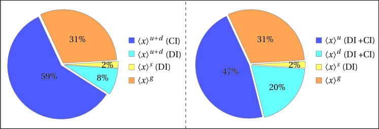
Figure 8: Preliminary results for the quark and gluon contributions to the proton momentum, presented at Lattice 2013. Courtesy of Keh-Fei Liu.

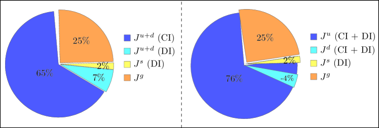
Figure 9: Preliminary results for the quark and gluon contributions to the angular momentum, presented at Lattice 2013. Courtesy of Keh-Fei Liu.

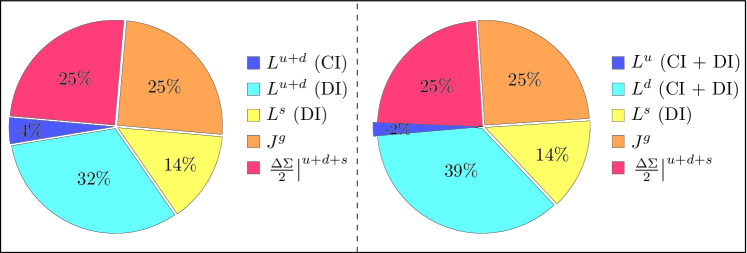
Figure 10: Preliminary results for the quark and gluon contributions to the orbital angular momentum, presented at Lattice 2013. Courtesy of Keh-Fei Liu.

These figures give very interesting information as to how the proton spin is built up, in the Ji decomposition, from the contributions of its constituents. The values for the orbital angular momentum given here should be compared with the model calculations labeled $\ell^{q}_{\text{kin},z}$ in Table 5 in section VII.3. However, it will be of far more fundamental interest when these numbers can be compared with the experimentally measured GPDs appearing in the relations in sections VI.6 and VIII.3.

VII.1.2 Lattice calculation of $J^{q}_{\text{Bel},T}$

It should be noted that once $A_{q}$ and $B_{q}$ or, equivalently $T_{1}(0)_{q}$ and $T_{2}(0)_{q}$, have been evaluated from lattice studies of the longitudinal case, the Leader relation given by Eq. (360) for the transverse case can be used as a test of the consistency of the theory. Thus a direct evaluation on a lattice of

$$J_{q,T}\equiv\langle\langle P,\mathscr{S}_{T}|J^{q}_{\text{Bel},T}|P,\mathscr{S}_{T}\rangle\rangle$$ (441)

for a transversely polarized proton moving with a few different values of momentum, could be compared with the expected behavior

$$J_{q,T}=\tfrac{1}{2}\left(A_{q}+\tfrac{P^{0}}{M}\,B_{q}\right).$$ (442)

VII.1.3 Evaluation of $L^{q}_{\text{Ji},z}$ in a longitudinally polarized nucleon, from GPDs

We shall now show how the light-front version of $L^{q}_{\text{Ji},z}$ can be related to the twist-3 GPDs defined according to the parametrization of Kiptily and Polyakov Kiptily:2002nx , namely

$$\frac{1}{2}\int\frac{\mathrm{d}z^{-}}{2\pi}\,e^{ix\bar{P}^{+}z^{-}}\langle P^{\prime},\mathscr{S}^{\prime}|\overline{\psi}(-\tfrac{z^{-}}{2})\gamma^{j}\mathcal{W}\psi(\tfrac{z^{-}}{2})|P,\mathscr{S}\rangle\\ =\frac{1}{2\bar{P}^{+}}\,\overline{u}(P^{\prime},\mathscr{S}^{\prime})\left[\frac{\Delta^{j}_{\perp}}{2M}\,G^{q}_{1}+\gamma^{j}\left(H_{q}+E_{q}+G^{q}_{2}\right)+\frac{\Delta^{j}_{\perp}\gamma^{+}}{\bar{P}^{+}}\,G^{q}_{3}+\frac{i\epsilon^{jk}_{T}\Delta^{k}_{\perp}\gamma^{+}\gamma_{5}}{\bar{P}^{+}}\,G^{q}_{4}\right]u(P,\mathscr{S}),$$ (443)

where the nucleon is moving in the $z$-direction, $\bm{\Delta}_{\perp}$ is the transverse part of $\Delta^{\mu}$, and the indices $j,k=1,2$ are transverse indices. Analogously to Eq. (340), if we multiply by $x$ and integrate, one obtains

$$\langle P^{\prime},\mathscr{S}^{\prime}|\tfrac{1}{2}\,\overline{\psi}(0)\gamma^{j}i\overset{\leftrightarrow}{D}\!\!\!\!\!\phantom{D}^{+}\psi(0)|P,\mathscr{S}\rangle =\bar{P}^{+}\,\overline{u}(P^{\prime},\mathscr{S}^{\prime})\left[\frac{\Delta^{j}_{\perp}}{2M}\int\mathrm{d}x\,x\,G^{q}_{1}+\gamma^{j}\int\mathrm{d}x\,x\left(H_{q}+E_{q}+G^{q}_{2}\right)\right.$$

$$\qquad\qquad\qquad\qquad+\left.\frac{\Delta^{j}_{\perp}\gamma^{+}}{\bar{P}^{+}}\int\mathrm{d}x\,x\,G^{q}_{3}+\frac{i\epsilon^{jk}_{T}\Delta^{k}_{\perp}\gamma^{+}\gamma_{5}}{\bar{P}^{+}}\int\mathrm{d}x\,x\,G^{q}_{4}\right]u(P,\mathscr{S}).$$ (444)

Now analogously to Eq. (VI.6), one can write for $\mu\neq\nu$,

$$\langle P^{\prime},\mathscr{S}^{\prime}|\tfrac{1}{2}\,\overline{\psi}(0)\gamma^{\mu}i\overset{\leftrightarrow}{D}\!\!\!\!\!\phantom{D}^{\nu}\psi(0)|P,\mathscr{S}\rangle =\overline{u}(P^{\prime},\mathscr{S}^{\prime})\left[\frac{\bar{P}^{\{\mu}\gamma^{\nu\}}}{2}\,A_{q}(\Delta^{2})+\frac{\bar{P}^{\{\mu}i\sigma^{\nu\}\rho}\Delta_{\rho}}{4M}\,B_{q}(\Delta^{2})\right.$$

$$\left.+\frac{\Delta^{\mu}\Delta^{\nu}-\Delta^{2}g^{\mu\nu}}{M}\,C_{q}(\Delta^{2})+Mg^{\mu\nu}\bar{C}_{q}(\Delta^{2})+\frac{\bar{P}^{[\mu}\gamma^{\nu]}}{2}\,D_{q}(\Delta^{2})\right]u(P,\mathscr{S}),$$ (445)

with the notations $a^{\{\mu}b^{\nu\}}=a^{\mu}b^{\nu}+a^{\nu}b^{\mu}$ and $a^{[\mu}b^{\nu]}=a^{\mu}b^{\nu}-a^{\nu}b^{\mu}$. Remembering that $\bar{P}^{\mu}=[\bar{P}^{+},\bar{P}^{-},\bm{0}_{\perp}]$, one obtains for $\mu=j$, $\nu=+$

$$\langle P^{\prime},\mathscr{S}^{\prime}|\tfrac{1}{2}\,\overline{\psi}(0)\gamma^{j}i\overset{\leftrightarrow}{D}\!\!\!\!\!\phantom{D}^{+}\psi(0)|P,\mathscr{S}\rangle=\overline{u}(P^{\prime},\mathscr{S}^{\prime})\left\{\frac{\gamma^{j}\bar{P}^{+}}{2}\left[A_{q}(\Delta^{2})+B_{q}(\Delta^{2})-D_{q}(\Delta^{2})\right]+\frac{\Delta^{+}\Delta^{j}}{M}\,C_{q}(\Delta^{2})\right\}u(P,\mathscr{S}),$$ (446)

where we have used $\overline{u}^{\prime}\frac{i\sigma^{j\rho}\Delta_{\rho}}{2M}\,u=\overline{u}^{\prime}\gamma^{j}u$. Comparing with Eq. (VII.1.3) and taking the limit $\Delta^{\mu}\rightarrow 0$, we see that

$$\int\mathrm{d}x\,x\,\left[H_{q}(x,0,0)+E_{q}(x,0,0)+G^{q}_{2}(x,0,0)\right]=\tfrac{1}{2}\left(A_{q}+B_{q}-D_{q}\right),$$ (447)

so that

$$-\int\mathrm{d}x\,x\,G^{q}_{2}(x,0,0)=\langle\langle P,\mathscr{S}_{L}|J^{q}_{\text{Bel},z}|P,\mathscr{S}_{L}\rangle\rangle+\tfrac{1}{2}\,D_{q}.$$ (448)

Consider now the expression for the orbital angular momentum. From Eq. (132)

$$\langle P,\mathscr{S}_{L}|L^{q}_{\text{Ji},z}|P,\mathscr{S}_{L}\rangle=\langle P,\mathscr{S}_{L}|\int\mathrm{d}x^{-}\mathrm{d}^{2}x_{\perp}\left[\tfrac{1}{2}\,\overline{\psi}(0)\gamma^{+}x^{1}i\overset{\leftrightarrow}{D}\!\!\!\!\!\phantom{D}^{2}\psi(0)-(1\leftrightarrow 2)\right]|P,\mathscr{S}_{L}\rangle,$$ (449)

so that analogously to Eq. (319) we will have

$$\langle\langle P,\mathscr{S}_{L}|L^{q}_{\text{Bel},z}|P,\mathscr{S}_{L}\rangle\rangle=\frac{1}{2P^{+}}\left[-i\,\frac{\partial}{\partial\Delta^{1}}\langle P+\tfrac{\Delta}{2},\mathscr{S}_{Lf}|\tfrac{1}{2}\,\overline{\psi}(0)\gamma^{+}i\overset{\leftrightarrow}{D}\!\!\!\!\!\phantom{D}^{2}\psi(0)|P-\tfrac{\Delta}{2},\mathscr{S}_{Li}\rangle-(1\leftrightarrow 2)\right]_{\bm{\Delta}=\bm{0}},$$ (450)

where we have allowed for the fact that for light-front states are normalized so that

$$\langle P^{\prime}|P\rangle=2P^{+}\,(2\pi)^{3}\,\delta(P^{\prime+}-P^{+})\,\delta^{(2)}(\bm{P}^{\prime}_{\perp}-\bm{P}_{\perp}).$$ (451)

Using the expression in Eq. (430) for the matrix elements on the RHS of Eq. (450) together with Eq. (346), yields

$$\langle\langle P,\mathscr{S}_{L}|L^{q}_{\text{Ji},z}|P,\mathscr{S}_{L}\rangle\rangle =\tfrac{1}{2}\left(A_{q}+B_{q}+D_{q}\right)$$

$$=\langle\langle P,\mathscr{S}_{L}|J^{q}_{\text{Bel},z}|P,\mathscr{S}_{L}\rangle\rangle+\tfrac{1}{2}\,D_{q},$$ (452)

so that

$$-\tfrac{1}{2}\,D_{q}=\tfrac{1}{2}\,a^{q}_{0}=\langle\langle P,\mathscr{S}_{L}|S^{q}_{z}|P,\mathscr{S}_{L}\rangle\rangle.$$ (453)

Substituting in Eq. (448) yields an expression for the orbital angular momentum

$$\langle\langle P,\mathscr{S}_{L}|L^{q}_{\text{Ji},z}|P,\mathscr{S}_{L}\rangle\rangle=-\int_{-1}^{1}\mathrm{d}x\,x\,G^{q}_{2}(x,0,0).$$ (454)

Note that one gets exactly the same expression for the $z$ component of the instant form orbital angular momentum. This relation was first obtained by Penttinen, Polyakov, Shuvaev and Strikman in the parton model Penttinen:2000dg and later confirmed in QCD by Hatta and Yoshida Hatta:2012cs .

One has therefore the following genuine and non-trivial sum rule

$$\int_{-1}^{1}\mathrm{d}x\,x\left[H_{q}(x,0,0)+E_{q}(x,0,0)+2G^{q}_{2}(x,0,0)\right]-a^{q}_{0}=0.$$ (455)

The relation between twist-3 GPDs and the kinetic orbital angular momentum has also been discussed by Ji, Xiong and Yuan Ji:2012ba , and similar expressions can be found in the gluon sector Hatta:2012cs ; Ji:2012ba . Unfortunately, it will be very difficult to extract the twist-3 GPD $G_{2}$ accurately from experiment.

VII.1.4 Evaluation of $L^{q}_{\text{Ji},z}$ in a longitudinally polarized nucleon, from GTMDs

Another possibility to learn about the orbital angular momentum consists in considering twist-2 generalized transverse-momentum dependent distributions (GTMDs), also called unintegrated or $k_{\perp}$-dependent GPDs, defined as Meissner:2009ww

$$\frac{1}{2}\int\frac{\mathrm{d}z^{-}\,\mathrm{d}^{2}z_{\perp}}{(2\pi)^{3}}\,e^{ix\bar{P}^{+}z^{-}-i\bm{k}_{\perp}\cdot\bm{z}_{\perp}}\langle P^{\prime},\mathscr{S}^{\prime}|\overline{\psi}(-\tfrac{z}{2})\gamma^{+}\mathcal{W}\psi(\tfrac{z}{2})|P,\mathscr{S}\rangle\big{|}_{z^{+}=0}\\ =\frac{1}{2M}\,\overline{u}(P^{\prime},\mathscr{S}^{\prime})\left[F^{q}_{1,1}+\frac{i\sigma^{j+}k^{j}_{\perp}}{\bar{P}^{+}}\,F^{q}_{1,2}+\frac{i\sigma^{j+}\Delta^{j}_{\perp}}{\bar{P}^{+}}\,F^{q}_{1,3}+\frac{i\sigma^{jk}k^{j}_{\perp}\Delta^{k}_{\perp}}{M^{2}}\,F^{q}_{1,4}\right]u(P,\mathscr{S}),$$ (456)

where $j,k=1,2$ are transverse indices. The GTMDs are functions of the quark momentum $(x\bar{P}^{+},\bm{k}_{\perp})$ and the momentum transfer $\Delta$, and depend upon the choice made for the Wilson line $\mathcal{W}$. For vanishing skewness $\xi=0$, their Fourier transform from $\bm{\Delta}_{\perp}$-space to $\bm{b}_{\perp}$-space can be interpreted as relativistic phase-space or Wigner distributions Lorce:2011kd

$$\rho^{q}_{\mathscr{S}^{\prime}\mathscr{S}}(x,\bm{k}_{\perp},\bm{b}_{\perp};\mathcal{W})=\int\frac{\mathrm{d}^{2}\Delta_{\perp}}{(2\pi)^{2}}\,e^{-i\bm{\Delta}_{\perp}\cdot\bm{b}_{\perp}}\,\frac{1}{2}\int\frac{\mathrm{d}z^{-}\,\mathrm{d}^{2}z_{\perp}}{(2\pi)^{3}}\,e^{ix\bar{P}^{+}z^{-}-i\bm{k}_{\perp}\cdot\bm{z}_{\perp}}\,\langle P^{\prime},\mathscr{S}^{\prime}|\overline{\psi}(-\tfrac{z}{2})\gamma^{+}\mathcal{W}\psi(\tfrac{z}{2})|P,\mathscr{S}\rangle\big{|}_{z^{+}=0}.$$ (457)

It can be shown that the longitudinal component of the Ji quark orbital angular momentum can be written as Lorce:2011kd ; Lorce:2011ni

$$\langle\langle P,\mathscr{S}_{L}|L^{q}_{\text{Ji},z}|P,\mathscr{S}_{L}\rangle\rangle =\int\mathrm{d}x\,\mathrm{d}^{2}k_{\perp}\,\mathrm{d}^{2}b_{\perp}\left(\bm{b}_{\perp}\times\bm{k}_{\perp}\right)_{z}\,\rho^{q}_{\mathscr{S}_{L}\mathscr{S}_{L}}(x,\bm{k}_{\perp},\bm{b}_{\perp};\mathcal{W}_{\text{straight}})$$

$$=-\int\mathrm{d}x\,\mathrm{d}^{2}k_{\perp}\,\frac{\bm{k}^{2}_{\perp}}{M^{2}}\,F^{q}_{1,4}(x,\bm{k}_{\perp},\Delta=0;\mathcal{W}_{\text{straight}}),$$ (458)

where the Wilson line $\mathcal{W}_{\text{straight}}$ connects the points $-\tfrac{z}{2}$ and $\tfrac{z}{2}$ by a direct straight line Ji:2012sj ; Lorce:2012ce . One has therefore the following non-trivial sum rule

$$\int_{-1}^{1}\mathrm{d}x\left[x\left[H_{q}(x,0,0)+E_{q}(x,0,0)\right]-2\int\mathrm{d}^{2}k_{\perp}\,\frac{\bm{k}^{2}_{\perp}}{M^{2}}\,F^{q}_{1,4}(x,\bm{k}_{\perp},0;\mathcal{W}_{\textrm{straight}})\right]-a^{q}_{0}=0.$$ (459)

Note that, unfortunately, at present there is no clear way of extracting the twist-2 GTMDs from experimental data. This sum rule can therefore be only tested in lattice and model calculations.

VII.2 Expressions for the canonical version of $\bm{L}$

It is extremely interesting that the gauge-invariant canonical orbital angular momentum $L^{q}_{\text{gic},z}$, which equals the Jaffe-Manohar orbital angular momentum evaluated in the gauge $A^{+}=0$, i.e. $L^{q}_{\text{JM},z}|_{A^{+}=0}$, can be expressed in terms of the same twist-2 GTMD, but defined with a different choice of Wilson line Lorce:2011kd ; Lorce:2011ni . One obtains

$$\langle\langle P,\mathscr{S}_{L}|L^{q}_{\text{gic},z}|P,\mathscr{S}_{L}\rangle\rangle=-\int\mathrm{d}x\,\mathrm{d}^{2}k_{\perp}\,\frac{\bm{k}^{2}_{\perp}}{M^{2}}\,F^{q}_{1,4}(x,\bm{k}_{\perp},\Delta=0;\mathcal{W}_{\textrm{LF}}),$$ (460)

where the staple-like Wilson line $\mathcal{W}_{\textrm{LF}}$ connects the points $-\tfrac{z}{2}$ and $\tfrac{z}{2}$ via the intermediary points $-\tfrac{z}{2}+\eta\infty^{-}$ and $\tfrac{z}{2}+\eta\infty^{-}$ by straight lines, with the parameter $\eta$ indicating whether the Wilson lines are future pointing ($\eta=+1$) or past pointing ($\eta=-1$) Meissner:2009ww . In the light-front gauge, this Wilson line reduces to a transverse straight link at light-front infinity $x^{-}=\eta\infty^{-}$. Because of parity and time-reversal symmetry, this residual gauge link does not contribute to the orbital angular momentum in the light-front gauge and can simply be ignored Hatta:2011ku ; Hatta:2012cs ; Ji:2012ba ; Lorce:2012ce .

So, by merely changing the shape of the Wilson line, one obtains either the kinetic or the canonical quark orbital angular momentum Ji:2012sj ; Lorce:2012ce . Hatta showed that a similar expression holds in the gluon sector Hatta:2011ku . For a complete parametrization of the gluon GTMDs, see Ref. Lorce:2013pza . The gauge-invariant canonical orbital angular momentum can also be accessed via twist-3 GPDs by adding the potential angular momentum $L_{\text{pot},z}$ discussed in section V.2.3 to the kinetic, i.e. Ji, orbital angular momentum. Explicit, but cumbersome, expressions have been given in Refs. Hatta:2012cs ; Ji:2012ba .

In lattice calculations, it is technically very difficult to fix a gauge. One is therefore forced to make calculations including explicitly the Wilson line. Note that very interesting pioneer calculations of naive T-odd TMDs on a lattice with staple-like Wilson lines have been carried out in Ref. Musch:2011er . Moreover, Ji proposed a new strategy for computing parton distributions, in leading twist, on a lattice using space-like operators instead of light-like operators Ji:2013dva , the former being more amenable to a lattice implementation than the latter. Because of these encouraging developments, we believe it is reasonable to expect the first lattice evaluations of the canonical orbital angular momentum (460) within the coming years.

VII.3 The orbital angular momentum in quark models

Quark models are usually based on approximate or phenomenological expressions for the quark wave function inside a nucleon. Knowing this wave function, one has in principle all the information needed for computing the quark orbital angular momentum. Since gluons are absent in quark models, model results are commonly thought to be approximations of QCD at very low scale and in a fixed gauge, usually taken to be the light-front gauge $A^{+}=0$, to make contact with the partonic picture. Like in most studies, we shall consider only the longitudinal component of the quark orbital angular momentum

$$\ell^{q}_{z}\equiv\langle\langle P,\mathscr{S}_{L}|L^{q}_{z}|P,\mathscr{S}_{L}\rangle\rangle.$$ (461)

The quark kinetic (or Ji) orbital angular momentum can be obtained in a model by calculating the GPDs involved in the Ji relation

$$\ell^{q}_{\text{kin},z}=\tfrac{1}{2}\int^{1}_{-1}\mathrm{d}x\left\{x\left[H_{q}(x,0,0)+E_{q}(x,0,0)\right]-\tilde{H}_{q}(x,0,0)\right\},$$ (462)

where $\tilde{H}$ is the helicity GPD satisfying

$$\int\mathrm{d}x\,\tilde{H}_{q}(x,0,0)=a^{q}_{0}.$$ (463)

In principle, one should get the same result from the twist-3 GPD relation (454)

$$\ell^{q}_{\text{kin},z}=-\int_{-1}^{1}\mathrm{d}x\,x\,G^{q}_{2}(x,0,0),$$ (464)

and the GTMD relation (458)

$$\ell^{q}_{\text{kin},z}=-\int\mathrm{d}x\,\mathrm{d}^{2}k_{\perp}\,\frac{\bm{k}^{2}_{\perp}}{M^{2}}\,F^{q}_{1,4}(x,\bm{k}_{\perp},\Delta=0;\mathcal{W}_{straight})$$ (465)

with a straight Wilson line. In practice, the last two approaches are often problematic and, to the best of our knowledge, the equivalence has never been checked explicitly in model calculations so far. The reason is that twist-3 GPDs contain interaction which is often missing or hard to compute realistically in quark models. Note also that the twist-3 GPD relation (464) is based on the QCD equations of motion which usually differ from the model equations of motion. Concerning the GTMD relation with straight Wilson lines, one cannot get rid of the straight Wilson line when $k_{\perp}\neq 0$, by keeping the same choice of gauge at each spatial point Lorce:2012ce , so one cannot avoid the inclusion of gluons.

The quark canonical (or Jaffe-Manohar) orbital angular momentum can be calculated by means of the GTMD relation (460)

$$\ell^{q}_{\text{can},z}=-\int\mathrm{d}x\,\mathrm{d}^{2}k_{\perp}\,\frac{\bm{k}^{2}_{\perp}}{M^{2}}\,F^{q}_{1,4}(x,\bm{k}_{\perp},\Delta=0;\mathcal{W}_{\text{LF}}),$$ (466)

where the staple-like Wilson line $\mathcal{W}_{\text{LF}}$ can basically be ignored in the light-front gauge, as explained earlier. This orbital angular momentum coincides with the partonic orbital angular momentum calculated in terms of light-front wave functions Lorce:2011ni ; Lorce:2011kn

$$\ell^{q}_{\text{can},z}=\sum_{n}\sum_{\{\lambda\}}\sum_{l,r(q)}(\delta_{rl}-x_{l})\int[\mathrm{d}x]_{n}\,[\mathrm{d}^{2}k_{\perp}]_{n}\,\Psi^{*+}_{n}(\{x,\bm{k}_{\perp},\lambda\})\left(\bm{k}_{r\perp}\times\tfrac{1}{i}\bm{\nabla}_{\bm{k}_{l\perp}}\right)_{z}\Psi^{+}_{n}(\{x,\bm{k}_{\perp},\lambda\}),$$ (467)

defined with respect to the transverse center of momentum Burkardt:2000za ; Burkardt:2002hr

$$\bm{R}_{\perp}=\sum^{n}_{l=1}x_{l}\,\bm{r}_{l\perp},$$ (468)

where in momentum space $\bm{r}_{l\perp}=\tfrac{1}{i}\bm{\nabla}_{\bm{k}_{l\perp}}$. In Eq. (467), $\Psi^{\Lambda}_{n}$ is the $n$-parton light-front wave function for a nucleon with polarization $\Lambda$. The argument $\{x,\bm{k}_{\perp},\lambda\}$ stands for the set of parton longitudinal momentum fractions, transverse momenta and polarizations, and the integration measures read

$$[\mathrm{d}x]_{n}\equiv\left[\prod_{l=1}^{n}\mathrm{d}x_{l}\right]\delta\!\left(1-\sum^{n}_{l=1}x_{l}\right),\qquad[\mathrm{d}^{2}k_{\perp}]_{n}\equiv\left[\prod_{l=1}^{n}\frac{\mathrm{d}^{2}k_{l\perp}}{2(2\pi)^{3}}\right]2(2\pi)^{3}\,\delta^{(2)}\!\left(\sum^{n}_{l=1}\bm{k}_{l\perp}\right).$$ (469)

Similarly to section VI.7.2, $r(q)$ means that the sum is restricted to those values of $r$ corresponding to quarks of flavor $q$.

In quark model calculations, like e.g. Ma:1998ar , one often defines the canonical orbital angular momentum with respect to the coordinate axes, so that

$$\mathcal{L}^{q}_{\text{can},z}=\sum_{n}\sum_{\{\lambda\}}\sum_{r(q)}\int[\mathrm{d}x]_{n}\,[\mathrm{d}^{2}k_{\perp}]_{n}\,\Psi^{*+}_{n}(\{x,\bm{k}_{\perp},\lambda\})\left(\bm{k}_{r\perp}\times\tfrac{1}{i}\bm{\nabla}_{\bm{k}_{r\perp}}\right)_{z}\Psi^{+}_{n}(\{x,\bm{k}_{\perp},\lambda\}).$$ (470)

This expression is somewhat simpler than Eq. (469) and comes from the fact that the transverse position of the nucleon is not properly taken into account. So, Eq. (470) represents the naive canonical orbital angular momentum, while Eq. (469) represents the intrinsic canonical orbital angular momentum Lorce:2011kn . However, when summing over all the partons, the difference between naive and intrinsic orbital angular momentum disappears. In Ref. Brodsky:2000ii , it is stressed that, owing to the momentum conservation constraint, there can only be $n-1$ relative orbital angular momentum contributions in a $n$-parton Fock state. Note, however, that there is no unique way to define such $n-1$ relative constributions for $n>2$. Moreover, one cannot unambiguously attribute a given contribution to a particular parton. The transverse center of momentum provides the additional point with respect to which one can define unambiguously $n$ intrinsic contributions, each associated with a particular parton. Some quark-model calculations Ma:1998ar ; She:2009jq ; Avakian:2010br suggested that the naive quark canonical orbital angular momentum defined in Eq. (470) may be related to the so-called pretzelosity transverse-momentum dependent distribution (TMD) $h_{1T}^{\perp}$ as follows

$$\mathcal{L}^{q}_{\text{can},z}=-\int\mathrm{d}x\,\mathrm{d}^{2}k_{\perp}\,\frac{\bm{k}_{\perp}^{2}}{2M^{2}}\,h_{1T}^{\perp q}(x,\bm{k}^{2}_{\perp}).$$ (471)

It appeared, unfortunately, that such a relation is only valid in a restricted class of models Lorce:2011dv ; Lorce:2011kn , where the instant-form wave function $\psi(\{\bm{k},\sigma\})$ is a pure $s$-wave and related to the light-front wave function $\Psi(\{x,\bm{k}_{\perp},\lambda\})$ by a mere Wigner rotation, which allows one to write canonical spin $\sigma$ in terms of light-front helicity $\lambda$

$$\Psi(\{x,\bm{k}_{\perp},\lambda\})=\psi(\{\bm{k},\sigma\})\prod_{l}D_{\lambda_{l}\sigma_{l}}(x_{l},\bm{k}_{l\perp}),\qquad D_{\lambda\sigma}(x,\bm{k}_{\perp})=\begin{pmatrix}\cos\tfrac{\theta}{2}&\hat{k}_{L}\sin\tfrac{\theta}{2}\\ -\hat{k}_{R}\sin\tfrac{\theta}{2}&\cos\tfrac{\theta}{2}\end{pmatrix},$$ (472)

with $\hat{k}_{R,L}=(k^{1}\pm ik^{2})/|\bm{k}_{\perp}|$ and $\theta\equiv\theta(x,\bm{k}_{\perp})$ a function of the quark momentum specific to the model. In this class of models, all the orbital angular momentum in the light-front wave function is simply generated by this Wigner rotation. Indeed, using the light-front wave function in Eq. (472), the naive canonical orbital angular momentum given by Eq. (470) reads

$$\mathcal{L}^{q}_{\text{can},z}=\sum_{n}\sum_{\{\sigma\}}\sum_{r(q)}\int[\mathrm{d}x]_{n}\,[\mathrm{d}^{2}k_{\perp}]_{n}\left|\psi^{+}_{n}(\{\bm{k},\sigma\})\right|^{2}\left(1-\cos\theta_{r}\right)\sigma_{r},$$ (473)

where $\theta_{r}\equiv\theta(x_{r},\bm{k}_{r\perp})$ and $\sigma_{r}=\pm 1/2$. The same Wigner rotation is responsible for the existence of a non-vanishing pretzelosity TMD $h_{1T}^{\perp}$. Using the generic results of Ref. Lorce:2011zta , one can write in the restricted class of models

$$\frac{\bm{k}_{\perp}^{2}}{2M^{2}}\,h_{1T}^{\perp q}(x,\bm{k}^{2}_{\perp})=\sum_{n}\sum_{\{\sigma\}}\sum_{r(q)}\int[\mathrm{d}x]_{n}\,[\mathrm{d}^{2}k_{\perp}]_{n}\left|\psi^{+}_{n}(\{\bm{k},\sigma\})\right|^{2}\delta(x-x_{r})\,\delta^{(2)}(\bm{k}_{\perp}-\bm{k}_{r\perp})\left(\cos\theta_{r}-1\right)\sigma_{r}$$ (474)

where the pure $s$-wave nature of the instant-form wave function was crucial in the intermediate steps. Comparing Eqs. (473) and (474), one obtains the model-dependent relation (471) and understands it as originating from a pure Wigner rotation effect. The same effect is at the origin other relations among TMDs observed in the restricted class of models Lorce:2011zta .

In Table 5, we reproduce the results for the three versions of orbital angular momentum given by Eqs. (462), (466) and (471) within the light-front constituent quark model (LFCQM) and the light-front chiral quark-soliton model (LF$\chi$QSM) restricted to the three-quark sector Lorce:2011kd . In these models, Eq. (471) coincides with the naive definition of quark canonical orbital angular momentum (470).

Table 5: Comparison between the kinetic ($\ell^{q}_{\text{kin},z}$), intrinsic canonical ($\ell^{q}_{\text{can},z}$) and naive canonical ($\mathcal{L}^{q}_{\text{can},z}$) orbital angular momentum in the light-front constituent quark model (LFCQM) and the light-front chiral quark-soliton model (LF$\chi$QSM) for $u$-, $d$- and total ($u+d$) quark contributions.

Model	LFCQM			LF$\chi$QSM
$q$	$u$	$d$	Total	$u$	$d$	Total
$\ell^{q}_{\text{kin},z}$	$0.071$	$~{}~{}0.055$	$0.126$	$-0.008$	$~{}~{}0.077$	$0.069$
$\ell^{q}_{\text{can},z}$	$0.131$	$-0.005$	$0.126$	$~{}~{}0.073$	$-0.004$	$0.069$
$\mathcal{L}^{q}_{\text{can},z}$	$0.169$	$-0.042$	$0.126$	$~{}~{}0.093$	$-0.023$	$0.069$

As expected in a pure quark model, all three versions of “$\ell$” in each model give the same value for the total orbital angular momentum, but widely different results between the models. However, differences between the various definitions appear in the separate quark-flavor contributions. The difference between the naive and intrinsic canonical orbital angular momentum naturally comes from the fact that the individual orbital angular momentum contributions are not defined with respect to the same point. What is more surprising is that $\ell^{q}_{\text{kin},z}\neq\ell^{q}_{\text{can},z}$, since it is generally believed that the kinetic and canonical orbital angular momentum should coincide in absence of gluons. Note that a similar observation has also been made in the instant-form version of the $\chi$QSM Wakamatsu:2005vk , where the Ji relation (462) was shown not to hold for the isovector combination $u-d$ in the model. This should actually not be so surprising, since the Ji relation is obtained using the QCD expression for the energy-momentum tensor, and not the quark model expression. Only in some cases, like e.g. in the scalar diquark model Burkardt:2008ua , one obtains $\ell^{q}_{\text{kin},z}=\ell^{q}_{\text{can},z}$. A comparison between the kinetic and canonical orbital angular momentum, where the gauge potential is included, can be found in Refs. Burkardt:2008ua ; Burkardt:2010he . For a physical interpretation of the difference $\ell^{q}_{\text{kin},z}-\ell^{q}_{\text{can},z}$, see Ref. Burkardt:2012sd .

VII.4 The phase-space distribution of angular momentum

We have essentially discussed the angular momentum integrated over all phase space. It is however possible to define densities of angular momentum as well. Many definitions have been proposed in the literature, creating a lot of confusion. One of the reasons is that different densities can lead to the same integrated quantity, a long as they differ by superpotential terms. The archetypical example is the total angular momentum of the system, which can be obtained either from the canonical density or the Belinfante-improved density. In the first case, the angular momentum density is naturally decomposed into an orbital angular momentum density and a spin density. In the second case, the spin density is converted into an orbital angular momentum density by adding a superpotential. It is therefore essential to keep track of these superpotential terms.

Since the $t$ dependence of twist-2 GPDs contains, via two-dimensional Fourier transform, the information about the spatial distribution of partons Burkardt:2000za ; Burkardt:2002hr , it has been suggested by Goeke et al. Goeke:2007fp that the Ji relation generalized to $t\neq 0$ contains the information about the spatial distribution of Belinfante angular momentum

$$J_{q}(t)=\tfrac{1}{2}\int\mathrm{d}x\,x\left[H_{q}(x,0,t)+E_{q}(x,0,t)\right].$$ (475)

It has also been suggested in Refs. Hoodbhoy:1998yb ; Ji:2012sj ; Ji:2012ba that the integrand of the Ji relation

$$J_{q}(x)=\tfrac{x}{2}\left[H_{q}(x,0,0)+E_{q}(x,0,0)\right]$$ (476)

can be interpreted as the density of angular momentum in $x$-space. In the scalar diquark model, where it is straightforward to maintain Lorentz invariance and where the absence of the gauge potential allows one to identify Ji and Jaffe-Manohar orbital angular momentum, Burkardt and Hikmat Burkardt:2008ua checked that

$$\int\mathrm{d}x\,J_{q}(x)=\int\mathrm{d}x\,L_{q}(x)+\int\mathrm{d}x\,S_{q}(x),$$ (477)

but observed that

$$J_{q}(x)\neq L_{q}(x)+S_{q}(x),$$ (478)

where $J_{q}(x)$, $L_{q}(x)$ and $S_{q}(x)$ are the angular momentum, orbital angular momentum and spin densities

$$J_{q}(x) =\tfrac{x}{2}\int\frac{\mathrm{d}^{2}k_{\perp}}{2(2\pi)^{3}}\left[\left|\psi^{+}_{+}(x,\bm{k}_{\perp})\right|^{2}+\left|\psi^{+}_{-}(x,\bm{k}_{\perp})\right|^{2}-2M\,\psi^{+*}_{+}(x,\bm{k}_{\perp})\,\tfrac{\partial}{\partial\Delta^{1}}\psi^{-}_{+}(x,\bm{k}_{\perp}-(1-x)\bm{\Delta}_{\perp})\big{|}_{\bm{\Delta}_{\perp}=\bm{0}_{\perp}}\right],$$ (479)

$$L_{q}(x) =\int\frac{\mathrm{d}^{2}k_{\perp}}{2(2\pi)^{3}}\,(1-x)\left|\psi^{+}_{-}(x,\bm{k}_{\perp})\right|^{2},$$ (480)

$$S_{q}(x) =\tfrac{1}{2}\int\frac{\mathrm{d}^{2}k_{\perp}}{2(2\pi)^{3}}\left[\left|\psi^{+}_{+}(x,\bm{k}_{\perp})\right|^{2}-\left|\psi^{+}_{-}(x,\bm{k}_{\perp})\right|^{2}\right],$$ (481)

expressed in terms of the light-front wave function $\psi^{\Lambda}_{\lambda}(x,\bm{k}_{\perp})$ of the scalar diquark model. The lack of equality in (478) caused much puzzlement, since it seems difficult to understand. It cannot be explained by the extra contribution obtained by Hoodbhoy, Ji and Lu Hoodbhoy:1998yb , since the latter is proportional to the gluon field strength $G^{\mu\nu}$, and therefore cannot contribute in the scalar diquark model. Upon examination, it turns out that belief in the equality of the LHS and RHS of (478) is based on a paper of Hoodbhoy, Ji and Lu who actually showed that for the Mellin moments, defined as $f_{n}\equiv\int\mathrm{d}x\,x^{n-1}f(x)$, one has

$$J_{qn}=L_{qn}+S_{qn},$$ (482)

provided one drops systematically the surface terms for each $n$. In other words, they implicitly assumed that all the Mellin moments of the superpotential term vanish, implying that the superpotential itself vanishes, which is impossible for a particle with spin. Similarly, Adhikari and Burkardt Adhikari:2013ima checked in the same scalar diquark model that

$$\int\mathrm{d}^{2}b_{\perp}\,J_{q}(\bm{b}_{\perp})=\int\mathrm{d}^{2}b_{\perp}\,L_{q}(\bm{b}_{\perp})+\int\mathrm{d}^{2}b_{\perp}\,S_{q}(\bm{b}_{\perp}),$$ (483)

but observed that

$$J_{q}(\bm{b}_{\perp})\neq L_{q}(\bm{b}_{\perp})+S_{q}(\bm{b}_{\perp}),$$ (484)

where for $\xi=0$

$$f(\bm{b}_{\perp})\equiv\int\frac{\mathrm{d}^{2}\Delta_{\perp}}{(2\pi)^{2}}\,e^{-i\bm{\Delta}_{\perp}\cdot\bm{b}_{\perp}}\,f(t=-\bm{\Delta}^{2}_{\perp}).$$ (485)

We note that the actual spatial density of angular momentum receives a contribution from the Fourier transform of both $J_{q}(t)$ and $t\,\tfrac{\partial}{\partial t}J_{q}(t)$. The second term does not contribute to the total angular momentum since the integral over all space amounts to set $t=0$. Nevertheless, even with the correct spatial density associated with $J_{q}(t)$, we expect the non-equality Eq. (484) to remain true. Indeed, the contribution from the superpotential term to the spatial density cannot identically vanish if the spin density does not identically vanish as well.

The most natural definition of angular momentum density is based on phase-space distributions, also known as Wigner distributions. In the context of QCD, non-relativistic expressions have been introduced and discussed in Refs. Ji:2003ak ; Belitsky:2003nz . The corresponding relativistic expressions have been written down and studied by Lorcé and Pasquini in Ref. Lorce:2011kd . They defined the relativistic quark phase-space density in a longitudinally polarized nucleon as

$$\rho^{q}(x,\bm{k}_{\perp},\bm{b}_{\perp};\mathcal{W})=\int\frac{\mathrm{d}^{2}\Delta_{\perp}}{(2\pi)^{2}}\,e^{-i\bm{\Delta}_{\perp}\cdot\bm{b}_{\perp}}\,\frac{1}{2}\int\frac{\mathrm{d}z^{-}\mathrm{d}^{2}z_{\perp}}{(2\pi)^{3}}\,e^{ik\cdot z}\,\langle P^{+},\tfrac{\bm{\Delta}_{\perp}}{2},\mathscr{S}_{L}|\overline{\psi}(-\tfrac{z}{2})\gamma^{+}\mathcal{W}\psi(\tfrac{z}{2})|P^{+},-\tfrac{\bm{\Delta}_{\perp}}{2},\mathscr{S}_{L}\rangle\big{|}_{z^{+}=0},$$ (486)

where the parametrization of the GTMD correlator is given by Eq. (456). Note that, using the light-front spinors, only the $F_{1,1}$ and $F_{1,4}$ GTMDs contribute in the case of longitudinal polarization. We can then write

$$\rho^{q}(x,\bm{k}_{\perp},\bm{b}_{\perp};\mathcal{W})=\mathcal{F}^{q}_{1,1}(x,\bm{k}^{2}_{\perp},\bm{k}_{\perp}\cdot\bm{b}_{\perp},\bm{b}^{2}_{\perp};\mathcal{W})-\tfrac{1}{M^{2}}\,\left(\bm{k}_{\perp}\times\bm{\nabla}_{\bm{b}_{\perp}}\right)_{z}\mathcal{F}^{q}_{1,4}(x,\bm{k}^{2}_{\perp},\bm{k}_{\perp}\cdot\bm{b}_{\perp},\bm{b}^{2}_{\perp};\mathcal{W}),$$ (487)

where

$$\mathcal{F}^{q}_{1,i}(x,\bm{k}^{2}_{\perp},\bm{k}_{\perp}\cdot\bm{b}_{\perp},\bm{b}^{2}_{\perp};\mathcal{W})=\int\frac{\mathrm{d}^{2}\Delta_{\perp}}{(2\pi)^{2}}\,e^{-i\bm{\Delta}_{\perp}\cdot\bm{b}_{\perp}}\,F^{q}_{1,i}(x,\xi=0,\bm{k}^{2}_{\perp},\bm{k}_{\perp}\cdot\bm{\Delta}_{\perp},\bm{\Delta}^{2}_{\perp};\mathcal{W})$$ (488)

for $i=1,4$. The density of total longitudinal orbital angular momentum Lorce:2011kd ; Lorce:2011ni can then naturally be defined as

$$L^{q}_{z}(x,\bm{k}_{\perp},\bm{b}_{\perp};\mathcal{W})=\left(\bm{b}_{\perp}\times\bm{k}_{\perp}\right)_{z}\,\rho^{q}(x,\bm{k}_{\perp},\bm{b}_{\perp};\mathcal{W}).$$ (489)

Like in the integrated case, for a staple-like Wilson line in the light-front direction, it coincides with the canonical or Jaffe-Manohar orbital angular momentum in the light-front gauge

$$L^{q}_{\text{can},z}(x,\bm{k}_{\perp},\bm{b}_{\perp})=L^{q}_{z}(x,\bm{k}_{\perp},\bm{b}_{\perp};\mathcal{W}_{\text{LF}}).$$ (490)

For a straight Wilson line, as explained by Lorcé in Ref. Lorce:2012ce , it is necessary to integrate over $\bm{k}_{\perp}$ to interpret it as the kinetic (or Ji) orbital angular momentum. So we have

$$L^{q}_{\text{kin},z}(x,\bm{b}_{\perp})=\int\mathrm{d}^{2}k_{\perp}\,L^{q}_{z}(x,\bm{k}_{\perp},\bm{b}_{\perp};\mathcal{W}_{\text{straight}}).$$ (491)

From the quark phase-space distribution, one can also define in a natural way the distribution of average quark (canonical) transverse momentum in impact-parameter space as

$$\langle\bm{k}^{q}_{\perp}\rangle(\bm{b}_{\perp})=\int\mathrm{d}x\,\mathrm{d}^{2}k_{\perp}\,\bm{k}_{\perp}\,\rho^{q}(x,\bm{k}_{\perp},\bm{b}_{\perp};\mathcal{W}_{\text{LF}}).$$ (492)

The longitudinal component of the quark canonical orbital angular momentum in impact-parameter space then reads

$$L^{q}_{\text{can},z} =\int\mathrm{d}^{2}b_{\perp}\left[\bm{b}_{\perp}\times\langle\bm{k}^{q}_{\perp}\rangle(\bm{b}_{\perp})\right]_{z}$$

$$=-\int\mathrm{d}x\,\mathrm{d}^{2}k_{\perp}\,\mathrm{d}^{2}b_{\perp}\,\frac{\bm{k}^{2}_{\perp}}{M^{2}}\,\mathcal{F}^{q}_{1,4}(x,\bm{k}^{2}_{\perp},\bm{k}_{\perp}\cdot\bm{b}_{\perp},\bm{b}^{2}_{\perp};\mathcal{W}_{\text{LF}})$$

$$=-\int\mathrm{d}x\,\mathrm{d}^{2}k_{\perp}\,\frac{\bm{k}^{2}_{\perp}}{M^{2}}\,F^{q}_{1,4}(x,0,\bm{k}^{2}_{\perp},0,0;\mathcal{W}_{\text{LF}}).$$ (493)

The distribution of average quark transverse momentum has been computed within the LFCQM in Ref. Lorce:2011ni . In Fig. 11, we show the same distribution, obtained this time within the LF$\chi$QSM.

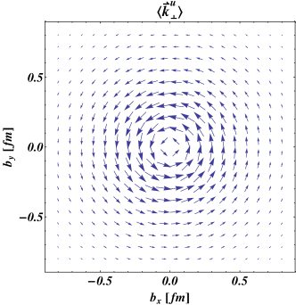
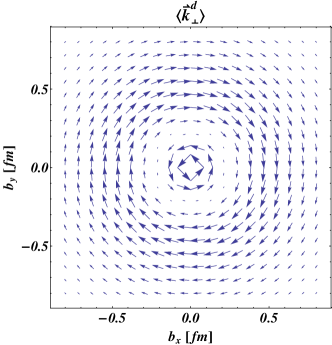
Figure 11: Distributions in impact-parameter space of the average transverse momentum of up quarks (left panel) and down quarks (right panel) in a longitudinally polarized nucleon, computed within the light-front chiral quark-soliton model (LF$\chi$QSM). The nucleon polarization is pointing out of the plane, and the arrows show the size and direction of the average quark transverse momentum.

It clearly shows that in a longitudinally polarized nucleon, the quarks have on average nonzero orbital angular momentum. From Eq. (487), it is clear that the polar component, and hence the average orbital angular momentum, originates solely from the $F_{1,4}$ GTMD. In principle, there can also be a radial component. From parity, time-reversal and hermiticity constraints, the latter can only receive contributions from the imaginary part of the GTMDs representing the effect of initial and final state interactions Meissner:2009ww . Such interactions being absent in the model, no radial contribution was obtained.

VIII Qualitative summary and experimental implications

In this section, we summarize the essential points concerning the issue of angular momentum decomposition and the experimental implications.

VIII.1 Gauge invariance and measurability

Gauge-invariant quantities are in principle measurable, whereas gauge non-invariant quantities are often claimed to be not measurable. It turns out, however, that gauge non-invariant quantities considered in some chosen gauge can in principle also be measured. One way of understanding this is that there always exists a non-local gauge-invariant quantity (called gauge-invariant extension) that gives the same numerical answer as a local gauge non-invariant quantity in the chosen gauge. The archetypical example is the quantity called $\Delta G$. It is a measurable quantity whose gauge-invariant expression is clearly non-local. Only in the light-front gauge does this expression reduce to the local expression for the gluon spin contribution given by Jaffe and Manohar. So measuring $\Delta G$ is the same as obtaining the value of the gluon spin in the gauge $A^{+}=0$.

It is therefore essential to separate two things: the measured quantity and its physical interpretation. A measured quantity is necessarily gauge independent, but its interpretation need not be. This is nicely stated by Bashinsky and Jaffe: “one should make clear what a quark or a gluon parton is in an interacting theory. The subtlety here is the issue of gauge invariance: a pure quark field in one gauge is a superposition of quarks and gluons in another. Different ways of gluon-field gauge fixing predetermine different decompositions of the coupled quark-gluon fields into quark and gluon degrees of freedom.” Analogously, in particle physics one measures the four-momentum squared of a particle, which is a Lorentz-invariant quantity, but its physical interpretation as the mass squared of the particle is valid only in the rest frame.

The parton model is a picture of the nucleon in the infinite momentum frame, i.e. in a frame where the nucleon moves with almost the speed of light. This picture is particularly useful to understand what is going on in scattering experiments involving high momentum transfer, like e.g. deep-inelastic scattering, and predates QCD. The light-front gauge is particularly appealing in the infinite-momentum frame, since it relegates dynamical aspects to kinematically suppressed contributions. For this reason, the parton model picture is commonly identified with QCD in the light-front gauge and in the infinite-momentum frame (or equivalently at leading twist). Strictly speaking, the light-front gauge is not more “physical” than any other gauge, but turns out to be more convenient for the interpretation of high-energy scattering experiments. One could of course choose to work in a different gauge, but the price to pay is high: far more complicated expressions and totally unclear physical interpretation.

The approach proposed a few years ago by Chen et al. Chen:2008ag reopened hordes of old controversies. But after many subsequent papers and discussions, one should recognize that nothing really new has appeared from the practical/experimental point of view. The new developments concern the physical interpretation point of view. Thus, the Chen et al. approach provides a concrete non-local gauge-invariant alternative to the former local gauge non-invariant interpretation. In particular, it makes it clearer why a gauge non-invariant quantity in some chosen gauge can actually be “measured”. It is therefore possible to interpret in any gauge $\Delta G$ as the gluon spin contribution, provided that the latter is re-defined in a non-local way.

In summary, our opinion is that there is no fundamental reason for insisting that the physical interpretation of a measurable quantity be gauge and/or frame independent. The important question is to determine whether a gauge non-invariant quantity with clear physical interpretation can be associated with a measurable quantity. Formally, this is always possible, since it suffices to write down the corresponding non-local gauge-invariant extension. The problematic but crucial point is actually to find a way of extracting the latter from experimental data. Since the nucleon internal structure is essentially probed in the infinite-momentum frame, the only experimentally relevant non-local gauge-invariant quantities are those defined with Wilson lines running essentially along the light-front direction.

VIII.2 Two kinds of decompositions

There are fundamentally two kinds of proton angular momentum decomposition:

• The canonical decomposition is based on Noether’s theorem and is written in terms of canonical generators of rotation. It is essentially the Jaffe-Manohar decomposition Jaffe:1989jz , which has to be thought of in the light-front gauge in order to make contact with actual experiments. This decomposition can be rewritten in a gauge-invariant but non-local way, as shown explicitly by Hatta Hatta:2011ku .

• The kinetic decomposition is based on the gauge-invariant Belinfante-improved energy-momentum tensor. The form used by Ji Ji:1996ek consists of three gauge-invariant local contributions (quark spin, quark orbital angular momentum and gluon total angular momentum) and is obtained using the QCD equations of motion and discarding surface terms. By either fixing a gauge or considering non-local expressions, the gluon total angular momentum can further be split into spin and orbital angular momentum contributions, as discussed by Wakamatsu Wakamatsu:2010qj .

Opinions diverge as to which kind of decomposition should be considered as “the” physical one. Both canonical and kinetic decompositions can in principle be accessed experimentally. It turns out that the canonical decomposition provides a clearer partonic interpretation, while the kinetic decomposition is easier to access experimentally. In our opinion, both are interesting.

By either fixing a gauge or working with non-local gauge-invariant expressions, the nucleon angular momentum can actually be decomposed into five contributions, instead of the naively expected four. Beside quark spin, quark orbital angular momentum, gluon spin and gluon orbital angular momentum, there is a so-called potential angular momentum Wakamatsu:2010qj . The canonical and kinetic decompositions simply differ in the attribution of this term to either quarks or gluons. The potential term is particularly interesting, as suggested by Burkardt Burkardt:2012sd , since it is somehow related to the torque that acts on a quark in longitudinally polarized DIS. So, in some sense, the canonical and kinetic decompositions can be viewed as two different groupings of terms belonging to a single more general decomposition.

VIII.3 Sum rules vs. relations

It is important to keep in mind the difference between a sum rule and a relation:

• A sum rule is an identity between measurable quantities. An identity involves only objects that transform in the same manner under gauge and Lorentz transformations, and so is valid in any gauge and in any Lorentz frame. If experiment shows that such a sum rule does not hold, it implies a failure of the theory.

• A relation allows one to evaluate a theoretical quantity, itself not directly measurable from experiment, using the values of other measurable quantities. The interpretation is generally valid only in a fixed (or a restricted class of) gauge and/or Lorentz frame. Using a relation does not directly test a theory, though it might be used to test a model or lattice calculation of the theoretical quantity.

Prior to defining angular momentum, one has first to specify what form of dynamics one is working in, since instant form and light-front form operators usually differ, as explained in section II.2.3. Similarly, one has also to specify what kind of definition for spin one is using in a moving frame (canonical spin, helicity, light-front helicity, etc.). While a sum rule is insensitive to these choices, the particular quantity studied in a relation will in general depend on them. However, if one considers a relation in the infinite-momentum frame (or, equivalently, restricts it to its leading-twist part), these particular choices usually do not matter.

While there are few genuine sum rules, many relations have appeared recently and caused a lot of confusion. In the following, we list the most relevant ones in connection with the angular momentum decomposition. For convenience, we always choose the spatial axes such that the nucleon momentum lies along the $OZ$ axis, i.e. we can write $P^{\mu}=(P^{0},0,0,P_{z})$ without loss of generality. We use the notation

$$\langle\langle P,\mathscr{S}|O|P,\mathscr{S}\rangle\rangle=\frac{\langle P,\mathscr{S}|O|P,\mathscr{S}\rangle}{\langle P,\mathscr{S}|P,\mathscr{S}\rangle}$$ (494)

for the expectation value of an operator $O$, and work in the $\overline{MS}$ scheme.

VIII.3.1 Sum rules

As shown in section VI, the nucleon matrix elements of the quark and gluon energy-momentum density are expressed in terms of form factors $A_{i}(t)$, $B_{i}(t)$, $C_{i}(t)$ and $\bar{C}_{i}(t)$, where $t=\Delta^{2}$ is the invariant momentum transfer and the index $i$ labels specific quarks or gluons. Momentum conservation then implies the momentum sum rule

$$\sum_{q,G}A_{i}(0)=1.$$ (495)

From conservation of total angular momentum, one obtains the angular momentum sum rule

$$\sum_{q,G}\tfrac{1}{2}\left[A_{i}(0)+B_{i}(0)\right]=\tfrac{1}{2}.$$ (496)

Combining momentum and angular momentum sum rules leads to the so-called anomalous gravitomagnetic moment sum rule

$$\sum_{q,G}B_{i}(0)=0,$$ (497)

which can be shown to imply that the nucleon anomalous gravitomagnetic moment vanishes Brodsky:2000ii ; Teryaev:1999su . The $\bar{C}$ form factors appear only in the non-conserved individual quark and gluon energy-momentum tensors, so one has also the following sum rule

$$\sum_{q,G}\bar{C}_{i}(t)=0,$$ (498)

which is valid for any $t$.

The $A$ and $B$ form factors can be expressed in terms of the second $x$-moment of the twist-2 GPDs $H$ and $E$ Ji:1996ek ; Diehl:2003ny

$$A_{q,G}(t)=\int\mathrm{d}x\,x\,H_{q,G}(x,0,t),\qquad B_{q,G}(t)=\int\mathrm{d}x\,x\,E_{q,G}(x,0,t),$$ (499)

where $q$ refers to the sum of quark and antiquark of a given flavor. Integrals over quark GPDs run from $-1$ to $+1$, whereas integrals over gluon GPDs run from $0$ to $1$. For the $\bar{C}$ quark form factor, we find

$$\bar{C}_{q}(t)=\int\mathrm{d}x\,x\left[H^{q}_{3}(x,0,t)-\tfrac{1}{2}\,H_{q}(x,0,t)\right],$$ (500)

where $H_{3}$ is a twist-four GPD. A similar expression is expected to hold in the gluon sector. Plugging these GPD expressions in the sum rules (495), (497) and (498), one arrives at

$$\sum_{q,G}\int\mathrm{d}x\,x\,H_{i}(x,0,0) =1,$$ (501)

$$\sum_{q,G}\int\mathrm{d}x\,x\,E_{i}(x,0,0) =0,$$ (502)

$$\sum_{q,G}\int\mathrm{d}x\,x\,H^{i}_{3}(x,0,t) =\tfrac{1}{2}\sum_{q,G}\int\mathrm{d}x\,x\,H_{i}(x,0,t).$$ (503)

In addition, there is the Penttinen-Polyakov-Shuvaev-Strikman sum rule Penttinen:2000dg ; Hatta:2012cs derived in section VII.1.3, which, in the parametrization of Kiptily and Polyakov for twist-3 GPDs Kiptily:2002nx , reads

$$\int\mathrm{d}x\,x\left[H_{q}(x,0,0)+E_{q}(x,0,0)+2G^{q}_{2}(x,0,0)\right]=\int\mathrm{d}x\,\tilde{H}_{q}(x,0,0),$$ (504)

where $G_{2}$ is a genuine twist-3 GPD and where one can write

$$\int\mathrm{d}x\,\tilde{H}_{q}(x,0,0)=a^{q}_{0},$$ (505)

with $a^{q}_{0}$ the contribution of a quark plus antiquark of a given flavor to the nucleon flavor singlet axial charge $a_{0}$ (or $g_{A}^{(0)}$).

We stress that the above are genuine sum rules in that all the quantities they contain can, at least in principle, be determined from experiment. Of course, extracting them from experiment may be extremely difficult in practice. Finally, one can also write the following sum rule

$$\int\mathrm{d}x\,G^{q}_{2}(x,0,0)=\int\mathrm{d}x\,\mathrm{d}^{2}k_{\perp}\,\frac{\bm{k}^{2}_{\perp}}{M^{2}}\,F^{q}_{1,4}(x,\bm{k}_{\perp},0;\mathcal{W}_{\text{straight}}),$$ (506)

which is unfortunately not relevant from the experimental point of view, since there is no indication so far as to how one can extract this particular GTMD, especially since it has a Wilson line that does not run along the light-front direction. The best chance to check this sum rule is therefore with model and lattice calculations.

VIII.3.2 Instant form relations

In instant form, as explained in section II.2.3, the operator $Q$ associated with any density $j^{\mu}$ is defined as

$$Q=\int\mathrm{d}^{3}x\,j^{0}(x),$$ (507)

and the covariant spin four-vector is given by

$$\mathscr{S}^{\mu}(P,\bm{s})=(P_{z}s_{z},M\bm{s}_{\perp},P^{0}s_{z}).$$ (508)

The nucleon state normalization reads

$$\langle P,\mathscr{S}|P,\mathscr{S}\rangle=2P^{0}\,(2\pi)^{3}\,\delta^{(3)}(\bm{0}).$$ (509)

Focusing on the longitudinal component of the angular momentum in a longitudinally polarized nucleon, one has the following explicit kinetic decompositions:

• the Belinfante decomposition

  $$\tfrac{1}{2}=\sum_{q}\langle\langle P,\mathscr{S}_{L}|J^{q}_{\text{Bel},z}|P,\mathscr{S}_{L}\rangle\rangle+\langle\langle P,\mathscr{S}_{L}|J^{G}_{\text{Bel},z}|P,\mathscr{S}_{L}\rangle\rangle,$$ (510)

• the Ji decomposition

  $$\tfrac{1}{2}=\sum_{q}\langle\langle P,\mathscr{S}_{L}|S^{q}_{z}|P,\mathscr{S}_{L}\rangle\rangle+\sum_{q}\langle\langle P,\mathscr{S}_{L}|L^{q}_{\text{Ji},z}|P,\mathscr{S}_{L}\rangle\rangle+\langle\langle P,\mathscr{S}_{L}|J^{G}_{\text{Bel},z}|P,\mathscr{S}_{L}\rangle\rangle,$$ (511)

where the various contributions are given explicitly in the following. Note that no explicit canonical decomposition is available in the instant form, unless one considers the infinite-momentum frame where instant and light-front forms simply coincide. For this reason, the explicit canonical decompositions will be considered only in the next subsection where the light-front expressions are discussed. In the following relations the first line of each equation involves quantities, form factors, that can be measured on a lattice, and the further lines involve experimentally measurable quantities.

The longitudinal component of the kinetic angular momentum carried by quarks and gluons is related to experimentally measurable quantities by the Ji relation Ji:1996ek

$$\begin{split}\langle\langle P,\mathscr{S}_{L}|J^{i}_{\text{Bel},z}|P,\mathscr{S}_{L}\rangle\rangle\equiv\langle\langle P,\mathscr{S}_{L}|M^{12}_{\text{Bel},i}|P,\mathscr{S}_{L}\rangle\rangle&=\tfrac{1}{2}\left[A_{i}(0)+B_{i}(0)\right]\\ &=\tfrac{1}{2}\int\mathrm{d}x\,x\left[H_{i}(x,0,0)+E_{i}(x,0,0)\right],\end{split}$$ (512)

with $i=q,G$ and $\mathscr{S}_{L}\equiv\mathscr{S}(P,\bm{e}_{z})$.

The quark longitudinal spin is given by

$$\begin{split}\langle\langle P,\mathscr{S}_{L}|S^{q}_{z}|P,\mathscr{S}_{L}\rangle\rangle\equiv\langle\langle P,\mathscr{S}_{L}|M^{12}_{q,\text{spin}}|P,\mathscr{S}_{L}\rangle\rangle&=\tfrac{1}{2}\,a^{q}_{0}\\ &=\tfrac{1}{2}\int\mathrm{d}x\,\tilde{H}_{q}(x,0,0).\end{split}$$ (513)

This relation does not depend on the magnitude of the nucleon momentum, and remains therefore valid in the infinite-momentum frame $P_{z}\to\infty$. In this frame, the quarks move essentially collinearly with the nucleon, and so one can identify the quark longitudinal spin with the quark helicity.

Finally, there are several relations with experimental quantities for the longitudinal component of the quark kinetic orbital angular momentum Penttinen:2000dg ; Ji:2012sj ; Lorce:2012ce

$$\begin{split}\langle\langle P,\mathscr{S}_{L}|L^{q}_{\text{Ji},z}|P,\mathscr{S}_{L}\rangle\rangle\equiv\langle\langle P,\mathscr{S}_{L}|M^{12}_{\text{Ji},q,\text{OAM}}|P,\mathscr{S}_{L}\rangle\rangle&=\tfrac{1}{2}\left[A_{q}(0)+B_{q}(0)-a^{q}_{0}\right]\\ &=\tfrac{1}{2}\int\mathrm{d}x\,x\left[H_{q}(x,0,0)+E_{q}(x,0,0)\right]-\tfrac{1}{2}\int\mathrm{d}x\,\tilde{H}_{q}(x,0,0)\\ &=-\int\mathrm{d}x\,x\,G^{q}_{2}(x,0,0)\\ &=-\int\mathrm{d}x\,\mathrm{d}^{2}k_{\perp}\,\frac{\bm{k}^{2}_{\perp}}{M^{2}}\,F^{q}_{1,4}(x,\bm{k}_{\perp},0;\mathcal{W}_{\text{straight}}).\end{split}$$ (514)

Turning now to the transverse component of the kinetic angular momentum in a transversely polarized nucleon, say in the $x$-direction, there is the Leader relation Leader:2011cr

$$\begin{split}\langle\langle P,\mathscr{S}_{x}|J^{i}_{\text{Bel},x}|P,\mathscr{S}_{x}\rangle\rangle\equiv\langle\langle P,\mathscr{S}_{x}|M^{23}_{\text{Bel},i}|P,\mathscr{S}_{x}\rangle\rangle&=\tfrac{1}{2}\left[A_{i}(0)+\tfrac{P^{0}}{M}\,B_{i}(0)\right]\\ &=\tfrac{1}{2}\int\mathrm{d}x\,x\left[H_{i}(x,0,0)+\tfrac{P^{0}}{M}\,E_{i}(x,0,0)\right],\end{split}$$ (515)

with $i=q,G$ and $\mathscr{S}_{x}\equiv\mathscr{S}(P,\bm{e}_{x})$. Contrary to the longitudinal component, the transverse component of the kinetic angular momentum depends on the momentum of the nucleon. This should not be surprising, since longitudinal boosts commute with longitudinal rotations, but not with transverse rotations. In the rest frame $P^{0}=M$, the Ji and Leader relations naturally coincide by rotational invariance. Note also that the momentum-dependent term drops out when considering the total (i.e. quark$+$gluon) angular momentum, thanks to the anomalous gravitomagnetic sum rule (497) or equivalently (502).

To avoid momentum dependence in the case of transverse polarization, Ji, Xiong and Yuan Ji:2012vj proposed to consider instead the quark and gluon contributions to the Pauli-Lubanski four-vector of the nucleon

$$W^{\mu}_{\text{Bel},i}\equiv\tfrac{1}{2}\,\epsilon^{\mu\nu\rho\sigma}M^{\text{Bel},i}_{\nu\rho}P_{\sigma}$$ (516)

with $i=q,G$ and $\epsilon_{0123}=+1$, and $P_{\sigma}$ is the total momentum operator. The Pauli-Lubanski four-vector has the welcome feature that

$$\langle\langle P,\mathscr{S}|\sum_{q,G}W^{\mu}_{\text{Bel},i}|P,\mathscr{S}\rangle\rangle=\tfrac{1}{2}\,\mathscr{S}^{\mu}.$$ (517)

For the transverse component, say in the $x$-direction, Leader Leader:2012ar obtained

$$\begin{split}\langle\langle P,\mathscr{S}_{x}|W^{1}_{\text{Bel},i}|P,\mathscr{S}_{x}\rangle\rangle&=\tfrac{1}{2}\left[A_{i}(0)+B_{i}(0)+\tfrac{P^{0}-M}{P^{0}}\,\bar{C}_{i}(0)\right]\mathscr{S}^{1}_{x}\\ &=\tfrac{1}{2}\int\mathrm{d}x\,x\left[\tfrac{P^{0}+M}{2P^{0}}\,H_{i}(x,0,0)+E_{i}(x,0,0)+\tfrac{P^{0}-M}{P^{0}}\,H^{i}_{3}(x,0,0)\right]\mathscr{S}^{1}_{x}.\end{split}$$ (518)

So, even by using the Pauli-Lubanski four-vector for the transverse polarization, one cannot get rid of the momentum dependence for the separate quark and gluon contributions. Only for the total (i.e. quark$+$gluon) Pauli-Lubanski four-vector does the momentum dependence drop out, owing to Eq. (498) or equivalently Eq. (503). In the rest frame $P^{0}=M$, the spatial components of the Pauli-Lubanski four-vector coincide with the angular momentum operators times the nucleon mass

$$\bm{W}^{q,G}_{\text{Bel}}\big{|}_{P^{0}=M}=M\bm{J}^{q,G}_{\text{Bel}},$$ (519)

so it is quite natural that Eq. (518) agrees with the Ji (512) and Leader (515) relations in the rest frame.

VIII.3.3 Light-front form relations

In light-front form, the operator $Q$ associated with a density $j^{\mu}$ is defined as

$$Q=\int\mathrm{d}x^{-}\mathrm{d}^{2}x_{\perp}\,j^{+}(x),$$ (520)

and the covariant spin four-vector is given by

$$\mathscr{S}^{\mu}=[P^{+}s_{z},-P^{-}s_{z},M\bm{s}_{\perp}].$$ (521)

The nucleon state normalization reads

$$\langle P,\mathscr{S}|P,\mathscr{S}\rangle=2P^{+}\,(2\pi)^{3}\,\delta^{(3)}(\bm{0}).$$ (522)

In this section, all operators and states are in light-front form, but to avoid a typographical mess, we shall not attach subscripts LF to the expressions.

Focusing on the longitudinal component of the angular momentum in a longitudinally polarized nucleon, one has the following explicit kinetic decompositions:

• the Belinfante decomposition

  $$\tfrac{1}{2}=\sum_{q}\langle\langle P,\mathscr{S}_{L}|J^{q}_{\text{Bel},z}|P,\mathscr{S}_{L}\rangle\rangle+\langle\langle P,\mathscr{S}_{L}|J^{G}_{\text{Bel},z}|P,\mathscr{S}_{L}\rangle\rangle,$$ (523)

• the Ji decomposition

  $$\tfrac{1}{2}=\sum_{q}\langle\langle P,\mathscr{S}_{L}|S^{q}_{z}|P,\mathscr{S}_{L}\rangle\rangle+\sum_{q}\langle\langle P,\mathscr{S}_{L}|L^{q}_{\text{Ji},z}|P,\mathscr{S}_{L}\rangle\rangle+\langle\langle P,\mathscr{S}_{L}|J^{G}_{\text{Bel},z}|P,\mathscr{S}_{L}\rangle\rangle,$$ (524)

• the light-front gauge-invariant kinetic (gik) decomposition

  $$\tfrac{1}{2}=\sum_{q}\langle\langle P,\mathscr{S}_{L}|S^{q}_{z}|P,\mathscr{S}_{L}\rangle\rangle+\sum_{q}\langle\langle P,\mathscr{S}_{L}|L^{q}_{\text{Ji},z}|P,\mathscr{S}_{L}\rangle\rangle+\langle\langle P,\mathscr{S}_{L}|S^{G}_{z}|P,\mathscr{S}_{L}\rangle\rangle+\langle\langle P,\mathscr{S}_{L}|L^{G}_{\text{gik},z}|P,\mathscr{S}_{L}\rangle\rangle,$$ (525)

and the following explicit canonical decomposition:

• the light-front gauge-invariant canonical (gic) decomposition

  $$\tfrac{1}{2}=\sum_{q}\langle\langle P,\mathscr{S}_{L}|S^{q}_{z}|P,\mathscr{S}_{L}\rangle\rangle+\sum_{q}\langle\langle P,\mathscr{S}_{L}|L^{q}_{\text{gic},z}|P,\mathscr{S}_{L}\rangle\rangle+\langle\langle P,\mathscr{S}_{L}|S^{G}_{z}|P,\mathscr{S}_{L}\rangle\rangle+\langle\langle P,\mathscr{S}_{L}|L^{G}_{\text{gic},z}|P,\mathscr{S}_{L}\rangle\rangle,$$ (526)

where the various contributions are given explicitly in the following. Note that the light-front gauge-invariant canonical decomposition was written explicitly for the first time by Hatta Hatta:2011ku and gives the same result as the Jaffe-Manohar decomposition Jaffe:1989jz in the light-front gauge $A^{+}=0$.

The longitudinal component of the kinetic angular momentum is provided once again by the Ji relation Ji:1996ek

$$\begin{split}\langle\langle P,\mathscr{S}_{L}|J^{i}_{\text{Bel},z}|P,\mathscr{S}_{L}\rangle\rangle\equiv\langle\langle P,\mathscr{S}_{L}|M^{12}_{\text{Bel},i}|P,\mathscr{S}_{L}\rangle\rangle&=\tfrac{1}{2}\left[A_{i}(0)+B_{i}(0)\right]\\ &=\tfrac{1}{2}\int\mathrm{d}x\,x\left[H_{i}(x,0,0)+E_{i}(x,0,0)\right],\end{split}$$ (527)

with $i=q,G$ and $\mathscr{S}_{L}\equiv\mathscr{S}(P,\bm{e}_{z})$.

The quark light-front helicity is given, as in Eq. (513), by

$$\begin{split}\langle\langle P,\mathscr{S}_{L}|S^{q}_{z}|P,\mathscr{S}_{L}\rangle\rangle\equiv\langle\langle P,\mathscr{S}|M^{12}_{q,\text{spin}}|P,\mathscr{S}\rangle\rangle&=\tfrac{1}{2}\,a^{q}_{0}\\ &=\tfrac{1}{2}\int\mathrm{d}x\,\tilde{H}_{q}(x,0,0).\end{split}$$ (528)

Similarly, the gluon light-front helicity is given by

$$\langle\langle P,\mathscr{S}_{L}|S^{G}_{z}|P,\mathscr{S}_{L}\rangle\rangle\equiv\langle\langle P,\mathscr{S}|M^{12}_{G,\text{spin}}|P,\mathscr{S}\rangle\rangle=\int\mathrm{d}x\,\tilde{H}_{G}(x,0,0),$$ (529)

where $M^{12}_{G,\text{spin}}$ stands, equivalently, for the local Jaffe-Manohar operator in the light-front gauge Jaffe:1989jz or the non-local gauge-invariant Hatta operator Hatta:2011zs .

The longitudinal component of the kinetic orbital angular momentum for quarks Penttinen:2000dg ; Ji:2012sj ; Lorce:2012ce reads

$$\begin{split}\langle\langle P,\mathscr{S}_{L}|L^{q}_{\text{Ji},z}|P,\mathscr{S}_{L}\rangle\rangle\equiv\langle\langle P,\mathscr{S}|M^{12}_{\text{Ji},q,\text{OAM}}|P,\mathscr{S}\rangle\rangle&=\tfrac{1}{2}\left[A_{q}(0)+B_{q}(0)-a^{q}_{0}\right]\\ &=\tfrac{1}{2}\int\mathrm{d}x\,x\left[H_{q}(x,0,0)+E_{q}(x,0,0)\right]-\tfrac{1}{2}\int\mathrm{d}x\,\tilde{H}_{q}(x,0,0)\\ &=-\int\mathrm{d}x\,x\,G^{q}_{2}(x,0,0)\\ &=-\int\mathrm{d}x\,\mathrm{d}^{2}k_{\perp}\,\frac{\bm{k}^{2}_{\perp}}{M^{2}}\,F^{q}_{1,4}(x,\bm{k}_{\perp},0;\mathcal{W}_{\text{straight}}),\end{split}$$ (530)

and similarly for gluons

$$\begin{split}\langle\langle P,\mathscr{S}_{L}|L^{G}_{\text{gik},z}|P,\mathscr{S}_{L}\rangle\rangle\equiv\langle\langle P,\mathscr{S}|M^{12}_{\text{gik},G,\text{OAM}}|P,\mathscr{S}\rangle\rangle&=\tfrac{1}{2}\int\mathrm{d}x\,x\left[H_{G}(x,0,0)+E_{G}(x,0,0)\right]-\int\mathrm{d}x\tilde{H}_{G}(x,0,0)\\ &=-\int\mathrm{d}x\,\mathrm{d}^{2}k_{\perp}\,\frac{\bm{k}^{2}_{\perp}}{M^{2}}\,F^{G}_{1,4}(x,\bm{k}_{\perp},0;\mathcal{W}_{\text{straight}}).\end{split}$$ (531)

Finally, the relation for the longitudinal component of the canonical orbital angular momentum has been obtained by Lorcé and Pasquini Lorce:2011kd for quarks, and by Hatta Hatta:2011ku for gluons

$$\langle\langle P,\mathscr{S}_{L}|L^{i}_{\text{gic},z}|P,\mathscr{S}_{L}\rangle\rangle\equiv\langle\langle P,\mathscr{S}|M^{12}_{\text{gic},i,\text{OAM}}|P,\mathscr{S}\rangle\rangle=-\int\mathrm{d}x\,\mathrm{d}^{2}k_{\perp}\,\frac{\bm{k}^{2}_{\perp}}{M^{2}}\,F^{i}_{1,4}(x,\bm{k}_{\perp},0;\mathcal{W}_{\text{staple}}),$$ (532)

where $M^{12}_{i,\text{OAM}}$ stands, equivalently, for the local Jaffe-Manohar operator in the light-front gauge Jaffe:1989jz or the non-local gauge-invariant Hatta operator Hatta:2011zs .

Turning to the transverse component of the kinetic “angular momentum” in a transversely polarized nucleon, say in the $x$-direction, one finds

$$\begin{split}\langle\langle P,\mathscr{S}_{x}|M^{-2}_{\text{Bel},i}|P,\mathscr{S}_{x}\rangle\rangle&=\tfrac{M}{2P^{+}}\left[A_{i}(0)+\tfrac{1}{2}\,B_{i}(0)+\bar{C}_{i}(0)\right]\\ &=\tfrac{M}{4P^{+}}\int\mathrm{d}x\,x\left[H_{i}(x,0,0)+E_{i}(x,0,0)+2H^{i}_{3}(x,0,0)\right],\end{split}$$ (533)

with $i=q,G$ and $\mathscr{S}_{x}\equiv\mathscr{S}(P,\bm{e}_{x})$. Contrary to the longitudinal component, the transverse component of the kinetic angular momentum depends on the momentum of the nucleon, owing to the fact that longitudinal boosts commute with longitudinal rotations, but not with transverse rotations. Note however that, contrary to the instant form, the expressions for the longitudinal and transverse components do not coincide in the rest frame $P^{+}=M$. This comes from the fact that the generators of transverse rotations are dynamical (i.e. contain interaction) in light-front form, whereas they are kinematic in instant form. The dynamical nature of the light-front generators of transverse rotations is manifested by the global $\tfrac{M}{P^{+}}$ factor indicating higher-twist, and by the presence of the $\bar{C}$ form factor. Note also that the momentum dependence does not drop out when considering the total (i.e. quark$+$gluon) generators of transverse rotations: one gets $\tfrac{M}{2P^{+}}$ instead of $\tfrac{1}{2}$. There is actually nothing wrong with that. It simply signals that the light-front generators of transverse rotations cannot be interpreted as actual angular momentum operators. Indeed, these operators satisfy the algebra of two-dimensional Euclidean space

$$\left[M^{-1},M^{-2}\right]=0,\qquad\left[M^{12},M^{-i}\right]=i\epsilon^{ij}_{\perp}M^{-j},$$ (534)

instead of the ordinary angular momentum commutation relations.

Using the Pauli-Lubanski four-vector to describe the transverse polarization, Harindranath, Kundu and Mukherjee Harindranath:2013goa obtained

$$\begin{split}\langle\langle P,\mathscr{S}_{x}|W^{1}_{\text{Bel},i}|P,\mathscr{S}_{x}\rangle\rangle&=\tfrac{1}{2}\left[A_{i}(0)+B_{i}(0)+\bar{C}_{i}(0)\right]\mathscr{S}^{1}_{x}\\ &=\tfrac{1}{2}\int\mathrm{d}x\,x\left[\tfrac{1}{2}\,H_{i}(x,0,0)+E_{i}(x,0,0)+H^{i}_{3}(x,0,0)\right]\mathscr{S}^{1}_{x},\end{split}$$ (535)

where $\mathscr{S}^{1}_{x}=M$. This is the momentum-independent relation for the transverse component of the Pauli-Lubanski four-vector. Note that the $\bar{C}$ form factor was incorrectly discarded by Ji, Xiong and Yuan Ji:2012vj . Only for the total (i.e. quark$+$gluon) Pauli-Lubanski four-vector, it is justified to do so, owing to Eq. (498) or equivalently Eq. (503).

In summary, in all the relations in this and the previous subsection, the LHS of the relations cannot be measured directly from experiment, and the RHSs simply provide information about the quantities on the LHS from experiment. The relations are thus not sum rules. However, the relations become particularly interesting when, as is sometimes possible, the LHSs can be calculated on a lattice or in models.

IX Conclusions

The desire to find an expression for the photon or gluon total angular momentum, which contains separate, gauge-invariant spin and orbital pieces has led to an outpouring of papers showing how this can be done, in, it turns out, an infinite number of different ways. None of these contradicts the age old textbook statement that this is impossible, since all the new constructions involve non-local fields, which is outside the category of local fields considered in the textbooks. A somewhat surprising corollary to these constructions is that there are an infinite number of ways to define what we mean by the quark or gluon momentum and angular momentum. It seems there is no absolutely compelling reason to prefer any one particular definition, though we feel that the fundamental versions are the canonical and the Belinfante ones, since they at least involve local fields, and it can be argued that the canonical version has certain properties that one would like to associate with an angular momentum. Moreover, they represent complementary information as to how the nucleon spin is built up from the angular momentum of its constituents, a key aspect in understanding the internal structure of the nucleon.

We have presented a pedagogical introduction to the subject and a detailed discussion of the new decompositions, and commented on their advantages and disadvantages. There have been many very interesting theoretical developments, but we have concluded that they contain no new important physical implications, and for that reason we have concentrated on experimental tests and measurements only with regard to the canonical and Belinfante versions of the angular momentum.

Because the subject is so technical we have presented a wholly pedagogical introduction and prepared a separate, largely non-technical section dealing with the physical implications. Therein we have placed particular stress on sum rules in which every term can be measured experimentally, so that a gross failure of such a sum rule would have severe implications for the validity of QCD. We have also highlighted important relations connecting some of the terms in the decompositions to experimentally measurable quantities.

References

- (1) G. Wentzel, Quantum Theory of Fields (Interscience, New York)
- (2) K. Gottfried, Quantum Mechanics (Benjamin, New York)
- (3) E. Merzbacher, Quantum Mechanics (Wiley, New York)
- (4) D. Lenstra and L. Mandel, Phys.Rev. A26, 3428 (1982)
- (5) L. Allen, M. Beijersbergen, R. Spreeuw, and J. Woerdman, Phys.Rev. A45, 8185 (1992)
- (6) S. van Enk and G. Nienhuis, Opt.Commun. 94, 147 (1992)
- (7) G. Nienhuis and L. Allen, Phys.Rev. A48, 656 (1993)
- (8) S. Barnett and L. Allen, Opt.Commun. 110, 670 (1994)
- (9) S. van Enk and G. Nienhuis, Europhys.Lett. 25, 497 (1994)
- (10) S. Barnett, J.Opt.B:Quantum Semiclass. Opt. 4, S7 (2002)
- (11) R. Jáuregui and S. Hacyan, Phys.Rev. A71, 033411 (2005)
- (12) G. Calvo, A. Picón, and E. Bagan, Phys.Rev. A73, 013805 (2006)
- (13) S. Hacyan and R. Jáuregui, J.Phys.B:At.Mol.Opt.Phys. 39, 1669 (2006)
- (14) X.-S. Chen, X.-F. Lu, W.-M. Sun, F. Wang, and T. Goldman, Phys. Rev. Lett. 100, 232002 (2008), arXiv:0806.3166 [hep-ph]
- (15) T. Nieminen, A. Stilgoe, N. Heckenberg, and H. Rubinsztein-Dunlop, J.Phys.A:Pure Appl.Opt. 10, 115005 (2008)
- (16) C. Li, Phys.Rev. A80, 063814 (2009)
- (17) M. Berry, J.Phys.A:Pure Appl.Opt. 11, 094001 (2009)
- (18) M. Mazilu, J.Phys.A:Pure Appl.Opt. 11, 094005 (2009)
- (19) A. Aiello, N. Lindlein, C. Marquardt, and G. Leuchs, Phys.Rev.Lett. 103, 100401 (2009)
- (20) A. Aiello, C. Marquardt, and G. Leuchs, Phys.Rev. A81, 053838 (2009)
- (21) S. Barnett, J.Mod.Opt. 57, 1339 (2010)
- (22) A. Stewart, Int.J.Opt. 2011, 728350 (2011), arXiv:1010.1056 [physics.class-ph]
- (23) I. Bialynicki-Birula and Z. Bialynicka-Birula, J.Opt. 13, 064014 (2011)
- (24) S. Tiwari(2008), arXiv:0807.0699 [physics.gen-ph]
- (25) X. Ji(2009), arXiv:0910.5022 [hep-ph]
- (26) X. Ji, Phys.Rev.Lett. 104, 039101 (2010)
- (27) X. Ji, Y. Xu, and Y. Zhao, JHEP 1208, 082 (2012), arXiv:1205.0156 [hep-ph]
- (28) X.-S. Chen, X.-F. Lu, W.-M. Sun, F. Wang, and T. Goldman 100, 232002 (2008), arXiv:0807.3083 [hep-ph]
- (29) X.-S. Chen, X.-F. Lu, W.-M. Sun, F. Wang, and T. Goldman(2008), arXiv:0812.4336 [hep-ph]
- (30) X.-S. Chen, W.-M. Sun, X.-F. Lu, F. Wang, and T. Goldman(2009), arXiv:0911.0248 [hep-ph]
- (31) X.-S. Chen, W.-M. Sun, F. Wang, and T. Goldman, Phys.Rev. D83, 071901 (2011), arXiv:1105.6304 [hep-ph]
- (32) C. Wong, F. Wang, W. Sun, and X. Lu(2010), arXiv:1010.4336 [hep-ph]
- (33) F. Wang, X.-S. Chen, X.-F. Lu, W.-M. Sun, and T. Goldman, Nucl.Phys. A844, 85C (2010)
- (34) X.-S. Chen, W.-M. Sun, F. Wang, and T. Goldman, Phys.Lett. B700, 21 (2011), arXiv:1101.5358 [hep-ph]
- (35) X.-S. Chen(2012), arXiv:1203.1288 [hep-ph]
- (36) T. Goldman, AIP Conf.Proc. 1418, 13 (2011), arXiv:1110.2533 [hep-ph]
- (37) M. Stoilov(2010), arXiv:1011.5617 [hep-th]
- (38) M. Wakamatsu, Phys. Rev. D81, 114010 (2010), arXiv:1004.0268 [hep-ph]
- (39) M. Wakamatsu, Phys.Rev. D83, 014012 (2011), arXiv:1007.5355 [hep-ph]
- (40) M. Wakamatsu, Phys.Rev. D84, 037501 (2011), arXiv:1104.1465 [hep-ph]
- (41) M. Wakamatsu, Phys.Rev. D85, 114039 (2012), arXiv:1204.2860 [hep-ph]
- (42) M. Wakamatsu(2013), arXiv:1302.5152 [hep-ph]
- (43) Y. Cho, M.-L. Ge, and P. Zhang, Mod.Phys.Lett. A27, 1230032 (2012), arXiv:1010.1080 [nucl-th]
- (44) Y. Cho, M.-L. Ge, D. Pak, and P. Zhang(2011), arXiv:1102.1130 [nucl-th]
- (45) Y. Hatta, Phys.Rev. D84, 041701 (2011), arXiv:1101.5989 [hep-ph]
- (46) Y. Hatta, Phys.Lett. B708, 186 (2012), arXiv:1111.3547 [hep-ph]
- (47) Y. Hatta and S. Yoshida, JHEP 1210, 080 (2012), arXiv:1207.5332 [hep-ph]
- (48) Y. Hatta, K. Tanaka, and S. Yoshida, JHEP 1302, 003 (2013), arXiv:1211.2918 [hep-ph]
- (49) P. Zhang and D. Pak, Eur.Phys.J. A48, 91 (2012), arXiv:1110.6516 [hep-ph]
- (50) E. Leader, Phys.Rev. D83, 096012 (2011), arXiv:1101.5956 [hep-ph]
- (51) C. Lorcé, Phys.Lett. B719, 185 (2013), arXiv:1210.2581 [hep-ph]
- (52) C. Lorcé, Phys.Rev. D87, 034031 (2013), arXiv:1205.6483 [hep-ph]
- (53) C. Lorcé(2013), arXiv:1302.5515 [hep-ph]
- (54) C. Lorcé(2013), arXiv:1306.0456 [hep-ph]
- (55) E. Noether, Gott.Nachr. 1918, 235 (1918), arXiv:physics/0503066 [physics]
- (56) P. A. Dirac, Proc.Roy.Soc.Lond. A117, 610 (1928)
- (57) E. Leader, Spin in particle physics (Cambridge University Press, Cambridge, UK, 2001, 2005)
- (58) L. Landau and E. Lifshitz, Classical Theory of Fields (Addison-Wesley Press, Cambridge, Mass., USA, 1951)
- (59) J. D. Bjorken and S. D. Drell, Relativistic quantum fields (Mcgraw-Hill, New York, USA, 1965)
- (60) S. Weinberg, The Quantum theory of fields. Vol. 1: Foundations (Cambridge University Press, Cambridge, U.K., 1995)
- (61) B. Lautrup, Kgl. Danske Videnskap. Selskab, Mat.-fys. Medd. 35, 1 (1967)
- (62) N. Nakanishi, Prog. Theor. Phys. 35, 1111 (1966)
- (63) T. Kugo and I. Ojima, Prog. Theor. Phys. 60, 1869 (1978)
- (64) J. C. Collins, Renormalization (Cambridge University Press, Cambridge, UK, 1984)
- (65) X.-S. Chen and F. Wang(1998), arXiv:hep-ph/9802346 [hep-ph]
- (66) P. Hoodbhoy, X.-D. Ji, and W. Lu, Phys.Rev. D59, 074010 (1999), arXiv:hep-ph/9808305 [hep-ph]
- (67) X.-S. Chen, W.-M. Sun, and F. Wang, J.Phys. G25, 2021 (1999)
- (68) W.-M. Sun, X.-S. Chen, and F. Wang, Phys.Lett. B503, 430 (2001), arXiv:hep-th/0012027 [hep-th]
- (69) F. J. Belinfante, Physica 6, 887 (1939)
- (70) L. Rosenfeld, Mém. Acad. Roy. Belg. 18, 6 (1940)
- (71) B. L. G. Bakker, E. Leader, and T. L. Trueman, Phys. Rev. D70, 114001 (2004), arXiv:hep-ph/0406139
- (72) G. M. Shore and B. E. White, Nucl. Phys. B581, 409 (2000), arXiv:hep-ph/9912341
- (73) E. Bessel-Hagen, Math. Ann. 84 (1921)
- (74) Z.-Q. Guo and I. Schmidt, Phys.Rev. D87, 114017 (2013), arXiv:1303.7210 [hep-ph]
- (75) C. Becchi, A. Rouet, and R. Stora, Annals Phys. 98, 287 (1976)
- (76) I. V. Tyutin, Lebedev Institute preprint 39 (1975)
- (77) T. Kugo and I. Ojima, Prog. Theor. Phys. Suppl. 66, 1 (1979)
- (78) R. L. Jaffe and A. Manohar, Nucl. Phys. B337, 509 (1990)
- (79) X.-S. Chen, W.-M. Sun, X.-F. Lu, F. Wang, and T. Goldman, Phys. Rev. Lett. 103, 062001 (2009), arXiv:0904.0321 [hep-ph]
- (80) C. Lorcé(2013), arXiv:1307.4323 [hep-ph]
- (81) M. Burkardt and B. C. Hikmat, Phys. Rev. D79, 071501 (2009), arXiv:0812.1605 [hep-ph]
- (82) J. Schwinger, Phys.Rev. 125, 1043 (1962)
- (83) J. S. Schwinger, Phys.Rev. 130, 402 (1963)
- (84) R. L. Arnowitt and S. Fickler, Phys.Rev. 127, 1821 (1962)
- (85) T. Goto, Prog.Theor.Phys. 36, 1283 (1966)
- (86) R. Treat, J.Math.Phys. 13, 1704 (1972)
- (87) R. P. Treat, Phys.Rev. D12, 3145 (1975)
- (88) Y. Duan and M. Ge, Sinica.Sci. 11, 1072 (1979)
- (89) Y. Duan and S.-C. Zhao, Commun.Theor.Phys. 2, 1553 (1983)
- (90) Y.-S. Duan and X.-G. Li, Commun.Theor.Phys. 29, 237 (1998)
- (91) Y.-s. Duan and P.-m. Zhang, Mod.Phys.Lett. A17, 2283 (2002), arXiv:hep-th/0212229 [hep-th]
- (92) R. Fulp and L. Norris, J.Math.Phys. 24, 1871 (1983)
- (93) T. Kashiwa and N. Tanimura(1996), arXiv:hep-th/9605207 [hep-th]
- (94) T. Kashiwa and N. Tanimura, Phys.Rev. D56, 2281 (1997), arXiv:hep-th/9612250 [hep-th]
- (95) Z.-Q. Guo and I. Schmidt, Phys.Rev. D87, 114016 (2013), arXiv:1210.2263 [hep-ph]
- (96) E. J. Konopinski, Am.J. Phys. 46(5), 499 (1978)
- (97) E. Stueckelberg, Helv.Phys.Acta 11, 225 (1938)
- (98) E. Stueckelberg, Helv.Phys.Acta 11, 299 (1938)
- (99) E. Stueckelberg, Helv.Phys.Acta 30, 209 (1957)
- (100) W. Pauli, Rev.Mod.Phys. 13, 203 (1941)
- (101) H. Ruegg and M. Ruiz-Altaba, Int.J.Mod.Phys. A19, 3265 (2004), arXiv:hep-th/0304245 [hep-th]
- (102) J. M. Jauch and F. Rohrlich, The Theory of Photons and Electrons (Addison-Wesley, Cambridge, USA, 1955)
- (103) V. Berestetskii, E. Lifshitz, and L. Pitaevskii, Quantum Electrodynamics (Pergamon, Oxford, U.K., 1982)
- (104) C. Cohen-Tannoudji, J. Dupont-Roc, and G. Grynberg, Photons and Atoms (John Wiley and Sons Inc., New York, N.Y., 1989)
- (105) S. Bashinsky and R. Jaffe, Nucl.Phys. B536, 303 (1998), arXiv:hep-ph/9804397 [hep-ph]
- (106) S. Ivanov, G. Korchemsky, and A. Radyushkin, Yad.Fiz. 44, 230 (1986)
- (107) F. J. Belinfante, Phys.Rev. 128, 2832 (1962)
- (108) S. Mandelstam, Annals Phys. 19, 1 (1962)
- (109) F. Rohrlich and F. Strocchi, Phys.Rev. 139, B476 (1965)
- (110) K. Yang, J.Phys. A18, 979 (1985)
- (111) T. Kashiwa and Y. Takahashi(1994), arXiv:hep-th/9401097 [hep-th]
- (112) T. Kashiwa and N. Tanimura, Fortsch.Phys. 45, 381 (1997)
- (113) J. Simmons and M. Guttmann, States, Waves, and Photons (Addison-Wesley, Reading, Mass., 1970)
- (114) B. S. DeWitt, Phys.Rev. 162, 1195 (1967)
- (115) B. S. DeWitt, Phys.Rev. 162, 1239 (1967)
- (116) B. S. DeWitt(1980)
- (117) G. ’t Hooft(1975)
- (118) M. T. Grisaru, P. van Nieuwenhuizen, and C. Wu, Phys.Rev. D12, 3203 (1975)
- (119) D. G. Boulware, Phys.Rev. D23, 389 (1981)
- (120) L. Abbott, Nucl.Phys. B185, 189 (1981)
- (121) G. ’t Hooft, Nucl.Phys. B62, 444 (1973)
- (122) G. ’t Hooft and M. Veltman, Annales Poincare Phys.Theor. A20, 69 (1974)
- (123) S. Deser, J. Kay, and K. Stelle, Phys.Rev.Lett. 38, 527 (1977)
- (124) L. Abbott and S. Deser, Nucl.Phys. B195, 76 (1982)
- (125) A. Petrov(2007), arXiv:0705.0019 [gr-qc]
- (126) A. N. Petrov and R. R. Lompay, Gen.Rel.Grav. 45, 545 (2013), arXiv:1211.3268 [gr-qc]
- (127) R. F. Dashen and D. J. Gross, Phys.Rev. D23, 2340 (1981)
- (128) L. Abbott and S. Deser, Phys.Lett. B116, 259 (1982)
- (129) M. Luscher and P. Weisz, Nucl.Phys. B452, 213 (1995), arXiv:hep-lat/9504006 [hep-lat]
- (130) F. Freire, D. F. Litim, and J. M. Pawlowski, Phys.Lett. B495, 256 (2000), arXiv:hep-th/0009110 [hep-th]
- (131) D. Binosi and J. Papavassiliou, Phys.Rept. 479, 1 (2009), arXiv:0909.2536 [hep-ph]
- (132) D. Binosi and A. Quadri, Phys.Rev. D85, 121702 (2012), arXiv:1203.6637 [hep-th]
- (133) L. Abbott, Acta Phys.Polon. B13, 33 (1982)
- (134) A. Guay(2004)
- (135) L. Smolin(2005), arXiv:hep-th/0507235 [hep-th]
- (136) D. Rickles, 133(2008)
- (137) M. Rozali, Adv.Sci.Lett. 2, 244 (2009), arXiv:0809.3962 [gr-qc]
- (138) M. Barenz(2012), arXiv:1207.0340 [gr-qc]
- (139) J. Collins, D. Soper, and G. Sterman, Perturbative Quantum Chromodynamics (World Scientific, Singapore)
- (140) X. Ji, J.-H. Zhang, and Y. Zhao(2013), arXiv:1304.6708 [hep-ph]
- (141) V. Gribov, Nucl.Phys. B139, 1 (1978)
- (142) R. P. Feynman, Phys.Rev.Lett. 23, 1415 (1969)
- (143) C. Rovelli(2013), arXiv:1308.5599 [hep-th]
- (144) G. P. Lepage and S. J. Brodsky, Phys.Rev. D22, 2157 (1980)
- (145) S. J. Brodsky, H.-C. Pauli, and S. S. Pinsky, Phys.Rept. 301, 299 (1998), arXiv:hep-ph/9705477 [hep-ph]
- (146) J. Jackson, Classical Electrodynamics (John Wiley & Sons, New York, USA, 1999)
- (147) R. Feynman, R. Leighton, and M. Sands, The Feynman Lectures on Physics, Vol. III (Addison-Wesley, Reading, MA, USA, 1965)
- (148) E. B. Manoukian, J.Phys. G13, 1013 (1987)
- (149) K. Moriyasu(1984)
- (150) S. R. Coleman and J. Mandula, Phys.Rev. 159, 1251 (1967)
- (151) X.-D. Ji, Phys. Rev. Lett. 78, 610 (1997), arXiv:hep-ph/9603249
- (152) D. Soper, Classical Field Theory (John Wiley and Sons, New York, USA, 1976)
- (153) P. A. Dirac, Can.J.Phys. 33, 650 (1955)
- (154) B. S. DeWitt, Phys.Rev. 125, 2189 (1962)
- (155) S. Mandelstam, Phys.Rev. 175, 1580 (1968)
- (156) S. Mandelstam, Phys.Rev. 175, 1604 (1968)
- (157) I. Bialynicki-Birula, Bull.Acad.Pol.Sci. 11, 135 (1963)
- (158) O. Steinmann, Annals Phys. 157, 232 (1984)
- (159) O. Steinmann, Helv.Phys.Acta 58, 995 (1985)
- (160) N. Skachkov, I. Solovtsov, and O. Y. Shevchenko, Z.Phys. C29, 631 (1985)
- (161) P. E. Haagensen and K. Johnson(1997), arXiv:hep-th/9702204 [hep-th]
- (162) R. Horan, M. Lavelle, and D. McMullan, Pramana 51, 317 (1998), arXiv:hep-th/9810089 [hep-th]
- (163) T. Masson and J.-C. Wallet(2010), arXiv:1001.1176 [hep-th]
- (164) C. Fournel, J. Francois, S. Lazzarini, and T. Masson(2012), arXiv:1212.6702 [math-ph]
- (165) V. Pervushin, Phys.Part.Nucl. 34, 348 (2003), arXiv:hep-th/0109218 [hep-th]
- (166) L. Lantsman, Fizika B18, 99 (2009), arXiv:hep-th/0604004 [hep-th]
- (167) S. K. Taneja, K. Kathuria, S. Liuti, and G. R. Goldstein, Phys.Rev. D86, 036008 (2012), arXiv:1101.0581 [hep-ph]
- (168) X.-D. Ji, Phys. Rev. D58, 056003 (1998), arXiv:hep-ph/9710290
- (169) X.-D. Ji, Phys. Rev. D55, 7114 (1997), arXiv:hep-ph/9609381
- (170) E. Leader, Phys.Rev. D85, 051501 (2012), arXiv:1109.1230 [hep-ph]
- (171) X. Ji, X. Xiong, and F. Yuan, Phys.Lett. B717, 214 (2012), arXiv:1209.3246 [hep-ph]
- (172) A. Harindranath and R. Kundu, Phys.Rev. D59, 116013 (1999), arXiv:hep-ph/9802406 [hep-ph]
- (173) A. Harindranath, A. Mukherjee, and R. Ratabole, Phys.Rev. D63, 045006 (2001)
- (174) A. Harindranath, A. Mukherjee, and R. Ratabole, Phys.Lett. B476, 471 (2000), arXiv:hep-ph/9908424 [hep-ph]
- (175) A. Harindranath, R. Kundu, and A. Mukherjee(2013), arXiv:1308.1519 [hep-ph]
- (176) W. Polyzou, W. Glockle, and H. Witala(2012), arXiv:1208.5840 [nucl-th]
- (177) M. Diehl, Phys.Rept. 388, 41 (2003), habilitation thesis, arXiv:hep-ph/0307382 [hep-ph]
- (178) B. Filippone and X.-D. Ji, Adv.Nucl.Phys. 26, 1 (2001), arXiv:hep-ph/0101224 [hep-ph]
- (179) S. J. Brodsky, D. S. Hwang, B.-Q. Ma, and I. Schmidt, Nucl.Phys. B593, 311 (2001), arXiv:hep-th/0003082 [hep-th]
- (180) O. Teryaev(1999), arXiv:hep-ph/9904376 [hep-ph]
- (181) S. Bass, Z.Phys. C55, 653 (1992)
- (182) E. Leader, A. V. Sidorov, and D. B. Stamenov, Phys.Lett. B445, 232 (1998), arXiv:hep-ph/9808248 [hep-ph]
- (183) A. V. Manohar, Phys. Rev. Lett. 65, 2511 (1990)
- (184) R. Jaffe, Phys.Lett. B365, 359 (1996), arXiv:hep-ph/9509279 [hep-ph]
- (185) X. Ji(2013), arXiv:1305.1539 [hep-ph]
- (186) M. Jacob and G. Wick, Annals Phys. 7, 404 (1959)
- (187) D. Alba, H. W. Crater, and L. Lusanna, J.Phys. A40, 9585 (2007), arXiv:hep-th/0610200 [hep-th]
- (188) P. Aguiar, C. Chryssomalakos, H. Hernandez Coronado, and E. Okon
- (189) C. Lorcé and B. Pasquini, Phys.Lett. B710, 486 (2012), arXiv:1111.6069 [hep-ph]
- (190) M. Burkardt, Phys.Rev. D62, 071503 (2000), arXiv:hep-ph/0005108 [hep-ph]
- (191) M. Burkardt, Int.J.Mod.Phys. A18, 173 (2003), arXiv:hep-ph/0207047 [hep-ph]
- (192) M. Burkardt, Phys.Rev. D72, 094020 (2005), arXiv:hep-ph/0505189 [hep-ph]
- (193) M. Diehl and P. Hagler, Eur.Phys.J. C44, 87 (2005), arXiv:hep-ph/0504175 [hep-ph]
- (194) E. Leader, Phys.Lett. B720, 120 (2013), arXiv:1211.3957 [hep-ph]
- (195) S. Meissner, A. Metz, and M. Schlegel, JHEP 0908, 056 (2009), arXiv:0906.5323 [hep-ph]
- (196) X. Ji, X. Xiong, and F. Yuan(2013), arXiv:1304.1009 [hep-ph]
- (197) E. Leader and C. Lorcé, Phys. Rev. Lett. 111, 039101 (Jul 2013)
- (198) J. Ashman et al. (European Muon Collaboration), Phys.Lett. B206, 364 (1988)
- (199) E. Leader and M. Anselmino, Z.Phys. C41, 239 (1988)
- (200) E. Ageev et al. (COMPASS Collaboration), Phys.Lett. B612, 154 (2005), arXiv:hep-ex/0501073 [hep-ex]
- (201) V. Y. Alexakhin et al. (COMPASS Collaboration), Phys.Lett. B647, 8 (2007), arXiv:hep-ex/0609038 [hep-ex]
- (202) A. Airapetian et al. (HERMES Collaboration), Phys.Rev. D75, 012007 (2007), arXiv:hep-ex/0609039 [hep-ex]
- (203) S. E. Kuhn, J. P. Chen, and E. Leader, Prog. Part. Nucl. Phys. 63, 1 (2009), arXiv:0812.3535 [hep-ph]
- (204) E. Leader, A. V. Sidorov, and D. B. Stamenov, Phys.Rev. D82, 114018 (2010), arXiv:1010.0574 [hep-ph]
- (205) C. Lorcé and B. Pasquini, Phys.Rev. D84, 014015 (2011), arXiv:1106.0139 [hep-ph]
- (206) A. W. Thomas, Phys.Rev.Lett. 101, 102003 (2008), arXiv:0803.2775 [hep-ph]
- (207) M. Wakamatsu, Eur.Phys.J. A44, 297 (2010), arXiv:0908.0972 [hep-ph]
- (208) A. Thomas, H. Matevosyan, and A. Casey, Eur.Phys.J. A46, 325 (2010)
- (209) M. Wakamatsu, Eur.Phys.J. A46, 327 (2010)
- (210) K. Liu, M. Deka, T. Doi, Y. Yang, B. Chakraborty, et al., PoS LATTICE2011, 164 (2011), arXiv:1203.6388 [hep-ph]
- (211) D. Kiptily and M. Polyakov, Eur.Phys.J. C37, 105 (2004), arXiv:hep-ph/0212372 [hep-ph]
- (212) M. Penttinen, M. V. Polyakov, A. Shuvaev, and M. Strikman, Phys.Lett. B491, 96 (2000), arXiv:hep-ph/0006321 [hep-ph]
- (213) X. Ji, X. Xiong, and F. Yuan, Phys.Rev. D88, 014041 (2013), arXiv:1207.5221 [hep-ph]
- (214) X.-d. Ji, Phys.Rev.Lett. 91, 062001 (2003), arXiv:hep-ph/0304037 [hep-ph]
- (215) A. V. Belitsky, X.-d. Ji, and F. Yuan, Phys.Rev. D69, 074014 (2004), arXiv:hep-ph/0307383 [hep-ph]
- (216) C. Lorcé, B. Pasquini, X. Xiong, and F. Yuan, Phys.Rev. D85, 114006 (2012), arXiv:1111.4827 [hep-ph]
- (217) X. Ji, X. Xiong, and F. Yuan, Phys.Rev.Lett. 109, 152005 (2012), arXiv:1202.2843 [hep-ph]
- (218) M. Buffing and P. Mulders, JHEP 1107, 065 (2011), arXiv:1105.4804 [hep-ph]
- (219) M. Buffing, A. Mukherjee, and P. Mulders, Phys.Rev. D86, 074030 (2012), arXiv:1207.3221 [hep-ph]
- (220) M. Buffing, A. Mukherjee, and P. Mulders(2013), arXiv:1306.5897 [hep-ph]
- (221) C. Lorcé and B. Pasquini(2013), arXiv:1307.4497 [hep-ph]
- (222) B. Musch, P. Hagler, M. Engelhardt, J. Negele, and A. Schafer, Phys.Rev. D85, 094510 (2012), arXiv:1111.4249 [hep-lat]
- (223) A. Bacchetta and M. Radici, Phys.Rev.Lett. 107, 212001 (2011), arXiv:1107.5755 [hep-ph]
- (224) M. Burkardt, Phys.Rev. D66, 114005 (2002), arXiv:hep-ph/0209179 [hep-ph]
- (225) M. Burkardt, Nucl.Phys. A735, 185 (2004), arXiv:hep-ph/0302144 [hep-ph]
- (226) B.-Q. Ma and I. Schmidt, Phys.Rev. D58, 096008 (1998), arXiv:hep-ph/9808202 [hep-ph]
- (227) J. She, J. Zhu, and B.-Q. Ma, Phys.Rev. D79, 054008 (2009), arXiv:0902.3718 [hep-ph]
- (228) H. Avakian, A. Efremov, P. Schweitzer, and F. Yuan, Phys.Rev. D81, 074035 (2010), arXiv:1001.5467 [hep-ph]
- (229) C. Lorcé, B. Pasquini, and M. Vanderhaeghen, JHEP 1105, 041 (2011), arXiv:1102.4704 [hep-ph]
- (230) H. Melosh, Phys.Rev. D9, 1095 (1974)
- (231) C. Lorcé and B. Pasquini, Phys.Rev. D84, 034039 (2011), arXiv:1104.5651 [hep-ph]
- (232) M. Wakamatsu and H. Tsujimoto, Phys.Rev. D71, 074001 (2005), arXiv:hep-ph/0502030 [hep-ph]
- (233) M. Burkardt and A. Jarrah(2010), arXiv:1011.1041 [hep-ph]
- (234) M. Burkardt(2012), arXiv:1205.2916 [hep-ph]
- (235) K. Goeke, J. Grabis, J. Ossmann, M. Polyakov, P. Schweitzer, et al., Phys.Rev. D75, 094021 (2007), arXiv:hep-ph/0702030 [hep-ph]
- (236) P. Hoodbhoy, X.-D. Ji, and W. Lu, Phys.Rev. D59, 014013 (1999), arXiv:hep-ph/9804337 [hep-ph]
- (237) L. Adhikari and M. Burkardt(2013), arXiv:1307.2625 [hep-ph]