Late time cosmic acceleration: ABCD of dark energy and modified theories of gravity

Abstract

We briefly review the problems and prospects of the standard lore of dark energy. We have shown that scalar fields, in principle, can not address the cosmological constant problem. Indeed, a fundamental scalar field is faced with a similar problem dubbed naturalness. In order to keep the discussion pedagogical aimed at a wider audience, we have avoided technical complications in several places and resorted to heuristic arguments based on physical perceptions. We presented underlying ideas of modified theories based upon chameleon mechanism and Vainshtein screening. We have given a lucid illustration of recently investigated ghost free non linear massive gravity. Again we have sacrificed rigor and confined to the basic ideas that led to the formulation of the theory. The review ends with a brief discussion on the difficulties of the theory applied to cosmology.

I Introduction

The standard model a la hot big bang has several remarkable successes to its credit which include the predictions of expansion of universe Hubble:1929ig , existence of microwave background radiation Penzias:1965wn and synthesis of light elements in the early universe BBN . There is a definite mechanism for structure formation in the standard model: tiny perturbations of primordial nature may grow via gravitational instability into the structure we see today in the universe. These inhomogeneities were observed by COBE in 1992 Smoot:1992td . The hot big bang model requires the tiny perturbations for observational consistency and structure formation but nevertheless lacks a generic mechanism for their generation. The latter is seen as one of the fundamental difficulties associated with the standard model. The other shortcomings include flatness problem, horizon problem and few more which belongs to the list of logical inconsistencies of the standard model where as the problem of primordial perturbations is directly related to observation. The said difficulties are beautifully addressed by the inflationary paradigm. Interestingly, cosmological inflation was invented to tackle the logical inconsistencies of hot big bang. As for density perturbations, it turned out later that they could be generated quantum mechanically during inflation and then amplified to the required level which certainly came as a big bonus for inflation. It, therefore, became clear around 1982 that standard model needs to be complimented by an early phase of accelerated expansion $-$ the inflation Guth:1980zm ; Starobinsky:1982ee ; linde ; stein .
There is one more inconsistency of observational nature, the standard model of universe is plagued with $-$ the age of universe in the model falls shorter than the age of some well known objects in the universe Krauss:1995yb ; Turner:1997de ; Krauss . The age crisis is related to the late time expansion as universe spent most of its time in the matter dominated era for the simple reason that the expansion rate changed fast in the radiation dominated phase. At early epochs, universe expands fast and particles move away from each other with enormous velocities; the role of gravity is to decelerate this motion. Higher is the matter density present in the universe, less time the universe would spend to reach a given expansion rate, in particular, the present Hubble rate, thereby leading to less age of universe. But whatever percentage of matter we have in the Universe today is an objective reality and we can do nothing with it. The only known way out in the standard model is then to introduce a repulsive effect to encounter the influence of normal matter which could then allow us to improve upon the age of universe. Thus, we again need an accelerated phase of expansion at late times to address the age crisis Krauss:1995yb . It is remarkable that the late time cosmic acceleration was directly observed in 1998 in supernovae Ia observations SN and was confirmed by indirect observations thereafter cmb ; wmap ; Ade:2013zuv .
It is interesting that accelerated expansion plays an important role in the dynamical history of our universe: the hot big bang model is sandwiched between two phases of fast expansion $-$ inflation Guth:1980zm ; Starobinsky:1982ee ; linde ; stein and late time cosmic acceleration review1 ; paddy ; vpaddy ; review2 ; review3 ; review3C ; review3d ; review4 ; Clifton:2011jh ; smyr ; sef needed to solve the generic inconsistencies of the standard model of universe. Late time cosmic acceleration is an observed phenomenon at present SN where as similar confirmation for inflation is still awaited.
In cosmology, observations supersede theoretical model building at present. What causes late time cosmic acceleration is the the puzzle of the millennium. There are many ways of obtaining late time acceleration review1 ; paddy ; vpaddy ; review2 ; review3 ; review3C ; review3d ; review4 ; Clifton:2011jh ; smyr ; sef but observations at present are not yet in position to distinguish between them. Broadly, the models aiming to address the problem come in two categories $-$ the standard lore based upon Einstein theory of general relativity (GR) with a supplement of energy momentum tensor by an exotic component dubbed dark energy review2 and scenarios based upon large scale modification of gravity Clifton:2011jh .
Which of the two classes of models has more aesthetics is a matter of taste. Let us first briefly discuss the dark energy scenario. The simplest model of dark energy is based upon cosmological constant $\Lambda$ which is an integral part of Einstein’s gravity. All the observations at present are consistent with the model based upon cosmological constant $-$ $\Lambda CDM$. However, there are difficult theoretical problems associated with $\Lambda$. With a hope to alleviate these problems, one tacitly switches off $\Lambda$ without justification and introduces scalar fields with generic cosmological dynamics which would mimic cosmological constant at present. Unfortunately, scalar field models are faced with problems similar to cosmological constant. As for the standard lore, to be fair, cosmological constant performs satisfactorily on observational grounds and unlike scalar fields does not require adhoc assumption for its introduction.
What goes in favor of modified theories of gravity? Well, Einstein theory of gravity is directly confronted with observations at the level of solar system; it describes local physics with great accuracy and is extrapolated with great confidence to large scales where it has never been verified directly. We know that gravity is modified at small distances via quantum corrections, it might be that it also suffers modification at large scales. And it is quite natural and intriguing to imagine that these modifications give rise to late time cosmic acceleration. What kind of modifications to gravity can be expected at low energies or at large scales? Weinberg theorem tells us that Einstein gravity is the unique low energy field theory of (massless) spin 2 particles obeying Lorentz invariance. It is therefore not surprising that most of the modified theories of gravity are represented by Einstein gravity plus extra degrees of freedom. For instance, $f(R)$ no ; Sotiriou:2008rp ; DeFelice:2010aj contains a scalar degree of freedom with a canonical scalar field uniquely constructed from Ricci scalar and the derivative of $f(R)$ with respect to $R$. A variety of modified schemes of gravity can be represented by scalar tensor theories. In this set up, the extra degrees of freedom normally mixed with the curvature; action can be diagonalized by performing a conformal transformation to Einstein frame where they get directly coupled to matter. All the problems of modified theories stem from the following requirement. The extra degrees of freedom should to give rise to late time cosmic acceleration at large scales and become invisible locally where Einstein gravity is in excellent agreement with observations. Local gravity constraints pose real challenge to large scale modification of gravity; spacial mechanisms are required to hide these degrees of freedom. Broadly there are two ways of suppressing them locally. (1) Chameleon screening Khoury:2003rn ; Khoury:2003aq ; brax : this mechanism is suitable to massive degrees of freedom such that the masses become very heavy in high density regime allowing to escape their detection locally. (2) Vainshtein screening Vainshtein:1972sx ; Babichev:2013usa ; Babichev:2009us suitable to massless degrees of freedom, operates via kinetic suppression such that around a massive body, in a large radius known as Vainshtein radius, thank to non-linear derivative interactions in the Lagrangian, the extra degrees of freedom gets decoupled from matter switching off any modification to gravity locally.
In case of massive gravity deRham:2010ik ; deRham:2010kj , we end up adding three extra degrees of freedom one of which, namely, the longitudinal degree of freedom ($\phi$) is coupled to source with the same strength at par with the zero mode and leads to vDVZ discontinuity vanDam:1970vg ; Zakharov:1970cc in linear theory. In $dRGT$ deRham:2010ik ; deRham:2010kj , in decoupling limit, valid limit to tackle the local gravity constraints, the longitudinal mode gets screened by the non-linear derivative terms of the field $\phi$ dubbed galileon Luty:2003vm ; Nicolis:2008in .
Models of large scale modifications based upon chameleon mechanism are faced with tough challenges: These models are generally unstable under quantum corrections as the mass of the field should be large in high density regime in order to pass the local physics constraints Upadhye:2012vh ; Gannouji:2012iy . In attempt to comply with the local physics, one also kills the scope of these theories for late time cosmic accelerationscope . On the other hand, Vainshtein mechanism is a superior field theoretic method of hiding extra degrees of freedom and is at the heart of recently formulated ghost free model of massive gravity$-$ $dRGT$. Apart from the superluminality problem Deser:2012qx of $dRGT$ inherent to galileons Nicolis:2008in ; Hinterbichler:2009kq ; Goon:2010xh , it is quite discouraging that there no scope of Freidmann-Robertson-Walker (FRW) cosmology in this theory D'Amico:2011jj . It is really a challenging task to build a consistent theory of massive gravity with a healthy cosmology.
In this paper, we shall briefly review the problems associated with dark energy and focus on problems and prospects of modified theories of gravity and their relevance to late time cosmic acceleration. The review is neither technical nor popular, it is rather a first introduction to the subject and aims at a wider audience.
In this review, we would stick to metric signature,$(-,+,+,+)$ and denote the reduced Planck mass as $M_{p}=(8\pi G)^{-1/2}$. We hereby give an unsolicited advise to the reader on the follow up of the review. The section on cosmological constant should be complemented by the Ref.ahmad for a thorough understanding of the problem. For a detailed study of scalar field dynamics, we refer the reader to the reviewreview2 . Reader interested in learning more on modified theories of gravity, supported by chameleon mechanism, is recommended to work through the reviewsDeFelice:2010aj ; brax ; khoury . In our description of massive gravity, we resorted to heuristic arguments in several places in order to avoid the technical complications. After reading the relevant section, we refer the reader to the exhaustive reviewsHinterbichler:2011tt ; claudia on the related theme.

II FRW cosmology in brief

The Friedmann-Robertson-Walker model is based on the assumption of homogeneity and isotropy a la cosmological principal which is approximately true at large scales. The small deviation from homogeneity in the early universe seems to have played very important role in the dynamical history of our universe. The tiny density fluctuations are believed to have grown via gravitational instability into the structure we see today in the universe.
Homogeneity and isotropy forces the metric of space time to assume the form,

$$ds^{2}=-dt^{2}+a^{2}(t)\left(\frac{dr^{2}}{1-Kr^{2}}+r^{2}(d\theta^{2}+\sin^{2}\theta d\phi^{2})\right);~{}~{}K=0,\pm 1$$ (1)

where $a(t)$ is scale factor. Eq(1) is purely a kinematic statement which is an expression of maximal spatial symmetry of universe thanks to which full information of cosmological dynamics is imbibed in a single function$-$ a(t). Einstein equations allow us to determine the scale factor provided the matter contents of universe are specified. Constant $K$ occurring in the metric (1) describes the geometry of spatial section of space-time. Its value is also determined once the matter distribution in the universe is known. In general, Einstein equations

$$R^{\mu}_{\nu}-\frac{1}{2}\delta^{\mu}_{\nu}R=8\pi GT^{\mu}_{\nu}$$ (2)

are complicated but thank to the maximal symmetry, expressed by (1), get simplified and give rise to the following evolution equations,

$$H^{2}\equiv\frac{\dot{a}^{2}}{a^{2}}=\frac{8\pi G\rho}{3}-\frac{K}{a^{2}}$$ (3)

$$\frac{\ddot{a}}{a}=-\frac{4\pi G}{3}\left(\rho+3p\right)$$ (4)

where $\rho$ and $p$ are density and pressure of matter filling the universe which satisfy the continuity equation,

$$\dot{\rho}+3H(\rho+p)=0$$ (5)

For cold dark matter, $p_{m}=0$ (equation of state parameter $w_{m}\equiv p_{m}/\rho_{m}=0$) and it follows from (5) that $\rho_{m}=\rho_{m}^{0}(a_{0}/a)^{3}$, where the subscript ”0” designate the respective quantities at the present epoch. In case of spatially flat universe, $K=0$, the scale factor $a_{0}$ can be normalized to a priori given value, say at unity. In other cases, its value depends on the matter content in the universe.

The nature of expansion expressed by the Equations (3)$\&$ (4) depends upon the nature of the matter content of universe. It should be emphasized that in general theory of relativity, pressure contributes to energy density and the latter is a purely relativistic effect. The contribution of pressure in Eq(4) can qualitatively modify the expansion dynamics. Indeed, Eq.(4) tells us that

$$\ddot{a}>0,~{}~{}~{}p<-\frac{\rho}{3}$$

$$\ddot{a}<0,~{}~{}~{}p>-\frac{\rho}{3}$$

Accelerated expansion, thus, is fueled by an exotic form of matter of large negative pressure $-$dark energy review1 ; vpaddy ; review2 ; review3 ; review3C ; review3d ; review4 ; Clifton:2011jh which turns gravity into a repulsive force. The simplest example of a perfect fluid of negative pressure is provided by cosmological constant associated with $\rho_{\Lambda}=const$. In this case the continuity equation (5) yields the relation $p_{\Lambda}=-\rho_{\Lambda}$. Keeping in mind the late time cosmic evolution, let us write down the evolution equations in matter dominated era in presence of cosmological constant,

$$H^{2}\equiv\frac{\dot{a}^{2}}{a^{2}}=\frac{8\pi G\rho_{m}}{3}-\frac{K}{a^{2}}+\frac{\Lambda}{3}$$ (6)

$$\frac{\ddot{a}}{a}=-\frac{4\pi G}{3}\rho+\frac{\Lambda}{3}$$ (7)

It is instructive to cast these equations in the form to mimic the motion of a point particle in one dimension. Eq.(7) can be put in the following form,

$$\ddot{a}(t)=-\frac{\partial V(a)}{\partial a};~{}V(a)=-\left(\frac{4\pi G\rho_{b}a^{2}}{3}+\frac{\Lambda a^{2}}{6}\right)$$ (8)

whereas the Friedmann equation acquires the form of total energy of the mechanical particle,

$$E=\frac{\dot{a}^{2}}{2}+V(a),~{}E=-\frac{K}{2}$$ (9)

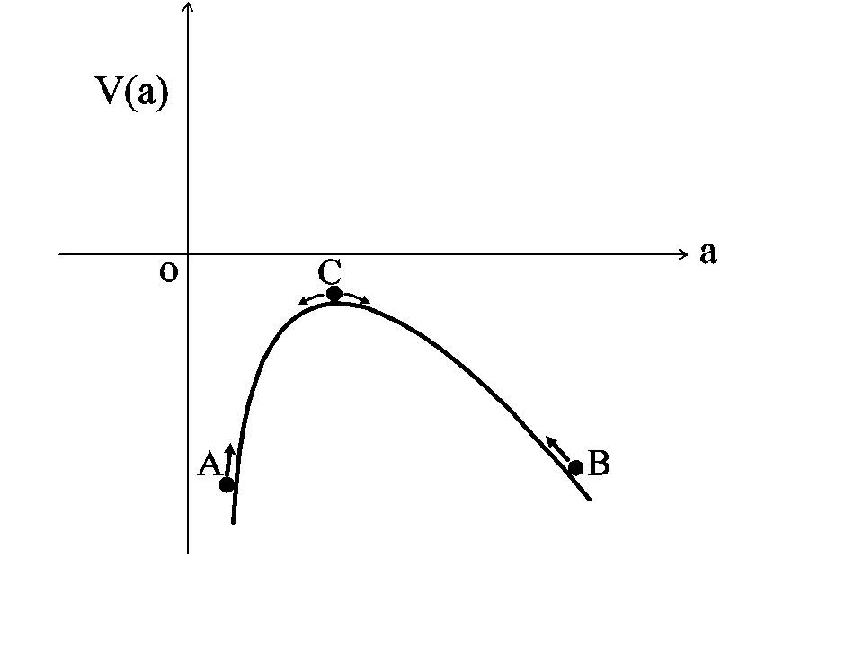
Figure 1: Figure displays the potential V (a) versus the scale factor $a$ . The initial positions (A) and (B) correspond to motion of system beginning from a = 0 and $a=\infty$. For $K<0$ and $\Lambda<\Lambda_{c}$, we have oscillating and bouncing solutions depending whether the motion commences from configuration (A) with $a=0$ or from configuration (B) with $a=\infty$. Einstein static solution($\ddot{a}=0,\dot{a}=0$) corresponds to the maximum of the potential. The case of $\Lambda>\Lambda_{c}$ is similar to $K=0,-1$ such that the kinetic energy is always sufficient to overcome the barrier.

The potential $V(a)$ is concave down and has a maximum where the kinetic energy is minimum (see, Fig.1),

$$\left(\frac{\dot{a}^{2}}{2}\right)_{|_{min}}=\frac{1}{2}\left(C^{2/3}\Lambda^{1/3}-K\right)$$ (10)

where $C=4\pi G\rho^{0}a_{0}^{3}$. If we imagine that motion in Fig.1 commences on the left of the hump, the kinetic energy is always sufficient to overcome the barrier for $K=0$ and $K=-1$ where as in case of $K=1$, we get a bound on the value of $\Lambda\geq\Lambda_{c}=4\pi\rho^{0}a_{0}^{3}$ to achieve the same. Observations have repeatedly conformed the spatially flat nature of geometry $(K=0)$ SN ; cmb ; wmap which is consistent with the prediction of inflationary scenario and we shall adhere to the same in the following discussion. In this case, starting from position (A), see Fig1, one can always reach (C) and before one reaches the hump, motion decelerates followed by acceleration thereafter. Observations have shown that this transition takes place at late times. In order to appreciate it, let us write (6) in the form,

$$H^{2}=H^{2}_{0}\left[\Omega_{m}\left(\frac{a_{0}}{a}\right)^{3}+\Omega_{\Lambda}\right];~{}\Omega_{m}=\frac{\rho_{m}^{0}}{\rho_{cr}},~{}\Omega_{\Lambda}=\frac{\rho_{\Lambda}}{\rho_{cr}},~{}\rho_{cr}=\frac{3H_{0}^{2}}{8\pi G}$$ (11)

It then straight forward to estimate the numerical value of $a_{0}/a$ for which the kinetic energy,

$$\frac{\dot{a}^{2}}{2}=H_{0}^{2}\left[\Omega_{m}\left(\frac{a_{0}}{a}\right)^{3}+\Omega_{\Lambda}a^{2}\right]$$ (12)

is minimum and that happens when,

$$\left(\frac{a_{0}}{a}\right)|_{min}\equiv 1+z_{tr}=\left(\frac{2\Omega_{\Lambda}}{\Omega_{m}}\right)^{1/3}$$ (13)

where we have introduced redshift $z$ which quantifies the effect of expansion. Using the observed values of dimensionless density parameters, $\Omega_{m}\simeq 0.3$ and $\Omega_{\Lambda}\simeq 0.7$, we find that $z_{tr}\simeq 0.67$ which tells us that transition from deceleration to acceleration, indeed, took place recently.

Let us note that cosmological constant is not the only example of negative pressure fluid, a host of scalar field systems can also mimic a negative pressure fluid. An important comment about negative pressure systems is in order. The introduction of $\Lambda$ does not require an adhoc assumption, the latter is always present in Einstein equations by virtue of Bianchi identities. In fact in four dimensions, the only consistent modification(without invoking the extra degrees of freedom)that the Einstein equations allow in the classical regime is given by, $T_{\mu\nu}\to T_{\mu\nu}-\Lambda g_{\mu\nu}$. Actually, this is the other way around that one should provide justification if one wishes to drop the cosmological constant from Einstein equations; there exists no symmetry at low energies to justify the latter. As for the scalar fields, their introduction is quite adhoc and on the top of every thing, one switches off $\Lambda$ for no known reason. Scalar fields, however, may be of interest if they are inspired by a fundamental theory of high energy physics.

II.1 Age crisis in hot big bang and the need for a repulsive effect

At early epochs, radiation dominates, its energy density is large, as a result, the expansion rate is also large. Consequently, it does not take much time to reach a given expansion rate in the early universe. For instance, Universe was around $10^{5}$ years old at the radiation matter equality which is negligible compared to the age of universe. It is therefore clear that most of the contribution to the age of universe comes from matter dominated era at late stages. In order to appreciate the role of $\Lambda$, let us switch it off in the Friedmann equation. Then for matter dominated Universe ($K=0$), the Friedmann equation (3) readily integrates to,

$$a(t)\propto t^{2/3}\to H=\frac{2}{3t}$$ (14)

and specializing to the present epoch, we have

$$t_{0}=\frac{2}{3}\frac{1}{H_{0}}$$ (15)

Recent observations reveal that

$$H^{-1}_{0}\simeq 1.4\times 10^{9}years\to t_{0}\simeq 9.4\times 10^{9}years$$ (16)

which falls much shorter than the age of some well known objects (around 14 billion years) in the universe Krauss:1995yb ; Turner:1997de ; Krauss . Actually, the factor of $2/3$ in (15) spoils the estimate. Let us argue on physical grounds as how to address the problem. In presence of normal matter, gravity is attractive and it decelerates the motion. If gravity could be ignored, then using the Hubble law, $v=Hr$($v=const$), we could have, $t_{0}=1/H_{0}$ which is what is required. However, we can not ignore gravity, there is around 30 $\%$ of matter present in the universe which causes deceleration of the expansion and reduces the age of universe. The only way out to decrease the influence of the matter is to introduce a repulsive effect necessary to encounter the gravitational attraction of normal matter. Let us stress that this is the only known possibility to improve upon the age of universe in the standard model of Universe. Indeed using the Friedmann equation, we can estimate the time universe has spent starting from the big bang till today or the age of universe $t_{0}$,

$$t_{0}=\frac{1}{H_{0}}\int_{0}^{\infty}{\frac{dz}{(1+z)\sqrt{\Omega_{m}(1+z)^{3}+\Omega_{\Lambda}}}}$$ (17)

where we have used the change of variable, $dt=-dz/H(1+z)$. The age of the universe is then finally given by,

$$t_{0}H_{0}=\frac{2}{3}\frac{1}{\Omega_{\Lambda}^{1/2}}\ln\left(\frac{1+\Omega_{\Lambda}^{1/2}}{\Omega_{m}^{1/2}}\right)$$ (18)

Expression (18) tells us that $t_{0}H_{0}\simeq 1$ for the observed values of density parameters, $\Omega_{\Lambda}\simeq 0.7$ and $\Omega_{m}\simeq 0.3$. Thus the late time inconsistency of hot big bang cries for cosmological constant.
It is really interesting to note that there exists no such problem in Hoyle-Narlikar steady state cosmology Hoyle1 ; Hoyle2 which thanks to the perfect cosmological principal has no beginning and no end. Also, the study state theory imbibes cosmic acceleration and does not suffer from the logical inconsistencies the standard model is plagued with. Unfortunately, the model faces problems related to thermalization of the microwave background radiation. However, the generalized steady state theory dubbed ”Quasi Steady State Cosmology” (QSSC) formulated by Hoyle, Burbidge and Narlikar claims to explain the CMBR as well as derive its present temperature which the big bang cannot dojvnb .

II.2 Theoretical issues associated with cosmological constant

It is clear from the aforesaid that cosmological constant is essentially present in Einstein equations as a free parameter which should be fixed by observations. Sakharov pointed out in 1968 Sakharov:1967pk that quantum fluctuations would correct this bere value. In flat space time, according to Sakharov, a field placed in vacuum would have energy momentum tensor

$$<0|T_{\mu\nu}|0>=-\rho_{v}\eta_{\mu\nu}$$ (19)

uniquely fixed by relativistic invariance. $\rho_{v}$ dubbed vacuum energy density is constant by virtue of conservation of energy momentum tensor. Keeping in mind the perfect fluid form of the energy momentum tensor, we have, $p_{v}=-\rho_{v}$ which is the expression of relativistic invariance. The curved space time generalization is given by

$$<0|T_{\mu\nu}|0>=-\rho_{v}g_{\mu\nu}$$ (20)

which should be added to the bare value of cosmological constant present in Einstein equations,

$$R_{\mu\nu}-\frac{1}{2}Rg_{\mu\nu}+g_{\mu\nu}\Lambda_{b}=T_{\mu\nu}^{m}+<0|T_{\mu\nu}|0>$$ (21)

A free scalar field is an infinite collection of non interacting harmonic oscillators whose zero point energy is the vacuum energy of the scalar field,

$$\rho_{v}=\frac{1}{2}\int_{0}^{\infty}{\frac{4\pi k^{2}dk}{(2\pi)^{2}}\sqrt{k^{2}+m^{2}}}$$ (22)

and incorporating spin does not change the estimate. Expression (22) is formally divergent and requires a cut off. One normally cuts it off at Planck’s scale as an expression of our ignorance and concludes that $\rho_{v}\sim M^{4}_{p}$. Using then the Friedmann equation expressed through dimensionless density parameters,

$$\Omega^{eff}_{\Lambda}+\Omega_{m}=1$$ (23)

one finds, $\rho_{\Lambda}^{eff}\lesssim\rho_{cr}\sim 10^{-120}M^{2}_{p}$ which is the source of a grave problem. And since,

$$\rho^{eff}_{\Lambda}=\rho^{b}_{\Lambda}+\rho_{v},$$ (24)

it follows that $\rho^{b}_{\Lambda}$ should cancel $\rho_{v}$ to a fantastic accuracy, typically, at the level of one part in $10^{-120}$. The supernovae Ia observation in 1998 revealed that effective vacuum energy is not only small, it is of the order of matter density today.

The cosmological constant problem is often formulated as,
$\bullet$ Old problem(before 1998): Why effective vacuum energy is so small today?Wg ,
$\bullet$ New problem(after 1998): Why we happen to live in special times when dark energy density is of the order of matter density? a la coincidence problem Steinhardt:1999nw .

We should point out a flaw in the above argumentsahmad . We should bear in mind that the cut off used on 3-momentum violates Lorentz invariance and might lead to wrong results. In what follows, we shall explicitly demonstrate it.

Lorentz invariance signifies a particular relation between vacuum energy $\rho_{v}$ and vacuum pressure $p_{v}$, namely, $\rho_{v}=-p_{v}$. Similar to the vacuum energy, the vacuum pressure is formally divergent and also requires a cut off. Introducing a cut off $M$ in the divergent integrals and expressing $\rho_{v}$ and $p_{v}$, we have,

$$\rho_{v}=\frac{1}{2(2\pi)^{3}}\int_{0}^{\infty}{d^{3}{\bf k}~{}\omega(k)}$$ (25)

$$p_{v}=\frac{1}{6(2\pi)^{3}}\int_{0}^{\infty}{d^{3}{\bf k}\frac{k^{2}}{w(k)}};~{}~{}w(k)=\sqrt{k^{2}+m^{2}}$$ (26)

which allows us to compute these quantities,

$$\rho_{v}=\frac{1}{4\pi^{2}}\int_{0}^{M}{dkk^{2}\sqrt{k^{2}+m^{2}}}=\frac{M^{4}}{16\pi^{2}}\left[\sqrt{1+\frac{m^{2}}{M^{2}}}\left(1+\frac{m^{2}}{2M^{2}}\right)-\frac{1}{2}\frac{m^{4}}{M^{4}}\ln\left(\frac{M}{m}+\frac{M}{m}\sqrt{1+\frac{m^{2}}{M^{2}}}\right)\right]$$ (27)

$$p_{v}=\frac{1}{3}\frac{1}{4\pi^{2}}\int_{0}^{M}{dk\frac{k^{4}}{\sqrt{k^{2}+m^{2}}}}=\frac{1}{3}\frac{M^{4}}{16\pi^{2}}\left[\sqrt{1+\frac{m^{2}}{M^{2}}}\left(1-\frac{3M^{2}}{2M^{2}}\right)+\frac{3m^{4}}{2M^{4}}\ln\left(\frac{M}{m}+\frac{M}{m}\sqrt{1+\frac{m^{2}}{M^{2}}}\right)\right]$$ (28)

In the expressions quoted above, $m$ is the mass of the scalar field placed in vacuum. Invoking spin contribution does not alter the estimates. Hence $\rho_{v}$ and $p_{v}$ given by (27) $\&$ (28) are valid estimates for any field placed in vacuum. Secondly, as mentioned before, for Lorentz invariance to hold we should have $\rho_{v}=-p_{v}$ which is clearly violated by the first terms in (27) and (28 ). It should be noted that this is the first term in these expressions which gives contribution proportional to $M^{4}$. As for the second terms with logarithmic dependence on the cut off, they are in accordance with Lorentz invariance.
It is therefore clear that we should employ a regularization scheme which respects Lorentz invariance. For instance, dimensional regularization is suitable to the problem. Let us first transform the integral from four to $d$ dimension,

$$\rho_{v}=\frac{\mu^{4-d}}{2(2\pi)^{(d-1)}}\int_{0}^{\infty}{dkk^{d-2}d^{d-2}\Omega~{}\omega(k)}$$ (29)

where the scale $\mu$ is introduced to take care of the units in $d$ dimensional case and $\Omega$ is the solid angle . This integral can expressed through gamma function,

$$\rho_{v}=\frac{\mu^{4}}{2(4\pi)^{(d-1)/2}}\frac{\Gamma(-d/2)}{\Gamma(-1/2)}\left(\frac{m}{\mu}\right)^{d}$$ (30)

Finally, we should return to four dimensions by letting $d=4-\epsilon$ and expanding the result in $\epsilon$ to the leading order,

$$\rho_{v}=-\frac{m^{4}}{64\pi^{2}}\left(\frac{2}{\epsilon}+\frac{3}{2}-\gamma-\ln\left(\frac{m^{2}}{4\pi\mu^{2}}\right)\right)+..$$ (31)

which diverges as $\epsilon\to 0$. We have successfully isolated the divergence without violating Lorentz invariance. We then subtract out infinity to obtain the final result,

$$\rho_{v}\simeq\frac{m^{4}}{64\pi^{2}}\ln\left(\frac{m^{2}}{\mu^{2}}\right)$$ (32)

In order to estimate the vacuum energy, we should imagine all the fields placed in vacuum and sum up their contributions. To be pragmatic, we use the following data from standard model of particle physics to estimate $\rho_{v}$

$$m_{t}\simeq 171GeV;m_{H}\simeq 125GeV;~{}~{}m_{z,w}\simeq 90GeV,...$$ (33)

Clearly the stage is set by the heaviest scale in the problem, the mass of the top quark. As for the scale $\mu$, it is always estimated by the physical conditions. In the problem under consideration, the energy scale, $\mu$, is set by the critical energy density and the energy density characterized by the wavelength of light received from supernovae,

$$\mu\sim\sqrt{H_{0}E_{\gamma}},H_{0}\sim 10^{-41}GeV;~{}\lambda\sim 500nm$$ (34)

$$\mu\sim\sqrt{H_{0}E_{\gamma}}\to\rho_{v}\simeq 10^{8}GeV^{4}$$ (35)

which shows that effective vacuum energy density is down by sixty four orders of magnitude compared to the one obtained using the Lorentz violating regularization. And this considerably reduces the fine tuning at the level of standard model,

$$\rho^{eff}_{\Lambda}\simeq 10^{-56}M_{p}^{4}$$ (36)

Thus fine tuning is one part in $10^{-56}$, rather than one part in $10^{-120}$ as often quoted, provided we believe that there is no physics beyond standard model. But we know that there is at least one scale beyond, associated with gravity, namely, the Planck scale which would take us back to original fine tuning problem if the Planck scale is fundamental. However, if it is a derived scale similar to the one in Randall-Sundrum scenario, the fine tuning could considerable reduce. We thus conclude that the cosmological constant problem a la fine tuning could not be as severe as it is posed; it is often over emphasized. Of course the problem still remains to be grave.
The coincidence problem or why dark energy density is of the order of matter density today? is yet more over emphasized. We know that universe went through a crucial transition between $z=1$ to $z=0$. Let us ask how much time universe has spent beginning from a given redshift $z$ to the present epoch. Using Eq.(17), it is straight forward to write down the expression for $t_{z}$,

$$t_{z}=\frac{1}{H_{0}}\int_{0}^{z}{\frac{dz^{\prime}}{(1+z^{\prime})\sqrt{\Omega_{m}(1+z^{\prime})^{3}+\Omega_{\Lambda}}}}$$ (37)

where the dimensionless density parameters are specialized to the present epoch as before.

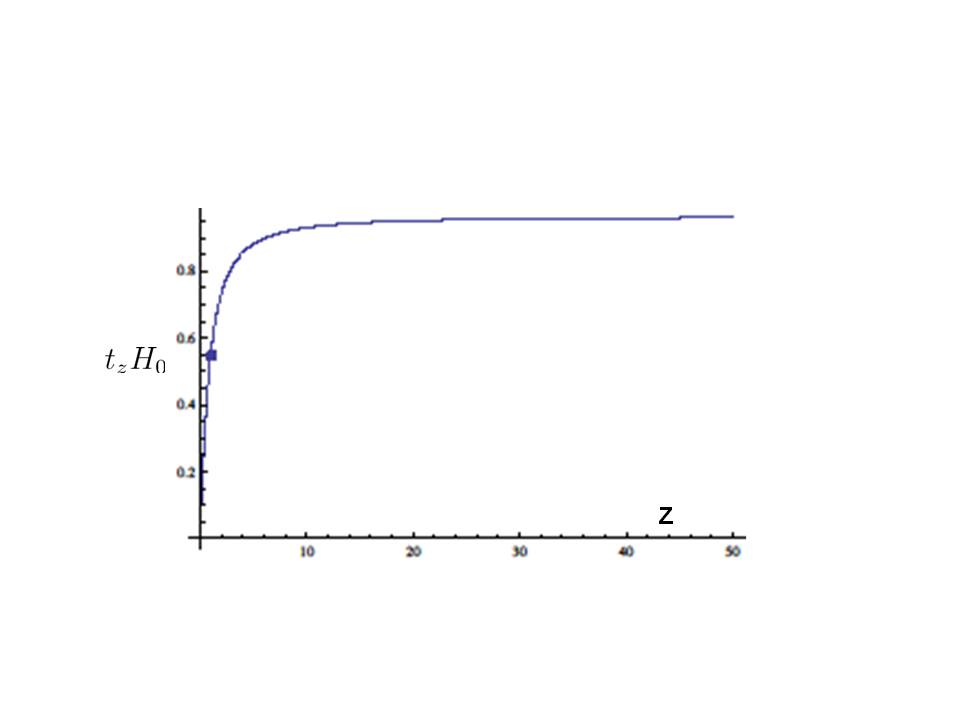
Figure 2: Figure shows the time universe has spent beginning from particular value of redshift to the present epoch. The black dot on the curve corresponds to time universe has spent from $z=1$ to $z=0$ which is more than half of the age of universe. It is clear from the figure that the curve fast saturates as $z$ increases and that most of the contribution to the age comes from the matter dominated era, (z=4,0)

It is clear from the Fig.2 that most of the contribution to age comes from late stage of evolution. Universe spent more than half of its age in the interval between $z=1$ and the present epoch, $z=0$ and during this period matter density and dark energy density remained roughly within the same order of magnitude. Thus they have been within one order of magnitude for ages thereby telling us that there is hardly any coincidence problemcarlo .

III Quintessence and its difficulties

Slowly rolling scalar fields, broadly referred to as ${\it quintessence}$ quint , were introduced with a hope to alleviate the fine tuning problem. Scalar field models applied to cosmological dynamics can be classified into two types $-$ trackers Steinhardt:1999nw and thawing Caldwell:2005tm models. Trackers are interesting for the reason that dynamics in this case is independent of initial conditions where as the thawing models involve dependency on initial conditions with the same level of fine tuning at par with cosmological constant.

Let us briefly consider the cosmological dynamics of a scalar field which can be treated as a perfect fluid with energy density $\rho_{\phi}$ and pressure $p_{\phi}$ given by(see Ref.review2 for details),

$$\rho_{\phi}=\frac{\dot{\phi}^{2}}{2}+V(\phi)~{}~{};p_{\phi}=\frac{\dot{\phi}^{2}}{2}-V(\phi);~{}~{}\omega_{\phi}\equiv\frac{p_{\phi}}{\rho_{\phi}}$$ (38)

For slowly evolving field, $\omega_{\phi}\simeq-1$ whereas $\omega_{\phi}\simeq 1$ if field rolls fast which happens for a steep potential. The equation of motion for the standard scalar field $\phi$ in FRW cosmology is,

$$\ddot{\phi}+3H\dot{\phi}+V^{\prime}(\phi)=0$$ (39)

where the second term is due to Hubble damping. From (39), we infer that

$$\rho_{\phi}=\rho_{\phi}^{0}\exp{\left(-\int{3(1+\omega_{\phi})\frac{da}{a}}\right)}$$ (40)

which tells us that $\rho_{\phi}\sim 1/a^{6}$ in case the field is rolling along a steep potential. Let us consider an exponential potential which has served as a laboratory for the understanding of cosmological dynamics Copeland:1997et ; Nunes:2000yc ,

$$V(\phi)=V_{0}e^{-\lambda\phi/M_{p}}$$ (41)

Figure 3: Figure shows evolution of $\rho_{\phi}$ and background energy density versus the scale factor on the logarithmic scale. As the field emerges from locking regime, it tracks the background. At late times, it begins to approach $\rho_{b}$ and finally overtakes to become dominant giving rise to late time acceleration. Once the present epoch is set by suitably choosing the model parameters, evolution is independent of initial conditions.

The parameter $\epsilon=M^{2}_{p}(V^{\prime}/V)^{2}/2$ then sets a condition for slow roll, namely, $\lambda<\sqrt{2}$. The slow roll parameters do not play the same role here as they do in case of inflation due to the presence of matter but still can guide us for the broad picture. A suitable choice of $\lambda$ can give rise to viable late time cosmic evolution. The de Sitter solution is an attractor of the system. There is one more remarkable attractor in the system that exists in presence of background (matter/radiation) dubbed scaling solution which exists for a steep potential with $\lambda\geq\sqrt{3}$. Let us consider the case when field energy density is initially larger than the background energy density, $\rho_{b}=\rho_{r}/\rho_{m}$, see Fig.3. Since the potential is steep, $\rho_{\phi}$ redshifts faster than $\rho_{b}$ and the field overshoots the background such that $\rho_{\phi}<<\rho_{b}$. In that case, the Hubble damping in the field evolution equation is enormous and consequently, the field freezes on its potential such that $\rho_{\phi}=const$. Meanwhile the background energy density redshifts with the expansion and the field waits till the moment its energy density becomes comparable to that of the background, thereafter the evolution can proceed in two ways depending upon the nature of the potential: (1) : In case of (steep) exponential potential, field would track the background; in matter dominated era, field would mimic matter $(\omega_{\phi}=\omega_{m})$ for ever. This is a very useful attractor dubbed scaling solution though not suitable to late time acceleration. In this case, we shall need a feature in the potential that would give rise to the exit from scaling solution at late times, see Fig.3. (2) In this case, field begins to evolve and overtakes the background without following it which happens if the field rolls slow at late times. This happens in case of a potential which is steep but not exponential at early epochs and shallow at late times. For such potentials, evolution crucially depends upon the initial conditions. In this case, though we can have suitable late time evolution but the model is faced with the same fine tuning problem as the one based upon cosmological constant; models with shallow potential throughout are faced with the same problem. Models of this class are termed as thawing models, see Fig.4. Let us note that the requirement to obtain a tracker solution is very specific and only a small number of field potentials in case of a standard scalar field can give rise to tracker solutions. As for the tachyonsamio or phantomphantom1 ; phantom2 fields, there exists no realistic tracker (that could tracker the standard matter); irrespective of their potential they belong to the class of thawing models.

Figure 4: The figure shows the evolution of field energy density along with the background matter density $\rho_{b}$ on log scale. Initially, field rolls along steep part of the potential, redshifts faster than $\rho_{b}$, overshoots it and freezes due to large Hubble damping. In this case, after the exit from locking regime, field begins to roll slowly and overtakes the background and can account for late time cosmic acceleration. In this case changing initial conditions would disturb present day physics which can be restored by resetting the model parameters. In this case, evolution depends upon initial conditions. The level of fine tuning is at par with cosmological constant

What is a desirable quintessence field for thermal history and late time cosmic evolution? Actually, we should look for a model with steep exponential potential throughout most of the history of universe and a shallow one at late times. In that case, the field would assume the scaling behavior after the exit from locking regime and only at late times it would leave it to become dominant and give rise to late time cosmic evolution a la tracker solution, see Fig.3 Steinhardt:1999nw . In this case, evolution is independent of initial conditions and the fine tuning associated with $\Lambda$ may be alleviated. It is possible to realize tracker solutions in several ways. However, they are obtained most naturally in models with inverse power law potentials ($V\sim 1/\phi^{n}$) which approximate the exponential potential for large values of the exponent $n$ and for which the slope is variable$-$ large at early epochs and small at late times which is precisely the behavior we are looking for. It is little discouraging that tracker models are less favored observationally compared to thawing models.

The slowly rolling scalar field models irrespective of their types are generally faced with another grave problem which surfaces when we allow the scalar field interaction with matter, $g\phi\bar{\psi}\psi$. In order to appreciate the problem, let us estimate the mass of scalar field employing any of the slow roll conditions,

$$\epsilon=\frac{M^{2}_{p}}{2}\left(\frac{V^{\prime}}{V}\right)^{2}<<1;~{}\eta=M^{2}_{p}\frac{V^{\prime\prime}}{V}<<1$$ (42)

and since the mass of the field should be of the order of $H_{0}$ to be relevant to late time cosmic acceleration, we find by making use of the second slow roll parameter $\eta$,

$$m^{2}\simeq V^{\prime\prime}\simeq\frac{V}{M^{2}_{p}}\simeq\frac{H^{2}_{0}M^{2}_{p}}{M^{2}_{p}}\simeq\left(10^{-33}eV\right)^{2}$$ (43)

An important remark related to late time field dynamics is in order. In case, $m>>H_{0}$, the field would be rolling very fast at the present epoch and hence of no relevance to late time cosmology. On the other hand, if $m<<H_{0}$, the field would not be distinguished from cosmological constant. Therefore, the quintessence mass should be precisely of the order of $H_{0}$.
The tiny mass of the field creates problem as one loop correction shifts the mass of the field by a huge amount $m^{2}\to m^{2}+gM^{2}$(M is cut off) unless we tune the coupling $g$ appropriately. Since $m^{2}\sim H^{2}_{0}$, the required fine tuning brings us back to cosmological constant. Since there are no known symmetries at low energies to control the radiative corrections, the purpose of introducing dynamical dark energy this way stands defeated. Let us mention an attempt to construct a string inspired axionic quintessence for which the radiative corrections might be under controltrivedi . However, the scenario belongs to the class of thawing models and thereby faced with the same level of fine tuning as cosmological constant.

Before we get to the next topic, we would like to comment on the stability of fundamental scalar against radiative corrections. One might think that the large correction to mass is the artifact of the regularization as dimensional scheme of regularization always involves logarithmic dependence on the cut off.In order to clarify the issue, let us accurately compute the one loop correction to mass of the fundamental scalar,

$$(\delta m^{2})_{1~{}loop}\sim\int{\frac{d^{4}k}{k^{2}+m_{s}^{2}}}\sim M^{2}+m_{s}^{2}\ln M^{2}/m_{s}^{2}$$ (44)

where $m_{s}$ is the mass of field circulating in the loop and $M$ is the cut off on four momentum introduced to compute the divergent integral. It should be noticed that unlike the calculation of vacuum energy, the cut off used here preserves Lorentz invariance. Secondly, one often quotes the first term of (44) as correction to mass which is quadratic divergent (as we did above) when cut off is removed. Let us compute the same using dimensional regularization,

$$(\delta m^{2})_{1~{}loop}\sim\int{\frac{d^{4}k}{k^{2}+m_{s}^{2}}}\sim\frac{1}{\epsilon}+m_{s}^{2}\ln\frac{m_{s}^{2}}{\mu^{2}}$$ (46)

We notice that the first terms in both the expressions (44) $\&$ (46) are divergent and need to be subtracted; the remaining logarithmic corrections are essentially same whether we impose simple cut off on four momenta in the divergent integral or we employ the dimensional regularization. We should emphasize that it is the property of the fundamental scalar that the radiative correction to its mass is proportional to the mass of the field it interacts with. The dominant contribution comes from the heaviest mass scale in the theory to which the one loop correction is proportional to. In case there is such a mass scale in the theory, it would destabilize the system as there is no symmetry to protect it at low energies. This is a generic problem inherent to theories that include a fundamental scalar and it has nothing to do with the regularization scheme we use. Indeed, the same does not happen in electrodynamics where the one loop correction to mass of electron is given by,

$$(\delta m_{e}^{2})_{1~{}loop}\sim e^{2}m_{e}^{2}\ln M^{2}/m_{e}^{2}$$ (47)

which is remarkable in a sense that atomic physics can rely on the interaction of electrons and photons and can safely ignore heavier fermions; their contribution is suppressed by inverse powers of the corresponding heavier mass scales which is radically different from what happens in theory with a fundamental scalar.

III.1 Cosmological constant, scalar field and t’ Hooft criteria of naturalness

In a healthy field theoretic set up, the higher mass scales are expected to decouple from low energy physics. According to t’Hooft, a parameter in the field theory is termed natural if by switching it off in Lagrangian at the classical level enhances symmetry of theory which is also respected at the quantum level. Let us immediately note that cosmological constant is not a natural parameter of Einstein theory. Indeed, in absence of matter, if we ignore $\Lambda_{b}$, Eintein equations(21) admit Minkowsky space time as solution. In this case, the underlying symmetry group, namely, the Poincare group has 10 generators similar to the case of de Sitter space time that one obtains as solution after invoking cosmological constant in Einstein equations. We therefore conclude that cosmological constant is not a natural parameter of Einstein theory. It is also clear from the above discussion that any field theory that contains a fundamental scalar suffers from the problem of naturalness see Ref.smyr for details. In these theories a protection mechanism should be in place. The recent discovery of Higgs boson of mass around 125 GeV cries for supersymmetry essential for the consistency of the framework. Clearly, both the cosmological constant and scalar field are faced with problem of similar nature.

Let us also emphasize that in field theory formulated in flat space time, vacuum energy can safely be ignored by choosing normal ordering. It is legitimate as there is no known laboratory experiment to measure the absolute value of energy; we normally measure the difference such that the vacuum energy gets canceled in the process. Can’t we then play the following trick to address the cosmological constant problem? Indeed, the FRW metric, is conformally equivalent to Minkowsky space time. By a suitable conformal transformation on Einstein-Hilbert action with cosmological constant, we can transform to flat space time. However, in this case, we are left with scalar field non-minimally coupled to matter. Taking into account the fact that particle masses in the Einstein frame become field dependent, one can demonstrate that the scalar field in flat space time imbibes full information of FRW dynamics. Have we then done away with cosmological constant problem? Unfortunately, scalar field as we pointed out is plagued with the problem of naturalness thereby one problem translates into another equivalent one.

IV Large scale modification of gravity and its relevance to late time cosmic acceleration

As mentioned before, the modified theories of gravity at large scales are essentially represented by Einstein Gravity(GR) along with the extra degrees of freedom. For instance, in $f(R)$ theories no ; Sotiriou:2008rp ; DeFelice:2010aj , we have one scalar degree of freedom $\varphi$ dubbed scalaron which is mixed with the curvature in the Jordan frame. We can diagonalize the Lagrangian by performing a conformal transformation on $f(R)$ action reducing the theory in Einstein frame to GR plus a scalar field with a potential uniquely determined through $R$ and the first derivative of f(R) with respect to R. Consistency demands that $f^{\prime}>0$ (absence of ghost) and$f^{\prime\prime}>0$(absence of tachyonic mode or Dolgov- Kawasaki instability). In Einstein frame, degrees of freedom become diagonalized but $\varphi$ gets directly coupled to matter and the coupling is typically of the order of one. We emphasize that both the frames are not only mathematically equivalent but also describe same physics: the relationship between physical observables is same in both the frames. The extra degree of freedom $\varphi$ should give rise to rise to late time cosmic acceleration thereby telling us that its mass $m_{\varphi}\sim H^{2}_{0}$. However, such a light field directly coupled to matter would grossly violate the local physics where GR is in excellent agreement with observations . For instance, solar physics would be safe if $m_{\varphi}>10^{-27}$. It is an irony that large scale modification interferes with local physics which is related to the fact that GR describes local physics to a very high accuracy. Thus, if $f(R)$ to be relevant to late time cosmic acceleration, the scalaron should appear light at large scales and heavy locally in high density regime a la a chameleon field Khoury:2003rn ; Khoury:2003aq . In what follows, we shall present basic features of large scale modification of gravity.

IV.1 Modified theories of gravity

An important class of modified theories can be described by generalized scalar tensor theories. Let us for simplicity consider the following action in Einstein frame,

$$\mathcal{S}=\int{\sqrt{-g}d^{4}x\Big{[}\frac{M^{2}_{p}}{2}R-\frac{1}{2}(\partial_{\mu}\phi)^{2}-V(\phi)\Big{]}}-\int{\sqrt{-g}d^{4}x\mathcal{L}_{m}(\psi,A^{2}(\phi)g_{\mu\nu})}$$ (48)

where $\psi$ are the matter fields and $A(\phi)$ is the conformal coupling which relates Einstein metric $g_{\mu\nu}$ with the Jordan metric as,

$$\tilde{g}_{\mu\nu}\equiv A^{2}g_{\mu\nu}$$ (49)

and appears in the matter Lagrangian. We can generalize the scalar field Lagrangian in (48) by including non linear higher derivative terms dubbed galileons Luty:2003vm ; Nicolis:2004qq ; Nicolis:2008in ; Deffayet:2009wt , Deffayet:2009mn ; Trodden:2011xh ; Deffayet:2011gz ; deRham:2010eu ; Goon:2011qf ; DeFelice:2010nf ; Shirai:2012iw or generalized galieonsa la Hordenski field Horndeski:1974wa ; Deffayet:2013lga . We shall provide outline of galileon field dynamics in the discussion to follow. Going ahead, we wish to point out that these fields are central to Vainshtein screening which in turn are at the heart of massive gravity Fierz:1939ix ; ArkaniHamed:2002sp ; deRham:2010ik ; deRham:2010kj ; Hassan:2011hr ; deRham:2011rn ; Hassan:2011zd ; deRham:2010tw ; Creminelli:2005qk (for review, see Ref.Hinterbichler:2011tt ). In the discussion to follow, we shall first consider scalar field with potential suitable to implement chameleon mechanism and then turn to massless field and its screening using kinetic suppression.

In case of a massive field, it is instructive to write down the equation of motion for the field in presence of the conformal coupling by varying the action (48),

$$\Box\phi=-A^{\prime}(\phi)T+\frac{dV}{d\phi}=-\frac{\alpha}{M_{p}}T+\frac{dV}{d\phi};~{}~{}\alpha\equiv M_{p}\frac{d\ln A(\phi)}{d\phi}$$ (50)

where $\alpha$ is coupling constant and for simplicity, we assume that $A(\phi)\simeq 1+\alpha\phi/M_{p}(\phi/M_{p}<<1)$. Let us note that $f(R)$ theories correspond to $\alpha=1/\sqrt{6}$. It is important to understand the physical meaning of $\phi$ which becomes clear by considering the Newtonian limit in presence of the conformal coupling. In this case, the geodesics equation is given by,

$$\frac{d^{2}x^{\mu}}{d\tau}+\Gamma^{\mu}_{\alpha\beta}\frac{dx^{\alpha}}{d\tau}\frac{dx^{\beta}}{d\tau}+\frac{\alpha}{M_{p}}\partial^{\mu}\phi\simeq 0$$ (51)

where the last term in the above equation is sourced by the conformal coupling. The second term in (V.3) in Newtonian limit yields the gradient of Newtonian potential with minus sign supplemented by the third term due to conformal coupling,

$$\Phi_{tot}=\Phi_{N}+\frac{\alpha}{M_{p}}\phi$$ (52)

We should once again remind ourselves that $\alpha$ is of the order of one in which case the contribution of the additional term may become comparable to $\Phi_{N}$. In such a scenario, the local physics would be disturbed as the latter is described by GR with a fantastic accuracy. We, therefore, need to locally screen out the effects of the extra force (fifth force) to a great accuracy which is implemented by the chameleon mechanism for a massive field. Before we move ahead it might be instructive to transform the action (48) back to Jordan frame,

$$\int{d^{4}x\sqrt{-g}\Big{[}\frac{M^{2}_{p}}{2}\Phi\tilde{R}-\frac{M^{2}_{p}}{2}\frac{\omega(\Phi)}{\Phi}\tilde{g}^{\alpha\beta}\partial_{\alpha}\Phi\partial_{\beta}\Phi-\Phi^{2}V(\Phi)\Big{]}}+\int{d^{4}x\sqrt{-\tilde{g}}\mathcal{L}_{m}(\psi,\tilde{g}_{\mu\nu}})$$ (53)

where $\Phi=A^{-2}(\phi)$ and $\omega(\phi)$ is given by,

$$\omega(\phi)=\frac{1}{2}\left[\frac{1}{2M^{2}_{p}\left(\frac{A^{\prime}}{A}\right)^{2}}-3\right]\to\frac{1}{\alpha^{2}}=2\omega(\phi)+6.$$ (54)

Here “prime” $(\ \ ^{\prime}\ )$ denotes derivative with respect to the field. Let us comment on relation of Brans-Dicke parameter and the coupling constant $\alpha$. It follows from (54) that $\alpha=1/\sqrt{6}$ for $\omega=0$ which corresponds to $f(R)$ . The coupling constant $\alpha$ as we repeatedly mentioned is typically of the order of one whereas local gravity constrains demand that $\omega\gtrsim 4\times 10^{4}$ correspondingly $\alpha$ is vanishingly small. The latter describes the trivial regime of scalar tensor theories and one is dealing in that case with a coupled quintessence with negligibly small coupling. If accelerated expansion takes place in this case, it is definitely due to flatness of the potential. In such cases one does not need chameleon mechanism and corresponding scalar theories are of little interest. Let us also note that at the onset it appears from (53), that $G_{eff}=A(\phi)G$. However, what one measures in Cavendish experiment is different and can be inferred, for instance, from weak field limit EspositoFarese:2000ij ,

$$G_{eff}=GA(\phi)\left(1+2\alpha^{2}\right)$$ (55)

where the expression in parenthesis is due to the exchange of the scalaron.

It is clear from the aforesaid that chameleon is essential for generic modified theories. In what follows we outline the underlying concept of chameleon screening.

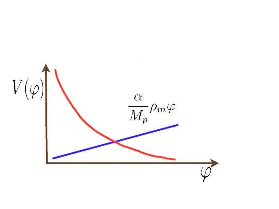
Figure 5: Effective potential for a chameleon field. $V(\phi)$ is generically a run away potential without a minimum. The effect of direct coupling with matter modifies the potential such that the effective potential acquires minimum. Higher is the density of environment, closer would be the minimum to the origin. The potential is a monotonically decreasing function(we might imagine, ($V\sim 1/\phi^{n}$) such that its second derivative $V^{\prime\prime}(\phi)$ is also monotonically decreasing and positive.

IV.2 Chameleon theories: basic idea

In order to set the basic notions of chameleon screening, let us first for simplicity consider a massive scalar field non-minimally coupled to matter Amendola:1999er ,

$$\mathcal{L}=-\frac{1}{2}\partial_{\mu}\varphi\partial^{\mu}\varphi-\frac{1}{2}m^{2}\varphi^{2}+\frac{\alpha}{M_{p}}\varphi T$$ (56)

which on varying with respect to $\varphi$ gives the following equation of motion,

$$(\Box+m^{2})\varphi=-\frac{\alpha}{M_{p}}T$$ (57)

In this case, for a given static point source of mass $M$, $r=0,~{}~{}T=-M\delta^{3}(r)$, the potential sourced by the field is given by,

$$\frac{\alpha}{M_{P}}\varphi=-{2\alpha^{2}GM}\frac{e^{-mr}}{r}$$ (58)

which is the extra contribution to the gravitational potential of the point source due to scalaron. The total potential is then given by,

$$\Phi_{tot}=-\frac{GM}{r}\left(1+2\alpha^{2}e^{-mr}\right)$$ (59)

As mentioned before, $\alpha$ is typically of the order of one. Hence the extra force mediated by the exchange of scalaron between two point masses is of the order of the gravitational force for light mass $mr<<1$, relevant to late time cosmic acceleration. The latter is equivalent to $G\to G_{eff}=G(1+2\alpha^{2})$ which is clearly in conflict with local physics. The consistency at the level of solar system demands that $mr_{AU}<<1$ or $m>>10^{-27}GeV$. It is therefore clear that the mass of scalaron should be environment dependent $m(\rho)$ $-$ light in low density regime(at large scales) and heavy in high density regime locally. We shall briefly demonstrate in the discussion to follow how the chameleon field generated by an extended massive source may get effectively decoupled from the source leaving local physics intact.

IV.3 Chameleon at work

Let us briefly examine how the chameleon mechanism operates Khoury:2003rn ; Khoury:2003aq . The aforesaid discussion makes it clear that we should choose a suitable scalar field potential to achieve the goal. The inverse power law potentials are generic, they become shallow at late time and might give rise to late time acceleration. The effective potential in presence of the coupling is given by,

$$V_{eff}=V(\varphi)+\frac{\alpha}{M_{p}}\rho_{m}\varphi$$ (60)

It is clear from Fig. 5 that $V_{eff}$ has a minimum which is closer to the origin higher is the density of the environment. Since $V^{\prime\prime}(\phi)$ is positive and monotonously decreasing for the generic cases, the mass of the field around the minimum is larger higher is the matter density of the environment and vice versa what was sought for .
We next need to compute the field profile for an extended body of mass $\mathcal{M}$. In case of the gravitational potential a la Newton, the answer is simple: the point particle mass in the expression of its gravitational potential gets replace by $\mathcal{M}$. It should be emphasized that such a privilege is restricted to $1/r$ potential only. In any other case and in particular in the case under consideration, the potential of an extended body, apart from its mass would also depend upon its density. The contribution to the field profile coming from the interior gets Yukawa suppressed due to its large mass in high density regime. Contribution, if any, comes from a thin layer under the surface of the body, see Fig.6.

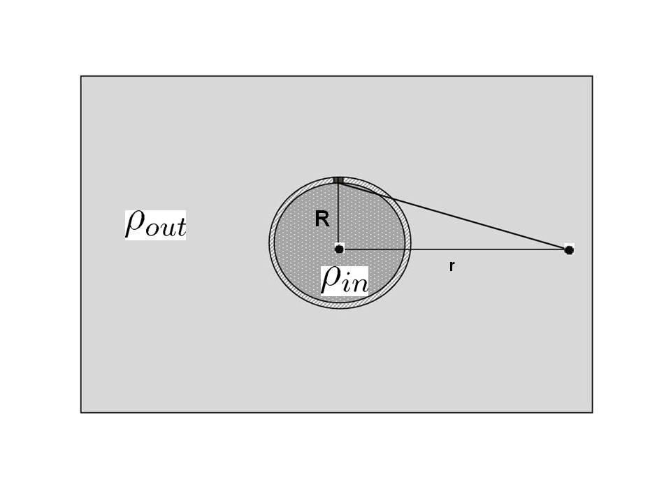
Figure 6: Figure shows a body of mass ${M}$ with a density $\rho_{in}$ embedded in an environment with density $\rho_{out}<<\rho_{in}$. Contribution to the field profile at distance $r$ from the massive body comes from a thin layer under the surface of the massive body due to Yukawa suppression in the interior.

As shown in Refs. Khoury:2003rn ; Khoury:2003aq ,

$$\frac{\alpha}{M_{P}}\varphi=-\frac{GM}{r}\alpha^{2}\epsilon_{thin}$$ (61)

where $\epsilon_{thin}$, the thin shell parameter is given by

$$\epsilon_{thin}\propto\frac{\varphi_{min}^{out}(\rho)-\varphi_{min}^{in}(\rho)}{\Phi_{\mathcal{M}}}$$ (62)

where ${\Phi_{\mathcal{M}}}$ is the Newtonian potential of the extended body. Since, $\varphi_{min}^{in}(\rho)<<\varphi_{min}^{out}(\rho)$ because of the high density inside the body and thus can be dropped. The success of chameleon mechanism then depends upon the fact that the gravitational potential for an extended body, say Sun, is large and $\varphi_{min}^{out}(\rho)$ is small in the solar system. As for the accuracy of GR, the agreement can be reached by suitably choosing model parameters through $\varphi_{min}^{out}(\rho)$. As a result, the effective coupling, $\alpha_{eff}=\alpha\epsilon_{thin}$ in Eq.(61) can be made as small as desired thereby effectively giving rise to decoupling of the field from the source or the screening of the extra force.
At the onset, it looks like that we have succeeded in getting late time cosmic acceleration via the extra degree of freedom $\varphi$, which imbibes large scale modification of gravity, keeping it invisible locally. However, a close scrutiny of chameleon theories reveals that required screening of extra degree(s) leaves no scope of these theories for late time cosmic acceleration. The problem stems from high accuracy of Einstein theory in solar system and laboratory experiments.

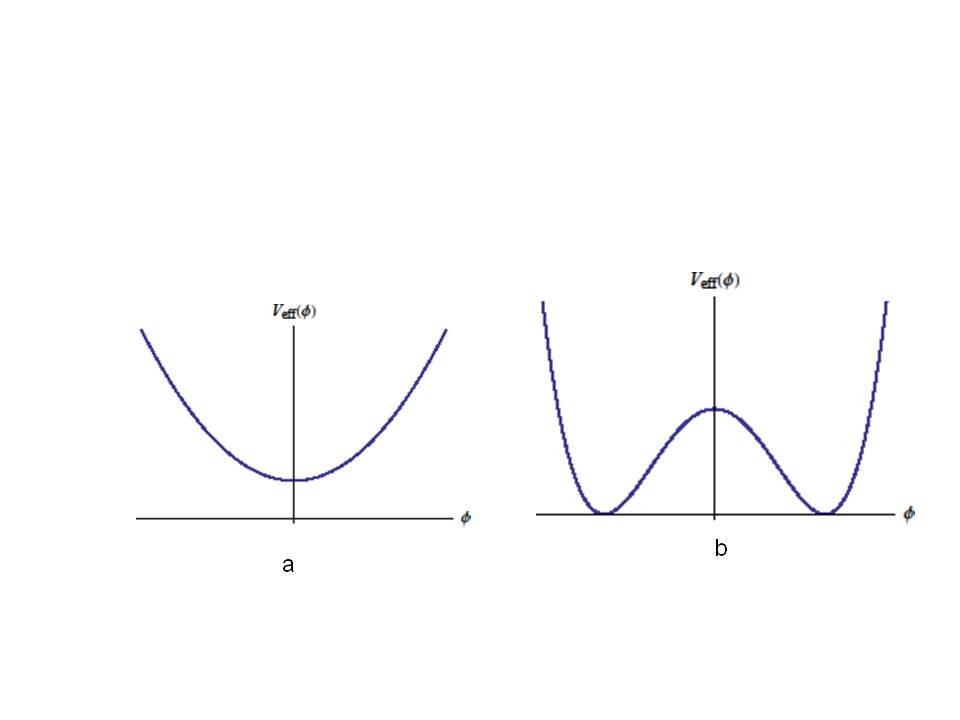
Figure 7: Fig.7(a) displays the symmetron potential in high density regime. In this case the system resides in the symmetric vacuum $\phi=0$. On the other hand, in the low density regime around $\rho=\rho_{cr}$, the symmetric state is no longer a true ground state (Fig.7(b)), the system then makes transition to one of the ground states giving rise to spontaneous symmetry breaking of $Z_{2}$ symmetry of the underlying system

V Spontaneous symmetry breaking in cosmos: A beautiful idea that does not work

As mentioned before, universe has undergone a transition from deceleration to acceleration between $z=0$ and $z=1$. It is tempting to relate the latter to breaking of a hypothetical symmetry which can be realized by invoking a specific conformal coupling Hinterbichler:2010es ; Hinterbichler:2011ca ; Bamba:2012yf . Let us very briefly out line the basic features of the the model dubbed symmetron which is based upon the following Einstein frame action

$$\mathcal{S}=\int d^{4}x\sqrt{-g}\Bigl{[}\frac{M^{2}_{p}}{2}R-\frac{1}{2}\partial_{\mu}\phi\partial^{\mu}\phi-\frac{\mu^{2}}{2}\phi^{2}-\frac{\lambda}{4}\phi^{4}\Bigr{]}+\mathcal{S}_{m}\Bigl{[}A^{2}(\phi)g_{\mu\nu},\Psi_{m}\Bigr{]}$$ (63)

The symmetron potential is invariant under $Z_{2}$ symmetry ($\phi\to-\phi$) and one can preserve this symmetry in the effective potential by making the following choice for $A(\phi)$ Hinterbichler:2010es ; Hinterbichler:2011ca

$$A(\phi)=1+\frac{\phi^{2}}{2M^{2}}~{}(\phi<<M)$$ (64)

where $M$ is a mass scale in the model. The effective potential then takes the following form

$$V_{eff}=\frac{1}{2}\left(\frac{\rho}{M^{2}}-\mu^{2}\right)\phi^{2}+\frac{\lambda}{4}\phi^{4}$$ (65)

The mass of the field now depends upon the density of environment, naively, the field mass is given by, $m^{2}_{eff}={\rho}/{M^{2}}-\mu^{2}$. Thus in high density regime, mass depends upon density linearly, $m^{2}_{eff}\sim\rho/M^{2}>0$. In this case, the system resides in the symmetric vacuum specified by $\phi=0$. The requirement of local gravity constraints puts an upper bound on the mass scale, $M$ and there is no reason for it to be consistent with dark energy. We should note that in case of chameleon, there is more flexibility, the mass depends on density non-linearly. As shown in Ref.Hinterbichler:2010es ; Hinterbichler:2011ca , $M\leq 10^{-4}M_{p}$.
As the density redshifts with expansion and $\rho$ drops below $\mu^{2}/M^{2}$, tachyonic instability builds in the system and the symmetric state $\phi_{0}=0$ is no longer a true minimum. The true minima are then given by(see Fig7)

$$\phi_{0}=\pm\sqrt{\frac{\mu^{2}-\rho/M^{2}}{\lambda}}.$$ (66)

The mass of the symmetron field about the true minimum is given by, $m_{s}=\sqrt{2}\mu$. Universe goes through a crucial transition when late time acceleration sets in around the redshift $z\sim 1$. It is therefore natural to assume that the phase transition or symmetry breaking takes place when $\rho\sim\rho_{cr}$. Hence we conclude that,

$$\rho_{cr}\simeq M^{2}\mu^{2}\to\mu^{2}\simeq\frac{H_{0}^{2}M^{2}_{pl}}{M^{2}}\to m_{s}\simeq\frac{H_{0}M_{p}}{M}$$ (67)

This means that $m_{s}\geq 10^{4}H_{0}$ which is larger than the required quintessence mass by several orders of magnitude. In this case, the field rolls too fast around the present epoch making itself untenable for cosmic acceleration. Invoking the more complicated potential with minimum with the required height does not solve the problem. In this case field would continue oscillating around the minimum for a long time and would not settle in the minimum unless one arranges symmetry breaking very near to $z=0$ by invoking unnatural fine tuning of parameters. There is no doubt that symmetron presents a beautiful idea but, unfortunately, fails to be relevant to late time cosmic acceleration. We believe that it would find a meaningful application in cosmology in some other form.

V.1 Scope of chameleon for late time cosmic acceleration

The large scale modification of gravity effects the gravitational interaction because of the two reasons. (1) The exchange of extra degree(s) of freedom which couples with matter source roughly with the same strength as graviton and whose local influence needs to be screened using a suitable mechanism. (2) The conformal coupling $A(\phi)$ also modifies the strength of gravitational interaction. And to pass the local tests, $A(\phi)$ should be very closely equal to one in high density regime in chameleon supported theories. The transition Universe has undergone during $0<z<1$, is a large scale phenomenon and one might think that the mass screening which is a local effect should not impose severe constraints on how $A(\phi)$ changes during the period acceleration sets in. It turns out that the change the conformal coupling suffers as redshift changes from one to zero is negligibly small. Then the question arises, can such a conformal coupling be relevant to late time acceleration?
It is well known that the de Sitter Universe is conformally equivalent to the Minkowski space-time. Does the conformal transformation changes physics? By ‘physics’, we mean the relationship between physical observables. In the Einstein frame we have the Minkowski space-time where there is a scalar field sourced by the conformal coupling which directly couples to matter. The masses of all material particles are time dependent by virtue of the conformal coupling $A(\phi)$. Consequently, one would see the same relations between physical observables in both the framesmisao . The acceleration dubbed self acceleration is the one which can be removed (caused) by conformal coupling scope . Late time cosmic acceleration which is not related to conformal coupling is caused by the slowly rolling (coupled) quintessence and is not a generic effect of modified theory of gravity. Indeed, this is the case if we adhere to chameleon screening. In what follows we shall describe how it happens. We have the following relation between scale factors in Einstein and Jordan frames,

$$a^{J}(t^{J})=A(\phi)a^{E}(t^{E})\,,\quad dt^{J}=A(\phi)dt^{E}\,,$$ (68)

and as for the conformal time,$dt=a(t)d\eta$, it is same in both the frames . In (68), $a^{J}$( $(a^{E})$) denote scale factor and $t^{J}$( $(t^{E})$) the cosmic time in the Jordan (Einstein) frame.

Let us take the derivatives with respect to the Jordan cosmic time $t^{J}$ of $a^{J}(t_{J})=A(\phi)a^{E}(t^{E})$ left right,

$$\dot{{a}}^{J}(t^{J})=\frac{1}{A}\frac{d}{dt^{E}}\left(Aa^{E}\right)$$ (69)

where derivative of Einstein frame quantities is taken with respect Einstein frame time. Differentiating the last equation again with respect to Jordan time gives,

$$\ddot{a}^{J}(t^{J})=\frac{1}{A}\left(\ddot{a}^{E}+\frac{\ddot{A}}{A}a^{E}-\frac{\dot{A}^{2}}{A^{2}}a^{E}+\frac{\dot{A}}{A}\dot{a}^{E}\right)\,.$$ (70)

By time derivative “dot” $(\ \dot{\ }\ )$ of quantity in the Jordan (Einstein) frame, we mean time derivative with respect to the Jordan (Einstein) time $t^{J}$ ($t^{E}$). Multiplying this equation left right by $a^{J}=Aa^{E}$, we have,

$$\ddot{a}^{J}a^{J}-\ddot{a}^{E}a^{E}=\left(\frac{\ddot{A}}{A}-\frac{\dot{A}^{2}}{A^{2}}\right){(a^{E})}^{2}+\frac{\dot{A}}{A}\dot{a}^{E}a^{E}\,.$$ (71)

The right hand side can be put in compact form by changing the Einstein frame time to the conformal time from $\left(d/dt^{E}\to\left(1/a\right)\left(d/d\eta\right)\right)$.

Indeed, following Ref. scope , we have a relation which relates $\ddot{a}$ in both the frames,

$$\ddot{a}^{J}a^{J}-\ddot{a}^{E}a^{E}=\left(\frac{A^{\prime\prime}}{A}-\frac{A^{\prime 2}}{A^{2}}\right)=\left(\frac{A^{\prime}}{A}\right)^{\prime}\,.$$ (72)

where “prime” $(\ \ ^{\prime}\ )$ denotes the derivative with respect to conformal time in the Einstein frame. Let us note that acceleration in the Einstein frame cannot be caused by conformal coupling,

$$\frac{\ddot{a}}{a}=-\frac{1}{6M_{\mathrm{Pl}}^{2}}\left((\rho_{\phi}+3P_{\phi})+\alpha\rho A(\phi)\right)\,.$$ (73)

Thus in case acceleration takes place in the Einstein frame, it can only be caused by slowly rolling quintessence ($\rho_{\phi}+3P_{\phi}<0$). This implies that acceleration in the Jordan frame and no acceleration in the Einstein frame is generic effect of conformal coupling or large scale modification of gravity. In this case, while passing from the Jordan to the Einstein frame, acceleration is completely removed. We can adopt the following definition scope ,

$$self~{}acceleration:~{}~{}~{}~{}~{}\ddot{a}^{E}a^{E}<0~{};~{}~{}~{}\ddot{a}^{J}a^{J}>0$$ (74)

which implies

$$\left(\frac{A^{\prime}}{A}\right)\geq\ddot{a}^{J}a^{J}\,.$$ (75)

Next, we can express $A^{\prime}$ through its variation over one Hubble (Jordan) time). It then follows that

$$A^{\prime}=\dot{a}^{J}\Delta A;~{}~{}~{}\Delta A=\left(\frac{1}{H^{J}}\frac{dA}{dt^{J}}\right)$$ (76)

$$\frac{d}{dt^{J}}\left(\dot{a}^{J}\frac{\Delta A}{A}\right)\geq\ddot{a}^{J}\$$ (77)

Integrating the above relation left right, we find scope

$$\frac{\Delta{A}}{A}\gtrsim 1\,.$$ (78)

As demonstrated in Ref. scope , screening imposes a severe constraint on the change of coupling during the last Hubble time, $\Delta A\ll 1$. Thus self acceleration cannot take place in this case. In most of the models supported by chameleon screening, acceleration takes place in both frames such that $\ddot{a}^{J}a^{J}$ and $\ddot{a}^{E}a^{E}$ cancel each other with good accuracy or $\Delta A\ll 1$. In this case acceleration can only be caused by slowly rolling quintessence.
We therefore conclude that theories of large scale modification based upon chameleon screening have no scope for late time cosmic acceleration. These theories are also plagued with the problem of large quantum corrections due to the large mass of the chameleon field required to satisfy the local gravity constraints.

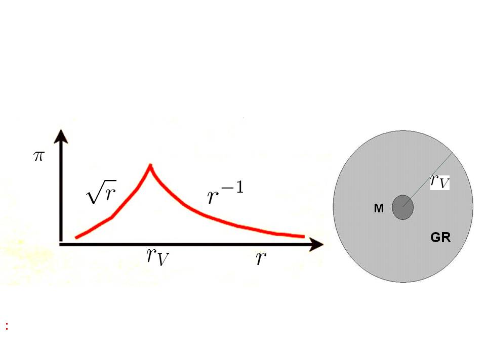
Figure 8: The figure shows Vainshtein mass screening characterized by galileon field profile for massive body of mass ${M}$. The character of non linearity crucially changes the $\pi$ profile around the body below Vainshtein radius $r_{V}$. Within this radius, the $\pi$ mediated force is negligible as compared to the Newtonian force and GR is left intact there. The modification can be felt beyond Vainshtein radius only.

V.2 Modified theories of gravity: Vainshtein screening

It is clear from the above discussion that chameleon mechanism would fail if the mass of the field is zero. How then to screen the local effects induced by such a field? There is superior field theoretic mechanism for hiding the massless degrees of freedom know as Vainshtein mechanism Vainshtein:1972sx . It does not rely on mass of the field and operates dynamically through kinetic suppression which was suggested by A. Vainshtein in 1972 to address the problem of vDVZ vanDam:1970vg ; Zakharov:1970cc discontinuity in Pauli-Fierz theory Fierz:1939ix . This mechanism can be consistently implemented through galileon field $\pi$ Nicolis:2008in ; Babichev:2013usa ; Babichev:2009us ; Gannouji:2010au ; Ali:2010gr ; Chow:2009fm ; Ali:2012cv whose Lagrangian apart from the standard kinetic term contains non-linear derivative terms of specific form. The strong non-linearities become active around a massive body below Vainshtein radius which effectively decouple the field from the source leaving GR intact there. In a space time of dimension $n$, there is a fixed number of total derivatives one can construct using $\partial_{\mu}\partial_{\nu}\pi$ correspondingly there is fixed number of galileon Lagrangians in each space time dimension.

Let us list the galileon Lagrangians in case of four dimensions Nicolis:2008in ,

$$\mathcal{L}_{1}=\pi$$ (79)

$$\mathcal{L}_{2}=-\frac{1}{2}(\partial_{\mu}\pi)^{2}$$ (80)

$$\mathcal{L}_{3}=-\frac{1}{2}(\partial_{\mu}\pi)^{2}\Box\pi$$ (81)

$$\mathcal{L}_{4}=-\frac{1}{2}(\partial_{\mu}\pi)^{2}\left[(\Box\pi)^{2}-\partial_{\mu}\partial_{\nu}\pi\partial^{\mu}\partial^{\nu}\pi\right]$$ (82)

$$\mathcal{L}_{5}=-\frac{1}{2}(\partial_{\mu}\pi)^{2}\left[(\Box\pi)^{3}-3\Box\pi(\partial_{\mu}\partial_{\nu}\pi\partial^{\mu}\partial^{\nu}\pi)+2\partial_{\alpha}\partial_{\beta}\pi\partial^{\beta}\partial^{\delta}\pi\partial_{\alpha}\partial^{\delta}\pi\right]$$ (83)

Due to the specific underlying structure from which the galileon Lagrangians can be constructed, the equations of motion for galileon field are of second order despite the higher derivative terms in the Lagrangian Nicolis:2008in . Secondly, the galileon Lagrangians are invariant under shift symmetry, $\pi\to\pi+b_{\mu}x^{\mu}+c$, in flat space time thank to which their equations of motion for can be represented as the divergence of a conserved current corresponding to the shift symmetry. Before we proceed ahead, let us remark that physics of Vainshtein mechanism is already contained in the lowest order Lagrangian $\mathcal{L}_{3}$ Chow:2009fm ; Ali:2012cv ; higher order Lagrangians add nothing to it. However, $\mathcal{L}_{3}$ alone can not give rise to de Sitter solution needed for late time cosmology; we need at least $\mathcal{L}_{4}$ to serve the purpose Gannouji:2010au ; Ali:2010gr . Since we will not address the phenomenological issues of galileon field applied to late time cosmology, we shall restrict ourselves to the lowest order galileons.

V.3 Vainshtein mechanism: Basic idea

In case of the chameleon, the mass screening relied on the effective potential Khoury:2003rn ; Khoury:2003aq ,

$$\Box\varphi=\left(V(\varphi)+\frac{\alpha}{M_{p}}\rho_{m}\varphi\right)_{,\varphi}$$ (84)

such that the mass of the field turned large in high density regime which then decouples it from the source. In case of massless field,

$$\Box\varphi=+\frac{\alpha}{M_{p}}\rho_{m}$$ (85)

chameleon ceases to work. We observe that the multiplication of the left hand side of (85) by a constant is equivalent to dividing the coupling constant $\alpha$ on the right hand side by the same constant. The latter means that enhancement of kinetic term effectively suppresses the coupling of the field to matter. However, we can not do it by hand, it should be implemented by field theoretic framework. In Vainshtein mechanism, the latter is achieved dynamically in a very intelligent manner by making use of the galileon field.
Let us briefly illustrate how kinetic suppression takes place in galileon field theory. To this end as mentioned before, it is sufficient to consider the lowest galileon Lagrangian $\mathcal{L}_{3}$ which gives rise to the following equation of motion Nicolis:2008in ; Chow:2009fm ; deser ; Ali:2012cv ,

$$\Box\pi+\frac{1}{\Lambda^{3}}[(\Box\pi)^{2}-\partial^{\mu}\partial^{\nu}\pi\partial_{\mu}\partial_{\nu}\pi]\\ =-\frac{\alpha}{M_{p}}T$$

where $\Lambda=(m^{2}M_{p})^{1/3}$ is the cut off in the effective Lagrangian and $m\sim H_{0}$. The second term on the left is non-linear which may dominate over the standard kinetic term at small scales. Indeed, for a static source of mass M($T=-M\delta^{3}(\bf{r})$), in case of spherical symmetric solution of interest to us, Eq.(V.3) acquires the following form,

$$\frac{1}{r^{2}}\frac{d}{dr}\left(r^{3}\left[(\pi^{\prime}/r)+\frac{1}{\Lambda^{3}}(\pi^{\prime}/r)^{2}\right]\right)=\frac{\alpha}{M_{p}}M\delta^{3}({r})$$ (86)

which thank to the total derivative structure of equation of motion readily integrates to

$$\left(\frac{\pi^{\prime}(r)}{r}\right)+\frac{1}{\Lambda^{3}}\left(\frac{\pi^{\prime}(r)}{r}\right)^{2}=\alpha\frac{r_{s}}{r^{3}}$$ (87)

where $r_{S}$ is the Schwarzschild radius of the massive body. We observe that at small distance the second term in the expression (87) dominates over the first which tells us that

$$\pi^{\prime}=\left(\frac{r_{S}\alpha m^{2}}{r}\right)^{1/2}$$ (88)

As a result the extra force due to galileon field is suppressed as compared to the gravitational force in the neighborhood of the massive body(see Fig.8),

$$\frac{F_{\pi}}{F_{\text{grav}}}=\left(\frac{r}{r_{V}}\right)^{3/2}<<1,~{}~{}~{}~{}r<<r_{V}$$ (89)

where the Vaishtein radius, is given by,

$$r_{V}=\left(\frac{r_{S}}{m^{2}\alpha}\right)^{1/3}$$ (90)

On the other hand, at large scales the usual kinetic term dominates over the nonlinear term and Galileon force becomes comparable to gravitational force,

$$\pi^{\prime}=\frac{{r_{S}\alpha}}{r^{2}}~{}~{}~{}\Rightarrow\frac{F_{\pi}}{F_{\text{grav}}}\sim 1$$ (91)

Let us estimate $r_{V}$ for Sun,

$$r_{V}=\frac{GM_{s}}{m^{2}}=\frac{M_{s}}{H^{2}_{0}M^{2}_{p}}\simeq 100pc$$ (92)

Hence, solar physics will not feel the presence of galileon field; any modification of gravity due the galileon degree of freedom is locally screened out due to kinetic suppression leaving GR intact in a radius much larger than the solar dimensions. For our galaxy, $r_{V}\simeq 1.2$ Mpc; the effect of galileon field might be felt at large distance through late time cosmic acceleration. It is worthwhile to note that galileon field is stable under quantum corrections unlike the chameleon.

V.4 Galileons and their higher dimensional descendants

Galileon field provides with a well defined field theory in 4 dimensions which is ghost free. On the other hand we have well defined and consistent extension of Einstein gravity in higher dimensions. In five and six dimensions, the Einstein-Hilbert action is extended by including the Gauss-Bonnet term Dadhich:2005mw , in further higher dimensions, the Lovelock structure comes into play Lovelock:1971yv ; Lovelock:1972vz . In fact, Gauss-Bonnet term is the simplest form of Lovelock Lagrangian. Thus, in each space time dimension, the consistent gravity action which leads to second order equations of motion thereby free from Ostrogradki ghosts Ostrogradski , is fixed. It is tempting to think that the two ghost free systems, the Galileon field theory in four dimensions and higher dimensional Lovelock gravity, are some way related to each other. In fact the galileon field theory in four space time dimensions is a representative of higher dimensional gravity a la Lovelock. It is interesting that dimensional reduction of $R+\alpha R^{2}_{GB}$ gives rise to lower order galileon Lagrangian, $L_{3}$, the roll of galileon field is played by the dilaton field. In what follows we briefly out line how this connection between two ghost free theories is established.

Let us consider five dimensional gravity where Einstein-Hilbert is supplemented with Gauss-Bonnet term,

$$\mathcal{S}=\int{d^{5}x\sqrt{-g^{5}}\left(R+\alpha R^{2}_{GB}\right)}$$ (93)

which is the simplest form of Lovelock theory. We then use the standard prescription to reduce the action to four dimension and use the following metric ansatz,

$$ds^{2}=g_{\mu\nu}dx^{\mu}dx^{\nu}+e^{\pi}(dx^{5})^{2}$$ (94)

where the scalar field $\pi$ appearing in the metric plays the role of the size of the extra dimensions. The dimensional reduction assuming the extra dimension to be compact, gives the following action,

$$\mathcal{S}=\int{dx^{4}\sqrt{-g}e^{\pi/2}\left(R+d_{1}(\partial_{\mu}\pi)^{2}+\alpha\left(R^{2}_{GB}+d_{2}G_{\mu\nu}\partial^{\mu}\pi\partial^{\nu}\pi+d_{3}(\partial_{\mu}\pi)^{4}+d_{4}(\partial_{\mu}\pi)^{2}\Box\pi\right)\right)}$$ (95)

The last term in the reduced action is the lowest order galileon term $L_{3}$. It is then tempting to go beyond Gauss-Bonnet, including higher order Lovelock terms. In this case, it was demonstrated in RefLG . that the dimensional reduction reproduces higher order Galileon Lagrangians. It is therefore not surprising that galileon field theory in four space time dimensions is ghost free$-$ Galileons are the representatives of higher dimensional Lovelock theory in four dimensions.

VI Glimpses of massive gravity

It is commonly believed that an elementary particle of mass $m$ and spin $s$ is described by a field which transforms according to a particular representation of Poincare group. In field theory, formulated in flat space time, mass can either be introduced by hand or generated through spontaneous symmetry breaking but general theory of relativity is not formulated as a field theory. One could naively consider the metric $g_{\mu\nu}$ as field and try to introduce mass via the invariants, $detg_{\mu\nu}$ or $Trg_{\mu\nu}$ which obviously do not serve the purpose. Hence we require a field which in some sense could represent gravity. The spin-2 field $h_{\mu\nu}$ should be relevant to gravity as it shares an important property of universality with Einstein general relativity a la Weinberg theorem . It states that the consistent quantum field theory of a spin$-$ 2 field in Minkowski space time is possible provided the field interacts with all other fields including itself with the same coupling. General theory of relativity can be thought of as an interacting theory of $h_{\mu\nu}$ field. It is therefore natural to first formulate the field theory of massive spin 2 field in flat space time and then extend it to non-linear background.

Before we proceed further, let us remember, how objects with spin-0, spin-1 and spin-2 transform under Lorentz transformation $\Lambda_{\mu\nu}$,

$$\text{ spin-0}~{}~{}~{}~{}~{}~{}~{}~{}~{}~{}~{}\phi^{\prime}=\phi$$ (96)

$$\text{spin-1}~{}~{}~{}~{}~{}~{}~{}~{}~{}~{}~{}~{}~{}A^{\prime}_{\mu}=\Lambda_{\mu}^{\alpha}A_{\alpha}$$ (97)

$$\text{spin-2}~{}~{}~{}~{}~{}~{}~{}~{}~{}~{}~{}~{}~{}h_{\mu\nu}=\Lambda^{\alpha}_{\mu}\Lambda^{\beta}_{\nu}h_{\alpha\beta}.$$ (98)

The linear massive theory of gravity of $h_{\mu\nu}$ was formulated by Fierz and Pauli in 1939 Fierz:1939ix with a motivation to write down the consistent relativistic equations for higher spin fields including spin-2 field. Let us first cast the relativistic equations of spin-0 and spin-1 fields,

$$(\Box+m^{2})\phi=0$$ (99)

$$(\Box+m^{2})A_{\mu}=0;~{}\partial_{\mu}A^{\mu}=0$$ (100)

It is important to note that the condition $\partial_{\mu}A^{\mu}=0$ is in built in the equation of motion and not imposed from outside. Indeed, from the Lagrangian of massive vector field

$$\mathcal{L}=-\frac{1}{4}F_{\mu\nu}F^{\mu\nu}-\frac{1}{2}m^{2}A_{\mu}A^{\nu}$$ (101)

follows the following equations of motion,

$$\partial_{\mu}F^{\mu\nu}+m^{2}A^{\nu}=0$$ (102)

which upon taking the divergence on both sides immediately gives us $\partial_{\mu}A^{\mu}=0$. Thus this condition for massive vector field follows from the equations of motion themselves. Massive vector field has clearly three degrees of freedom. It is important to notice that this condition can no longer be derived from the equation of motion in the $m\to 0$ limit which is consistent with the fact that we have gauge invariance in this case which allows us to get rid of two un physical degrees of freedom. Gauge invariance allows to fix the gauge which can be done in infinitely many ways. For instance we can choose the radiation gauge, $A_{0}=0$ and ${\bf\nabla}.{\bf A}$ leaving behind two transverse degrees of freedom.

Respecting relativistic invariance, we could also choose Lorentz gauge, $\partial_{\mu}A^{\mu}=0$. In massless case, this condition is imposed from out side in view of gauge freedom and this should clearly be distinguished from $\partial_{\mu}A^{\mu}=0$ occurring in case of massive vector field as a consequence of equations of motion. Lorentz gauge does not completely fix the gauge invariance. Indeed, there is a residual gauge invariance, namely, $A_{\mu}\to A_{\mu}+\partial_{\mu}\alpha$ such that $\Box\alpha=0$ which when fixed leaves behind two physical degrees of freedom.

Let us now cast the equation of motion of $h_{\mu\nu}$,

$$(\Box+m^{2})h_{\mu\nu}=0;~{}~{}\partial^{\mu}h_{\mu\nu}=0;~{}~{}h_{\mu}^{\mu}\equiv h=0$$ (103)

which tells us that massive graviton in Pauli-Fierz (PF) theory has five degrees of freedom Hinterbichler:2011tt . In accordance to our expectations, the number of degrees of freedom, $2s+1$ is 3 for massive vector field and 5 for massive graviton. The first condition on $h_{\mu\nu}$ is analogous to the case of vector field. The vanishing of trace of $h_{\mu\nu}$ is very specific to linear theory and we will come back to this point later in our discussion. The equations of motion (103) can be obtained from PF Lagrangian which has the following form,

$$\mathcal{L}_{PF}=\mathcal{L}_{m=0}-\frac{1}{2}m^{2}\left(h_{\mu\nu}h^{\mu\nu}-h^{2}\right)$$ (104)

$$\mathcal{L}_{m=0}=\frac{1}{2}\partial_{\lambda}h_{\mu\nu}\partial^{\lambda}h^{\mu\nu}+\partial_{\mu}h_{\nu\lambda}\partial^{\nu}h^{\mu\lambda}-\partial_{\mu}h^{\mu\nu}\partial_{\nu}h+\frac{1}{2}\partial_{\lambda}h\partial^{\lambda}h$$ (105)

The first term in (104) describes the massless graviton and can be obtained by considering small perturbations around flat space time, $g_{\mu\nu}\to g_{\mu\nu}+h_{\mu\nu}$ and expanding the Einstein-Hilbert Lagrangian in $h_{\mu\nu}$ up to quadratic order. It is easy to verify that the massless Lagrangian, is invariant under the following gauge transformation,

$$h_{\mu\nu}\to h_{\mu\nu}+\partial_{\mu}\xi_{\nu}+\partial_{\nu}\xi_{\mu}$$ (106)

which fixes the relative numerical values of coefficients in $\mathcal{L}_{m=0}$. The second term in (104) is the Pauli-Fierz mass term which breaks the gauge invariance (106) Hinterbichler:2011tt . The PF mass term includes two invariants that one can form using the spin-2 field. Let us notice that the mass term could in general be a linear combination of these invariants, $c_{1}h_{\mu\nu}h^{\mu\nu}-c_{2}h^{2}$; one of the multiplicative constant, say, $c_{1}$ could be absorbed in $m^{2}$ leaving the other one $c_{2}/c_{1}$, arbitrary. The PF mass terms corresponds to an intelligent tuning of the coefficient which excludes the ghost from linear theory, we shall come back to this point in the forthcoming discussion.

Recently, there was an upsurge of interests in massive gravity. A ghost free generalization of Pauli-Fierz to non linear background known as dRGT was discovered by de Rham, Gabadadze and Tolley deRham:2010ik ; deRham:2010kj . However, the motivation to go for massive gravity now is quite different from the original one. Adding mass to graviton might account for late time cosmic acceleration. For the sake of heuristic argument let us note that gravitational potential for a static point source in case of massive graviton with mass $m$ is given by, $-GMe^{-mr}/r$ with $m\sim H_{0}$ which reduces to Newtonian potential for $mr<<1$. However, at large scales such that $mr\sim 1$, adding mass to graviton gives rise to weakening of gravity. Thus the introduction of mass is effectively equivalent to repulsive effect a la cosmological constant in the standard lore. It is broadly clear that cosmological constant gets linked to graviton mass which is altogether a novel perspective. Secondly, one might have a naive feeling that since the mass of graviton is very small, the Pauli-Fierz theory would not disturb the predictions of GR in the local neighborhood. The deep scrutiny of the problem reveals that it does not hold and that the predictions Pauli-Fierz theory in the solar system are at finite difference from GR, hence the theory suffers from discontinuity problem dubbed vDVZ discontinuity vanDam:1970vg ; Zakharov:1970cc . In what follows, we shall outline the problem and expose its underlying cause.

VI.1 vDVZ discontinuity

As mentioned before, the field $h_{\mu\nu}$ universally couples to any matter source $T_{\mu\nu}$. If we expand the Einstein-Hilbert term in presence of a matter Lagrangian up to leading order in $h_{\mu\nu}$, we not only reproduce $\mathcal{L}_{m=0}$ but also obtain the coupling of the field with the source, namely, $h_{\mu\nu}T^{\mu\nu}/M_{p}$. Hence the Lagrangian of the massive spin$-$2 field interacting with matter source has the following form Hinterbichler:2011tt ,

$$\mathcal{L}=\frac{1}{2}\partial_{\lambda}h_{\mu\nu}\partial^{\lambda}h^{\mu\nu}+\partial_{\mu}h_{\nu\lambda}\partial^{\nu}h^{\mu\lambda}-\partial_{\mu}h^{\mu\nu}\partial_{\nu}h+\frac{1}{2}\partial_{\lambda}h\partial^{\lambda}h+\frac{1}{2}m^{2}\left(h_{\mu\nu}h^{\mu\nu}-h^{2}\right)+\frac{1}{M_{p}}h_{\mu\nu}T^{\mu\nu}$$ (107)

In order to understand the problem, we need to compute the scattering amplitude of two matter sources for which we need the expressions of propagators for massless and massive gravitons(Fig.9). These propagators can be written using the free part of (138), skipping details, we quote their expressions Hinterbichler:2011tt ,

$$\mathcal{D}^{0}_{\alpha\beta,\rho\sigma}=-\frac{1}{k^{2}}\Big{[}\frac{1}{2}\left(\eta_{\alpha\rho}\eta_{\beta\sigma}+\eta_{\alpha\sigma}\eta_{\beta\rho}\right)-\frac{1}{2}\eta_{\alpha\beta}\eta_{\rho\sigma}\Big{]}$$ (108)

$$\mathcal{D}^{m}_{\alpha\beta,\rho\sigma}=-\frac{1}{k^{2}+m^{2}}\Big{[}\frac{1}{2}\left(\eta_{\alpha\rho}\eta_{\beta\sigma}+\eta_{\alpha\sigma}\eta_{\beta\rho}\right)-\frac{1}{3}\eta_{\alpha\beta}\eta_{\rho\sigma}\Big{]}$$ (109)

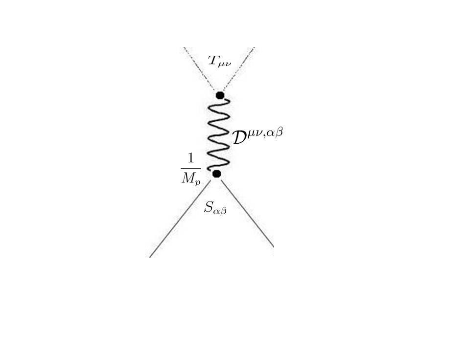
Figure 9: Tree level scattering of two matter sources $T_{\mu\nu}$ and $S_{\alpha\beta}$ which couple with the universal coupling constant, $1/M_{p}$ and $\mathcal{D}^{\mu\nu,\alpha\beta}$ is the propagator of massive(massless) graviton

It should be noticed that the numerical coefficients of last terms in (108) $\&$ (109) are different. The fact, that a massive graviton has five degrees of freedom whereas massless graviton has only two, is reflected in the expressions of their propagators. Let us now compute the tree level amplitude of scattering of two matter sources $S_{\alpha\beta}$ and $T_{\alpha\beta}$ in massless and massive gravity. The corresponding amplitudes are given by

$$A^{(0)}=-\frac{8\pi G}{k^{2}}\left(S_{\mu\nu}T^{\mu\nu}-\frac{1}{2}ST\right)$$ (110)

$$A^{(m)}=-\frac{8\pi G}{k^{2}+m^{2}}\left(S_{\mu\nu}T^{\mu\nu}-\frac{1}{3}ST\right)$$ (111)

In case of two static sources with masses, $M_{1}$ and $M_{2}$, we have,

$$A^{(0)}=-\frac{4\pi}{k^{2}}GM_{1}M_{2}$$ (112)

$$A^{(m)}=-\frac{4\pi}{k^{2}+m^{2}}\left(\frac{4}{3}G\right)M_{1}M_{2}$$ (113)

In mass going to zero limit $m\to 0$, the amplitude $A^{(m)}$ does not reduce to $A^{(0)}$ as opposed to our naive expectations. Massive gravity in $m\to 0$ goes to a theory in which $G$ gets replaced by $4G/3$. We therefore conclude that linear massive gravity is at finite difference from $GR$ and hence inconsistent. In case we deform the parameters in a theory and then switch off the deformation, logical consistency demands that the modified theory should reduce to the original set up which does not happen in case of PF theory.

Before addressing the problem, we have to clearly understand the underlying reason for vDVZ discontinuity. We shall present heuristic arguments without going into detailed exposition of the problem. First of all, we note that the procedure of taking limit should be legitimate, it should preserve the degrees of freedom. The correct frame work of carrying out such a program is provided by Stukelberg formalism Stueckelberg:1957zz ; Ruegg:2003ps which reinstate the gauge invariance broken by Pauli-Fierz mass term. After taking then the $m\to 0$ limit, we have to worry about the three extra degrees of freedom. In case of massive vector field, the extra (longitudinal) degree of freedom gets decoupled from the system thereby no discontinuity problem. Let us recall that in case of the Yang-Mills, say SU(2), theory, if one of vector bosons happens to be in the longitudinal state, it can be decoupled from the system whereas the other two can not be; in this case one requires Higgs field to address the problem. It is therefore quite possible that the extra degrees of freedom in case of gravity might not decouple from the source. Let us write the following decomposition for $h_{\mu\nu}$,

$$h_{\mu\nu}=h^{t}_{\mu\nu}+\partial_{\mu}A_{\nu}+\partial_{\nu}A_{\mu}+\partial_{\mu}\partial\nu\phi$$ (114)

Such a decomposition can be understood either from group representation or at the level of Lagrangian formalismHinterbichler:2011tt . In $m\to 0$ limit, $h^{t}_{\mu\nu}$, $A_{\mu}$ represent two transverse degrees of massless graviton, two degrees of freedom of massless vector field whereas $\phi$ is the longitudinal component of $h_{\mu\nu}$. Let us argue that $A_{\mu}$ will not couple with the given conserved source $T_{\mu\nu}$. Its coupling could be of the form, $(\partial_{\mu}A_{\nu}+\partial_{\nu}A_{\mu})T^{\mu\nu}$; by integration of parts, we can through the derivative on $T_{\mu\nu}$ to discard this possibility. As for the longitudinal component, the only possibility is that it couples with the trace of $T_{\mu\nu}$ as $\phi T$. The detailed investigations reveal that indeed this is the case and the coupling constant is same as in case of the massless gravitonHinterbichler:2011tt . In massive gravity, there is an extra contribution to the scattering amplitude due to the exchange of scalar degree which is of the same order as the amplitude in Einstein gravity. This could also be noticed by rewriting the propagator of massive graviton in the following form,

$$\mathcal{D}^{m}_{\alpha\beta,\rho\sigma}=-\frac{1}{k^{2}+m^{2}}\Big{[}\frac{1}{2}\left(\eta_{\alpha\rho}\eta_{\beta\sigma}+\eta_{\alpha\sigma}\eta_{\beta\rho}\right)-\frac{1}{2}\eta_{\alpha\beta}\eta_{\rho\sigma}\Big{]}+\frac{1}{6}\frac{\eta_{\alpha\beta}\eta_{\rho\sigma}}{k^{2}+m^{2}}$$ (115)

where the first term represents transverse part of massive spin-2 field propagator whereas the second part is nothing but propagator of massive scalar field. It is therefore clear that the theory under consideration can not reduce to GR, see Fig.10).

We exposed the underlying reason of the discontinuity which is generic to linear massive gravity a la Pauli-Fierz . How do we cure this problem. The irony is that again we deal with an extra scalar field similar to the chameleon theory. In that case we implemented chameleon screening which is not viable in this case as the scalar degree of freedom is massless. It was pointed out by Vainshtein in 1972 that the linear approximation breaks down in the neighborhood of a massive body below certain radius $r_{V}$ and that the non linear effects screen out any modification to gravity below $r_{V}$ leaving GR intact there. It tempting to think that the longitudinal degree of freedom could be galileon though this aspect of Vinshtein screening became known very recently. Actually, this mechanism is in built in DGP Dvali:2000hr where lowest order Galileon term occurs in the so called decoupling limit. The connection of Galileon to screening was the central point in the formulation of dRGT. Before we discuss this development, let us show that PF theory will have ghost if we try to extend it to non linear background or we break the Pauli-Fierz tuning. In both the cases, we end up with equations of motion of order higher than second which inevitably leads to Ostrogradki instability or ghosts.

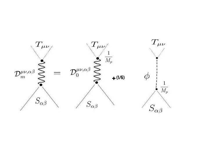
Figure 10: Scattering of two matter sources $T_{\mu\nu}$ and $S_{\alpha\beta}$ at tree level in massive gravity. The process in the $m\to 0$ limit is represented by the exchange of massless graviton as usual(first diagram on right) plus an extra interaction mediated by the longitudinal mode $\phi$ which couples with the matter sources with the universal coupling of GR.

It is not by chance that first evolution equation $-$ the Newton’s second law is a second order equation. We should wonder why dynamical equations that we come across are of second order. The answer to this profound question was provided by Ostrogradski. If the higher order time derivative Lagrangian is non-degenerate, there is at least one linear instability in the Hamiltonian of this system which means that Hamiltonian is unbounded from below. In general, if the Lagrangian is not invertible, there are constraints in the system and Ostrogradski theorem does not hold; such a system might be stable. The Ostrogradski Lagrangian essentially leads to equations of motion of higher order than second. While quantizing a system whose Hamiltonian is unbounded from below, one encounters negative norm states dubbed ghosts Ostrogradski .

VI.2 Ostrogradski $(ghosts)$ instability

In order to see how Ostrogradski instability occurs, let us for simplicity consider a Lagrangian, $\mathcal{L}(q,\dot{q})$ with the standard equation of motion(see Ref.Woodard , an excellent review on this theme),

$$\frac{\partial\mathcal{L}}{\partial q}-\frac{d}{dt}\frac{\partial\mathcal{L}}{\partial\dot{q}}=0$$ (116)

The Lagrangian is non degenerate if $\frac{\partial^{2}\mathcal{L}}{\partial\dot{q}^{2}}\neq 0$ which simply means that $\frac{\partial\mathcal{L}}{\partial\dot{q}}$ depends upon $\dot{q}$. In this case, Lagrangian equation can be cast in the form of Newton’s second law ,

$$\ddot{q}=f(q,\dot{q})$$ (117)

whose unique solution $q(t)$ requires the knowledge of two initial conditions on $q(t)$ and $\dot{q}(t)$. We can then transform from configuration space $(q,\dot{q})$ to phase space $(q,p)$ by defining the canonical momentum $p$,

$$p=\frac{\partial\mathcal{L}}{\partial\dot{q}}$$ (118)

which thank to the non degeneracy of the Lagrangian allows us to express, $\dot{q}$ in terms of $q$ and $p$. One then sets up the Hamiltonian

$$H(q,p)=p\dot{q}-\mathcal{L}(q,\dot{q})\to dH=\dot{q}dp-\dot{p}dq$$ (119)

from which reads out the Hamiltonian equations,

$$\dot{q}=\frac{\partial H}{\partial p},~{}~{}~{}\dot{p}=-\frac{\partial H}{\partial q}$$ (120)

that are equivalent to Lagrangian equation. Things would qualitatively change in case the Lagrangian depends on time derivatives higher than one. Indeed, let us consider the Lagrangian, $\mathcal{L}(q,\dot{q},\ddot{q})$ for which the equation of motion has the following form,

$$\frac{\partial\mathcal{L}}{\partial q}-\frac{d}{dt}\frac{\partial\mathcal{L}}{\partial\dot{q}}+\frac{d^{2}}{dt^{2}}\frac{\partial\mathcal{L}}{\partial\ddot{q}}=0$$ (121)

In this case, the non degeneracy of the Lagrangian would imply that $\frac{\partial\mathcal{L}}{\partial\ddot{q}}$ depends upon $\ddot{q}$. Lagrangian equation (121) then gives rise to following fourth order differential equation,

$$\ddddot{q}(t)=f(q,\dot{q},\ddot{q},\dddot{q})$$ (122)

Uniqueness of the solution $q(t)$ of (122) would require the extra information on the initial values of $\ddot{q}$ and $\dddot{q}$ in addition to $(q_{0},\dot{q}_{0})$. The extra information brings in instability in the system or ghost. Indeed, analogous to the standard case, we have four canonical variables in this case. Following Ostrogradski, we choose them as,

$$q_{1}=q,~{}~{}~{}p_{1}=\frac{\partial\mathcal{L}}{\partial\dot{q_{1}}}-\frac{d}{dt}\frac{\partial\mathcal{L}}{\partial\ddot{q}}$$ (123)

$$q_{2}=\dot{q},~{}~{}~{}p_{2}=\frac{\partial\mathcal{L}}{\partial\ddot{q}}$$ (124)

Non degeneracy of the Lagrangian means that we can express $\partial\mathcal{L}/\partial\ddot{q}$ through $q_{1},q_{2}$ and $p_{2}$. We can then set up the Ostrogradski Hamiltonian,

$$H=p_{1}\dot{q}_{1}+p_{2}\dot{q}_{2}-\mathcal{L}(q_{1},q_{2},p_{2})=p_{1}q_{2}+p_{2}\dot{q}_{2}-\mathcal{L}(q_{1},q_{2},p_{2})$$ (125)

The Hamiltonian equations for (125) analogous to the standard case have the similar form,

$$\dot{q}_{i}=\frac{\partial H}{\partial p_{i}};~{}~{}\dot{p}=-\frac{\partial H}{\partial q_{i}},~{}~{}i=1,2$$ (126)

and it is not difficult to check that they are equivalent to (121) and also reproduce phase space transformation. The Hamiltonian (125) acquires a strange piece with respect to the canonical momentum $p_{1}$ which primarily appears due to the higher derivative term in the Lagrangian. As the Hamiltonian (125) is linear in $p_{1}$, the dynamical system under consideration is unstable in half of the phase space. Bringing in one higher derivative brings in one bad degree of freedom. In case, the Lagrangian contains $n$ higher derivative and satisfies the condition of non degeneracy, the Ostrogradski Hamiltonian would be linear in all the $n$ momenta and hence not bounded from below along $n$ directions. The Ostrogradski instability is a very generic phenomenon which can not be cured by passing to the quantum theory. Efforts of quantizing such a system gives rise to the negative norm states or ghosts. By adding constraints to the system, one can not get rid of these ghosts. One should either avoid higher order equations or ensure that ghosts do not occur below the cut off in the effective theory of interest hoping that UV completion would address the problem.

VI.3 Ghosts in massive gravity

The choice of PF mass term is very generic, as mentioned before, the violation of Pauli-Fierz tuning leads to ghost. Indeed let us consider the following mass term,

$$\mathcal{L}_{m}=-\frac{1}{2}m^{2}\left(ah_{\mu\nu}h^{\mu\nu}-h^{2}\right)$$ (127)

where a is constant. The Lagrangian $\mathcal{L}$ is invariant under the following transformation pattern like a gauge transformation,

$$h_{\mu\nu}\to h_{\mu\nu}+\partial_{\mu}A_{\nu}+\partial_{\nu}A_{\mu}+\partial_{\mu}\partial\nu\phi$$ (128)

but the massive term breaks this invariance and we get an additional term for $\phi$ field(vector field is not of interest here) that includes higher derivative term $(\Box\phi)^{2}$. As a result the $\phi$ Lagrangian we deal with in this case is of the following type

$$\frac{m^{2}}{2d^{2}}(\left(\Box\phi\right)^{2}-\frac{1}{2}(\partial_{\mu}\phi)^{2},~{}d^{2}=\frac{1}{2(a-1)}$$ (129)

The first term in this expression is dangerous, this is the higher order derivative term which leads to ghost in accordance with the Ostrogradski theorem. Lets us compute the mass of the ghost. One can easily check that (129) is equivalent to the following LagrangianCreminelli:2005qk ,

$$\mathcal{L}_{g}=-\frac{1}{2}(\partial_{\mu}\phi)^{2}-m^{2}\partial_{\mu}\chi\partial^{\mu}\phi-\frac{1}{2}m^{2}d^{2}\chi^{2}$$ (130)

where $\chi$ is an auxiliary field. Varying (130) with respect to $\chi$, one finds, $\chi=\frac{1}{d^{2}}\Box\phi$ and invoking it back into (130), one reinstates the original expression (129). Next, changing the variable $\phi\to\phi^{\prime}-m^{2}\chi$, one can diagonalize (130),

$$\mathcal{L}_{g}=-\frac{1}{2}(\partial_{\mu}\phi^{\prime})^{2}+(\partial_{\mu}\chi)^{2}-\frac{1}{2}m^{2}d^{2}\chi^{2}$$ (131)

It is now clear that (129) describes two degrees of freedom, one of which ($\chi$) is ghost and its mass is given by

$$m^{2}_{ghost}=\frac{m^{2}}{2(a-1)}$$ (132)

which is infinite in case $a=1$, thereby ghost does not propagate in Pauli-Fierz theory, it is led to sleep in its grave. Hence PF tuning is generic for the theory to be a consistent field theory.
Let us now check that ghost dubbed Boulware-Deser ghost will wake up if we try to naively extend the theory to non linear background Boulware:1974sr . In this case the Einstein equations take the following formCreminelli:2005qk ,

$$G_{\mu\nu}-\frac{1}{2}m^{2}\Big{[}\left(h_{\mu\nu}-h\eta_{\mu\nu})+\mathcal{O}(h^{2}_{\mu\nu}\right)\Big{]}=0$$ (133)

where we have allowed non linearity in the mass term also. Gauge invariance then ensures the Bianchi identity

$$\nabla^{\mu}(h_{\mu\nu}-h\eta_{\mu\nu})+\mathcal{O}(h^{2}_{\mu\nu})=0$$ (134)

which forces the trace of $G_{\mu\nu}$

$$G^{\mu}_{\mu}(L)=2\partial^{\mu}\partial^{\nu}(h_{\mu\nu}-h\eta_{\mu\nu})$$ (135)

to vanish at the linear order. This in turn follows from (133) at the linear level that $h=0$. It is therefore clear that the constraint that trace of $h_{\mu\nu}$ vanishes is specific to linear theory. If we allow non linearity of lowest order, instead of constraint we get an equation,

$$\mathcal{O}(\partial^{2}h^{2}_{\mu\nu})-\frac{1}{2}m^{2}\left(-3h+\mathcal{O}(h^{2}_{\mu\nu})\right)=0$$ (136)

and as a consequence, Boulware-Deser ghost becomes alive and begins to propagate. Now we get into a dilemma, linear theory has no ghost but plagued with vDVZ discontinuity which can be resolved by extending the theory to non linear background but the latter makes the ghost alive. At the onset it sounds like a no go theorem. This is the reason why massive gravity did not progress for a long time. Very recently, a non linear generalization of PF theory was proposed.

VII $dRGT$ at a glance

The above discussion shows that that the extension of PF theory to non linear background leads to ghost. Question then arises, can we generalize PF mass term higher order than second such that ghost does not occur. The answer is yes$-$ a very specific structure can do that and the framework is known as $dRGT$ deRham:2010ik ; deRham:2010kj . Since the PF mass term breaks gauge invariance, the first step is to reinstate the general covariance which is done by using the Stuckelberg formalism Stueckelberg:1957zz ; Ruegg:2003ps . One needs to replace $h_{\mu\nu}$ by a general covariant tensor $H_{\mu\nu}$; we need four scalar fields, $\phi_{a},a=1,4$,

$$H_{\mu\nu}=g_{\mu\nu}-\partial_{\mu}\phi^{a}\partial_{\nu}\phi^{b}\eta_{ab}$$ (137)

An important comment about reinstating the general covariance in (137) is in order. We could replace flat metric $\eta_{ab}$ in (137) by any other metric to serve the purpose. But changing metric would change the underlying physics. There is no fundamental principle that can allow us to make a particular choice except considerations based upon simplicity or phenomenology. One way out is to turn the reference metric into dynamical one and opt for bi-gravity theories. Let us also note that $\phi^{a}$ is scalar under diffeomorphizm but transforms as a vector under Lorentz transformation. The PF mass term then becomes,

$$-\frac{m^{2}M^{2}_{P}}{8}g^{\mu\nu}g^{\rho\sigma}\left(H_{\mu\rho}H_{\nu\sigma}-H_{\mu}H_{\rho\sigma}\right)$$ (138)

which is the right object to cast in the non linear background,

$$\mathcal{L}=\frac{M^{2}_{p}}{2}R-\frac{m^{2}M^{2}_{P}}{8}g^{\mu\nu}g^{\rho\sigma}\left(H_{\mu\rho}H_{\nu\sigma}-H_{\mu}H_{\rho\sigma}\right)+\mathcal{L}_{m}$$ (139)

where we have added the matter Lagrangian. Let us notice that in the unitary gauge, $\phi^{a}=x^{a}$, (138) reduces to PF mass term. One can go beyond unitary gauge and write helicity decomposition for $\phi^{a}$ using canonical fields,

$$\phi^{a}=x^{a}+{A^{a}}+\eta^{ab}{\partial_{b}\phi}$$ (140)

As mentioned before, we can ignore the vector field and focus on helicity zero component,

$$H_{\mu\nu}={h_{\mu\nu}}+2\partial_{\mu}\partial_{\nu}\phi-\eta^{\alpha\beta}\partial_{\mu}\partial_{\nu}\phi\partial_{\alpha}\partial_{\beta}\phi$$ (141)

which is justified in a limit known as decoupling limit.

VII.1 Decoupling limit

The decoupling limit is some sort of high energy limit. This limit is very helpful in counting the degrees of freedom in massive gravity and provides with a valid framework to discuss the mass screening in the local environment.

In this limit one is dealing with energies much higher than the mass of the graviton ArkaniHamed:2002sp ; Luty:2003vm ; deRham:2010ik ; deRham:2010kj ,

$$M_{p}\to\infty,~{}m\to 0,~{}T=\infty,~{}\Lambda={\rm fixed},~{}~{}\frac{T}{M_{p}}={\rm fixed}$$ (142)

In the decoupling limit, the dominant $\phi$ interactions survive and Einstein-Hilbert action linearizes in $h_{\mu\nu}$ such that (139) reduces to the following deRham:2010ik ; deRham:2010kj ; Hinterbichler:2011tt ,

$$\mathcal{L}=\mathcal{L}_{m=0}-\frac{1}{4}F_{\mu\nu}F^{\mu\nu}-3(\partial_{\mu}\phi)^{2}+\frac{1}{\Lambda_{5}^{5}}\left[(\Box\phi)^{3}-\Box\phi\partial_{\mu}\partial_{\nu}\phi)^{3}\right]+\frac{1}{M_{p}}h_{\mu\nu}T^{\mu\nu}$$ (143)

where $\Lambda_{5}=(m^{4}M_{p})^{1/5}$ is the cut off in the theory. A comment about the decoupling Lagrangian (143) is in order. We first carry out expansion around the unitary gauge (140) and the expansion around flat space time, $g_{\mu\nu}=\eta_{\mu\nu}+h_{\mu\nu}$.

The Einstein-Hilbert action expanded to quadratic order in $h_{\mu\nu}$ gives rise to $M^{2}_{p}/4$ multiplied by the quadratic piece in $h_{\mu\nu}$. The expansion of matter Lagrangian produces, $h_{\mu\nu}T^{\mu\nu}/2$. Once we opt for the canonical fields, $h_{\mu\nu}\to 2h_{\mu\nu}/M_{p}$, we obtain $\mathcal{L}_{m=0}$ from Einstein-Hilbert term plus the last term in (143) from $h_{\mu\nu}T^{\mu\nu}/2$. As for the higher order terms in $h_{\mu\nu}$, they drop out in the decoupling limit. Hence Einstein-Hilbert action linearizes in the decoupling limit.

Next by invoking the helicity decomposition in the mass term and using the canonical normalization for $A_{\mu}\to 2A/mM_{p}$ and $\phi\to 2\phi/m^{2}M_{p}$, we obtain other terms in (143) in the decoupling limit. Let us first note that $\phi$ coupling with matter source survives the decoupling limit whereas the vector field coupling does not. The non linear derivative $\phi$ self coupling is controlled by the cut off $\Lambda_{5}$ which is precisely the scale at which non linearities become important. The non linear coupling is responsible for restoring GR below Vainshtein radius defined by the cut off. Unfortunately , the higher order derivative terms in (143) are dangerous; they do not belong to the class of galileons and give rise to Ostrogradski ghost. Thus, $\phi$ acquires an additional degree of freedom, a ghost which precisely cancels the contribution of longitudinal degree of freedom and restores $GR$ within Vainshtein radius in the non linear backgroundHinterbichler:2011tt . We thus solve $vDVZ$ discontinuity but a ghost gets introduced in the process which is unacceptable. It would have been really remarkable, had the higher order derivative $\phi$ Lagrangian in the decoupling limit were a galileon Lagrangian!. The question then arises, can we include higher order terms in the Lagrangian (139) such that ghosts do not occur. We consider the following generalization deRham:2010kj ,

$$\mathcal{L}=\frac{M_{p}^{2}}{2}R-\frac{1}{8}m^{2}M^{2}_{p}\mathcal{U}(H_{\mu\nu},g_{\mu\nu})$$ (144)

The expansion of $\mathcal{U}$ in $H_{\mu\nu}$ in its lowest order will produce (139). However, in the nth order it will give rise to terms like $(\partial^{2}\phi)^{2n}$ and would lead to ghosts in general in view of Ostrogradski theorem. Hence, $\mathcal{U}$ should be chosen in a very specific and clever manner such that in the decoupling limit, the non linear Lagrangian either reduces to total derivatives or to the galileons. It is easier first to check it in the decoupling limit and then generalize the result beyond this limit.

The goal is achieved if the structure of $\mathcal{U}$ is such that when expanded in $h_{\mu\nu}$,

$$\mathcal{U}_{M_{p}\to\infty}\equiv\mathcal{U}_{h_{\mu\nu}\to 0}=\mathcal{U}_{0}+F_{G}(\phi)h_{\mu\nu}+...$$ (145)

the zeroth order term, $\mathcal{U}_{0}$ is a total derivative and does not reflect on the equations of motion. The first order correction is important in the expansion (145), the only option for it not to be dangerous is that $F_{G}(\phi)h_{\mu\nu}$ should be represented by a galileon field alone once the Lagrangian is diagonalized thereby ghost free despite being higher derivative. As for the higher order terms in the expansion (145), the same should keep repeating. Actually, $dRGT$ operates with a specially chosen form of $\mathcal{U}$ which satisfies this criteria. It becomes cumbersome to tackle the higher order terms in the expansion of $\mathcal{U}$; one can then work in the unitary gauge to confirm that the sixth degree of freedom is indeed absent in $dRGT$.
Let us now specify the form of $\mathcal{L}$,

$$\mathcal{S}_{\rm{mass}} =\frac{m^{2}M_{Pl}^{2}}{8}\int{\rm d}^{4}x\sqrt{-g}~{}\Bigl{[}\mathcal{U}_{2}+\alpha_{3}\mathcal{U}_{3}+\alpha_{4}\mathcal{U}_{4}\Bigr{]}$$ (146)

In action (146), $\alpha_{3}$, $\alpha_{4}$ are two arbitrary parameters and $U_{i}$ are specific polynomials of the matrix

$$\mathcal{K}^{\mu}_{\nu}=\delta^{\mu}_{\nu}-\sqrt{g^{\mu\alpha}\partial_{\alpha}\phi^{a}\partial_{\nu}\phi^{b}\eta_{ab}},$$ (147)

given by,

$$\mathcal{U}_{2} =4([\mathcal{K}]^{2}-[\mathcal{K}^{2}])$$ (148)

$$\mathcal{U}_{3} =[\mathcal{K}]^{3}-3[\mathcal{K}][\mathcal{K}^{2}]+2[\mathcal{K}^{3}]$$ (149)

$$\mathcal{U}_{4} =[\mathcal{K}]^{4}-6[\mathcal{K}]^{2}[\mathcal{K}^{2}]+3[\mathcal{K}^{2}]^{2}+8[\mathcal{K}][\mathcal{K}^{3}]-6[\mathcal{K}^{4}].$$ (150)

In (147), $\eta_{ab}$ (Minkowski metric) is a reference metric and $\phi^{a}(x)$ are the Stückelberg scalars introduced to restore general covariance ArkaniHamed:2002sp . Let us comment on the choice of the action. We first note that in the decoupling limit, the specially constructed matrix, $\mathcal{K}|_{h_{\mu\nu}\to 0}\to\partial_{\mu}\partial_{\nu}\phi$ and by virtue of special construction (148), all the $\mathcal{U}$ turn into total derivatives in this limit. Actually, $\mathcal{U}_{i},i=1,3$ are only non trivial total derivatives in four dimensions one can (uniquely) construct from $\partial_{\mu}\partial_{\nu}\phi$ The fact that $\mathcal{U}_{2}$ reduces to total derivative in the zero order of the decoupling limit speaks of the success of PF theory. Next, one can show that galileons occur in the first order correction when we expand the mass term in $h_{\mu\nu}$ and diagonalize the Lagrangian using the conformal transformation on $h_{\mu\nu}$. This ensures that local physics is taken care of by the Vainshtein effect and no ghost occurs in the decoupling limit. It can be demonstrated that this result remains valid beyond the decoupling limit.

VII.2 FRW cosmology: Difficulties of $dRGT$

We consider a flat Friedmann-Robertson-Walker (FRW) metric of the formmassc

$${\rm d}s^{2}=g_{\mu\nu}dx^{\mu}dx^{\nu}=-N(t)^{2}dt^{2}+a^{2}(t)\delta_{ij}dx^{i}dx^{j}$$ (151)

while for the Stückelberg scalars we consider the ansatz

$$\phi^{0}=f(t),~{}~{}~{}\phi^{i}=x^{i}.$$ (152)

In this case the Einstein-Hilbert action and the action 146 become:

$$\mathcal{S}_{\rm{EH}} =-3M_{Pl}^{2}\int{\rm d}t\Bigl{[}\frac{a\dot{a}^{2}}{N}\Bigr{]}$$ (153)

$$\mathcal{S}_{\rm{mass}} =3m^{2}M_{Pl}^{2}\int{\rm d}ta^{3}\Bigl{[}NG_{1}(\xi)-\dot{f}aG_{2}(\xi)\Bigr{]}$$ (154)

where we have defined

$$G_{1}(\xi) =(1-\xi)\Bigl{[}2-\xi+\frac{\alpha_{3}}{4}(1-\xi)(4-\xi)+\alpha_{4}(1-\xi)^{2}\Bigr{]}$$ (156)

$$G_{2}(\xi) =\xi(1-\xi)\Bigl{[}1+\frac{3}{4}\alpha_{3}(1-\xi)+\alpha_{4}(1-\xi)^{2}\Bigr{]};\xi=\frac{1}{a}$$ (157)

Variation with respect to $N$, setting $N=1$ at the end, leads to the first Friedmann equation

$$3M_{Pl}^{2}H^{2}={\rho_{m}+\rho_{r}-3m^{2}M_{p}^{2}G_{1}}$$ (158)

Variation with respect to $f$ gives the constraint equation

$$\frac{d}{dt}\left(m^{2}a^{4}G_{2}(a)\right)=0~{}\to G_{2}(a)=\frac{C}{a^{4}}$$ (159)

where $C$ is a constant of integration. The constraint equation is problematic as it implies that $a=const$. We can invoke spatially non flat geometry and obtain a viable background dynamics. However, the latter turn out to be unstable under perturbationsma . Even if these branches were stable, the absence of spatially flat geometry would mean point towards some underlying problem of $dRGT$. There are clearly three ways to handle the problem: (1) We may adhere to the point of view that the mass of graviton is strictly zero and abandon the efforts to look for consistent theory of massive gravity. (2) Perhaps the easiest way out is to modify $dRGT$ at the level of cosmology, say by making the mass of graviton a field variable by replacing $m\to V(\psi)$ or by introducing a dilaton field which by itself can not lead to a fundamental ideadilaton . This is similar to curing a wound from out side without providing an internal therapy. The bi-metric theories and the models of massive gravity based upon Lorentz violations could be a serious option in this categorydefa ; hr ; rubakov . (3) If we adopt a conservative and pragmatic view , we might claim that $dRGT$ is a correct theory. It predicts a generic anisotropy in the universe and points towards the violation of cosmological principle. The recent investigations on optical polarizations, CMB quadrupole and octopole and the study of radio sources point towards a large scale anisotropy with the preferred axis(see, Ref.jain and references therein). We may therefore abandon the FRW cosmology and opt for an anisotropic background. (4) The most challenging way out is to modify $dRGT$ at the fundamental level. Let us note that bi-gravity theories sound promising with healthy FRW cosmology at late times. Unfortunately, the theory runs into difficulties in the early universemaeda .

VIII summary and outlook

In this brief review we presented a broad account of standard lore of cosmic acceleration a la dark energy and large scale modification of gravity. Given the observational constraints and difficulties associated with model building of dynamical dark energy, it would be fair to say that cosmological constant emerges in a stronger position. There are three distinguished features which make it a celebrity. First, it is the integral part of Einstein gravity and requires no adhoc assumption for its introduction. In fact, it makes classical Einstein gravity complete in four dimensions. Secondly, it provides with the simplest possibility to describe late time cosmic acceleration. Last but not least, it is consistent with all the observations and performs better than models of dynamical dark energy. Given the present data which is quite accurate at the background level, we can not distinguish cosmological constant from quintessence or large scale modification ; the needle of hope points towards the cosmological constant as the source of cosmic acceleration. At present, the cosmology community tacitely agrees that at the background level there is nothing but cosmological constant. However,one should admit that there are difficult theoretical issues associated with cosmological constant. Its incredibly small value and the absence of a generic symmetry at the associated energy scales to protect it from quantum corrections make the problem most challenging in theoretical physics.
With a hope to alleviate the cosmological constant problem, a variety of scalar field models were introduced. We have here presented basic features of cosmological dynamics of scalar fields. In our opinion, scalar field models can not address the said problem. A fundamental scalar field is plagued with naturalness problem thereby one problem translates into another one of similar naturesmyr .
There is a school of thought in cosmology which preaches the necessity of paradigm shift, namely, that large scale modification of gravity might account for late time cosmic acceleration. As we pointed out earlier, the generic modifications amount to extra degrees of freedom expected to complement Einstein gravity at large scales. The tough challenges of these scenarios are related to local physics constraints. In case the extra degrees are massive, the required accuracy of their screening a la chameleon mechanism in the local neighborhood leaves no scope for large scale modification to account for late time cosmic acceleration.
As for the massless degrees, they should be represented by galileon field which can implement Vainshtein screening. Galileon field appears in the decoupling limit in massive gravity. We have briefly described the connection of galileon field to their higher dimensional descendent, the Lovelock gravity which leaves no surprise for them to be ghost free. However, the fact that they can protect local physics in the decoupling limit is a big bonus for galileons. There are, however, issues here which need attention. Galileons are legitimate representatives of a profound structure in higher dimensions$-$ the Lovelock theory. The linkage of these two systems may be established through dimensional reduction $-$ a well defined procedure to establish contact with four dimension we live in. It is really surprising where galileon field inherit superluminality from. This feature can not come from Lovelock structure, may be it is induced from reduction process! One should also ponder upon the connection (if any) of generalized galileon dubbed Hordenski system to higher dimensions.
‘ Galileon field serves as a fundamental building block for non linear ghost free massive gravity. Interestingly, kicking out ghost from the theory brings in superluminality, an inherent feature of galileons. Even if we close our eyes on causality issues, the ghost free massive gravity a la $dRGT$ miserably fails in cosmology it was meant for. In our opinion, adding yet new degree to the set up, such as a dilaton, at cosmology level defeats the original motivation of the theory. In our description of massive gravity, we avoided technical issues and often resorted to heuristical arguments based upon physical perceptions. And this is consistent with the motivation of the review to convey the basic ideas of the theme under consideration to a wider audience.
There is a beautiful field theoretic framework in the background of the non linear ghost free massive gravity and we believe that such a beauty can not go for waist. We believe that some fundamental idea would resolve the underlying difficulty, may be, something similar to the Higgs mechanism that salvaged the standard model of particle physics.
On the observational front, we expect to distinguish between Einstein gravity(with cosmological constant) and modified schemes (f(R), DGP etc) in future surveys. On theoretical grounds, the former emerges cleaner than any large scale modification. As for the modified theories, despite inherent difficulties, non linear massive gravity deserves attention due to its generic features. It links cosmological constant to the mass of a fundamental particle, the graviton and provides with some mechanism of degravitaion. At present, we do not know a consistent model of large scale modification of gravity. In such situation one might opt for an effective description containing a single scalar field of most general nature non-minimally coupled to matter. We believe that future surveys of large scale structure would reveal if there is physics beyond $\Lambda$CDM.
Clearly, the phenomenon of late time cosmic acceleration is far from being understood. This is certainly the puzzle of the millennium and it is therefore not surprising that there is no easy solution to this problem. Observational missions are in full swing in cosmology at present and there is no doubt that interesting times are ahead for theoreticians as well as for observers.

IX Acknowledgements

We are indebted to W. Hossain, R. Gannouji , S. Mukohyama and Safia Ahmad for taking pain in reading through the manuscript and pointing out corrections and making suggestions for improvement. We thank N. Dadhich, S. Jhingan, J. V. Narlikar, S. Odintsov, T. Padmanabhan, V. Sahni , A. A. Sen, S. Tsujikawa and Yi Wang for comments and fruitful discussions. MS thanks R. Kaul for fruitful discussions on the stability of fundamental scalar under radiative corrections. He thanks R.U. Khan for his help in drawing figures. He also thanks Eurasian International Center for Theoretical Physics(Eurasian National University, Astana) for hospitality where the work on the review was completed.

References

- (1) E. Hubble, Proc. Nat. Acad. Sci. 15, 168 (1929).
- (2) G. Gamow, “Expanding universe and the origin of elements,” Phys. Rev. 70, 572 (1946). R. A. Alpher, H. Bethe and G. Gamow, “The origin of chemical elements,” Phys. Rev. 73, 803 (1948). R. A. Alpher, J. W. Follin and R. C. Herman, “Physical Conditions in the Initial Stages of the Expanding Universe,” Phys. Rev. 92, 1347 (1953). R. V. Wagoner, W. A. Fowler and F. Hoyle, “On the Synthesis of elements at very high temperatures,” Astrophys. J. 148, 3 (1967). S. Burles, K. M. Nollett, J. W. Truran and M. S. Turner, “Sharpening the predictions of big bang nucleosynthesis,” Phys. Rev. Lett. 82, 4176 (1999) [astro-ph/9901157]. S. Burles, K. M. Nollett and M. S. Turner, “Big bang nucleosynthesis predictions for precision cosmology,” Astrophys. J. 552, L1 (2001) [astro-ph/0010171]. C. J. Copi, D. N. Schramm and M. S. Turner, “Big bang nucleosynthesis and the baryon density of the universe,” Science 267, 192 (1995) [astro-ph/9407006]. A. Coc, S. Goriely, Y. Xu, M. Saimpert and E. Vangioni, “Standard Big-Bang Nucleosynthesis up to CNO with an improved extended nuclear network,” Astrophys. J. 744, 158 (2012) [arXiv:1107.1117 [astro-ph.CO]]. L. M. Krauss and P. Romanelli, “Big Bang Nucleosynthesis: Predictions And Uncertainties,” Astrophys. J. 358, 47 (1990). C. Hayashi and M. Nishida Progress of Theoretical Physics 16, 613 (1956). H. Satō, Progress of Theoretical Physics 38, 1083 (1967).
- (3) A. A. Penzias and R. W. Wilson, “A Measurement of excess antenna temperature at 4080-Mc/s,” Astrophys. J. 142, 419 (1965).
- (4) G. F. Smoot, C. L. Bennett, A. Kogut, E. L. Wright, J. Aymon, N. W. Boggess, E. S. Cheng and G. De Amici et al., Astrophys. J. 396, L1 (1992).
- (5) A. H. Guth, Phys. Rev. D 23, 347 (1981).
- (6) A. A. Starobinsky, “Dynamics of Phase Transition in the New Inflationary Universe Scenario and Generation of Perturbations,” Phys. Lett. B 117, 175 (1982).
- (7) Linde A. D., ”Chaotic inflation”, Physics Letters B 129 3(1983).
- (8) Bardeen, J. M.; Steinhardt, P. J.; Turner, M. S., ”Spontaneous Creation Of Almost Scale-Free Density Perturbations In An Inflationary Universe”. Phys. Rev. D 28: 679(1983).
- (9) L. M. Krauss and M. S. Turner, “The Cosmological constant is back,” Gen. Rel. Grav. 27, 1137 (1995) [astro-ph/9504003].
- (10) M. S. Turner, “The Case for Lambda CDM,” astro-ph/9703161.
- (11) Krauss, L.M., Chaboyer, B., “Age Estimates of Globular Clusters in the Milky Way: Constraints on Cosmology,” Science 229, 65 (2003).
- (12) A. G. Riess et al. [Supernova Search Team Collaboration], “Observational evidence from supernovae for an accelerating universe and a cosmological constant,” Astron. J. 116, 1009 (1998) [astro-ph/9805201].; S. Perlmutter et al. [Supernova Cosmology Project Collaboration], “Measurements of Omega and Lambda from 42 high redshift supernovae,” Astrophys. J. 517, 565 (1999) [astro-ph/9812133].; J. L. Tonry et al. [Supernova Search Team Collaboration], “Cosmological results from high-z supernovae,” Astrophys. J. 594, 1 (2003) [astro-ph/0305008].
- (13) A. Melchiorri et al. [Boomerang Collaboration], “A measurement of omega from the North American test flight of BOOMERANG,” Astrophys. J. 536, L63 (2000) [astro-ph/9911445].; A. E. Lange et al. [Boomerang Collaboration], “Cosmological parameters from the first results of BOOMERANG,” Phys. Rev. D 63, 042001 (2001) [astro-ph/0005004].; A. H. Jaffe et al. [Boomerang Collaboration], “Cosmology from MAXIMA-1, BOOMERANG and COBE / DMR CMB observations,” Phys. Rev. Lett. 86, 3475 (2001) [astro-ph/0007333].; C. B. Netterfield et al. [Boomerang Collaboration], “A measurement by Boomerang of multiple peaks in the angular power spectrum of the cosmic microwave background,” Astrophys. J. 571, 604 (2002) [astro-ph/0104460].; N. W. Halverson, E. M. Leitch, C. Pryke, J. Kovac, J. E. Carlstrom, W. L. Holzapfel, M. Dragovan and J. K. Cartwright et al., “DASI first results: A Measurement of the cosmic microwave background angular power spectrum,” Astrophys. J. 568, 38 (2002) [astro-ph/0104489]. C. L. Bennett et al. [WMAP Collaboration], “Nine-Year Wilkinson Microwave Anisotropy Probe (WMAP) Observations: Final Maps and Results,” arXiv:1212.5225 [astro-ph.CO].
- (14) S. L. Bridle, O. Lahav, J. P. Ostriker and P. J. Steinhardt, “Precision cosmology? Not just yet…,” Science 299, 1532 (2003) [astro-ph/0303180].; C. L. Bennett et al. [WMAP Collaboration], “First year Wilkinson Microwave Anisotropy Probe (WMAP) observations: Preliminary maps and basic results,” Astrophys. J. Suppl. 148, 1 (2003) [astro-ph/0302207].; G. Hinshaw et al. [WMAP Collaboration], “First year Wilkinson Microwave Anisotropy Probe (WMAP) observations: The Angular power spectrum,” Astrophys. J. Suppl. 148, 135 (2003) [astro-ph/0302217].; A. Kogut et al. [WMAP Collaboration], “Wilkinson Microwave Anisotropy Probe (WMAP) first year observations: TE polarization,” Astrophys. J. Suppl. 148, 161 (2003) [astro-ph/0302213].; D. N. Spergel et al. [WMAP Collaboration], “First year Wilkinson Microwave Anisotropy Probe (WMAP) observations: Determination of cosmological parameters,” Astrophys. J. Suppl. 148, 175 (2003) [astro-ph/0302209].
- (15) P. A. R. Ade et al. [Planck Collaboration], “Planck 2013 results. XVI. Cosmological parameters,” arXiv:1303.5076 [astro-ph.CO].
- (16) V. Sahni and A. A. Starobinsky, “The Case for a positive cosmological Lambda term,” Int. J. Mod. Phys. D 9, 373 (2000) [astro-ph/9904398].
- (17) T. Padmanabhan, ”Cosmological Constant - the Weight of the Vacuum”, Physics Reports 380, 235-320 (2003) [hep-th/0212290].
- (18) V. Sahni and A. Starobinsky, “Reconstructing Dark Energy,” Int. J. Mod. Phys. D 15, 2105 (2006) [astro-ph/0610026]; T. Padmanabhan, “Dark energy: mystery of the millennium,” AIP Conf. Proc. 861, 179 (2006) [astro-ph/0603114]; P. J. E. Peebles and B. Ratra, “The Cosmological constant and dark energy,” Rev. Mod. Phys. 75, 559 (2003) [astro-ph/0207347]; L. Perivolaropoulos, “Accelerating universe: observational status and theoretical implications,” AIP Conf. Proc. 848, 698 (2006) [astro-ph/0601014]; N. Straumann, “Dark energy,” gr-qc/0311083; J. A. Frieman, “Lectures on dark energy and cosmic acceleration,” AIP Conf. Proc. 1057, 87 (2008) [arXiv:0904.1832 [astro-ph.CO]]; M. Sami, “Dark energy and possible alternatives,” arXiv:0901.0756 [hep-th]. M. Sami, “A Primer on problems and prospects of dark energy,” Curr. Sci. 97 (2009) 887 [arXiv:0904.3445 [hep-th]]; K. Bamba, S. Capozziello, S. ’i. Nojiri and S. D. Odintsov, “Dark energy cosmology: the equivalent description via different theoretical models and cosmography tests,” Astrophys. Space Sci. 342 (2012) 155 [arXiv:1205.3421 [gr-qc]]; S. Tsujikawa, arXiv:1304.1961; Mubasher Jamil, D. Momeni, R. Myrzakulov , Eur.Phys.J. C72 (2012); Ozgur Akarsu, Suresh Kumar, R. Myrzakulov, M. Sami, Lixin Xu,”Cosmology with hybrid expansion law: scalar field reconstruction of cosmic history and observational constraints’, e-Print: arXiv:1307.4911 2122; R. Myrzakulov, M. Shahalam, arXiv:1303.0194.
- (19) E. J. Copeland, M. Sami and S. Tsujikawa, “Dynamics of dark energy,” Int. J. Mod. Phys. D 15, 1753 (2006) [hep-th/0603057].
- (20) E. V. Linder, “Mapping the Cosmological Expansion,” Rept. Prog. Phys. 71, 056901 (2008) [arXiv:0801.2968 [astro-ph]].
- (21) R. R. Caldwell and M. Kamionkowski, “The Physics of Cosmic Acceleration,” Ann. Rev. Nucl. Part. Sci. 59 (2009) 397 [arXiv:0903.0866 [astro-ph.CO]].
- (22) A. Silvestri and M. Trodden, “Approaches to Understanding Cosmic Acceleration,” Rept. Prog. Phys. 72 (2009) 096901 [arXiv:0904.0024 [astro-ph.CO]].
- (23) J. Frieman, M. Turner and D. Huterer, “Dark Energy and the Accelerating Universe,” Ann. Rev. Astron. Astrophys. 46 (2008) 385 [arXiv:0803.0982 [astro-ph]].
- (24) T. Clifton, P. G. Ferreira, A. Padilla and C. Skordis, “Modified Gravity and Cosmology,” Phys. Rept. 513, 1 (2012) [arXiv:1106.2476 [astro-ph.CO]].
- (25) S. Nojiri and S. Odintsov, hep-th/0601213; arXiv:1011.0544.
- (26) M.W. Hossain,R.Myrzakulov,M. Sami and E.N. Saridakis, arXiv:1410.6100.
- (27) S. Tsujikawa, arXiv:1404.2684.
- (28) T. P. Sotiriou and V. Faraoni, “f(R) Theories Of Gravity,” Rev. Mod. Phys. 82, 451 (2010) [arXiv:0805.1726 [gr-qc]].
- (29) A. De Felice and S. Tsujikawa, “f(R) theories,” Living Rev. Rel. 13, 3 (2010) [arXiv:1002.4928 [gr-qc]].
- (30) J. Khoury and A. Weltman, “Chameleon fields: Awaiting surprises for tests of gravity in space,” Phys. Rev. Lett. 93, 171104 (2004) [astro-ph/0309300].
- (31) J. Khoury and A. Weltman, “Chameleon cosmology,” Phys. Rev. D 69, 044026 (2004) [astro-ph/0309411].
- (32) P. Brax, ”Lectures on Screened Modified Gravity”, arXiv:1211.5237.
- (33) A. I. Vainshtein, “To the problem of nonvanishing gravitation mass,” Phys. Lett. B 39, 393 (1972).
- (34) E. Babichev and C. Deffayet, “An introduction to the Vainshtein mechanism,” arXiv:1304.7240 [gr-qc].
- (35) E. Babichev, C. Deffayet and R. Ziour, “The Vainshtein mechanism in the Decoupling Limit of massive gravity,” JHEP 0905, 098 (2009) [arXiv:0901.0393 [hep-th]].
- (36) C. de Rham and G. Gabadadze, “Generalization of the Fierz-Pauli Action,” Phys. Rev. D 82, 044020 (2010) [arXiv:1007.0443 [hep-th]].
- (37) C. de Rham, G. Gabadadze and A. J. Tolley, “Resummation of Massive Gravity,” Phys. Rev. Lett. 106, 231101 (2011) [arXiv:1011.1232 [hep-th]].
- (38) M. A. Luty, M. Porrati and R. Rattazzi, “Strong interactions and stability in the DGP model,” JHEP 0309, 029 (2003) [hep-th/0303116].
- (39) A. Nicolis and R. Rattazzi, “Classical and quantum consistency of the DGP model,” JHEP 0406, 059 (2004) [hep-th/0404159].
- (40) A. Nicolis, R. Rattazzi and E. Trincherini, “The Galileon as a local modification of gravity,” Phys. Rev. D 79, 064036 (2009) [arXiv:0811.2197 [hep-th]].
- (41) H. van Dam and M. J. G. Veltman, “Massive and massless Yang-Mills and gravitational fields,” Nucl. Phys. B 22, 397 (1970).
- (42) V. I. Zakharov, “Linearized gravitation theory and the graviton mass,” JETP Lett. 12, 312 (1970) [Pisma Zh. Eksp. Teor. Fiz. 12, 447 (1970)].
- (43) A. Upadhye, W. Hu and J. Khoury, “Quantum Stability of Chameleon Field Theories,” Phys. Rev. Lett. 109, 041301 (2012) [arXiv:1204.3906 [hep-ph]].
- (44) R. Gannouji, M. Sami and I. Thongkool, “Generic f(R) theories and classicality of their scalarons,” Phys. Lett. B 716, 255 (2012) [arXiv:1206.3395 [hep-th]].
- (45) J. Wang, L. Hui and J. Khoury, ”No-Go Theorems for Generalized Chameleon Field Theories”, arXiv:1208.4612.
- (46) S. Deser and A. Waldron, “Acausality of Massive Gravity,” Phys. Rev. Lett. 110, 111101 (2013) [arXiv:1212.5835 [hep-th]].
- (47) K. Hinterbichler, A. Nicolis and M. Porrati, “Superluminality in DGP,” JHEP 0909, 089 (2009) [arXiv:0905.2359 [hep-th]].
- (48) G. L. Goon, K. Hinterbichler and M. Trodden, “Stability and superluminality of spherical DBI galileon solutions,” Phys. Rev. D 83, 085015 (2011) [arXiv:1008.4580 [hep-th]].
- (49) G. D’Amico, C. de Rham, S. Dubovsky, G. Gabadadze, D. Pirtskhalava and A. J. Tolley, “Massive Cosmologies,” Phys. Rev. D 84, 124046 (2011) [arXiv:1108.5231 [hep-th]].
- (50) F. Hoyle and J. V. Narlikar “A New Theory of Gravitation,” Proc R Soc A 1964 282, 191.
- (51) F. Hoyle and J. V. Narlikar “A Conformal Theory of Gravitation,” Proc R Soc A 1966 294, 138.
- (52) J. V. Narlikar, ”The Quasi-Steady State Cosmology: Some Recent Developmen”, J. Astrop h y s . Astr. bf 1 8 , 353(1997).
- (53) A. D. Sakharov, “Vacuum quantum fluctuations in curved space and the theory of gravitation,” Sov. Phys. Dokl. 12, 1040 (1968) [Dokl. Akad. Nauk Ser. Fiz. 177, 70 (1967)] [Sov. Phys. Usp. 34, 394 (1991)] [Gen. Rel. Grav. 32, 365 (2000)].
- (54) S. Weinberg, ”The Cosmological Constant Problem”, Rev. Mod. Phys. 61 (1989) 1-23.
- (55) P. J. Steinhardt, L. -M. Wang and I. Zlatev, “Cosmological tracking solutions,” Phys. Rev. D 59, 123504 (1999) [astro-ph/9812313].
- (56) E. K. Akhmedov, ”Vacuum Energy and Relativistic In- variance”, [hep-th/0204048]; J. F. Koksma. and T. Prokopec, ” The Cosmological Constant and Lorentz Invariance of the Vacuum State”, arXiv: 1105.6296; J. Martine, arXiv:1205.3365.
- (57) E. Bianchi and C. Rovelli, ” Why all these prejudices against a constant?”, arXiv:1002.3966.
- (58) P. J. E. Peebles and B. Ratra, “Cosmology with a Time Variable Cosmological Constant,” Astrophys. J. 325, L17 (1988); B. Ratra and P. J. E. Peebles, “Cosmological Consequences of a Rolling Homogeneous Scalar Field,” Phys. Rev. D 37, 3406 (1988). C. Wetterich, “Cosmology and the Fate of Dilatation Symmetry,” Nucl. Phys. B 302, 668 (1988); M. S. Turner and M. J. White, “CDM models with a smooth component,” Phys. Rev. D 56, 4439 (1997) [astro-ph/9701138].; R. R. Caldwell, R. Dave and P. J. Steinhardt, “Cosmological imprint of an energy component with general equation of state,” Phys. Rev. Lett. 80 (1998) 1582 [astro-ph/9708069].; I. Zlatev, L. -M. Wang and P. J. Steinhardt, “Quintessence, cosmic coincidence, and the cosmological constant,” Phys. Rev. Lett. 82, 896 (1999) [astro-ph/9807002]..
- (59) R. R. Caldwell and E. V. Linder, “The Limits of quintessence,” Phys. Rev. Lett. 95, 141301 (2005) [astro-ph/0505494].
- (60) S. Panda, Y. Sumitomo and S. P. Trivedi, ”Axions as Quintessence in String Theory”,arXiv:1011.5877.
- (61) E. J. Copeland, A. RLiddle and D. Wands, “Exponential potentials and cosmological scaling solutions,” Phys. Rev. D 57, 4686 (1998) [gr-qc/9711068].
- (62) A. Nunes and J. P. Mimoso, “On the potentials yielding cosmological scaling solutions,” Phys. Lett. B 488, 423 (2000) [gr-qc/0008003].
- (63) M. R.Garousi, M.Sami and S. Tsujikawa, ”What is needed of a tachyon if it is to be the dark energy? Edmund J.Copeland”, arXiv:hep-th/0411192; M. Sami, P. Chingangbam and T. Qureshi,” Cosmological Aspects of Rolling Tachyon”, arXiv:hep-th/0301140; A. Ali, M. Sami, A.A. Sen, ”The transient and the late time attractor tachyon dark energy: Can we distinguish it from quintessence ?”, arXiv:0904.1070.
- (64) F. Hoyle and J. V. Narlikar Proc Roy Soc 273, 1(1963); 278, 465(1964); 282, 178(1964).
- (65) R. R. Caldwell, ”A Phantom Menace”, Phys Lett. B 545, 23 (2002); S.M. Carroll, M. Hoffman and M. Trodden, ”Can the dark energy equation- of-state parameter w be less than - 1?” arXiv:astro-ph/0301273; Parampreet Singh, M.Sami, Naresh Dadhich, ”Cosmological Dynamics of Phantom Field”, arXiv:hep-th/0305110; M. Sami, Alexey Toporensky,”Phantom Field and the Fate of Universe”, . arXiv:gr-qc/0312009.
- (66) C. Deffayet, G. Esposito-Farese and A. Vikman, “Covariant Galileon,” Phys. Rev. D 79, 084003 (2009) [arXiv:0901.1314 [hep-th]].
- (67) C. Deffayet, S. Deser and G. Esposito-Farese, “Generalized Galileons: All scalar models whose curved background extensions maintain second-order field equations and stress-tensors,” Phys. Rev. D 80, 064015 (2009) [arXiv:0906.1967 [gr-qc]].
- (68) M. Trodden and K. Hinterbichler, “Generalizing Galileons,” Class. Quant. Grav. 28, 204003 (2011) [arXiv:1104.2088 [hep-th]].
- (69) C. Deffayet, X. Gao, D. A. Steer and G. Zahariade, “From k-essence to generalised Galileons,” Phys. Rev. D 84 (2011) 064039 [arXiv:1103.3260 [hep-th]].
- (70) C. de Rham and A. J. Tolley, “DBI and the Galileon reunited,” JCAP 1005 (2010) 015 [arXiv:1003.5917 [hep-th]].
- (71) G. Goon, K. Hinterbichler and M. Trodden, “Symmetries for Galileons and DBI scalars on curved space,” JCAP 1107 (2011) 017 [arXiv:1103.5745 [hep-th]].
- (72) A. De Felice and S. Tsujikawa, “Generalized Galileon cosmology,” Phys. Rev. D 84, 124029 (2011) [arXiv:1008.4236 [hep-th]].
- (73) N. Shirai, K. Bamba, S. Kumekawa, J. Matsumoto and S. ’i. Nojiri, “Generalized Galileon Model: Cosmological reconstruction and the Vainshtein mechanism,” Phys. Rev. D 86, 043006 (2012) [arXiv:1203.4962 [hep-th]].
- (74) G. W. Horndeski, “Second-order scalar-tensor field equations in a four-dimensional space,” Int. J. Theor. Phys. 10, 363 (1974).
- (75) C. Deffayet and D. A. Steer, “A formal introduction to Horndeski and Galileon theories and their generalizations,” arXiv:1307.2450 [hep-th].
- (76) M. Fierz, W. Pauli, “On relativistic wave equations for particles of arbitrary spin in an electromagnetic field,” Proc. Roy. Soc. Lond. A173, 211 (1939).
- (77) N. Arkani-Hamed, H. Georgi and M. D. Schwartz, “Effective field theory for massive gravitons and gravity in theory space,” Annals Phys. 305, 96 (2003) [hep-th/0210184].
- (78) S. F. Hassan and R. A. Rosen, “Resolving the Ghost Problem in non-Linear Massive Gravity,” Phys. Rev. Lett. 108, 041101 (2012) [arXiv:1106.3344 [hep-th]].
- (79) C. de Rham, G. Gabadadze and A. J. Tolley, “Ghost free Massive Gravity in the Stúckelberg language,” Phys. Lett. B 711, 190 (2012) [arXiv:1107.3820 [hep-th]].
- (80) S. F. Hassan and R. A. Rosen, “Bimetric Gravity from Ghost-free Massive Gravity,” JHEP 1202, 126 (2012) [arXiv:1109.3515 [hep-th]].
- (81) C. de Rham, G. Gabadadze, L. Heisenberg and D. Pirtskhalava, “Cosmic Acceleration and the Helicity-0 Graviton,” Phys. Rev. D 83, 103516 (2011) [arXiv:1010.1780 [hep-th]].
- (82) P. Creminelli, A. Nicolis, M. Papucci and E. Trincherini, “Ghosts in massive gravity,” JHEP 0509, 003 (2005) [hep-th/0505147].
- (83) K. Hinterbichler, “Theoretical Aspects of Massive Gravity,” Rev. Mod. Phys. 84, 671 (2012) [arXiv:1105.3735 [hep-th]].
- (84) R. Gannouji and M. Sami, “Galileon gravity and its relevance to late time cosmic acceleration,” Phys. Rev. D 82, 024011 (2010) [arXiv:1004.2808 [gr-qc]].
- (85) G. Esposito-Farese and D. Polarski, “Scalar tensor gravity in an accelerating universe,” Phys. Rev. D 63, 063504 (2001) [gr-qc/0009034].
- (86) L. Amendola, “Coupled quintessence,” Phys. Rev. D 62, 043511 (2000) [astro-ph/9908023].
- (87) K. Hinterbichler and J. Khoury, “Symmetron Fields: Screening Long-Range Forces Through Local Symmetry Restoration,” Phys. Rev. Lett. 104, 231301 (2010) [arXiv:1001.4525 [hep-th]].
- (88) K. Hinterbichler, J. Khoury, A. Levy and A. Matas, “Symmetron Cosmology,” Phys. Rev. D 84, 103521 (2011) [arXiv:1107.2112 [astro-ph.CO]].
- (89) K. Bamba, R. Gannouji, M. Kamijo, S. Nojiri and M. Sami, “Spontaneous symmetry breaking in cosmos: The hybrid symmetron as a dark energy switching device,” JCAP 1307, 017 (2013) [arXiv:1211.2289 [hep-th]].
- (90) N. Deruelle and M. Sasaki, ”Conformal equivalence in classical gravity: the example of ”veiled” General Relativity”, arXiv:1007.3563.
- (91) S. Deser and J. Franklin, ”Symmetrically reduced Galileon equations and solutions”, Phys.Rev. D 86 (2012) 047701.
- (92) A. Ali, R. Gannouji and M. Sami, “Modified gravity a la Galileon: Late time cosmic acceleration and observational constraints,” Phys. Rev. D 82, 103015 (2010) [arXiv:1008.1588 [astro-ph.CO]].
- (93) N. Chow and J. Khoury, “Galileon Cosmology,” Phys. Rev. D 80, 024037 (2009) [arXiv:0905.1325 [hep-th]].
- (94) A. Ali, R. Gannouji, M. .W. Hossain and M. Sami, “Light mass galileons: Cosmological dynamics, mass screening and observational constraints,” Phys. Lett. B 718, 5 (2012) [arXiv:1207.3959 [gr-qc]].
- (95) N. Dadhich, “On the Gauss-Bonnet gravity,” hep-th/0509126.
- (96) D. Lovelock, “The Einstein tensor and its generalizations,” J. Math. Phys. 12, 498 (1971).
- (97) D. Lovelock, “The four-dimensionality of space and the einstein tensor,” J. Math. Phys. 13, 874 (1972).
- (98) C. Grosse-Knetter, “Effective Lagrangians with higher derivatives and equations of motion,” Phys. Rev. D 49, 6709 (1994) [hep-ph/9306321].
- (99) . K. V. Acoleyen and J. V.,”Galileons from Lovelock actions”, Doorsselaere, Phys. Rev. D83 (2011) 084025. H. -J. Schmidt, “Stability and Hamiltonian formulation of higher derivative theories,” Phys. Rev. D 49, 6354 (1994) [Erratum-ibid. D 54, 7906 (1996)] [gr-qc/9404038].
- (100) R. P. Woodard, “Avoiding dark energy with 1/R modifications of gravity,” Lect. Notes Phys. 720, 403 (2007) [astro-ph/0601672].
- (101) D. G. Boulware and S. Deser, “Can gravitation have a finite range?,” Phys. Rev. D 6, 3368 (1972).
- (102) G. R. Dvali, G. Gabadadze and M. Porrati, “4-D gravity on a brane in 5-D Minkowski space,” Phys. Lett. B 485, 208 (2000) [hep-th/0005016].
- (103) E. C. G. Stueckelberg, “Theory of the radiation of photons of small arbitrary mass,” Helv. Phys. Acta 30, 209 (1957).
- (104) H. Ruegg and M. Ruiz-Altaba, “The Stueckelberg field,” Int. J. Mod. Phys. A 19, 3265 (2004) [hep-th/0304245].
- (105) D. G. Boulware and S. Deser, “Can gravitation have a finite range?,” Phys. Rev. D 6, 3368 (1972).
- (106) J. Khoury, ”Chameleon Field Theories”, arXiv:1306.4326.
- (107) Claudia de Rham, ”Galileons in the Sky”, arXiv:1204.5492.
- (108) G. D’Amico, C. de Rham, S. Dubovsky, G. Gabadadze, D. Pirtskhalava and A.J.Tolley, ”Massive Cosmologies”, arXiv:1108.5231.
- (109) G. D’Amico, Gregory Gabadadze, Lam Hui and David Pirtskhalava, ”Quasi-Dilaton: Theory and Cosmology”, arXiv:1206.4253; Gannouji, Md. Wali Hossain, M. Sami and E. N. Saridakis ”Quasi-dilaton non-linear massive gravity: Investigations of background cosmological dynamics”, Phys. Rev. D 87, 123536 (2013)[ arXiv:1304.5095]; Yi-Fu Cai, C. Gao, E. N. Saridakis,”Bounce and cyclic cosmology in extended nonlinear massive gravity”, arXiv:1207.3786; . Qing-Guo Huang, Yun-Song Piao, Shuang-Yong Zhou, ”Mass-Varying Massive Gravity”, arXiv:1206.5678; S. Mukohyama, ”Extended quasidilaton massive gravity is ghost free”arXiv:1309.2146.
- (110) A. De Felice, A. E. Gumrukcuoglu and S. Mukohyama, ”Massive gravity: nonlinear instability of the homogeneous and isotropic universe”, Phys. Rev. Lett. 109, 171101 (2012); A. E. Gumrukcuoglu, C. Lin and S. Mukohyama, ”Anisotropic Friedmann-Robertson-Walker universe from nonlinear massive gravity”, Phys. Lett. B717. (2012).
- (111) D. Blas, C. Deffayet, J. Garriga, ”Bigravity and Lorentz-violating Massive Gravity”, arXiv:0705.1982.
- (112) S. F. Hassan, Rachel A. Rosen, ”Bimetric Gravity from Ghost-free Massive Gravity”, arXiv:1109.3515.
- (113) V. Rubakov, ”Lorentz-violating graviton masses: getting around ghosts, low strong coupling scale and VDVZ discontinuity”, hep-th/0407104.
- (114) Jain P., Ralston J. P.”Generating intrinsic dipole anistropy in the large scale structure”, 1998, MPLA, 14, 417.
- (115) K. Aoki, K. Maeda and R. Namba, arXiv:1506.04543.