A discrete uniformization theorem for polyhedral surfaces

Abstract

A discrete conformality for polyhedral metrics on surfaces is introduced in this paper which generalizes earlier work on the subject. It is shown that each polyhedral metric on a surface is discrete conformal to a constant curvature polyhedral metric which is unique up to scaling. Furthermore, the constant curvature metric can be found using a discrete Yamabe flow with surgery.

1 Introduction

1.1 Statement of results

The Poincare-Koebe uniformization theorem for Riemann surfaces is a pillar in the last century mathematics. It states that given any Riemannian metric on a connected surface, there exists a complete constant curvature Riemannian metric conformal to the given one. Furthermore, the complete metric of curvature -1 is unique unless the underlying Riemann surface is biholomorphic to the Riemann sphere, a torus, or the punctured plane. The uniformization theorem has a wide range of applications within and outside mathematics. There have been much work on establishing various discrete versions of the uniformization theorem for discrete or polyhedral surfaces. A key step in discretization is to define the concept of discrete conformality. The most prominent one is probably Thurston’s circle packing theory. The purpose of this paper is to introduce a discrete conformality for polyhedral metrics and discrete Riemann surfaces and establish a discrete uniformization theorem within the category of polyhedral metrics (PL metrics) on compact surfaces.

Polyhedral surfaces are ubiquitous in computer graphics and many fields of sciences nowadays. Organizing polyhedral surfaces according to their conformal classes is a very useful and important principle. However, to decide if two polyhedral surfaces are conformal in the classical (Riemannian) sense is highly non-trivial and time consuming. The discrete conformality introduced in this paper overcomes this computational difficulty.

Given a closed surface $S$ and a finite non-empty set $V\subset S$, we call $(S,V)$ a marked surface. The objects of our investigation are polyhedral metrics (or simply PL metrics) on surfaces. By definition, a PL metric on $(S,V)$ is a flat cone metric on $S$ whose cone points are in $V$. For instance, the boundary of a tetrahedron in the 3-space is a PL metric on the 2-sphere with 4 cone points. The norms of holomorphic quadratic differentials on Riemann surfaces are other examples of PL metrics. The discrete curvature of a PL metric on $(S,V)$ is the function on $V$ sending a vertex $v\in V$ to $2\pi$ less the cone angle at $v$. A triangulation $\mathcal{T}$ of $S$ with vertex set $V$ is called a triangulation of $(S,V)$. Each PL metric $d$ on $(S,V)$ has a Delaunay triangulation $\mathcal{T}(d)$ of $(S,V)$ so that each triangle in $\mathcal{T}(d)$ is Euclidean and the sum of two angles facing each edge is at most $\pi$.

Definition 1.1

(Discrete conformality and discrete Riemann surface) Two PL metrics $d,d^{\prime}$ on $(S,V)$ are discrete conformal if there exist sequences of PL metrics $d_{1}=d,...,d_{m}=d^{\prime}$ on $(S,V)$ and triangulations $\mathcal{T}_{1},...,\mathcal{T}_{m}$ of $(S,V)$ satisfying

(a) each $\mathcal{T}_{i}$ is Delaunay in $d_{i}$,

(b) if $\mathcal{T}_{i}=T_{i+1}$, there exists a function $u:V\to\mathbb{R}$, called a conformal factor, so that if $e$ is an edge in $\mathcal{T}_{i}$ with end points $v$ and $v^{\prime}$, then the lengths $l_{d_{i+1}}(e)$ and $l_{d_{i}}(e)$ of $e$ in $d_{i}$ and $d_{i+1}$ are related by

$$l_{d_{i+1}}(e)=l_{d_{i}}(e)e^{u(v)+u(v^{\prime})},$$ (1)

(c) if $\mathcal{T}_{i}\neq\mathcal{T}_{i+1}$, then $(S,d_{i})$ is isometric to $(S,d_{i+1})$ by an isometry homotopic to the identity in $(S,V)$.

The discrete conformal class of a PL metric is called a discrete Riemann surface.

Figure 1: discrete conformal change of PL metrics, all triangulations are Delaunay

Theorem 1.2

Suppose $(S,V)$ is a closed connected marked surface and $d$ is any PL metric on $(S,V)$. Then for any $K^{*}:V\to(-\infty,2\pi)$ with $\sum_{v\in V}K^{*}(v)=2\pi\chi(S)$, there exists a PL metric $d^{\prime}$, unique up to scaling, on $(S,V)$ so that $d^{\prime}$ is discrete conformal to $d$ and the discrete curvature of $d^{\prime}$ is $K^{*}$. Furthermore, the discrete Yamabe flow with surgery associated to curvature $K^{*}$ with initial value $d$ converges to $d^{\prime}$ exponentially fast.

For the constant function $K^{*}=2\pi\chi(S)/|V|$ in theorem 1.2, we obtain a constant curvature PL metric $d^{\prime}$, unique up to scaling, discrete conformal to $d$. This is a discrete version of the uniformization theorem. Theorem 1.2 also holds for compact marked surfaces with non-empty boundary. In that case, we double the surface to obtain a closed surface. We omit the details.

The prototype of definition 1.1 comes from the work of Ro$\check{c}$ek and Williams in physics [19] and [16]. The drawback of the definition in [19] and [16] is that it depends on the choice of triangulations. A convex variational principle associated to the discrete conformality was established in [16].

It is highly desirable to have a quantitative estimate of the difference between discrete conformality and classical conformality. See [12] for an estimate of this type.

There are many proofs of the Poincare-Koebe uniformization theorem. The proof most closely related to our work is Hamilton’s Ricci flow. The Ricci flow proof of the uniformization theorem for closed surfaces was achieved by a combination of the work of [13], [7], and [6]. In the discrete case, the situation is much more complicated due to the combinatorics. To prove theorem 1.2, we use Penner’s decorated Teichumuller theory [18], the work of Bobenko-Pinkall-Springborn [4] relating PL metrics to Penner’s theory and a variational principle developed in [16].

Hamilton’s Ricci flow is a flow in the space of all Riemannian metrics on a manifold. In the discrete setting, the discrete Yamabe flow with surgery is a $C^{1}$-smooth flow on the finite dimensional Teichmüller space of flat cone metrics on a closed marked surface $(S,V)$.

A theorem of Troyanov [23] states that the same result of theorem 1.2 holds if discrete conformality is replaced by the classical Riemannian conformality. The major difference between Troyanov’s work and theorem 1.2 is that in our case, we discretize the metric and conformality so that a metric is represented as a edge length vector in $\mathbb{R}^{N}$ and discrete conformality can be decided algorithmically from edge length vector. Theorem 1.2 is also related to the work of Kazdan and Warner [14] and [15] on prescribing Gaussian curvature. It is possible that theorem 1.2 implies the existence part of Troyanov’s theorem and Kazdan-Warner’s theorem for closed surfaces by approximation.

The similar theorem for hyperbolic cone metrics on $(S,V)$ has been proved in [11]. In this case, two hyperbolic cone metrics $d,d^{\prime}$ on $(S,V)$ are discrete conformal if there exist sequences of hyperbolic cone metrics $d_{1}=d,...,d_{m}=d^{\prime}$ on $(S,V)$ and triangulations $\mathcal{T}_{1},...,\mathcal{T}_{m}$ of $(S,V)$ satisfying (a) each $\mathcal{T}_{i}$ is Delaunay in $d_{i}$, and (b) if $\mathcal{T}_{i}=T_{i+1}$, there exists a function $u:V\to\mathbb{R}$ so that if $e$ is an edge in $\mathcal{T}_{i}$ with end points $v$ and $v^{\prime}$, then the lengths $l_{d_{i+1}}(e)$ and $l_{d_{i}}(e)$ of $e$ in $d_{i}$ and $d_{i+1}$ are related by

$$\sinh(\frac{l_{d_{i+1}}(e)}{2})=\sinh(\frac{l_{d_{i}}(e)}{2})e^{u(v)+u(v^{\prime})},$$ (2)

and (c) if $\mathcal{T}_{i}\neq\mathcal{T}_{i+1}$, then $(S,d_{i})$ is isometric to $(S,d_{i+1})$ by an isometry homotopic to the identity in $(S,V)$. The condition (2) was first introduced in [4].

Theorem 1.3

Suppose $(S,V)$ is a closed connected marked surface and $d$ is any hyperbolic cone metric on $(S,V)$. Then for any $K^{*}:V\to(-\infty,2\pi)$ with $\sum_{v\in V}K^{*}(v)>2\pi\chi(S)$, there exists a unique hyperbolic cone metric $d^{\prime}$ on $(S,V)$ so that $d^{\prime}$ is discrete conformal to $d$ and the discrete curvature of $d^{\prime}$ is $K^{*}$. Furthermore, the discrete Yamabe flow with surgery associated to curvature $K^{*}$ with initial value $d$ converges to $d^{\prime}$ exponentially fast. In particular, if $\chi(S)<0$ and $K^{*}=0$, each hyperbolic cone metric on $(S,V)$ is discrete conformal to a unique hyperbolic metric on $S$.

1.2 Notations and conventions

Triangulations to be used in the paper are defined as follows. Take a finite disjoint union of Euclidean triangles and identify edges in pairs by homeomorphisms. The quotient space is a compact surface together with a triangulation $\mathcal{T}$ whose simplices are the quotients of the simplices in the disjoint union. Let $V=V(\mathcal{T})$ and $E=E(\mathcal{T})$ be the sets of vertices and edges in $\mathcal{T}$. If $e$ is an edge in $\mathcal{T}$ adjacent to two distinct triangles $t,t^{\prime}$, then the diagonal switch on $\mathcal{T}$ at $e$ replaces $e$ by the other diagonal in the quadrilateral $t\cup_{e}t^{\prime}$ and produces a new triangulation $\mathcal{T}^{\prime}$ on $(S,V)$. A PL metric $d$ on $(S,V)$ is obtained as isometric gluing of Euclidean triangles along edges so that the set of cone points is in $V$. Given a PL metric $d$ and a triangulation $\mathcal{T}$ on $(S,V)$, if each triangle in $\mathcal{T}$ (in $d$ metric) is isometric to a Euclidean triangle, we say $\mathcal{T}$ is geometric in $d$. If $\mathcal{T}$ is a triangulation of $(S,V)$ isotopic to a geometric triangulation $\mathcal{T}^{\prime}$ in a PL metric $d$, then the length of an edge $e\in E(\mathcal{T})$ (or angle of a triangle at a vertex in $\mathcal{T}$) is defined to be the length of the corresponding geodesic edge $e^{\prime}\in E(\mathcal{T}^{\prime})$ (respectively angle of the corresponding triangle in $\mathcal{T}^{\prime}$) measured in metric $d$. The interior of a surface $X$ is denoted by $int(X)$. If $X$ is a finite set, $|X|$ denotes its cardinality and $\mathbb{R}^{X}$ denotes the vector space $\{f:X\to\mathbb{R}\}$. All surfaces are assumed to be connected.

1.3 Acknowledgement

The work is supported in part by the NSF of USA and the NSF of China.

2 Teichmüller space of PL metrics and Delaunay conditions

Suppose $(S,V)$ is a marked connected surface. The discrete curvature $K:V\to(-\infty,2\pi)$ of a PL metric $d$ on $S$ satisfies the Gauss-Bonnet formula that $\sum_{v\in V}K(v)=2\pi\chi(S)$. Therefore, if $\chi(S-V)\geq 0$, i.e., $(S,V)=(S^{2},\{v_{1},...,v_{n}\})$ with $n\leq 2$, the Gauss-Bonnet identity implies there is no PL metric on $(S,V)$. From now on, we will always assume that the Euler characteristic $\chi(S-V)<0$. Most of the results in this section are well known. We omit details.

2.1 Teichmüller space of PL metrics and its length coordinates

Two PL metrics $d,d^{\prime}$ on $(S,V)$ are called equivalent if there is an isometry $h:(S,V,d)\to(S,V,d^{\prime})$ so that $h$ is isotopic to the identity map on $(S,V)$. The Teichmüller space of all PL metrics on $\Sigma$, denoted by $T_{pl}(S,V)$, is the set of all equivalence classes of PL metrics on $(S,V)$, i.e.,

$$T_{pl}=T_{pl}(S,V)=\{d|\text{ $d$ is a PL metric on $(S,V)$}\}/isometry\cong id.$$

A result of Troyanov [23] shows that $T_{pl}(S,V)$ is homeomorphic to $\mathbb{R}^{-3\chi(S-V)}$. Below, we will use a natural collection of charts on $T_{pl}$ which makes it a real analytic manifold. Suppose $\mathcal{T}$ is a triangulation of $(S,V)$ with set of edges $E=E(\mathcal{T})$. Let

$$\mathbb{R}^{E(\mathcal{T})}_{\Delta}=\{x\in\mathbb{R}_{>0}^{E}|x(e_{i})+x(e_{j})>x(e_{k}),\text{if there is a triangle $t$ in $\mathcal{T}$ with edges $e_{i},e_{j},e_{k}$}\}$$

be the convex polytope in $\mathbb{R}^{E}$. For each $x\in\mathbb{R}^{E(\mathcal{T})}_{\Delta}$, one constructs a PL metric $d_{x}$ on $(S,V)$ by replacing each triangle $t$ of edges $e_{i},e_{j},e_{k}$ by a Euclidean triangle of edge lengths $x(e_{i}),x(e_{j}),x(e_{k})$ and gluing them by isometries along the corresponding edges. This construction produces an injective map

$$\Phi_{\mathcal{T}}:\mathbb{R}^{E(\mathcal{T})}_{\Delta}\to T_{pl}(S,V)$$

sending $x$ to $[d_{x}]$. The image $P(\mathcal{T}):=\Phi_{\mathcal{T}}(\mathbb{R}_{\Delta}^{E(\mathcal{T})})$ is the space of all PL metrics $[d]$ on $(S,V)$ for which $\mathcal{T}$ is isotopic to a geometric triangulation in $d$. We call $x$ the length coordinate of $d_{x}$ and $[d_{x}]=\Phi_{\mathcal{T}}(x)$ with respect to $\mathcal{T}$. If $u:V\to\mathbb{R}$ is a discrete conformal factor and $x\in\mathbb{R}_{>0}^{E}$, then the discrete conformal change $u*x$ of $x$ is $u*x(vv^{\prime})=x(vv^{\prime})e^{u(v)+u(v^{\prime})}$ for all edges $vv^{\prime}\in E(\mathcal{T})$. This is the prototype of (1) introduced in [19] and [16].

In general $P(\mathcal{T})\neq T_{pl}(S,V)$. Indeed, let $d$ be the metric double of an obtuse triangle $t$ along its boundary and $\mathcal{T}$ be the natural triangulation whose edges are edges of $t$. Let $\mathcal{T}^{\prime}$ be the triangulation obtained by the diagonal switch at the shortest edge of $t$. Then $\mathcal{T}^{\prime}$ is not isotopic to any geometric triangulation in $d$.

Since each PL metric on $(S,V)$ admits a geometric triangulation (for instance its Delaunay triangulation), we see that $T_{pl}(S,V)=\cup_{\mathcal{T}}P(\mathcal{T})$ where the union is over all triangulations of $(S,V)$. The space $T_{pl}(S,V)$ is a real analytic manifold with coordinate charts $\{(P(\mathcal{T}),\Phi_{\mathcal{T}}^{-1})|\mathcal{T}\text{ triangulations of $(S,V)$}\}$. To see transition functions $\Phi_{\mathcal{T}}^{-1}\Phi_{\mathcal{T}^{\prime}}$ are real analytic, note that any two triangulations of $(S,V)$ are related by a sequence of diagonal switches. Therefore, it suffices to show the result for $\mathcal{T}$ and $\mathcal{T}^{\prime}$ which are related by a diagonal switch along an edge $e$. In this case, the transition function $\Phi_{\mathcal{T}}^{-1}\Phi_{\mathcal{T}^{\prime}}$ sends $(x_{0},x_{1},....,x_{m})$ to $(f(x_{0},...,x_{m}),x_{1},...,x_{m})$ where $x_{0}$ is the length of $e$ and $f$ is the length of the diagonal switched edge. See figure 2. Let $t,t^{\prime}$ be the triangles adjacent to $e$ so that the lengths of edges of $t,t^{\prime}$ are {$x_{0},x_{1},x_{2}$} and {$x_{0},x_{3},x_{4}$}. Using the cosine law, we see that $f$ is a real analytic function of $x_{0},...,x_{4}$. In the case that the quadrilateral $t\cup_{e}t^{\prime}$ is inscribed to a circle, we have the famous Ptolemy identity $x_{0}f=x_{1}x_{3}+x_{2}x_{4}.$

Figure 2: diagonal switch and lengths of quadrilaterals

2.2 Delaunay triangulations

Given a PL metric $d$ on $(S,V)$, its Voronoi decomposition is the collection of 2-cells $\{R(v)|v\in V\}$ where $R(v)=\{x\in S|d(x,v)\leq d(x,v^{\prime})$ for all $v^{\prime}\in V\}$. Its dual is called a Delaunay tessellation $\mathcal{C}(d)$ of $(S,V,d)$ ([2], [5]). It is a cell decomposition of $(S,V,d)$ with vertices $V$ and two vertices $v,v^{\prime}$ are jointed by an edge if and only if $R(v)\cap R(v^{\prime})$ is 1-dimensional. A Delaunay triangulation $\mathcal{T}(d)$ of $(S,V)$ in metric $d$ is a geometric triangulation of the Delaunay tessellation $\mathcal{C}(d)$ by further triangulating all non-triangular 2-dimensional cells (without introducing extra vertices). For a generic PL metric $d$, $\mathcal{C}(d)$ is a Delaunay triangulation of $d$.

Lemma 2.1

(See [5], [2]) Each PL metric $d$ on $(S,V)$ has a Delaunay triangulation. If $\mathcal{T}$ and $\mathcal{T}^{\prime}$ are Delaunay triangulations of $d$, then there exists a sequence of Delaunay triangulations $\mathcal{T}_{1}=\mathcal{T}$, $\mathcal{T}_{2}$, …, $\mathcal{T}_{k}=\mathcal{T}^{\prime}$ of $d$ so that $T_{i+1}$ is obtained from $\mathcal{T}_{i}$ by a diagonal switch.

Definition 2.2

(Delaunay cell) For a triangulation $\mathcal{T}$ of $(S,V)$, the associated Delaunay cell in $T_{pl}(S,V)$ is defined by

$$D_{pl}(\mathcal{T})=\{[d]\in T_{pl}(S,V)|\text{ $\mathcal{T}$ is isotopic to a Delaunay triangulation of $d$}\}.$$

Note that $D_{pl}(\mathcal{T})\subset P(\mathcal{T})$ and is non-empty. Indeed the PL metric so that the length of each edge is 1 is in $D_{pl}(\mathcal{T})$. Assume that $\mathcal{T}$ is geometric in $d$. One can characterize PL metrics $[d]\in D_{pl}(\mathcal{T})$ in terms of the length coordinate $x=\Phi_{\mathcal{T}}^{-1}([d])$ as follows. By definition $\mathcal{T}$ is Delaunay in $d$ if and only if

$$\alpha+\alpha^{\prime}\leq\pi,\quad\text{i.e.,}\quad\cos(\alpha)+\cos(\alpha^{\prime})\geq 0,\quad\text{for each edge $e\in E(\mathcal{T})$}$$ (3)

where $\alpha,\alpha^{\prime}$ are the two angles facing $e$. See figure 2. Let $t$ and $t^{\prime}$ be the triangles adjacent to $e$ and $e,e_{1},e_{2}$ be edges of $t$ and $e,e_{3},e_{4}$ be the edge of $t^{\prime}$. Note that $t^{\prime}=t$ is allowed. Suppose the length of $e$ (in $d$) is $x_{0}$ and the length of $e_{i}$ is $x_{i}$, $i=1,...,4$. By the cosine law, Delaunay condition (3) is the same as

$$\frac{x_{1}^{2}+x_{2}^{2}-x_{0}^{2}}{2x_{1}x_{2}}+\frac{x_{3}^{2}+x_{4}^{2}-x_{0}^{2}}{2x_{3}x_{4}}\geq 0,\quad\text{for all edges $e\in E(\mathcal{T}$)}.$$ (4)

Inequality (4) shows that $D_{pl}(\mathcal{T})\subset T_{pl}$ is bounded by a finite set of real analytic subvarieties. It turns out $\{D_{pl}(\mathcal{T})|\mathcal{T}\}$ forms a real analytic cell decomposition of $T_{pl}$.

Let us recall the basics of real analytic cell decompositions of a real analytic manifold $M^{n}$. A subspace $C\subset M$ is a real analytic cell if there is a real analytic diffeomorphism $h$ defined in an open neighborhood $U$ of $C$ into $\mathbb{R}^{n}$ so that $h(C)$ is a convex polytope in $\mathbb{R}^{n}$. A face $C^{\prime}$ of $C$ is a subset so that $h(C^{\prime})$ is a face of the polytope $h(C)$. A real analytic cell decomposition of $M$ is a locally finite collection of n-dimensional real analytic cells $\{C_{i}|i\in J\}$ so that $M=\cup_{i\in J}C_{i}$ and $C_{i_{1}}\cap...\cap C_{i_{k}}$ is a face of $C_{i_{j}}$ for all choices of indices.

A theorem of Rivin [21] shows that $D_{pl}(\mathcal{T})$ is a real analytic cell of dimension $-3\chi(S-V)$. Indeed, one takes the open neighborhood of $D_{pl}(\mathcal{T})$ to be $P(\mathcal{T})$ and fixes $e_{1}\in E$. Define $h$ to be the real analytic map sending $x$ to $(\phi_{0}(x),x(e_{1}))$ where $\phi_{0}(x)(e)=\alpha+\alpha^{\prime}$ where $\alpha$ and $\alpha^{\prime}$ are angles facing $e$. Rivin proved that $h$ is a real analytic diffeomorphism into an open subset of a codimension-1 affine subspace of $\mathbb{R}^{E}\times\mathbb{R}$ so that $h(D_{pl}(\mathcal{T}))$ is a convex polytope and faces of $D_{pl}(\mathcal{T})$ are subsets defined by $\alpha+\alpha^{\prime}=\pi$ for some collection of edges $e$. By [2], [5], if $W=D_{pl}(\mathcal{T}_{1})\cap....\mathcal{D}_{pl}(\mathcal{T}_{k})\neq\emptyset$, then $W$ is a face of $D_{pl}(\mathcal{T}_{i})$ for each $i$. Indeed, $W$ is the face of $D_{pl}(\mathcal{T}_{i})$ defined by the set of equalities: $\alpha+\alpha^{\prime}=\pi$ for all edges $e\notin\cap_{j=1}^{k}E(\mathcal{T}_{j})$.

The discussion above shows that we have a real analytic cell decomposition of the Teichmüller space by $\{D_{pl}(\mathcal{T})|\mathcal{T}\}$ invariant under the action of the mapping class group,

$$T_{pl}(S,V)=\cup_{[\mathcal{T}]}D_{pl}(\mathcal{T})$$ (5)

where the union is over all isotopy classes $[\mathcal{T}]$ of triangulations of $(S,V)$.

3 Penner’s work on decorated Teichmüller spaces

One of the main tools used in our proof is the decorated Teichmüller space theory developed by R. Penner [18]. We will recall the theory and prove a few new results in this section. For details, see [18] or [10].

3.1 Decorated triangles

Let $\mathbf{H}^{2}$ be the 2-dimensional hyperbolic plane. An ideal triangle is a hyperbolic triangle in $\mathbf{H}^{2}$ with three vertices $v_{1},v_{2},v_{3}$ at the sphere at infinity of $\mathbf{H}^{2}$. Any two ideal triangles are isometric. A decorated ideal triangle $\tau$ is an ideal triangle so that each vertex $v_{i}$ is assigned a horoball $H_{i}$ centered at $v_{i}$. Let $e_{i}$ be the complete geodesic edge of $\tau$ opposite to the vertex $v_{i}$. The inner angle $a_{i}$ of $\tau$ is the length of the portion of the horocycle $\partial H_{i}$ between $e_{j}$ and $e_{k}$, $\{i,j,k\}=\{1,2,3\}$. The length $l_{i}\in\mathbb{R}$ of the edge $e_{i}$ in $\tau$ is the signed distance between $H_{j}$ and $H_{k}$ ($j,k\neq i$). To be more precise, if $H_{j}\cap H_{k}=\emptyset$, then $l_{i}>0$ is the distance between $H_{k}$ and $H_{j}$. If $H_{j}\cap H_{k}\neq\emptyset$, then $-l_{i}$ is the distance between two end points of $\partial(e_{i}\cap H_{j}\cap H_{k})$. Penner calls $L_{i}=e^{l_{i}/2}$ the $\lambda$-length of $e_{i}$.

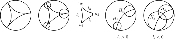
Figure 3: decorated ideal triangles and their edge lengths

It is known that for any $l_{1},l_{2},l_{3}\in\mathbb{R}$, there exists a unique decorated ideal triangle of edge lengths $l_{1},l_{2},l_{3}$. The relationship between the lengths $l_{i}$ and angles $a_{j}$’s is the following cosine law proved by Penner:

$$a_{i}=e^{\frac{1}{2}(l_{i}-l_{j}-l_{k})}=\frac{L_{i}}{L_{j}L_{k}},\quad\quad\ln(a_{i})+\ln(a_{j})=-l_{k},\quad\quad\{i,j,k\}=\{1,2,3\}.$$ (6)

Let $S$ be a closed connected surface and $V=\{v_{1},...,v_{n}\}\subset S$ and $\Sigma=S-V$. We assume $n\geq 1$ and $\chi(\Sigma)<0$. Following Penner, a decorated hyperbolic metric on $\Sigma$ is a complete finite area hyperbolic metric $d$ on $\Sigma$ together with a horoball $H_{i}$ centered at the i-th cusp at $v_{i}$ for each $i$. We can also parameterize it as $(d,w)$ where $w=(w_{1},...,w_{n})\in\mathbb{R}^{n}_{>0}$ with $w_{i}$ being the length of the horocycle $\partial H_{i}$. Two decorated hyperbolic metrics on $\Sigma$ are equivalent if there is an isometry $h$ between them so that $h$ is homotopic to the identity and $h$ preserves the horoballs. The space of all equivalence classes of decorated hyperbolic metrics on $\Sigma$ is defined to be the decorated Teichmüller space $T_{D}(\Sigma)$. If we use $T(\Sigma)$ to denote the usual Teichmüller space of complete hyperbolic metrics of finite area on $\Sigma$, then there is a natural homeomorphism from $T_{D}(\Sigma)$ to $T(\Sigma)\times\mathbb{R}^{n}_{>0}$ by sending $[(d,w)]$ to $([d],w)$. The projection $T_{D}(\Sigma)\to T(\Sigma)$ sending $[(d,w)]$ to $[d]$ records the underlying hyperbolic metric.

Now suppose $\mathcal{T}$ is a triangulation of $(S,V)$ with $E=E(\mathcal{T})$. Then Penner introduced a homeomorphism map $\Psi_{\mathcal{T}}:\mathbb{R}_{>0}^{E}\to T_{D}(\Sigma)$ called $\lambda$-length coordinate as follows. For each $x\in\mathbb{R}_{>0}^{E}$, i.e., $x:E\to\mathbb{R}_{>0}$, $\Psi_{\mathcal{T}}(x)$ is the equivalence class of the decorated hyperbolic metric $(d,w)$ on $\Sigma$ obtained as follows. If $t$ is a triangle in $\mathcal{T}$ with three edges $e_{i},e_{j},e_{k}$, one replaces $t$ by the decorated ideal triangle of edge lengths $2\ln x(e_{i}),2\ln x(e_{j})$ and $2\ln x(e_{k})$ and glues these decorated ideal triangles isometrically along the corresponding edges preserving decoration. One obtains a decorated hyperbolic metric $(d,w)$ on $\Sigma$. The horoballs are the gluing of the corresponding portions of horoballs associated to ideal triangles. In particular, $w_{i}$ is the sum of all angles of the decorated ideal triangles at $v_{i}$. Penner proved, using his Ptolemy identity, that $\Psi_{\mathcal{T}}^{-1}\Psi_{\mathcal{T}^{\prime}}$ is real analytic for any two triangulations $\mathcal{T}$ and $\mathcal{T}^{\prime}$. Here Ptolemy identity for decorated ideal quadrilaterals states that $AA^{\prime}+BB^{\prime}=CC^{\prime}$ where $A,A^{\prime},B,B^{\prime}$ are the $\lambda$-lengths of the edges of a quadrilateral and $C,C^{\prime}$ are the $\lambda$-lengths of the diagonals. See figure 4. In particular, $\{\Psi_{\mathcal{T}}|\mathcal{T}\}$ forms real analytic charts for $T_{D}(\Sigma)$.

The following lemma is well know. We omit the proof.

Lemma 3.1

Suppose $C$ is an embedded horocycle of length $w_{i}$ centered at a cusp in a complete hyperbolic surface and $C^{\prime}$ is another embedded horocycle of smaller length $w_{i}^{\prime}$ centered at the same cusp. Then the $w_{i}=w_{i}^{\prime}e^{t}$ where $t=d(C,C^{\prime})$ is the distance between $C$ and $C^{\prime}$.

By the lemma and definition, if $\Psi_{\mathcal{T}}(x)=[(d,w)]$ then for any $k>0$, $\Psi_{\mathcal{T}}(kx)=[(d,\frac{1}{k}w)]$. Thus, for any $(d,w)$, by choosing $k$ large, one may assume the associated horoballs are disjoint and embedded in $(d,w/k)$.

3.2 Delaunay triangulations

Given a decorated hyperbolic metric $(d,w)$ on $\Sigma$, there is a natural Delaunay triangulation $\mathcal{T}$ associated to $(d,w)$. The geometric definition of $\mathcal{T}$ goes as follows. First assume that the associated horoballs $H_{1}(w),...,H_{n}(w)$ are embedded and disjoint in $\Sigma$. Consider the Voronoi cell decomposition of the compact surface $X_{w}=\Sigma-\cup_{i=1}^{n}int(H_{i}(w))$ so that the 2-cell $R_{i}(w)$ associated to $v_{i}$ is $\{x\in X_{w}|d(x,\partial H_{i}(w))\leq d(x,\partial H_{j}(w)),\text{ all $j$}\}$. An orthogeodesic in $X_{w}$ is a geodesic from $\partial X_{w}$ to $\partial X_{w}$ perpendicular to $\partial X_{w}$. The dual of the Voronoi decomposition is a decomposition $\mathcal{C}(d,w)$ of $X$ by a collection of disjoint embedded orthogeodesics arcs $\{s^{\prime}\}$ constructed as follows. If $s\subset R_{i}(w)\cap R_{j}(w)$ is a geodesic segment, take a point $p\in S$ and consider the two shortest geodesics $b_{i}$ and $b_{j}$ in $R_{i}(w)$ and $R_{j}(w)$ respectively from $p$ to $\partial H_{i}(w)$ and $\partial H_{j}(w)$. The shortest orthogeodesic $s^{\prime}$ in $X_{w}$ homotopic to $b^{-1}_{i}*b_{j}$ is an arc in $\mathcal{D}(d)$ dual to $s$. A Delaunay triangulation of $X_{w}$ is a further decomposition of $\mathcal{C}(d,w)$ by decomposing all non-hexagonal 2-cells by orthogeodesic. Since each orthogeodesic extends to a complete geodesic from cusp to cusp, one obtains a Delaunay triangulation $\mathcal{T}(d,w)$ of the decorated metric $(d,w)$ on $\Sigma$ by extension. For a generic metric $(d,w)$, a Delaunay triangulation is the dual to the Voronoi decomposition. By the definition of Voronoi cells and lemma 3.1, Delaunay triangulations of $(d,w)$ and $(d,w/k)$ are the same when $k>1$. Due to this, for a general decorated metric $(d,w)$, we define a Delaunay triangulation of $(d,w)$ to be that of $(d,w/k)$ for $k$ large.

For a given triangulation $\mathcal{T}$ of $(S,V)$, let $D(\mathcal{T})$ be the set of all equivalence classes of decorated hyperbolic metrics $(d,w)$ in $T_{D}(\Sigma)$ so that $\mathcal{T}$ is isotopic to a Delaunay triangulation of $(d,w)$. Penner proved the following important theorem in [18]. Details on the real analytic diffeomorphism part of the decomposition can be found in [10].

Theorem 3.2

(Penner) The decorated Teichmüller space $T_{D}(\Sigma)$ has a real analytic cell decomposition by $\{D(\mathcal{T})|\mathcal{T}\}$ and

$$T_{D}(\Sigma)=\cup_{[\mathcal{T}]}D(\mathcal{T})$$

where the union is over all isotopy classes of triangulations. The decomposition is invariant under the action of the mapping class group.

3.3 Finite set of Delaunay triangulations

We thank B. Springborn for informing us the following result was known before and was a theorem of Akiyoshi [1]. However, our proof is different and short. For completeness, we present our proof in the appendix. The theorem holds for decorated finite volume hyperbolic manifolds of any dimension.

Theorem 3.3

(Akiyoshi) For any finite area complete hyperbolic metric $d$ on $\Sigma$, there are only finitely many isotopy classes of triangulations $\mathcal{T}$ so that $([d]\times\mathbb{R}_{>0}^{n})\cap D(\mathcal{T})\neq\emptyset$. In particular, there exist triangulations $\mathcal{T}_{1}$, …, $\mathcal{T}_{k}$ so that for any $w\in R_{>0}^{n}$, any Delaunay triangulation $(d,w)$ is isotopic to one of $\mathcal{T}_{i}$.

4 Euclidean polyhedral metrics and decorated hyperbolic metrics

The relationship between edge length coordinate of PL metrics with that of $\lambda$-length was first noticed in [4]. Fix a triangulation $\mathcal{T}$ of $(S,V)$, we have two coordinate maps $\Phi^{-1}_{\mathcal{T}}:P(\mathcal{T})\to\mathbb{R}^{E(\mathcal{T})}$ and $\Psi_{\mathcal{T}}:\mathbb{R}^{E(\mathcal{T})}\to T_{D}(S,V)$. Consider the injective map $A_{\mathcal{T}}:P(\mathcal{T})\to T_{D}(\Sigma)$ defined by $\Psi_{\mathcal{T}}\circ\Phi_{\mathcal{T}}^{-1}$.

Theorem 4.1

$A_{\mathcal{T}}|_{D_{pl}(\mathcal{T})}$ is a real analytic diffeomorphism from $D_{pl}(\mathcal{T})$ onto $D(\mathcal{T})$.

• To see that $A_{\mathcal{T}}$ maps $D_{pl}(\mathcal{T})$ bijectively onto $D(\mathcal{T})$, it suffices to show that $\Phi_{\mathcal{T}}^{-1}(D_{pl}(\mathcal{T}))=\Psi_{\mathcal{T}}^{-1}(D(\mathcal{T}))$.

  Recall that the characterization of a PL metric $d$ which is Delaunay in $\mathcal{T}$ in terms of $x=\Phi_{\mathcal{T}}^{-1}(d)$ is as follows. Take an edge $e\in E(\mathcal{T})$ and let $t$ and $t^{\prime}$ be the triangles adjacent to $e$ so that $e,e_{1},e_{2}$ are edges of $t$ and $e,e_{3},e_{4}$ are the edge of $t^{\prime}$. Suppose $\alpha,\alpha^{\prime}$ are the angles (measured in $d$) in $t$ and $t^{\prime}$ facing $e$. Then the Delaunay condition is equivalent to

  $$\alpha+\alpha^{\prime}\leq\pi,\quad\text{i.e.,}\quad\cos(\alpha)+\cos(\alpha^{\prime})\geq 0,\quad\text{for all edges $e\in E(\mathcal{T})$}.$$ (7)

  Suppose the length of $e$ (in $d$) is $x_{0}$ and the length of $e_{i}$ is $x_{i}$, $i=1,...,4$. By the cosine law, Delaunay condition (7) is the same as

  $$\frac{x_{1}^{2}+x_{2}^{2}-x_{0}^{2}}{2x_{1}x_{2}}+\frac{x_{3}^{2}+x_{4}^{2}-x_{0}^{2}}{2x_{3}x_{4}}\geq 0,\quad\text{for all edges $e\in E(\mathcal{T})$}.$$ (8)

  This shows that

  $$\Phi_{\mathcal{T}}^{-1}(D_{pl}(\mathcal{T}))=\{x\in\mathbb{R}_{>0}^{E}|\text{ (\ref{2.46}) holds for each edge $e$, and (\ref{2.47}) holds for each triangle}\}$$

  where

  $$x(e_{i})+x(e_{j})>x(e_{k}),\quad\text{ $e_{i},e_{j},e_{k}$ form edges of a triangle in $\mathcal{T}$}.$$ (9)

  Lemma 4.2

  Suppose $x:E(\mathcal{T})\to\mathbb{R}_{>0}$ so that (8) holds for all edges. Then (9) holds for all triangles.

  • Suppose otherwise, there exists $x\in\mathbb{R}_{>0}^{E}$ so that (8) holds but there is a triangle with edges $e_{i},e_{j},e_{k}$ so that

    $$x(e_{i})\geq x(e_{j})+x(e_{k}).$$ (10)

    In this case, we say $e_{i}$ is a ”bad” edge. Let $e$ be a ”bad” edge of the largest $x$ value, i.e., $x(e)=\max\{x(e_{i})|$ (10) holds}. Let $t$, $t^{\prime}$ be the triangles adjacent to $e$ and the edges of $t$ and $t^{\prime}$ be $\{e,e_{1},e_{2}\}$ and $\{e,e_{3},e_{4}\}$. Note that $t^{\prime}=t$ is allowed if $e$ is adjacent to one triangle. Let $x_{0}=x(e)$, $x_{i}=x(e_{i})$ for $i=1,2,3,4$. Without loss of generality we may assume that

    $$x_{1}+x_{2}\leq x_{0}.$$ (11)

    Since $e$ is a ”bad” edge of the largest $x$ value, we have $x_{3}<x_{0}+x_{4}$ and $x_{4}<x_{0}+x_{3}$, i.e.,

    $$|x_{3}-x_{4}|<x_{0}.$$ (12)

    On the other hand, inequality (8) holds for $x_{0},x_{1},...,x_{4}$, i.e.,

    $$\frac{x_{0}^{2}-x_{1}^{2}-x_{2}^{2}}{2x_{1}x_{2}}\leq\frac{x_{3}^{2}+x_{4}^{2}-x_{0}^{2}}{2x_{3}x_{4}}.$$ (13)

    Inequality (11) says the left-hand-side of (13) is at least 1 and inequality (12) says the right-hand-side of (13) is strictly less than 1. This is a contradiction. $\square$

The space $\Psi_{\mathcal{T}}^{-1}(D(\mathcal{T}))$ can be characterized as follows. Suppose the $\lambda$-length of $(d^{\prime},w)\in D(\mathcal{T})$ is $x=\Psi_{\mathcal{T}}^{-1}(d^{\prime},w)$. For each edge $e$ in $(S,\mathcal{T},d^{\prime})$, let $a,a^{\prime}$ be the two angles facing $e$ and $b,b^{\prime},c,c^{\prime}$ be the angles adjacent to the edge $e$. Then $(d^{\prime},w)$ is Delaunay in $\mathcal{T}$ if and only if for each edge $e\in E(\mathcal{T})$ (see [18] or [10]),

$$a+a^{\prime}\leq b+b^{\prime}+c+c^{\prime}.$$ (14)

Let $t$ and $t^{\prime}$ be the triangle adjacent to $e$ and $e,e_{1},e_{2}$ be edges of $t$ and $e,e_{3},e_{4}$ be the edges of $t^{\prime}$. Let the $\lambda$-length of $e$ be $x_{0}$ and the $\lambda$-length of $e_{i}$ be $x_{i}$. Then using the cosine law (6), one sees that (14) is equivalent to

$$\frac{x_{0}^{2}}{x_{1}x_{2}}+\frac{x_{0}^{2}}{x_{3}x_{4}}\leq\frac{x_{1}}{x_{2}}+\frac{x_{2}}{x_{1}}+\frac{x_{3}}{x_{4}}+\frac{x_{4}}{x_{3}},\quad\text{for each $e\in E(\mathcal{T})$}.$$ (15)

Inequality (15) is equivalent to

$$0\leq\frac{x_{1}^{2}+x_{2}^{2}-x_{0}^{2}}{2x_{1}x_{2}}+\frac{x_{3}^{2}+x_{4}^{2}-x_{0}^{2}}{2x_{3}x_{4}},\quad\text{for each $e\in E(\mathcal{T})$}.$$ (16)

Therefore,

$$\Psi_{\mathcal{T}}^{-1}(D(\mathcal{T}))=\{x\in\mathbb{R}_{>0}^{E}|\text{ (\ref{3.5}) holds at each edge $e\in E(\mathcal{T})$}\}.$$

However, inequality (16) is the same as (8). This shows $\Phi_{\mathcal{T}}^{-1}(D_{pl}(\mathcal{T}))\subset\Psi_{\mathcal{T}}^{-1}(D(\mathcal{T}))$. On the other hand, lemma 4.2 implies that $\Phi_{\mathcal{T}}^{-1}(D_{pl}(\mathcal{T}))=\Psi_{\mathcal{T}}^{-1}(D(\mathcal{T}))$.

Finally, since both $\Phi_{\mathcal{T}}$ and $\Psi_{\mathcal{T}}$ are real analytic diffeomorphisms and $A_{\mathcal{T}}=\Psi_{\mathcal{T}}\circ\Phi_{\mathcal{T}}^{-1}$ and $A^{-1}_{\mathcal{T}}=\Phi_{\mathcal{T}}\circ\Psi^{-1}_{\mathcal{T}}$, we see that $A_{\mathcal{T}}$ is a real analytic diffeomorphism. $\square$

4.1 Globally defined map, diagonal switch and Ptolemy relation

Theorem 4.3

Suppose $\mathcal{T}$ and $\mathcal{T}^{\prime}$ are two triangulations of $(S,V)$ so that $D_{pl}(\mathcal{T})\cap D_{pl}(\mathcal{T}^{\prime})\neq\emptyset$. Then

$$A_{\mathcal{T}}|_{D_{pl}(\mathcal{T})\cap D_{pl}(\mathcal{T}^{\prime})}=A_{\mathcal{T}^{\prime}}|_{D_{pl}(\mathcal{T})\cap D_{pl}(\mathcal{T}^{\prime})}.$$ (17)

In particular, the gluing of these $\mathbf{A}_{\mathcal{T}}|_{D_{pl}(\mathcal{T})}$ mappings produces a homeomorphism $\mathbf{A}=\cup_{\mathcal{T}}\mathbf{A}_{\mathcal{T}}|_{D_{pl}(\mathcal{T})}:T_{pl}(S,V)\to T_{D}(S-V)$ such that $A([d])$ and $A([d^{\prime}])$ have the same underlying hyperbolic structure if and only if $d$ and $d^{\prime}$ are discrete conformal.

• Suppose $[d]\in D_{pl}(\mathcal{T})\cap D_{pl}(\mathcal{T}^{\prime})$, i.e., $\mathcal{T}$ and $\mathcal{T}^{\prime}$ are both Delaunay in the PL metric $d$. Then it is known that there exists a sequence of triangulations $\mathcal{T}_{1}=\mathcal{T},\mathcal{T}_{2},...,T_{k}=\mathcal{T}^{\prime}$ on $(S,V)$ so that each $\mathcal{T}_{i}$ is Delaunay in $d$ and $\mathcal{T}_{i+1}$ is obtained from $\mathcal{T}_{i}$ by a diagonal switch. In particular, $A_{\mathcal{T}}([d])=A_{\mathcal{T}^{\prime}}([d])$ follows from $A_{\mathcal{T}_{i}}([d])=A_{\mathcal{T}_{i+1}}([d])$ for $i=1,2,...,k-1$. Thus, it suffices to show $A_{\mathcal{T}}([d])=A_{\mathcal{T}^{\prime}}([d])$ when $\mathcal{T}^{\prime}$ is obtained from $\mathcal{T}$ by a diagonal switch along an edge $e$. In this case the transition functions $\Phi_{\mathcal{T}}^{-1}\Phi_{\mathcal{T}^{\prime}}$ and $\Psi_{\mathcal{T}}^{-1}\Psi_{\mathcal{T}^{\prime}}$ are the diagonal switch formulas. Penner proved an amazing result that the $\lambda$-lengths satisfy the Ptolemy identity for decorated ideal quadrilaterals. See [18] and figure 4. This result, translated into the language of length coordinates, says that $\Phi_{\mathcal{T}}^{-1}\Phi_{\mathcal{T}^{\prime}}(x)=\Psi_{\mathcal{T}}^{-1}\Psi_{\mathcal{T}^{\prime}}(x)$ for $x\in\Phi^{-1}_{\mathcal{T}}(D_{pl}(\mathcal{T})\cap D_{pl}(\mathcal{T}^{\prime}))$. This is the same as (17). Taking the inverse, we obtain

  $$A_{\mathcal{T}}^{-1}|_{D(\mathcal{T})\cap D(\mathcal{T}^{\prime})}=A_{\mathcal{T}^{\prime}}^{-1}|_{D(\mathcal{T})\cap D(\mathcal{T}^{\prime})}.$$ (18)

  Lemma 4.4

  (a) $D_{pl}(\mathcal{T})\cap D_{pl}(\mathcal{T}^{\prime})\neq\emptyset$ if and only if $D(\mathcal{T})\cap D(\mathcal{T}^{\prime})\neq\emptyset$.

  (b) The gluing map $\mathbf{A}=\cup_{\mathcal{T}}\mathbf{A}_{\mathcal{T}}|_{D_{pl}(\mathcal{T})}:T_{pl}\to T_{D}$ is a homeomorphism invariant under the action of the mapping class group.

  • By (17) and (18), the maps $\mathbf{A}=\cup_{\mathcal{T}}\mathbf{A}_{\mathcal{T}}|_{D_{pl}(\mathcal{T})}:T_{pl}\to T_{D}$ and $\mathbf{B}=\cup_{\mathcal{T}}\mathbf{A}^{-1}_{\mathcal{T}}|_{D(\mathcal{T})}:T_{D}\to T_{pl}$ are well defined and continuous. Since $\mathbf{A}(D_{pl}(\mathcal{T})\cap D_{pl}(\mathcal{T}^{\prime}))\subset D(\mathcal{T})\cap D(\mathcal{T}^{\prime})$ and $\mathbf{B}(D(\mathcal{T})\cap D(\mathcal{T}^{\prime}))\subset D_{pl}(\mathcal{T})\cap D_{pl}(\mathcal{T}^{\prime})$, part (a) follows. To see part (b), since $T_{D}=\cup_{\mathcal{T}}D(\mathcal{T})$, the map $\mathbf{A}$ is onto. To see $\mathbf{A}$ is injective, suppose $x_{1}\in D_{pl}(\mathcal{T}_{1}),x_{2}\in D_{pl}(\mathcal{T}_{2})$ so that $\mathbf{A}(x_{1})=\mathbf{A}(x_{2})\in D(\mathcal{T}_{1})\cap D(\mathcal{T}_{2})$. Apply (18) to $\mathbf{A}^{-1}_{\mathcal{T}_{1}}|,\mathbf{A}^{-1}_{\mathcal{T}_{2}}|$ on the set $D(\mathcal{T}_{1})\cap D(\mathcal{T}_{2})$ at the point $A(x_{1})$, we conclude that $x_{1}=x_{2}$. This shows that $\mathbf{A}$ is a bijection with inverse $\mathbf{B}$. Since both $\mathbf{A}$ and $\mathbf{B}$ are continuous, $\mathbf{A}$ is a homeomorphism. $\square$

Now if $d$ and $d^{\prime}$ are two discrete conformally equivalent PL metrics, then $\mathbf{A}([d])$ and $\mathbf{A}([d^{\prime}])$ are of the form $(p,w)$ and $(p,w^{\prime})$ due to the definition of $\Psi^{-1}_{\mathcal{T}}\Phi_{\mathcal{T}}$. On the other hand, if two PL metrics $d,d^{\prime}$ satisfy that $\mathbf{A}([d])$ and $\mathbf{A}([d^{\prime}])$ are of the form $(p,w)$ and $(p,w^{\prime})$, consider a generic smooth path $\gamma(t)=(p,w(t)),t\in[0,1]$, in $T_{D}(\Sigma)$ from $(p,w)$ to $(p,w^{\prime})$ so that $\gamma(t)$ intersects the cells $D(\mathcal{T})$’s transversely. This implies that $\gamma$ passes through a finite set of cells $D(\mathcal{T}_{i})$ and $\mathcal{T}_{j}$ and $\mathcal{T}_{j+1}$ are related by a diagonal switch. Let $t_{0}=0<...<t_{m}=1$ be a partition of $[0,1]$ so that $\gamma([t_{i},t_{i+1}])\subset D(\mathcal{T}_{i})$. Say $d_{i}$ is the PL metric so that $\mathbf{A}([d_{i}])=\gamma(t_{i})\in D(\mathcal{T}_{i})\cap D(\mathcal{T}_{i+1})$, $d_{1}=d$ and $d_{m}=d^{\prime}$. Then by definition, the sequences $\{d_{1},...,d_{m}\}$ and the associated Delaunay triangulations $\{\mathcal{T}_{1},...,T_{m}\}$ satisfy the definition of discrete conformality for $d,d^{\prime}$. $\square$

Theorem 4.5

The homeomorphism $\mathbf{A}:T_{pl}(S,V)\to T_{D}(S-V)$ is a $C^{1}$ diffeomorphism.

• It suffices to show that for a point $[d]\in D_{pl}(\mathcal{T})\cap\mathcal{D}_{pl}(\mathcal{T}^{\prime})$, the derivatives $DA_{\mathcal{T}}[d])$ and $DA_{\mathcal{T}^{\prime}}([d])$ are the same. Since both $\mathcal{T}$ and $\mathcal{T}^{\prime}$ are Delaunay in $d$ and are related by a sequence of Delaunay triangulations (in $d$) $\mathcal{T}_{1}=\mathcal{T},\mathcal{T}_{2},...,\mathcal{T}_{k}=\mathcal{T}^{\prime}$, $DA_{\mathcal{T}}([d])=DA_{\mathcal{T}^{\prime}}([d])$ follows from $DA_{\mathcal{T}_{i}}([d])=DA_{\mathcal{T}_{i+1}}([d])$ for $i=1,2,...,k-1$. Therefore, it suffices to show $DA_{\mathcal{T}}([d])=DA_{\mathcal{T}^{\prime}}([d])$ when $\mathcal{T}$ and $\mathcal{T}^{\prime}$ are related by a diagonal switch at an edge $e$. In the coordinates $\Phi_{\mathcal{T}}$ and $\Psi_{\mathcal{T}}$, the fact that $DA_{\mathcal{T}}([d])=DA_{\mathcal{T}^{\prime}}([d])$ is equivalent to the following smoothness question on the diagonal lengths.

  Lemma 4.6

  Suppose $Q$ is a convex Euclidean quadrilateral whose four edges are of lengths $x,y,z,w$ and the length of a diagonal is $a$. See figure 4. Suppose $A(x,y,z,w,a)$ is the length of the other diagonal and $B(x,y,z,w,a)=\frac{xz+yw}{a}$. If a point $(x,y,z,w,a)$ satisfies $A(x,y,z,w,a)=B(x,y,z,w,a)$, i.e., $Q$ is inscribed in a circle, then $DA(x,y,z,w,a)=DB(x,y,z,w,a)$ where $DA$ is the derivative of $A$.

Figure 4: Euclidean and hyperbolic Ptolemy

• The roles of $x,y,z,w$ are symmetric with respect to $a$. Hence it suffices to show that $\frac{\partial A}{\partial a}=\frac{\partial B}{\partial a}$ and $\frac{\partial A}{\partial x}=\frac{\partial B}{\partial x}$ at these points. First, we have $\frac{\partial B}{\partial x}=\frac{z}{a}$ and $\frac{\partial B}{\partial a}=-\frac{B}{a}$.

  Now let $\alpha,\alpha^{\prime},\beta,\beta^{\prime}$ be the angles formed by the pairs of edges $\{y,a\}$, $\{a,x\}$, $\{a,z\}$ and $\{a,w\}$. By the cosine law, we have

  $$A^{2}=y^{2}+z^{2}-2yz\cos(\alpha+\beta).$$

  Take partial $x$ derivative of it. We obtain

  $$2A\frac{\partial A}{\partial x}=2yz\sin(\alpha+\beta)\frac{\partial\alpha}{\partial x}.$$

  But it is well known (see for instance [17]) that in the triangle of lengths $x,y,a$,

  $$\frac{\partial\alpha}{\partial x}=\frac{x}{ay\sin(\alpha)}.$$ (19)

  Therefore,

  $$\frac{\partial A}{\partial x}=\frac{xz\sin(\alpha+\beta)}{aA\sin(\alpha)}.$$

  Now at the point where $A(x,y,z,w,a)=B(x,y,z,w,a)$, the quadrilateral is inscribed to the circle. Therefore, $\frac{\sin(\alpha+\beta)}{\sin(\alpha)}=\frac{A}{x}$. By putting these together, we see that $\frac{\partial A}{\partial x}=\frac{xzA}{aAx}=\frac{z}{a}=\frac{\partial B}{\partial x}$.

  Next, we calculate $\frac{\partial A}{\partial a}$. By the formula above, we obtain $2A\frac{\partial A}{\partial a}=2yz\sin(\alpha+\beta)(\frac{\partial\alpha}{\partial a}+\frac{\partial\beta}{\partial a}).$ Now by the derivative cosine law ([8]), we have $\frac{\partial\alpha}{\partial a}=-\frac{\partial\alpha}{\partial x}\cos(\alpha^{\prime})$ which in turn is $-\frac{x\cos(\alpha^{\prime})}{ay\sin(\alpha)}$ by (19). Similarly, we have $\frac{\partial\beta}{\partial a}=-\frac{w\cos(\beta^{\prime})}{az\sin(\beta)}$. Putting these together, we obtain,

  $$\frac{\partial A}{\partial a}=-\frac{yz\sin(\alpha+\beta)}{aA}(\frac{x\cos(\alpha^{\prime})}{y\sin(\alpha)}+\frac{w\cos(\beta^{\prime})}{z\sin(\beta)}).$$

  Now since $A=B$, the quadrilateral is inscribed in a circle, therefore, $\frac{\sin(\alpha+\beta)}{\sin(\alpha)}=\frac{A}{x}$ and $\frac{\sin(\alpha+\beta)}{\sin(\beta)}=\frac{A}{w}.$ Therefore, $\frac{\partial A}{\partial a}=-\frac{1}{a}(z\cos(\alpha^{\prime})+y\cos(\beta^{\prime}))=-\frac{A}{a}=-\frac{B}{a}=\frac{\partial B}{\partial a}$ where the identity $A=z\cos(\alpha^{\prime})+y\cos(\beta^{\prime})$ comes from the triangle of lengths $y,z,A$ and the fact that $Q$ is inscribed in a circle. $\square$

5 A proof of the main theorem

Using the map $\mathbf{A}:T_{pl}(S,V)\to T_{D}(\Sigma)$, we see that for a given PL metric $d$ on $(S,V)$, the set $\{[d^{\prime}]|\text{$d^{\prime}$ is discrete}$ $\text{ conformal to $d$}\}$ is $C^{1}$-diffeomorphic to $\{p\}\times\mathbb{R}_{>0}^{n}\subset T_{D}(S-V)$ for some $p\in T(\Sigma)$. Therefore, the discrete uniformization theorem is equivalent to a statement about the discrete curvature map defined on $\{p\}\times\mathbb{R}_{>0}^{n}\subset T_{D}(S-V)$. Let us make a change of variables from $w=(w_{1},...,w_{n})\in R_{>0}^{n}$ to $u=(u_{1},...,u_{n})\in\mathbb{R}^{n}$ where $u_{i}=\ln(w_{i})$. We write $w=w(u)$. For a given $p\in T(\Sigma)$, define the curvature map $\mathbf{F}:\mathbb{R}^{n}\to(-\infty,2\pi)^{n}$ by

$$\mathbf{F}(u)=K_{\mathbf{A}^{-1}(p,w(u))}$$ (20)

where $K_{d}$ is the discrete curvature. The map satisfies the property that $\mathbf{F}(u+k(1,1,...,1))=\mathbf{F}(u)$ and $\mathbf{F}(u)$ lies in the plane $GB=\{x\in\mathbb{R}^{n}|\sum_{i=1}^{n}x_{i}=2\pi\chi(S)\}$ defined by the Gauss-Bonnet identity. Let $P=\{u\in\mathbb{R}^{n}|\sum_{i=1}^{n}u_{i}=0\}$ and $Q=GB\cap(-\infty,2\pi)^{n}$. Then the restriction $F:=\mathbf{F}|_{P}:P\to Q$. The discrete uniformization theorem is equivalent to say that $F:P\to Q$ is a bijection. We will show that $F$ is a homeomorphism in this section.

We will prove that $F:P\to Q$ is injective in §5.2 using a variational principle developed in [16]. Assuming injectivity, we show that $F:P\to Q$ is onto in §5.1.

5.1 The map $F$ is onto

Assuming that $F$ is injective, we prove $F$ is onto in this section. Since both $P$ and $Q$ are connected manifolds of dimension $n-1$ and $F$ is injective and continuous, it follows that $F(P)$ is open in $Q$. To show that $F$ is onto, it suffices to prove that $F(P)$ is closed in $Q$.

To this end, take a sequence $\{u^{(m)}\}$ in $P$ which leaves every compact set in $P$. We will show that $\{F(u^{(m)})\}$ leaves each compact set in $Q$. By taking subsequences, we may assume that for each index $i=1,2,...,n$, the limit $\lim_{m}u^{(m)}_{i}=t_{i}$ exists in $[-\infty,\infty]$. Furthermore, since the space $\{p\}\times P$ is in the union of a finite set of Delaunay cells $D(\mathcal{T})$, we may assume, after taking another subsequence, that the corresponding PL metrics $d_{m}=\mathbf{A}^{-1}(p,w(u^{(m)}))$ are Delaunay in one triangulation $\mathcal{T}$. We will do our calculation in the length coordinate $\Phi_{\mathcal{T}}$ below.

Due to the normalization that $\sum_{i}u^{(m)}_{i}=0$ and $u^{(m)}$ does not converge to any vector in $P$, there exists $t_{i}=\infty$ and $t_{j}=-\infty$. Let us label vertices $v\in V$ by black and white as follows. The vertex $v_{i}$ is black if and only if $t_{i}=-\infty$ and all other vertices are white.

Lemma 5.1

(a) There does not exist a triangle $\tau\in\mathcal{T}$ with exactly two white vertices.

(b) If $\Delta v_{1}v_{2}v_{3}$ is a triangle in $\mathcal{T}$ with exactly one white vertex at $v_{1}$, then the inner angle of the triangle at $v_{1}$ converges to $0$ as $m\to\infty$ in the metrics $d_{m}$.

• To see (a), suppose otherwise, using the $\Phi_{\mathcal{T}}$ length coordinate, we see the given assumption is equivalent to following. There exists a Euclidean triangle of lengths $a_{i}e^{u^{(m)}_{j}+u^{(m)}_{k}}$, $\{i,j,k\}=\{1,2,3\}$, where $\lim_{m}u^{(m)}_{i}>-\infty$ for $i=2,3$ and $\lim_{m}u^{(m)}_{1}=-\infty$. By the triangle inequality, we have

  $$a_{2}e^{u^{(m)}_{1}+u^{(m)}_{3}}+a_{3}e^{u^{(m)}_{1}+u^{(m)}_{2}}>a_{1}e^{u^{(m)}_{2}+u^{(m)}_{3}}$$

  This is the same as

  $$a_{2}e^{-u^{(m)}_{2}}+a_{3}e^{-u^{(m)}_{3}}>a_{1}e^{-u^{(m)}_{1}}.$$

  However, by the assumption, the right-hand-side tends to $\infty$ and the left-hand-side is bounded. The contradiction shows that (a) holds.

  To see (b), we use the same notation as in the proof of (a). Let the length $l^{(m)}_{i}$ of the edge $v_{j}v_{k}$ in metric $d_{m}$ be $a_{i}e^{u^{(m)}_{j}+u^{(m)}_{k}}$, $\{i,j,k\}=\{1,2,3\}$. Let $\alpha_{i}:=\alpha_{i}(m)$ be the inner angle at $v_{i}$. Note that the triangle is similar to the triangle of lengths $a_{i}e^{-u^{(m)}_{i}}$ and $\lim_{m}a_{i}e^{-u^{(m)}_{i}}$ is $\infty$ when $i=2,3$ and is finite for $i=1$. Therefore, the angle $\alpha_{1}$ tends to 0. $\square$

We now finish the proof of $F(P)=Q$ as follows. Since the surface $S$ is connected, there exists an edge $e$ whose end points $v,v_{1}$ have different colors. Assume $v$ is white and $v_{1}$ is black. Let $v_{1},...,v_{k}$ be the set of all vertices adjacent to $v$ so that $v,v_{i},v_{i+1}$ form vertices of a triangle and let $v_{k+1}=v_{1}$. Now apply above lemma to triangle $\Delta vv_{1}v_{2}$ with $v$ white and $v_{1}$ black, we conclude that $v_{2}$ must be black. Repeating this to $\Delta vv_{2}v_{3}$ with $v$ white and $v_{2}$ black, we conclude $v_{3}$ is black. Inductively, we conclude that all $v_{i}$’s, for $i=1,2,...,k$, are black. By part (b) of the above lemma, we conclude that the curvature of $d_{m}$ at $v$ tends to $2\pi$. This shows that $F(u^{(m)})$ tends to infinity of $Q$. Therefore $F(P)=Q$.

5.2 Injectivity of $F$

The proof uses a variational principle developed in [16]. Recall that the map $\mathbf{F}:\mathbb{R}^{n}\to\mathbb{R}^{n}$ is the discrete curvature map $K_{\mathbf{A}^{-1}(p,w(u))}$ given by (20). Since $\mathbf{A}$ is a $C^{1}$ diffeomorphism and the discrete curvature $K:\mathcal{T}_{pl}(S,V)\to\mathbb{R}^{V}$ is real analytic, hence the map $\mathbf{F}$ is $C^{1}$ smooth. Let $\mathcal{T}_{i}$, $i=1,...,k$, be the set of all triangulations so that $(\{p\}\times\mathbb{R}^{n})\cap D(\mathcal{T}_{i})\neq\emptyset$ and $\{p\}\times\mathbb{R}^{n}\subset\cup_{i=1}^{k}D(\mathcal{T}_{i})$.

Lemma 5.2

Let $\phi:\mathbb{R}^{n}\to\{p\}\times\mathbb{R}^{n}$ be $\phi(x)=(p,x)$ and $U_{i}=\phi^{-1}((\{p\}\times\mathbb{R}^{n})\cap D(\mathcal{T}_{i}))\subset\mathbb{R}^{n}$ and $J=\{i|$ $int(U_{i})\neq\emptyset$}. Then $\mathbb{R}^{n}=\cup_{i\in J}U_{i}$ and $U_{i}$ is real analytic diffeomorphic to a convex polytope in $\mathbb{R}^{n}$.

• By definition, both $\{p\}\times\mathbb{R}^{n}$ and $D(\mathcal{T}_{i})$ are closed and semi algebraic in $T_{D}(\Sigma)$. Therefore $U_{i}$ is closed and semi-algebraic. Now by definition, $X:=\cup_{i\in J}U_{i}$ is a closed subset of $\mathbb{R}^{n}$ since $U_{i}$ is closed. If $X\neq\mathbb{R}^{n}$, then the complement $\mathbb{R}^{n}-X$ is a non-empty open set which is a finite union of real algebraic sets of dimension less than $n$. This is impossible.

  Finally, we will show that for any triangulation $\mathcal{T}$ of $(S,V)$ and $p\in T(\Sigma)$, the intersection $U=\phi^{-1}((\{p\}\times R^{n})\cap D(\mathcal{T}))$ is real analytically diffeomorphic to a convex polytope in a Euclidean space. In fact $\Psi_{\mathcal{T}}^{-1}(U)\subset\mathbb{R}^{E(\mathcal{T})}$ is real analytically diffeomorphic to a convex polytope. To this end, let $b=\Psi_{\mathcal{T}}^{-1}(p,(1,1,....,1))$. By definition, $\Psi_{\mathcal{T}}^{-1}(U)$ is give by

  $$\{x\in\mathbb{R}^{E(\mathcal{T})}_{>0}|\exists\lambda\in\mathbb{R}_{>0}^{V},x(e)=b(e)\lambda(v_{1})\lambda(v_{2}),\partial e=\{v_{1},v_{2}\},\text{Delaunay condition (\ref{4}) holds for $x$}\}.$$

  We claim that the Delaunay condition (15) consists of linear inequalities in the variable $\delta:V\to\mathbb{R}_{>0}$ where $\delta(v)=\lambda(v)^{-2}$. Indeed, suppose the two triangles adjacent to the edge $e=(v_{1},v_{2})$ have vertices $v_{1},v_{2},v_{3}$ and $v_{1},v_{2},v_{4}$ as shown in figure 2. Let $x_{ij}$ (respectively $b_{ij}$) be the value of $x$ (respectively $b$) at the edge joining $v_{i},v_{j}$, and $\lambda_{i}=\lambda(v_{i})$. By definition, $x_{ij}=b_{ij}\lambda_{i}\lambda_{j}$. The Delaunay condition (15) at the edge $e=(v_{1}v_{2})$ says that

  $$\frac{x_{12}^{2}}{x_{31}x_{32}}+\frac{x_{12}^{2}}{x_{41}x_{42}}\leq\frac{x_{31}}{x_{32}}+\frac{x_{32}}{x_{31}}+\frac{x_{41}}{x_{42}}+\frac{x_{42}}{x_{41}}$$ (21)

  It is the same as, using $x_{ij}=b_{ij}\lambda_{i}\lambda_{j}$,

  $$c_{3}\frac{\lambda_{1}\lambda_{2}}{\lambda_{3}^{2}}+c_{4}\frac{\lambda_{1}\lambda_{2}}{\lambda_{4}^{2}}\leq c_{1}\frac{\lambda_{2}}{\lambda_{1}}+c_{2}\frac{\lambda_{1}}{\lambda_{2}},$$

  where $c_{i}$ is some constant depending only on $b_{jk}$’s. Dividing above inequality by $\lambda_{1}\lambda_{2}$ and using $\delta_{i}=\lambda_{i}^{-2}$, we obtain

  $$c_{3}\delta_{3}+c_{4}\delta_{4}\leq c_{1}\delta_{1}+c_{2}\delta_{2}$$ (22)

  at each edge $e\in E(\mathcal{T})$. This shows for $b$ fixed, the set of all possible values of $\delta$ form a convex polytope $Q$ defined by (22) at all edges and $\delta(v)>0$ at all $v\in V$. On the other hand, by definition, the map from $Q$ to $\Psi_{\mathcal{T}}^{-1}(U)$ sending $\delta$ to $x=x(\delta)$ given by $x(vv^{\prime})=\frac{b(vv^{\prime})}{\sqrt{\delta(v)\delta(v^{\prime})}}$ is a real analytic diffeomorphism. Thus the result follows. $\square$

Write $\mathbf{F}=(F_{1},...,F_{n})$ which is $C^{1}$ smooth. By theorems 1.2 and 2.1 of [16], one sees that (a) $F_{j}|_{U_{h}}$ is real analytic so that $\frac{\partial F_{i}}{\partial u_{j}}=\frac{\partial F_{j}}{\partial u_{i}}$ in $U_{h}$ for all $h\in J$ and (b) the Hessian matrix $[\frac{\partial F_{i}}{\partial u_{j}}]$ is positive semi-definition on each $U_{h}$ so that its kernel consists of vectors $\lambda(1,1,...,1)$. Therefore, the 1-form $\eta=\sum_{i}F_{i}(u)du_{i}$ is a $C^{1}$ smooth 1-form on $\mathbb{R}^{n}$ so that $d\eta=0$ on each $U_{h},h\in J$. This implies that $d\eta=0$ in $\mathbb{R}^{n}$. Hence the integral $W(u)=\int_{0}^{u}\eta$ is a well defined $C^{2}$ smooth function on $\mathbb{R}^{n}$ so that its Hessian matrix is positive semi-definition. Therefore, $W$ is convex in $\mathbb{R}^{n}$ so that its gradient $\bigtriangledown W=\mathbf{F}$. Furthermore, since the kernel of the Hessian of $W$ consists of diagonal vectors $\lambda(1,1,...,1)$ at each point in $U_{h},h\in J$ and $\mathbb{R}^{n}=\cup_{h\in J}U_{h}$, the Hessian of the function $W|_{P}$ is positive definite. Hence $W|_{P}$ is strictly convex. Now we use the following well known lemma,

Lemma 5.3

If $W:\Omega\to\mathbb{R}$ is a $C^{1}$-smooth strictly convex function on an open convex set $\Omega\subset\mathbb{R}^{m}$, then its gradient $\bigtriangledown W:\Omega\to\mathbb{R}^{m}$ is an embedding.

Apply the lemma to $W|_{P}$ and use $\bigtriangledown(W|_{P})=F$, we conclude that $F:P\to Q$ is injective.

The discrete Yamabe flow with surgery is the gradient flow of the strictly convex function $W(u)-\sum_{i=1}^{n}K^{*}_{i}u_{i}$ which has a unique minimal point in $P$. In the formal notation, the flow takes the form $\frac{du_{i}(t)}{dt}=K_{i}-K^{*}_{i}$ and $u(0)=0$. The exponential convergence of the flow was established in theorem 1.4 of [16].

6 A Conjecture

We conjecture that the number of surgery operations used in the discrete Yamabe flow to find the target PL metric is finite, i.e., along the integral curve of the gradient flow of the function $W(u)-\sum_{i=1}^{n}K^{*}_{i}u_{i}$, only finitely many diagonal switches occur. This is supported by our numerical experiments.

There should be a related theory of discrete conformal maps associated to the discrete Riemann surfaces introduced in this paper. See [22] for the corresponding discrete conformal maps for circle packing.

David Gu, Department of Computer Science, Stony Brook University, New York 11794, USA.
Email: gu$@$cs.stonybrook.edu.

Feng Luo, Department of Mathematics, Rutgers University, New Brunswick, NJ 08854, USA.
Email: fluo$@$math.rutgers.edu

Jian Sun, Mathematical Sciences Center, Tsinghua University, Beijing 100084, China.
Email: jsun$@$math.tsinghua.edu.cn.

Tianqi Wu, Mathematical Sciences Center, Tsinghua University, Beijing 100084, China.
Email: mike890505$@$gmail.com.

Appendix: A proof of Akiyoshi’s theorem

For completeness, we present our proof in this appendix. The theorem and the proof hold for decorated finite volume hyperbolic manifolds of any dimension. We state the 2-dimensional case for simplicity.

Theorem 6.1

(Akiyoshi [1]) For a finite area complete hyperbolic metric $d$ on $\Sigma$, there exist triangulations $\mathcal{T}_{1}$, …, $\mathcal{T}_{k}$ so that for any $w\in R_{>0}^{n}$, any Delaunay triangulation of $(d,w)$ is isotopic $\mathcal{T}_{i}$, $i\in\{1,2,...,k\}$.

• We begin by study the shortest geodesics in a complete finite area hyperbolic surface $(\Sigma,d)$. Recall the Shimizu lemma [3] which implies that if $w\in(0,1)^{n}$, then the associated horoballs $H_{i}(w)$ in the decorated metric $(d,w)$ are embedded and pairwise disjoint. Let us assume without loss of generality that $w\in(0,1)^{n}$. A geodesic $\alpha$ from cusp $v_{i}$ to $v_{j}$ in $(\Sigma,d)$ is called a shortest geodesic from $v_{i}$ to $v_{j}$ if there exists a $w\in(0,1)^{n}$ so that $\alpha\cap X_{w}$ is a shortest path among all homotopically non-trivial paths in $X_{w}$ joining $\partial H_{i}(w)$ to $\partial H_{j}(w)$. The shortest property implies that $\alpha\cap X_{w}$ is an orthogeodesic. Furthermore, by lemma 3.1, if $\alpha$ is a shortest geodesic, then for any $w^{\prime}\in(0,1)^{n}$, $\alpha\cap X_{w^{\prime}}$ is again a shortest geodesic in $X_{w^{\prime}}$ from $\partial H_{i}(w^{\prime})$ to $\partial H_{j}(w^{\prime})$, i.e., being a shortest geodesic from $v_{i}$ to $v_{j}$ is independent of the choice of decorations. Indeed, for any geodesic $\beta$ from cusp $v_{i}$ to $v_{j}$, we have

  $$l(\beta\cap X_{w^{\prime}})=l(\beta\cap X_{w})-\ln(w_{i}^{\prime})-\ln(w_{j}^{\prime})+\ln(w_{i})+\ln(w_{j})$$ (23)

  Lemma 6.2

  Suppose $(\Sigma,d)$ is a finite area complete hyperbolic surface. Then

  (a) there are only finitely many shortest geodesics from $v_{i}$ to $v_{j}$.

  (b) there is $\delta_{ij}=\delta_{ij}(\Sigma,d)>0$ so that if $\alpha$ is a shortest geodesic from $v_{i}$ to $v_{j}$ and $\beta$ is another geodesic from $v_{i}$ to $v_{j}$ with $|l(\beta\cap X_{w})-l(\alpha\cap X_{w})|\leq\delta_{ij}$, then $\beta$ is a shortest geodesic.

  (c) given $v_{i}$, if $\alpha$ is a shortest orthogeodesic geodesics among all orthogeodesics in $X_{w}$ from $\partial H_{i}$ to $\partial X_{w}$, then $\alpha^{*}$, the complete geodesic containing $\alpha$, is an edge of the decorated metric $(d,w)$ and the mid-point of $\alpha$ is in $R_{j}(w)$.

  • The first part follows from the simple fact that on any compact surface $X_{w}$, for any constant $C$, there are only finitely many orthogeodesics of length at most $C$. Part (b) follows from (a) and equality (23). Part (c) follows from the definition of Voronoi cells and its dual. Note that in general, if $\beta$ is a shortest orthogeodesic in $X_{w}$ between $\partial H_{i}(w)$ and $\partial H_{j}(w)$, $\beta^{*}$ may not be an edge in any Delaunay triangulation of $(d,w)$. $\square$

Now we prove the theorem by contradiction. Suppose otherwise, there exists a sequence of decorated metrics $(d,w^{(m)})$ where $w^{(m)}=(w^{(m)}_{1},...,w^{(m)}_{n})\in\mathbb{R}^{n}$ so that the associated Delaunay triangulations $\mathcal{T}_{m}=\mathcal{T}(d,w^{(m)})$ are pairwise distinct in $(\Sigma,d)$. After normalizing $w^{(m)}$ by scaling, relabel the vertices $v_{1},...,v_{n}$ and taking subsequences, we may assume

(i) $w^{(m)}_{1}=\max\{w^{(m)}_{i}|i=1,2,...,n\}=1/2$;

(ii) for each $i=1,2,...,n$, the limit $\lim_{m}w^{(m)}_{i}=t_{i}\in[0,1/2]$ exists;

(iii) $t_{1},...,t_{k}>0$ and $t_{k+1}=...=t_{n}=0$.

For simplicity, we use $E_{ij}(\mathcal{T})$ to denote the subset of all edges of $\mathcal{T}$ joining $v_{i}$ to $v_{j}$. We will derive a contradiction by showing that $\cup_{m}E_{ij}(\mathcal{T}_{m})$ is a finite set.

Lemma 6.3

There exists a constant $C>0$ so that for all $i,j\leq k$, and all $e\in E_{ij}(\mathcal{T}_{m})$, the length

$$l(e\cap X_{w^{(m)}})\leq C.$$

In particular, $\cup_{m}E_{ij}(\mathcal{T}_{m})$ is a finite set.

• For any $\delta\in(0,1/2)$, let $u^{(m)}(\delta)=(w^{(m)}_{1},...,w^{(m)}_{k},\delta,...,\delta)\in\mathbb{R}^{n}$. Fix a $\delta$, since $\lim_{m}w^{(m)}_{j}=0$ for $j>k$, for $m$ large, each point $x\in X_{u^{(m)}(\delta)}$ is in some Voronoi cell $R_{i}(w^{(m)})$ for some $i\leq k$. Therefore, there is a small $\delta>0$ so that for all $i,j=1,2,...,k$, all large $m$, and all $e\in E_{ij}(\mathcal{T}_{m})$, $e\cap X_{w^{(m)}}\subset X_{u^{(m)}(\delta)}$. By the assumption that $t_{1},...,t_{k}>0$ and by choosing $\delta$ smaller than $\min\{t_{1},...,t_{k}\}$, we see that the surface $X_{u^{(m)}(\delta)}$ is a subset of the compact surface $X_{(\delta,...,\delta)}$. Therefore, there is a constant $C>0$ so that $diam(X_{u^{(m)}(\delta)})\leq C/2$ for all $m$. Note if $e\in E(\mathcal{T}(d,w))$ is an edge, then the length of the orthogeodesic $e\cap X_{w}$ in metric $d$ satisfies,

  $$l(e\cap X_{w})\leq 2diam(X_{w}),$$ (24)

  where $diam(Y)$ is the diameter of a metric space $Y$. Indeed, $l(e\cap X_{w})\leq diam(R_{i}(w))+diam(R_{j}(w))\leq 2diam(X_{w})$. This shows, by (24), that

  $$l(e\cap X_{w^{(m)}})\leq l(e\cap X_{u^{(m)}(\delta)})\leq 2diam(X_{u^{(m)}(\delta)})\leq C.$$

  Finally, since for any constant $C$, there are only finitely many orthogeodesics in $X_{(\delta,...,\delta)}$ of lengths at most $C$, it follows that $\cup_{m}E_{ij}(\mathcal{T}_{m})$ is finite. $\square$

Now for $m$ large, each point in $X_{u^{(m)}(1/2)}$ is in $\cup_{i=1}^{k}R_{i}(w^{(m)})$. Therefore for large $m$, if $i,j>k$, then $E_{ij}(\mathcal{T}_{m})=\emptyset$ since an edge $e\in E_{ij}(\mathcal{T}_{m})$ must intersect $X_{u^{(m)}(1/2)}$. Hence if $E_{jh}(\mathcal{T}_{m})\neq\emptyset$, then $h\leq k$.

Lemma 6.4

There is $n_{0}$ so that if $m\geq n_{0}$, $j>k$ and $e\in E_{ij}(\mathcal{T}_{m})$, then $e$ is a shortest geodesic from $v_{i}$ to $v_{j}$. In particular for $j>k$ and $i\leq k$, the set $\cup_{m}E_{ij}(\mathcal{T}_{m})$ is finite.

• We need to study the Voronoi cell $R_{j}(w^{(m)})$. Since $\lim_{m}w^{(m)}_{j}=0$ and $t_{i}>0$, for large $m$, the Voronoi cell $R_{j}(w^{(m)})\subset H_{j}(u^{(m)}(1/2))$. Let $\partial_{0}R_{j}(w^{(m)})$ be the piecewise geodesic boundary component $\partial R_{j}(w^{(m)})-\partial H_{j}(w^{(m)})$.

  Claim for any two edges $a_{m},b_{m}$ in $\partial_{0}R_{j}(w^{(m)})$,

  $$\lim_{m}|dist(a_{m},H_{j}(w^{(m)}))-dist(b_{m},H_{j}(w^{(m)}))|=0.$$ (25)

  Assuming the claim, we finish the proof of the lemma as follows. Let $\epsilon_{m}$ be a shortest orthogeodesic in $X_{w}$ from $\partial H_{j}(w^{(m)})$ to $\partial X_{w}$ and $e_{m}^{\prime}=\epsilon_{m}^{*}$ be the complete geodesic containing $\epsilon_{m}$. Then by lemma 6.2, $e_{m}^{\prime}\in\cup_{i=1}^{n}E_{ij}(\mathcal{T}_{m})$. Let the dual of $e_{m}^{\prime}$ be the edge $a_{m}$ of $\partial_{0}R_{j}(w^{(m)})$. For any edge $e_{m}\in E_{ij}(w^{(m)})$ dual to an edge $b_{m}$ of $\partial_{0}R_{j}(w^{(m)})$, we have $l(e_{m}\cap X_{w^{(m)}})=2dist(b_{m},H_{j}(w^{(m)}))$ by the definition of Delaunay. Therefore by (25)

  $$\lim_{m}|l(e_{m}\cap X_{w^{(m)}})-l(e_{m}^{\prime}\cap X_{w^{(m)}})|=0.$$

  By lemma 6.2, since $e_{m}^{\prime}$ is a shortest geodesic, $e_{m}$ is also a shortest geodesic for $m$ large.

To see the clam (25), recall that a simple geodesic loop on $(\Sigma,d)$ is a smooth map $\alpha:[0,1]\to\Sigma$ so that $\alpha(0)=\alpha(1)$, $\alpha|_{(0,1)}$ is a geodesic and $\alpha|_{[0,1)}$ is injective. Now for each $i\leq k$ and for $m$ large, the equidistance curve $\alpha_{i,j}(m)$ between $H_{i}(w^{(m)})$ and $H_{j}(w^{(m)})$ is a simple geodesic loop in the cusp region $H_{j}(s_{m}(1,1,...,1))$ where $\lim_{m}s_{m}=0$. This is due to the fact that $w_{j}^{(m)}\to 0$ and $w_{i}^{(m)}\to t_{i}>0$. It is well known that if $\alpha$ is a simple geodesic loop in a cusp region $H_{j}(w)$, then the length of $\alpha$ is less than $w_{j}$. Therefore, $l(\alpha_{i,j}(m))\leq s_{m}$ and $\lim_{m}l(\alpha_{i,j}(m))=0$. By definition, the boundary $\partial_{0}R_{j}(w^{(m)})\subset\cup_{i}\alpha_{i,j}(m)$. If $a_{m},b_{m}$ are two edges $\partial_{0}R_{j}(w^{(m)}$, then by definition $|dist(a_{m},H_{j}(w^{(m)}))-dist(b_{m},H_{j}(w^{(m)}))|\leq\sum_{i=1}^{k}l(\alpha_{i,j}(m))$. Therefore (25) follows from $\lim_{m}l(\alpha_{i,j}(m))=0$ . $\square$

References

[1] Akiyoshi, Hirotaka Finiteness of polyhedral decompositions of cusped hyperbolic manifolds obtained by the Epstein-Penner’s method. Proc. Amer. Math. Soc. 129 (2001),
no. 8, 2431 2439 (electronic).
[3] Beardon, Alan F. The geometry of discrete groups. Corrected reprint of the 1983 original. Graduate Texts in Mathematics, 91.
Springer-Verlag, New York, 1995. xii+337 pp.
[6]
Chen, Xiuxiong; Lu, Peng; Tian, Gang, A note on uniformization of Riemann surfaces by Ricci flow.
Proc. Amer. Math. Soc. 134 (2006), no. 11, 3391 -3393 (electronic)
[7]
Chow, Bennett, The Ricci flow on the 2-sphere. J. Differential
Geom. 33 (1991), no. 2, 325 -334.
[8] Chow, Bennett; Luo, Feng, Combinatorial Ricci flows on surfaces.
J. Differential Geom. 63 (2003), no. 1, 97 -129.
[9]
Edelsbrunner, Herbert, Geometry and topology for mesh generation.
Cambridge Monographs on Applied and Computational Mathematics, 7.
Cambridge University Press, Cambridge, 2001. xii+177 pp.
[10] Guo, Ren; Luo, Feng, Rigidity of polyhedral surfaces.
II. Geom. Topol. 13 (2009), no. 3, 1265 -1312.
[11] Gu, David; Guo, Ren; Luo, Feng; Sun, Jian; Wu, Tianqi,
a discrete uniformization theorem for hyperbolic polyhedral
surfaces, in preparation.
[12] Gu, David; Luo, Feng; Sun, Jian, Estimating
discrete conformality and smooth conformality on surfaces, in
preparation.
[13] Hamilton, Richard S., The Ricci flow on surfaces.
Mathematics and general relativity (Santa Cruz, CA, 1986),
237 -262, Contemp.
Math., 71, Amer. Math. Soc., Providence, RI, 1988.
[14] Kazdan, Jerry L.; Warner, F. W., Existence and conformal deformation
of metrics with prescribed Gaussian and scalar curvatures. Ann. of
Math. (2) 101 (1975), 317 -331.
[15] Kazdan, Jerry L.; Warner, F. W., Curvature functions for compact 2-manifolds.
Ann. of Math. (2) 99 (1974), 14 -47.
[17] Luo, Feng, Rigidity of polyhedral surfaces, I,
Journal of Differential Geometry, to appear.
[18] Penner, R. C., The decorated Teichm ller space of punctured surfaces. Comm.
Math. Phys. 113 (1987), no. 2, 299 -339.
[19] Roek, M.; Williams, R. M., The quantization of Regge
calculus. Z. Phys. C 21 (1984), no. 4, 371 -381.
[20] Rodin, Burt; Sullivan, Dennis, The convergence of
circle packings to the Riemann mapping. J. Differential Geom. 26
(1987), no. 2, 349 360.
[21] Rivin, Igor, Euclidean structures on simplicial surfaces and hyperbolic volume.
Ann. of Math. (2) 139 (1994), no. 3, 553 -580.
[22] Stephenson, Kenneth, Introduction to circle packing.
The theory of discrete analytic functions. Cambridge University Press, Cambridge, 2005.
xii+356 pp.
[23] Troyanov, Marc, Les surfaces euclidiennes singularit s coniques.
Enseign. Math. (2) 32 (1986), no. 1-2, 79 -94.