A 2-level system of cold sodium atoms with high and
tunable susceptibility against the magnetic field
Z. B. Li
D. X. Yao
Y. Z. He
C. G. Bao
The State Key Laboratory of Optoelectronic
Materials and Technologies
School of Physics and
Engineering, Sun Yat-Sen University, Guangzhou, P. R. China
Abstract
A 2-level spin-system of cold sodium atoms is proposed. Both
the cases that the system has arrived at thermo-equilibrium and
is in the early stage of evolution have been studied. This
system is inert to the magnetic field in general but very
sensitive in a narrow domain around , where can be
predicted and is tunable. A characteristic constant
dedicated to various 2-level systems is
found, and leads to a upper limit for the internal energy
of the whole system so that . This limit is
considerably lower than the energy assigned to the spatial
motion of only a single particle. Under thermo-equilibrium, the
populations of spin-components measured at distinct
converge to a fixed value when . The period and
amplitude of population oscillation are found to be seriously
affected by the special sensitivity against . Rich messages
on the dynamic parameters could be obtained via experimental
measurements of these systems.
pacs:
03.75.Hh,
03.75.Mn,
03.75.Nt
It is widely believed that the systems of cold atoms are
promising in application.1sten98 Among them the 2-level
systems are notable because the quantum bit might be thereby
defined. In this paper a 2-level system of cold sodium atoms
defined in pure spin-space is studied. This system is inert to
the magnetic field in general but very sensitive in a
specific domain of . The location of the domain is tunable.
The features of the system under thermo-equilibrium and in the
early stage of evolution
2chan05 ; 3blac07 ; 4kron05 ; 5kron06 ; 6higb05 ; 7wide05 ; 8wide06 ; 9pech13
have both been studied. A characteristic constant is found, and accordingly the internal energy of
the whole system relative to its ground state (g.s.)
disregarding to the particle number and
the details of dynamic parameters. The above upper limit for
is considerably smaller than , the energy
assigned to the spatial motion of only a single particle. Thus
the energy involved in the system is extremely low. The
population oscillation is found to be seriously affect by the
special sensitivity against of the system.
Let spin-1 sodium atoms be trapped by an isotropic harmonic
potential . When is not applied,
the Hamiltonian
(1)
where is the spin-operator of the -th
particle, and have been
used as units for energy and length. We assume that all the
spatial degrees of freedom are frozen (the condition that this
assumption is realized is given below). Note that the
interaction keeps the total spin and its component
conserved. Thus the eigenstates can be written as
,
where is the normalized all-symmetric
spin-state with the good quantum numbers and . It has
been proved that is unique and must be
even. 10katr01 ; 11bao04 The concrete form of
is irrelevant because related calculations
can be performed by using the fractional parentage
coefficients.12bao05 Inserting into the
many-body Schrödinger equation, the equation for
is 11bao04
(2)
Where is the
Hamiltonian of a single particle in the trap. Accordingly, the
energy of is .
When is applied, is no more conserved, but is. For
a -conserved system the linear Zeeman term is irrelevant,
thus the Hamiltonian arising from the magnetic field is
(3)
where and is the
hyperfine splitting. One can use the set (with a
fixed ) to diagonalize . The related matrix elements
can be obtained by using the fractional parentage coefficients
as 13bao12
(4)
where
(5)
(6)
(7)
In the last two equations the Clebsch-Gordan coefficients have
been introduced, or 0 denotes the spin-component of
a particle. After the diagonalization, the eigenstates can be
obtained as , where
is a serial number ( for the lowest).
We are interested in the systems with fixed at . This
is a 2-level system contains only two basis functions
and . Their spatial wave functions
and are very
close to each other
(). Therefore we omit
their difference and set . Dropping the
terms that do not depend on , then ,
where . The
matrix-equation for diagonalizing is 2-dimensional, it
is
(8)
(9)
Where is the coefficient of
(. By using Eq.(4),
,
,
, where can be
obtained after Eq.(2) has been solved. The solutions of
Eqs.(8) and (9) is straight forward. Both the
eigen-energy and the eigen-state
have
analytical forms. In particular, the energy gap . In what follows
the subscript will be dropped because is fixed.
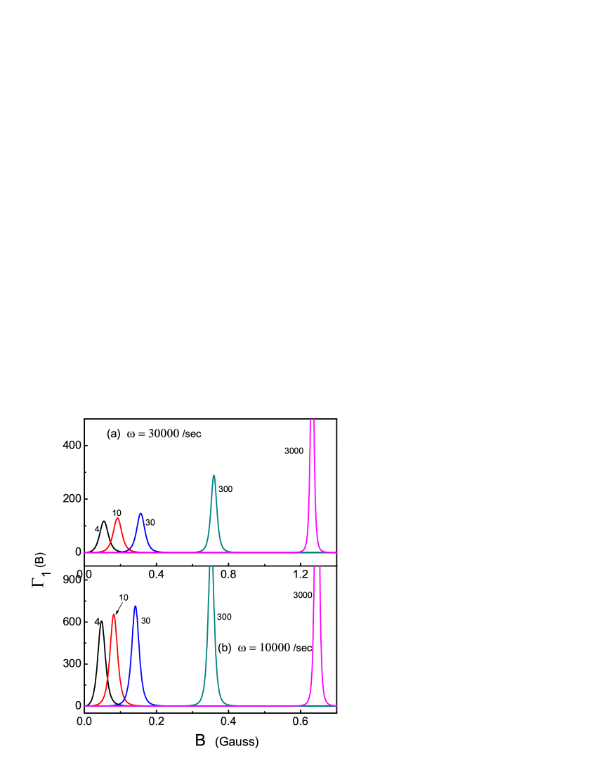
Figure 1: (color on line) The fidelity susceptibility
of the g.s. of the 2-level system of Na versus
. (a) and
(b), and is given at five values marked by
the curves. Note that the scales of are different in (a)
and (b).
We first study the susceptibility of the two eigenstates
against . The fidelity susceptibility is defined as
14quan06
(10)
For Na, of the g.s. distinct in are plotted
in Fig.1. Due to the fact that , and
, , i.e., both
states have exactly the same susceptibility. This is a spacial
feature dedicated only to 2-level systems. There are sharp
peaks in Fig.1 implying that the system is inert to in
general, but extremely sensitive when falls in the specific
narrow domains, namely, the domain of sensitivity (D-o-S). The
location of the peak is denoted as which varies with
and/or . The left and right borders of the D-o-S
are named and . They can be roughly
defined as
.
A larger will lead to a higher and narrower peak shifted to
the right, while a larger will lead to a lower and
broader peak also shifted to the right.
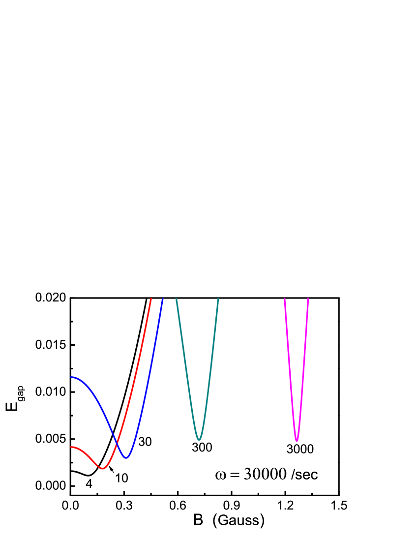
Figure 2: of the 2-level system versus .
is assumed. Refer to Fig.1a.
is plotted in Fig.2. For each , has a
minimum located at (). From ,
(11)
(for Na, and fulfill the relation
, where is in and is in
1sten98 ). By comparing Fig.2 and 1a, we found
that . They are closer to each other when
is larger (say, , 0.0003, and 0 when
, , and 3000, respectively). In fact, when we expand
via a perturbation series, we found
that , thus a smaller gap
will lead to a higher sensitivity. Eq. (11) explain why
a larger will lead to a larger . Furthermore, a
larger will lead to a more compact ,
and therefore a larger and a larger as well.
Eq.(11) provides a convenient way to evaluate the
location of the D-o-S. When is large, under the
Thomas-Fermi approximation, .
Accordingly, . Thus
increases with slowly but increases with rapidly
as shown in Fig.1.
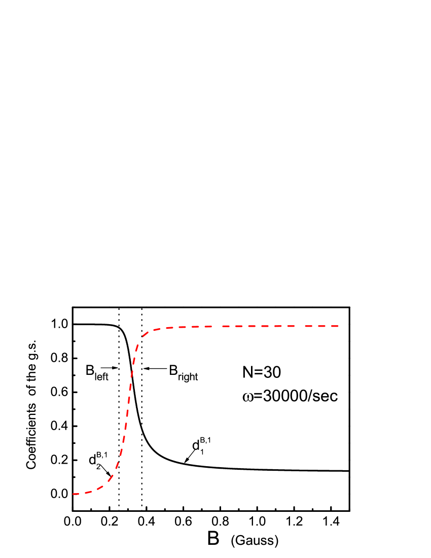
Figure 3: The coefficients (solid) and
(dash) of the g.s. versus . and
are assumed.
The variation of the g.s. versus is shown in Fig.3. The
D-o-S appearing in Fig.1a appears again in Fig.3, wherein the
coefficients and undergo a sharp
change. When , remains
implying that the effect of is effectively hindered by the
gap. When , we found that
.
Where is a Fock-state in the
spin-space having particles in . Note that, when
, in a g.s. should be maximized
(under the conservation of ) to reduce the quadratic Zeeman
energy. Therefore, should tend to the above limit.
Whereas the excited state . From Fig.3 we
know that, when increases, the spin-state of the g.s. is
changed from to and the
change happens essentially inside the D-o-S. Accordingly,
matching the change of the g.s., the excited state is changed
from to .
Figure 4: (solid), (dash), (dash-dot) and
(dash-dot-dot) versus . (a to
e) and (f), and is given at five values
marked in each panel. In the zone below the spatial
excitation can be neglected. In the zone below the system
remains in the g.s.. In the zone between and , the
thermo-fluctuation is saturated.
When the system has arrived at thermo-equilibrium under a given
temperature . If is very low, the spatial excitation is
negligible and the system would be essentially distributed
among the above two eigenstates. Since the energy for spatial
excitation (in ), the ratio is crucial, where . We define and at which and 100,
respectively. When , the effect of spatial excitation is
small, when , the effect of spatial excitation is
negligible. Thus, when the partition function of the
system is simply . The
probability that the system lies at the g.s. is . We
define further a turning temperature at which
. When , not only the spatial but also the
spin degrees of freedom are nearly frozen. Thus marks
the temperature of the secondary
condensation.15pasq12 ; 16li13 Let which is the probability lying at the excited
state. Note that when , an ideal 2-level
system would have . Thus we define the
second turning temperature at which . When , the thermo-fluctuation
is close to be saturated. The variations of ,
together with and versus are plotted in Fig.4.
From the definitions of and , one can prove
that they will also arrive at their minimum at as shown
in Fig.4. When is explicitly lower than , the 2-level
system can be safely considered as a pure spin-system.
The internal energy relative to the g.s. is
(12)
When is fixed, would be zero
if and if . For
the latter case, and arrives at a
maximum , where is a
characteristic constant dedicated to 2-level systems
disregarding , , and the parameters of interaction.
Note that is the energy assigned to
the spatial motion of only a single particle, while is the
total spin energy (relative to the g.s.). Thus the very small
upper limit manifests how weak the energy is
involved.
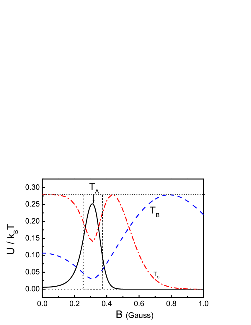
Figure 5: versus . and
are assumed. The solid, dash, and dash-dot lines are for
, , and (refer to the text), respectively.
The two vertical dotted lines mark the D-o-S, and the
horizontal dotted line marks the upper limit.
An example of versus (associated with Fig.4c) are
plotted in Fig.5. is given at three values,
,
, and . When
and increases from ,
it is clear from Fig.4c that appears as a small
peak. It implies that undergoes an increase and
afterward a decrease. Accordingly, is peaked in the D-o-S
as shown by the solid line in Fig.5. Whereas when and
from , the system will enter
to the zone where the thermo-fluctuation is saturated, and
therefore will remains unchanged. In this case the
variation of is largely contributed by . The dip
in (refer to Fig.2) leads to the dip in as shown
by the dash curve in Fig.5. When is larger, the increase of
remains, and thereby keeps increasing until it
arrives at its upper limit . When is larger
further, it is shown in Fig.4c that the system will tend to the
g.s. so that will tend to zero. It is notable that in all
cases holds as shown by the horizontal
dotted line.
The probability of a particle in in the state,
according to Eq.(9) of ref.13bao12 , is
(13)
Taking the thermo-fluctuation into account, we define the weighted
probability as
(14)
Figure 6: , the weighted
probability of a particle in , versus B for the case of
Fig.4c. Refer to Fig.5.
For the case of Fig.4c, is plotted in Fig.6,
where changes sharply inside the D-o-S when
. Furthermore, it was found that
when . It arises because
meanwhile the spin-state is equal to
, where
is for the g.s. (excited state). Therefore,
disregarding . Accordingly, the
three curves distinct in converge at . Once
has been measured at distinct , from the
point of convergency one can know and , the latter is
related to the dynamic parameters. When is sufficiently
large, from Fig.4, the system might fall into the g.s., and
accordingly as shown in Fig.6.
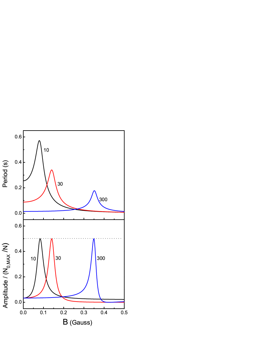
Figure 7: Period (a) and the amplitude (b) of population
oscillation of Na atoms versus . is assumed
and is given at three values marked by the curves. The unit
of the amplitude is , where is the
maximal number of particles.
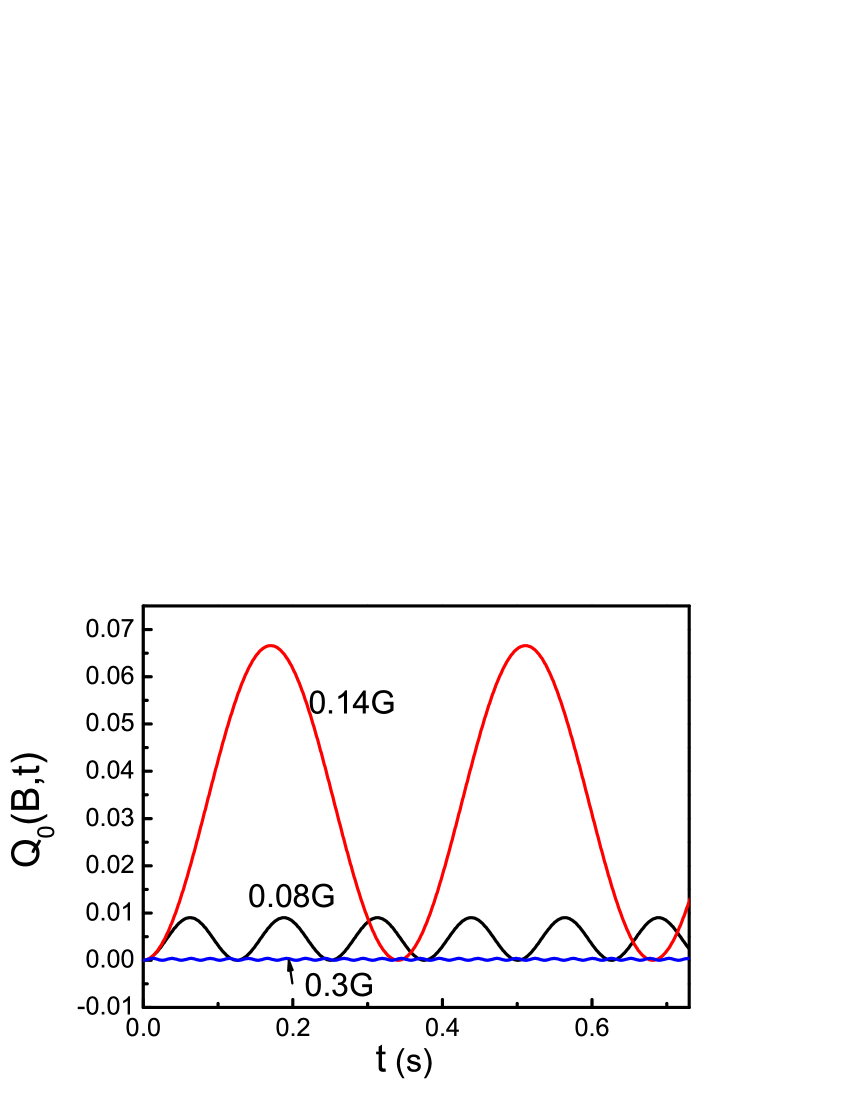
Figure 8: Population oscillation of Na atoms versus
(in ). and are given. is
given at three values marked by the curves (where, ,
refer to Fig.1b).
There are a number of experiments related to the early stage of
spin-evolution.2chan05 ; 3blac07 ; 4kron05 ; 5kron06 ; 6higb05 ; 7wide05 ; 8wide06 ; 9pech13
Starting from an initial state , the system
will evolve as , where
and denote the eigenenergy and eigenstate,
respectively.17chen09 In general there are infinite
eigenstates but only two for our two-level system. Thereby
has simple analytical form. Let the eigenstate be
re-expanded by the Fock-states as , . Obviously,
and , they depend
on . When the initial state is so prepared that
(Namely, particles are
prepared in spin up, then one down-particle is added), the
time-dependent probability of a particle in is
17chen09
(15)
where the amplitude .
Eq.(15) provides a clear picture of population
oscillation with the period .
Examples on and are given in Fig.7. There are peaks
in both 7a and 7b implying strong oscillation. They match
exactly with the peaks in Fig.1b. However, outside the D-o-S,
the amplitude is very small. When ,
, and therefore
. and the number of particles oscillates from 0 to its maximum
(refer to the horizontal dotted line in 7b). It is emphasized
that, for the given initial state, can arrives at its
maximum only when . When ,
while
and .
Therefore as shown in 7a, and as shown in 7b, and the oscillation damps. The oscillation
of versus is shown in Fig.8. The fact that a
slight change of around leads to a great change in
the population oscillation is notable.
In summary, a two-level system of cold sodium atoms has been
studied. The following features are found.
(i) The system is inert to in general, but very sensitive
in a specific domain (D-o-S), where appears as a
sharp peak, and appears as a dip. The locations of
the D-o-S can be predicted and can be tuned by changing
and/or .
(ii) When is sufficiently low, the system is free from the
interference of spatial excitation. There is a characteristic
constant dedicated to 2-level systems.
Accordingly, the upper limit of the internal energy
(relative to the g.s.) is . It implies that the
of the whole -body system is even ,
the energy assigned to a single spatial degrees of freedom.
(iii) When (where the dip of locates at),
distinct in converge at . Once
can be measured, the messages on , ,
and thereby the dynamic parameters can be obtained.
(iv) The spin-evolution depends strongly on . When
, the amplitude of oscillation is small (Fig.7).
When , the oscillation damps due to the sustained
increasing of the . When falls into the D-o-S, a
strong oscillation emerges. Thereby valuable message on the
dynamic parameters can be extracted.
(v) We have found a number of distinguished features for Na.
The crucial point is the existence of the minimum in .
Note that
while .
Therefore, when is small, the g.s. dominated by
contains more particles
than the excited state contains. Thus the increase of Zeeman
energy in the g.s. is faster than that in the excited state.
This leads to a decline of the gap. Such a decline will be
ended at at which of both states are the same.
Whereas, for Rb, the g.s. contains fewer particles.
Thus the decline of the gap in accord with the increase of
does not happen. Accordingly, the minimum of the gap is located
at . Hence, the 2-level systems of Rb would have
completely different features.
In this paper we have not considered the interference of
spatial excitation. In a recent paper it is reported that some
features of a gas of Na atoms with multi-spatial-mode can be
explained based on a theory independent of the spatial degrees
of freedom.9pech13 Similar features between Fig.2 of
that paper and Fig.7 of our paper are found. Nonetheless, when
, how serious the spatial-mode would affect the
spin-motion of our 2-level system deserves to be further
studied.
Acknowledgements.
The project is supported by the
National Basic Research Program of China (2008AA03A314,
2012CB821400, 2013CB933601), NSFC projects (11274393,
11074310, 11275279), RFDPHE of China (20110171110026) and
NCET-11-0547.
References
(1)
J. Stenger, et al., Nature 396, 345 (1998).
(2)
M. S. Chang, Q. Qin, W. X. Zhang, L. You, and M. S. Chapman,
Nature Physics 1, 111 (2005).
(3)
A. T. Black, E. Gomez, L. D. Turner, S. Jung, and P. D. Lett,
Phys. Rev. Lett. 99, 070403 (2007).
(4)
J. Kronjäer, C. Becker, M. Brinkmann, R. Walser, P. Navez, K. Bongs, and K. Sengstock,
Phys. Rev. A 72, 063619 (2005).
(5)
J. Kronjäer, C. Becker, P. Navez, K. Bongs, and K. Sengstock,
Phys. Rev. Lett. 97, 110404 (2006).
(6)
J. M. Higbie, L. E. Sadler, S. Inouye, A. P. Chikkatur, S.R. Leslie, K. L. Moore, V. Savalli, and D. M. Stamper-Kurn,
Phys. Rev. Lett. 95, 050401 (2005).
(7)
A. Widera, F. Gerbier, S. Föling, T. Gericke, O. Mandel,and I. Bloch,
Phys. Rev. Lett. 95, 190405 (2005).
(8)
A. Widera, F. Gerbier, S. Föling, T. Gericke, O. Mandel,and I. Bloch,
New J. Phys. 8, 152 (2006).
(9)
H. K. Pechkis, J. P. Wrubel, A. Schwettmann, P. F. Griffin, R. Barnett, E. Tiesinga, and P. D. Lett,
Phys. Rev. Lett. 111, 025301 (2013).
(10)
J. Katriel,
Mol. Struct.:THEOCHEM 547,1 (2001).
(11)
C. G.Bao and Z. B. Li,
Phys. Rev. A 70, 043620 (2004).
(12)
C. G. Bao and Z. B. Li,
Phys. Rev. A 72, 043614 (2005).
(13)
C. G. Bao,
J. Phys. A:Math. Theor. 45, 235002 (2012).
(14)
H. T. Quan, Z. Song, X. F. Liu, P, Zanardi, and C. P. Sun,
Phys. Rev. Lett. 96, 140604 (2006);
W.-L. You, Y.-W. Li, and S.-J. Gu,
Phys. Rev. E 76, 022101 (2007).
(15)
B. Pasquiou, E. Maréchal, L. Vernac, O. Gorceix, and B. Laburthe-Tolra,
Phys. Rev. Lett. 108, 045307 (2012).
(16)
Z. B. Li, D. X. Yao, C. G. Bao,
arXiv:1309.1933 [cond-mat,stat-mech], 2013.
(17)
Z. F. Chen, C. G. Bao, and Z. B. Li,
J. Phys. Soc. Japan, 78, 114002 (2009).