Recurrence Relations for Graph Polynomials on Bi-iterative Families of Graphs

Abstract.

We show that any graph polynomial from a wide class of graph polynomials yields a recurrence relation on an infinite class of families of graphs. The recurrence relations we obtain have coefficients which themselves satisfy linear recurrence relations. We give explicit applications to the Tutte polynomial and the independence polynomial. Furthermore, we get that for any sequence $a_{n}$ satisfying a linear recurrence with constant coefficients, the sub-sequence corresponding to square indices $a_{n^{2}}$ and related sub-sequences satisfy recurrences with recurrent coefficients.

1. Introduction

Recurrence relations are a major theme in the study of graph polynomials. As early as 1972, N. L. Biggs, R. M. Damerell and D. A. Sands [4] studied sequences of Tutte polynomials which are C-finite, i.e. satisfy a homogenous linear recurrence relation with constant coefficients (or equivalently, sequences of coefficients of rational power series). More recently, M. Noy and A. Ribó [23] proved that over an infinite class of recursively constructible families of graphs, which includes e.g. paths, cycles, ladders and wheels, the Tutte polynomial is C-finite (see also [5]). The Tutte polynomials of many recursively constructible families of graphs received special treatment in the literature. Moreover, the Tutte polynomial can be defined through its famous deletion-contraction recurrence relation.

Similar recurrence relations have been studied for other graph polynomials, e.g. for the independence polynomial see e.g. [19, 29]. E. Fischer and J. A. Makowsky [11] extended the result of Noy and Ribó to an infinite class of graph polynomials definable in Monadic Second Order Logic (MSOL), which includes the matching polynomial, the independence polynomial, the interlace polynomial, the domination polynomial and many of the graph polynomials which occur in the literature. [11] applies to the wider class of iteratively constructible graph families. The class of MSOL-polynomials and variations of it were studied with respect to their combinatorial and computational properties e.g. in [7, 16, 18, 22]. L. Lovász treats MSOL-definable graph invariants in [20].

In this paper we consider recurrence relations of graph polynomials which go beyond C-finiteness. A sequence is C${\,}^{2}$-finite if it satisfies a linear recurrence relation with C-finite coefficients. We start by investigating the set of C²-finite sequences. The tools we develop apply to sparse sub-sequences of C-finite sequences. While C-finite sequences have received considerable attention in the literature, cf. e.g. [26, Chapter 4], and it is well-known that taking a linear sub-sequence $a_{qn+r}$ of a C-finite sequence $a_{n}$ yields again a C-finite sequence, it seems other types of sub-sequences have not been systematically studied. We show the following:

Theorem 1.

Let $a_{n}$ be a C-finite over $\mathbb{C}$. Let $c\in\mathbb{N}^{+}$ and $d,e\in\mathbb{Z}$. Then the sequence

$$b_{n}=a_{c\binom{n}{2}+dn+e}$$

is C${\,}^{2}$-finite.

In particular, $a_{n^{2}}$ and $a_{\binom{n}{2}}$ are C²-finite. The proof of Theorem 1 is given in Section 3. As an explicit example, we consider the Fibonacci numbers in Section 4.

Next, we show MSOL-polynomials satisfy C²-recurrences on appropriate families of graphs. In Section 5 we introduce the notion of bi-iteratively constructible graph families, or bi-iterative families for short. In Section 6 we recall from the literature the definitions of two related classes of MSOL-polynomials and introduce a powerful theorem for them. The main theorem of the paper is:

Theorem 2 (Informal).

MSOL-polynomials satisfy C${\,}^{2}$-finite recurrences on bi-iterative families.

Theorem 2 shows the existence of the desired recurrence relations. The exact statement Theorem 2, namely Theorem 32, is given in Section 7 together with the proof. In Section 8 we compute explicit C²-recurrences for the Tutte polynomial and the independence polynomial. Finally, in Section 9 we conclude and discuss future research.

2. C²-finite sequences

In this section we define the recurrence relations we are interested in and give useful properties of sequences satisfying them.

Definition 3.

Let $\mathbb{F}$ be a field. Let $a_{n}:\,n\in\mathbb{N}$ be a sequence over $\mathbb{F}$.

1. $a_{n}$ is C-finite if there exist $s\in\mathbb{N}$ and $c^{(0)},\ldots,c^{(s)}\in\mathbb{F}$, $c^{(s)}\not=0$, such that for every $n\geq s$,

   $$c^{(s)}a_{n+s}=c^{(s-1)}a_{n+s-1}+\cdots+c^{(0)}a_{n}\,.$$

   We may assume w.l.o.g. that $c^{(s)}=1$.

2. $a_{n}$ is P-recursive if there exist $s\in\mathbb{N}$ and $c_{n}^{(0)},\ldots,c_{n}^{(s)}$ which are polynomials in $n$ over $\mathbb{F}$, such that for every $n$ we have $c_{n}^{(s)}\not=0$, and for every $n\geq s$,

   (2.1) $$c_{n}^{(s)}a_{n+s}=c_{n}^{(s-1)}a_{n+s-1}+\cdots+c_{n}^{(0)}a_{n}\,.$$

3. $a_{n}$ is C²-finite if there exist $s\in\mathbb{N}$ and C-finite sequences $c_{n}^{(0)},\ldots,c_{n}^{(s)}$, such that for every $n$ we have $c_{n}^{(s)}\not=0$, and for every $n\geq s$ , Eq. (2.1) holds.

P-recursive (holonomic) sequences have been studied in their own right, but also as the coefficients of Differentially finite generating functions [27], see also [24].

Example 4 (C²-finite sequences).

Sequences with C²-finite recurrences emerge in various areas of mathematics.

1. The $q$-derangement numbers $d_{n}(q)$ are polynomials in $q$ related to the set of derangements of size $n$. A formula for computing them in analogy to the standard derangement numbers was found by I. Gessel [15] and M. L. Wachs [28]. This formula implies that the following C²-recurrence holds:

   $$d_{n}(q)=(q^{n}+[n])d_{n-1}(q)-q^{n}[n]d_{n-2}(q)\,,$$

   see also [10]. We denote here $[n]=1+q+q^{2}+\cdots+q^{n-1}$.

2. In knot theory, the colored Jones polynomial of a framed knot $\mathcal{K}$ in $3$-space is a function from such knots to polynomials. The colored Jones function of the $0$-framed right-hand trefoil satisfies the following C²-recurrence [12]:

   $$J_{\mathcal{K}}(n) = \frac{x^{2n-2}+x^{8}y^{4n}-y^{n}-x^{2}y^{2n}}{x(x^{2n}y-x^{4}y^{n})}J_{\mathcal{K}}(n-1)$$

   $$+\frac{x^{8}y^{4n}-x^{6}y^{2n}}{x^{4}y^{n}-x^{2n}y}J_{\mathcal{K}}(n-2)$$

   with $x=q^{1/2}$ and $y=x^{-2}$. See [13] and [14] for more examples.

Lemma 5 (Properties).

1. Every C-finite sequence is P-recursive.

2. Every P-recursive sequence is C²-finite.

3. For every C-finite sequence $a_{n}$, there exists $\alpha\in\mathbb{N}$ such that $a_{n}\leq\alpha^{n}$ for every large enough $n$.

4. For every P-recursive sequence $a_{n}$, there exists $\alpha\in\mathbb{N}$ such that $a_{n}\leq n!^{\alpha}$ for every large enough $n$.

5. For every C${\,}^{2}$-finite sequence $a_{n}$, there exists $\alpha\in\mathbb{N}$ such that $a_{n}\leq\alpha^{n^{2}}$ for every large enough $n$.

Proof.

1 and 2 follow directly from Definition 3. 3, 4 and 5 can be proven easily by induction on $n$. ∎

The following will be useful, see e.g. [26]:

Lemma 6 (Closure properties).

The C-finite sequences are closed under:

1. Finite addition;

2. Finite multiplication;

3. Given a C-finite sequence $a_{n}$, taking sub-sequences $a_{tn+s}$, $t\in\mathbb{N}^{+}$ and $s\in\mathbb{Z}$.

The sets of C-finite sequences and P-recursive sequences form rings with respect to the usual addition and multiplication. However, they are not integral domains. For every $i\leq p$ and every $n$ let

$$\mathbb{I}_{n\equiv i\,(mod\,p)}=\begin{cases}1&n\equiv i\,(mod\,p)\\ 0&n\not\equiv i\,(mod\,p)\end{cases}$$

For every $i\leq p$, $\mathbb{I}_{n\equiv i\,(mod\,p)}$ is C-finite. While each of $\mathbb{I}_{n\equiv 0\,(mod\,2)}$ and $\mathbb{I}_{n\equiv 1\,(mod\,2)}$ is not identically zero, their product is. This obsticale complicates our proofs in the sequel, and is overcome using a classical theorem on the zeros of C-finite sequences:

Theorem 7 (Skolem-Mahler-Lech Theorem).

If $a_{n}$ is C-finite, then there exist a finite set $I\subseteq\mathbb{N}$, $n_{1},p\in\mathbb{N}$, and $P\subseteq\{0,\ldots,p-1\}$ such that

$$\{n\mid a_{n}=0\}=I\cup\bigcup_{i\in P}\{n\mid n>n_{1},\,n\equiv i\,(mod\,p)\}\,.$$

Remark 8.

Recently J. P. Bell, S. N. Burris and K. Yeats [2] extended the Skolem-Mahler-Lech theorem extends to a Simple P-recursive sequences, P-recursive sequences where the leading coefficient is a constant.

2.1. C-finite matrices

A notion of sequences of matrices whose entries are C-finite sequences will be useful. We define this exactly and prove some properties of these matrices sequences.

Definition 9.

Let $r\in\mathbb{N}$ and let $\left\{A_{n}\right\}_{n=1}^{\infty}$ be a sequence of $r\times r$ matrices over a field $\mathbb{F}$. We say $\left\{A_{n}\right\}_{n=1}^{\infty}$ a C-finite matrix sequence if for every $1\leq i,j\leq r$, the sequence $A_{n}[i,j]$ is C-finite.

Lemma 10.

Let $r,n_{0}\in\mathbb{N}$ and let $\left\{A_{n}\right\}_{n=n_{0}}^{\infty}$ be a C-finite matrix sequence of $r\times r$ matrices over $\mathbb{C}$. The following hold:

1. The sequence $\left\{A_{n}^{T}\right\}_{n=1}^{\infty}$ is an C-finite matrix sequence.

2. The sequence $\left\{\left|A_{n}\right|\right\}_{n=1}^{\infty}$ is in C-finite.

3. For any fixed $i,j$, the sequence of consisting of the $(i,j)$-th cofactor of $A_{n}$ is C-finite, and the sequence $\left\{C_{n}\right\}_{n=1}^{\infty}$ of matrices of cofactors of $A_{n}$ is an C-finite matrix sequence.

4. There exist $n_{1}$ and $p$ such that, for every $0\leq i\leq p-1$ and $n\in\mathbb{N}^{+}$, $\left|A_{i+n_{1}}\right|=0$ iff $\left|A_{pn+i+n_{1}}\right|=0$.

5. Let $n_{1},p\in\mathbb{N}$. If $\left|A_{pn+i+n_{1}}\right|\not=0$ for every $n\in\mathbb{N}^{+}$, then the sequence of matrices of the form $\left(A_{pn+i+n_{1}}\right)^{-1}$ is an C-finite matrix sequence.

Proof.

1. Immediate.

2. The determinant is a polynomial function of the entries of the matrix, so it is C-finite by the closure of the set of C-finite sequences to finite addition and multiplication.

3. The cofactor is a constant times a determinant, so again it is C-finite.

4. This follows from the Lech-Mahler-Skolem property of C-finite sequences and from the fact that the determinant is a C-finite sequence.

5. The transpose of the matrix of cofactors $C_{n}$ of $A_{n}$ is an C-finite matrix sequence by the above. Since $\left|A_{pn+i+n_{1}}\right|\not=0$ for every $n\in\mathbb{N}^{+}$, then the $\left(A_{pn+i+n_{1}}\right)^{-1}=\frac{1}{\left|A_{pn+i+n_{1}}\right|}C_{n}$ is well-defined and an C-finite matrix sequence.

∎

Lemma 11.

Let $M$ be an $r\times r$ matrix. Let $c,d\in\mathbb{Z}$ with $c>0$. Let

$$M_{n}=\begin{cases}M^{cn+d},&cn+d\geq 0\\ 0,&\mbox{otherwise}\end{cases}$$

The sequence $M_{n}$ is a C-finite matrix sequence.

Proof.

Let

$$\chi(\lambda)=\sum_{t=0}^{r}e_{t}\lambda^{t}$$

be the characteristic polynomial of $M^{c}$, with $e_{r}\not=0$. By the Cayley-Hamilton theorem, $\chi(M^{c})=0$, so

(2.2) $$0=\sum_{t=1}^{r}e_{t}M^{ct}$$

with $e_{r}\not=0$. If $d\geq 0$, then by multiplying Eq. (2.2) by $M^{d}$ and setting $t=n$, we get that for every $i,j$, the entry $(i,j)$ in the sequence of matrices $M_{n}:\,n\in\mathbb{N}$ satisfies the recurrence

$$M_{n}[i,j]=-\sum_{t=1}^{r-1}\frac{e_{t}}{e_{r}}M_{n-r+t}[i.j]\,.$$

If $d<0$, there exists $r>0$ such that $cr>|d|$. We have $M^{cn+d}=M^{c(n-r)+cr-|d|}$. The claim follows similarly to the case of $d\geq 0$ by multiplying Eq. (2.2) by $M^{cr-|d|}$ and setting $t=n-r$. ∎

Lemma 12.

Let $r,m,\ell\in\mathbb{N}$ and let $\left\{A_{n}\right\}_{n=n_{0}}^{\infty}$, $\left\{B_{n}\right\}_{n=n_{0}}^{\infty}$ be C-finite matrix sequences of consisting of matrices of size $r\times m$ respectively $m\times\ell$ over $\mathbb{C}$. Then $A_{n}B_{n}$ is an C-finite matrix sequence.

Proof.

Let $1\leq i\leq r$ and $1\leq j\leq\ell$. Then

$$\left(A_{n}B_{n}\right)_{ij}=\sum_{k=1}^{m}\left(A_{n}\right)_{ik}\left(B_{n}\right)_{kj}$$

is a polynomial in C-finite matrix sequences. Hence, by the closure of C-finite sequences to finite addition and multiplication, $A_{n}B_{n}$ is an C-finite matrix sequences. ∎

3. Proof of Theorem 1

The proof of Theorem 1 relies on the notion of a pseudo-inverse of a matrix. This notion is a generalization of the inverse of square matrices to non-square matrices. For an introduction, see [3]. We need only the following theorem:

Theorem 13 (Moore-Penrose pseudo-inverse).

Let $\mathbb{F}$ be a subfield of $\mathbb{C}$. Let $s,t\in\mathbb{N}^{+}$. Let $M$ be a matrix over $\mathbb{F}$ of size $s\times t$ with $s\geq t$ whose columns are independent. Then there exists a unique matrix $M^{+}$ over $\mathbb{F}$ of size $t\times s$ which satisfies the following conditions:

1. $M^{*}M$ is non-singular;

2. $M^{+}=\left(M^{*}M\right)^{-1}M^{*}$;

3. $M^{+}M=I$.

$M^{*}$ is the Hermitian transpose of $M$, i.e. $M^{*}$ is obtained by taking the transpose of $M$ and replacing each entry with its complex conjugate.

$M^{+}$ is called the Moore-Penrose pseudo-inverse of $M$.

The following is the main lemma necessary for the proof of Theorem 1. It allows to extract C²-recurrences for individual sequences of numbers from recursion schemes with C-finite coefficients for multiple sequences of numbers.

Lemma 14.

Let $\mathbb{F}$ be a subfield of $\mathbb{C}$ and let $r\in\mathbb{N}^{+}$. For every $n\in\mathbb{N}^{+}$, let $\overline{v_{n}}$ be a column vector of size $r\times 1$ over $\mathbb{F}$. Let $w_{n}$ be a C-finite sequence which is always positive. Let $M_{n}$ be an C-finite matrix sequence consisting of matrices of size $r\times r$ over $\mathbb{F}$ such that, for every $n$,

(3.1) $$\overline{v_{n+1}}=\frac{1}{w_{n}}M_{n}\overline{v_{n}}\,.$$

For each $j=1,\dots,r$, $\overline{v_{n}}[j]$ is C${\,}^{2}$-finite. Moreover, all of the $\overline{v_{n}}[j]$ satisfy the same recurrence relation (possibly with different initial conditions).

Proof.

For every $i=0,\ldots,r^{2}$, let $M_{n}^{\{i\}}=\frac{1}{w_{n+i-1}\cdots w_{n-1}}M_{n+i-1}\cdots M_{n-1}$. By Eq. (3.1), for every $n$,

(3.2) $$\overline{v_{n+i}}=M_{n}^{\{i\}}\overline{v_{n-1}}\,.$$

Let $N_{n}^{\{0\}},\ldots,N_{n}^{\{r^{2}\}}$ be the column vectors of size $r^{2}\times 1$ corresponding to $M_{n}^{\{0\}},$$\ldots,M_{n}^{\{r^{2}\}}$ with $N_{n}^{\{i\}}[r(k-1)+\ell]=M^{\{i\}}[k,\ell]$. For every fixed $n$, $N_{n}^{\{0\}},\ldots,N_{n}^{\{r^{2}\}}$ are members of the vector space of column vectors over $\mathbb{F}$ of size $r^{2}\times 1$. Since this vector space is of dimension $r^{2}$, $N_{n}^{\{0\}},\ldots,N_{n}^{\{r^{2}\}}$ are linearly dependent. Let $s_{n}\in\{1,\ldots,r^{2}\}$ be such that $N_{n}^{\{s_{n}\}},\ldots,N_{n}^{\{r^{2}\}}$ are linearly independent, but $N_{n}^{\{s_{n}-1\}},$$\ldots,N_{n}^{\{r^{2}\}}$ are linearly dependent. We have that $N_{n,s_{n}}^{*}N_{n,s_{n}}$ is non-singular.

For every $t=0,\ldots,r^{2}-1$ let $N_{n,t}$ be the $r^{2}\times(r^{2}-t)$ matrix whose columns are $N_{n}^{\{t\}},\ldots,N_{n}^{\{r^{2}-1\}}$. Let

$$\widetilde{N_{n,t}}=C\left(N_{n,t}^{*}N_{n,t}\right)^{T}N_{n,t}^{*}$$

where $C\left(N_{n,t}^{*}N_{n,t}\right)^{T}$ is the transpose of the cofactor matrix of $N_{n,t}^{*}N_{n,t}$. Then

$$N_{n,s_{n}}^{+}=\frac{1}{|N_{n,s_{n}}^{*}N_{n,s_{n}}|}\widetilde{N_{n,s_{n}}}=\left(N_{n,s_{n}}^{*}N_{n,s_{n}}\right)^{-1}N_{n,s_{n}}^{*}$$

is the Moore-Penrose pseudo-inverse of $N_{n,s_{n}}$, where $|N_{n,t}^{*}N_{n,t}|$ denotes the determinant of the matrix. In particular,

(3.3) $$N_{n,s_{n}}^{+}N_{n,s_{n}}=I\,.$$

Consider the system of linear equations

(3.4) $$N_{n,s_{n}}y_{n,s_{n}}=N_{n}^{\{r^{2}\}}\,.$$

with $y_{n,s_{n}}$ a column vector of size $\left(r^{2}-s_{n}\right)\times 1$ of indeterminates $y_{n,s_{n}}[k]$. Let

$$y_{n,s_{n}}^{\prime} = \widetilde{N_{n,s_{n}}}N_{n}^{\{r^{2}\}}$$

$$y_{n,s_{n}} = \frac{1}{\left|N_{n,s_{n}}^{*}N_{n,s_{n}}\right|}y_{n,s_{n}}^{\prime}\,.$$

Using Eq. (3.3) we have that $y_{n,s_{n}}$ is a solution of Eq. (3.4). This solution which can be rephrased as the matrix equation:

(3.5) $$y_{n,s_{n}}^{\prime}[1]M_{n}^{\{s_{n}\}}+\cdots y_{n,s_{n}}^{\prime}[r^{2}-s_{n}]M_{n}^{\{r^{2}-1\}}=\left|N_{n,s_{n}}^{*}N_{n,s_{n}}\right|M_{n}^{\{r^{2}\}}\,.$$

Moreover, by Lemmas 12 and 10, $y_{n}^{\prime}$ is an C-finite vector sequence. Multiplying Eq. (3.5) from the right by $\overline{v_{n-1}}$ and rearranging, we get

(3.6) $$y_{n,s_{n}}^{\prime}[1]\overline{v_{n+s_{n}}}+\cdots y_{n,s_{n}}^{\prime}[r^{2}-s_{n}]\overline{v_{n+r^{2}-1}}-\left|N_{n,s_{n}}^{*}N_{n,s_{n}}\right|\overline{v_{n+r^{2}}}=0\,,$$

For every $n$ and every $s\geq s_{n}$, $\left|N_{n,s}^{*}N_{n,s}\right|\not=0$, and for every $s<s_{n}$, $\left|N_{n,s}^{*}N_{n,s}\right|=0$ are linearly dependent. By Claim 10, there exists $n_{1}$ such that for $n\geq n_{1}$, $s_{n}$ is periodic and let $p$ be the period. Using this periodicity we can remove the dependence of Eq. (3.6) on the infinite sequence $s_{n}$, and instead use for all $n\geq n_{1}$ a finite number of values, $s_{n_{1}+1},\ldots,s_{n_{1}+p}$:

$$\sum_{i=1}^{p}\mathbb{I}_{n\equiv i\,(mod\,p)}\Bigg{(}\Bigg{(}\sum_{j=1}^{r^{2}-s_{n_{1}+i}}y_{n,s_{n_{1}+i}}^{\prime}[j]\overline{v_{n+s_{n_{1}+i+j-1}}}\Bigg{)}$$

$$-\left|N_{n,s_{n_{1}+i}}^{*}N_{n,s_{n_{1}+i}}\right|\overline{v_{n+r^{2}}}\Bigg{)} = 0$$

which can be rewritten as

$$q_{n}^{\{0\}}\overline{v_{n}}+\cdots+q_{n}^{\{r^{2}-1\}}\overline{v_{n+r^{2}-1}}=q_{n}^{\{r^{2}\}}\overline{v_{n+r^{2}}}$$

with

$$q_{n}^{\{t\}}=\begin{cases}\sum_{i=1}^{p}\mathbb{I}_{n\equiv i\,(mod\,p)}y_{n,s_{n_{1}+i}}^{\prime}[t+1-s_{n_{1}+i}],\,\,\,&0\leq t\leq r^{2}-1\\ \sum_{i=1}^{p}\mathbb{I}_{n\equiv i\,(mod\,p)}\left|N_{n,s_{n_{1}+i}}^{*}N_{n,s_{n_{1}+i}}\right|,\,\,\,&t=r^{2}\,.\end{cases}$$

Note that, as the result of the closure of the C-finite sequences to finite addition and multiplication, $q_{n}^{\{t\}}$ is C-finite. Moreover, note $q_{n}^{\{r^{2}\}}$ is non-zero. ∎

We can now turn the main proof of this section.

Proof of Theorem 1.

Let $\zeta(n)=c\binom{n}{2}+dn+e$. Let $b_{n}^{\prime}=a_{\zeta(n)}$. We have

$$\zeta(n)-\zeta(n-1)=cn+d\,.$$

Let $a_{n}$ satisfy the C-recurrence

(3.7) $$a_{n+s}=c^{(s-1)}a_{n+s-1}+\cdots+c^{(0)}a_{n}\,.$$

In order to write the latter equation in matrix form, let

$$M=\left(\begin{array}[]{ccc}c^{(s-1)}&\cdots&c^{(0)}\\ 1\\ &\ddots\\ &&1\end{array}\right)$$

where the empty entries are taken to be $0$. Let $\overline{u_{n}}=\left(a_{n},\ldots,a_{n-s+1}\right)^{tr}$. We have

$$\overline{u_{n}}=M\overline{u_{n-1}}\,,$$

and consequently,

$$\overline{u_{\zeta(n)}}=M^{cn+d}\overline{u_{\zeta(n-1)}}\,.$$

For large enough values of $n$ such that $cn+d\geq 0$, $M^{cn+d}$ is C-finite by Lemma 11. Hence, the desired result follows from Lemma 14. ∎

As immediate consequences, we get closure properties for C²-finite sequences over $\mathbb{C}$.

Corollary 15.

Let $a_{n}$ and $b_{n}$ be C${\,}^{2}$-finite sequences. The following hold:

1. $a_{n}+b_{n}$ is C${\,}^{2}$-finite

2. $a_{n}b_{n}$ is C${\,}^{2}$-finite

Proof.

Let $a_{n}$ and $b_{n}$ satisfy the following recurrences

$$c_{n}^{(s)}a_{n+s} = c_{n}^{(s-1)}a_{n+s-1}+\cdots+c_{n}^{(0)}a_{n}$$

$$d_{n}^{(s)}b_{n+s^{\prime}} = d_{n}^{(s^{\prime}-1)}b_{n+s^{\prime}-1}+\cdots+d_{n}^{(0)}b_{n}$$

where the sequences $c_{n}^{(i)}$ and $d_{n}^{(i)}$ are C-finite and $c_{n}^{(s)}$ and $d_{n}^{(s)}$ are non-zero. It is convenient to assume without loss of generality that $s=s^{\prime}$. We apply Lemma 14 for both cases:

1. For $a_{n}+b_{n}$, let $\overline{v_{n+1}}=\left(a_{n+1},\ldots,a_{n+2-s},b_{n+1},\ldots,b_{n+2-s}\right)^{tr}$ and

   $$M=\frac{1}{c_{n}^{(s)}d_{n}^{(s)}}\left(\begin{array}[]{cccccc}c_{n+1}^{(s-1)}d_{n}^{(s)}&\cdots&c_{n+2-s}^{(0)}d_{n}^{(s)}&d_{n+1}^{(s-1)}c_{n}^{(s)}&\cdots&d_{n+2-s}^{(0)}c_{n}^{(s)}\\ d_{n}^{(s)}\\ &\ddots\\ &&d_{n}^{(s)}\\ &&&c_{n}^{(s)}\\ &&&&\ddots\\ &&&&&c_{n}^{(s)}\end{array}\right)$$

   where the empty entries are taken to be $0$. We have $\overline{v_{n+1}}=M\overline{v_{n}}$ and the claim follows from Theorem 14.

   1. For $a_{n}b_{n}$, we have

      (3.8) $$c_{n}^{(s)}d_{n}^{(s)}a_{n+s}b_{n+s} = \sum_{t_{1},t_{2}=0}^{s-1}c_{n}^{(t_{1})}d_{n}^{(t_{2})}a_{n+t_{1}}b_{n+t_{2}}\,.$$

      Let $\overline{v_{n+1}}=\left(a_{n+1-t_{1}}b_{n+1-t_{2}}:\,0\leq t_{1},t_{2}\leq s-1\right)^{tr}$. Similarly to the case of $a_{n}+b_{n}$, we can define $M$ such that $\overline{v_{n+1}}=\frac{1}{c_{n}^{(s)}d_{n}^{(s)}}M\overline{v_{n}}$, where the first row of $M$ corresponds to Eq. (3.8), and the subsequent rows consist of non-zero value and otherwise $0$s.

4. Fibonacci numbers

The Fibonacci number $F_{n}$, given by the famous recurrence

$$F_{n+2}=F_{n+1}+F_{n}$$

with $F_{1}=1,\,F_{2}=1$, can also be described in terms of counting binary words. $F_{n}$ counts the binary words of length $n-2$ which do not contain consecutive $1$s. Similarly, $F_{n-1}$ counts the binary words of length $n-2$ which begin with $0$ (or, equivalently, end with $0$), and $F_{n-2}$ counts the binary words which begin (end) with $1$. Let $W_{n}=F_{n+2}$.

Let $0<k<m$, then

$$W_{m+k}=W_{k-1}W_{m}+W_{k-2}W_{m-1}$$

since $W_{k-1}W_{m}$ counts the binary words of length $m+k$ with no consecutive $1$s which have $0$ at index $k$, and $W_{k-2}W_{m-1}$ counts the binary words with no consecutive $1$s which have $1$ at index $k$(and therefore $0$at index$k-1$. This translates back to the Fibonacci numbers as:

$$F_{m+k+2}=F_{k+1}F_{m+2}+F_{k}F_{m+1}$$

So we have for the appropriate choices of $m$ and $k$:

(4.1) $$F_{(n+1)^{2}} = F_{2n+1}F_{n^{2}+1}+F_{2n}F_{n^{2}}$$

$$F_{n^{2}} = F_{2n}F_{(n-1)^{2}}+F_{2n-1}F_{(n-1)^{2}-1}$$

$$F_{n^{2}+1} = F_{2n+1}F_{(n-1)^{2}}+F_{2n}F_{(n-1)^{2}-1}$$

Extracting $F_{(n-1)^{2}-1}$ from the second equation, we get:

$$F_{(n-1)^{2}-1} = \frac{F_{n^{2}}-F_{2n}F_{(n-1)^{2}}}{F_{2n-1}}$$

and substituting $F_{(n-1)^{2}-1}$ in the third equation, we have:

$$F_{n^{2}+1} = \frac{F_{2n}F_{n^{2}}+(F_{2n-1}F_{2n+1}-F_{2n}^{2})F_{(n-1)^{2}}}{F_{2n-1}}$$

and substituting into Eq. (4.1), we have

$$F_{2n-1}F_{(n+1)^{2}} = F_{2n}\left(F_{2n+1}+F_{2n-1}\right)F_{n^{2}}+F_{2n+1}\left(F_{2n-1}F_{2n+1}-F_{2n}^{2}\right)F_{(n-1)^{2}}$$

where $F_{2n-1}$, $F_{2n}\left(F_{2n+1}+F_{2n-1}\right)$ and $F_{2n+1}\left(F_{2n-1}F_{2n+1}-F_{2n}^{2}\right)$ are C-finite by the closure properties of C-finite sequences in Lemma 6. Similarly, we can derive the following C²-recurrence for $F_{\binom{n+1}{2}}$:

$$F_{n-1}F_{\binom{n+1}{2}} = \left(F_{n-1}F_{n+1}+F_{n}F_{n-2}\right)F_{\binom{n}{2}}+\left(F_{n}F_{n-1}^{2}-F_{n-2}F_{n}^{2}\right)F_{\binom{n-1}{2}}$$

The sequences $F_{n^{2}}$ and $F_{\binom{n}{2}}$ are catalogued in the On-Line Encyclopedia of Integer Sequences [1] as (A054783) and (A081667).

∎

5. Bi-iterative graph families

In this section we define the notion of a bi-iterative graph family, give examples for some simple families which are bi-iterative and provide some simple lemmas for them. The graph families we are interested in are built recursively by applying basic operations on $k$-graphs. A $k$-graph is of the form

$$G=\left(V,E;R_{1},\ldots,R_{k}\right)$$

where $\left(V,E\right)$ is a simple graph and $R_{1},\ldots,R_{k}\subseteq V$ partition $V$. The sets $R_{1},\ldots,R_{k}$ are called labels. The labels are used technically to aid in the description of the graph families, but we are really only interested in the underlying graphs. Before we give precise definitions and auxiliary lemmas for constructing bi-iterative graph families, we give some examples of bi-iterative graph families.

Figure 5.1. Examples of graphs belonging to the iterative families: paths, cycles, cliques, wheels, complete bipartite graphs and prisms. They are also bi-iterative families.

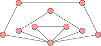
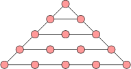
$G_{3}^{1}$	$G_{3}^{4}$
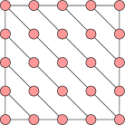
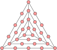
$G_{3}^{5}$	$G_{3}^{6}$

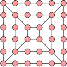
$G_{2}^{7}$

Figure 5.2. Examples of graphs belonging to some of the bi-iterative families of Example 16. The bi-iterative families $G_{n}^{1}$, $G_{n}^{4}$, $G_{n}^{5}$ and $G_{n}^{6}$ are bounded.

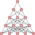
$G_{4}^{2}$	$G_{4}^{3}$

Figure 5.3. Examples of graphs belonging to the bi-iterative families of Example 16 not depicted in Figure 5.2. The bi-iterative families $G_{n}^{2}$ and $G_{n}^{3}$ are not bounded.

Example 16 (Bi-iterative graph families).

See Figures 5.1, 5.2 and 5.3 for illustrations of the following graph families.

1. Iteratively families, such as paths, cycles, and cliques, serve as simple examples of bi-iteratively constructible families.

2. $G_{0}^{1}$ is a single vertex labeled $2$. For each $n$, $G_{n}^{1}$ has one vertex labeled $2$ and all others are labeled $1$. $G_{n}^{1}$ is obtained from $G_{n-1}^{1}$ by adding a cycle of size $n+2$ and identifying one vertex of the cycle with the vertex labeled $2$ is in $G_{n-1}^{1}$. All other vertices in the cycle are labeled $1$.

3. $G_{n}^{2}$ is obtained from a path of length $n+1$ by adding, for each vertex $1\leq i\leq n+1$, a new clique of size $i$, and identifying one vertex of the clique with $i$.

4. $G_{0}^{3}$ is a single vertex labeled $2$. $G_{n}^{3}$ is obtained from $G_{n-1}^{3}$ by adding $n+1$ isolated vertices labeled $3$, adding all possible edges between vertices labeled $2$ and vertices labeled $3$, relabel all from $2$ to $1$, and then from $3$ to $2$.

5. $G_{0}^{4}$ consists of a triangle in which the vertices are labeled $1$,$2$,$3$. $G_{n}^{4}$ is obtained from $G_{n-1}^{4}$ by adding a path $P_{n+2}$ whose end-points are labeled $4$ and $5$. Then, the edges $\{2,4\}$ and $\{3,5\}$ are added, and the labels are changed so that the endpoints of the $P_{n+2}$ path are now labeled $2$ and $3$, and all other vertices in $G_{n}^{4}$ are labeled $1$.

6. $G_{0}^{5}$ is obtained by taking two disjoint copies of $G_{0}^{4}$ and respectively identifying the vertices labeled $2$ and $3$. $G_{n}^{5}$ is obtained from two disjoint copies of $G_{n-1}^{4}$ by adding a path $P_{n+2}$ and connecting each of its endpoints to the corresponding end-points labeled $2$ and $3$ of the two copies of $G_{n}^{5}$.

7. $G_{0}^{6}$ consists of a triangle in which the vertices are labeled $2$,$3$,$4$. $G_{n}^{6}$ is obtained by adding to $G_{n-1}^{6}$ a cycle of size $3n+3$ in which three vertices are labeled $5$,$6$,$7$. Between each of the pairs $(5,6)$, $(6,7)$ and $(5,7)$ there are $n$ vertices labeled $1$. Then, $2,3,4$ are connected to $5,6,7$ respectively, and the labels are changed so that only the vertices labeled $5,6,7$ remain labeled, and their new labels are $2,3,4$.

8. The family $G_{n}^{7}$ is similar to $G_{n}^{6}$, except we add a cycle of size $8n+4$, we have four distinguished vertices separated by $n$ vertices labeled $1$, etc.

Now we proceed to define the precise definitions which allow us to build such families.

Definition 17 (Basic and elementary operations).

The following are the basic operations on $k$-graphs:

1. $Add_{i}(G)$: A new vertex is added to $G$, where the new vertex belongs to $R_{i}$;

2. $\rho_{i\to j}(G)$: All the vertices in $R_{i}$ are moved to $R_{j}$, leaving $R_{j}$ empty;

3. $\eta_{i,j}(G)$: All possible edges between vertices labeled $i$ and vertices labeled $j$ are added;

4. $\eta_{i,j}^{b}(G)$: If $R_{i}\cup R_{j}\leq b$, then $\eta_{i,j}^{b}(G)=\eta_{i,j}(G)$; otherwise $\eta_{i,j}^{b}(G)=G$;

5. $\delta_{i,j}(G)$: All edges between vertices labeled $i$ and vertices labeled $j$ are removed.

An operation $F$ on $k$-graphs is elementary if $F$ is a finite composition of any of the basic operations on $k$-graphs. We denote by $id$ the elementary operation which leaves the $k$-graph unchanged.

Definition 18 (Bi-iterative graph families).

Let $k\in\mathbb{N}$, $G_{0}$ be a $k$-graph and $F,H,L$ be elementary operations on $k$-graphs,

1. The sequence $F(G_{n}):\,n\in\mathbb{N}$ is called an $F$-iteration family and is said to be an iteratively constructible family.

2. The sequence $G_{n+1}=H\left(F^{n}(L(G_{n}))\right):\,n\in\mathbb{N}$ is called an $(H,F,L)$-bi-iteration family and is said to be a bi-iteratively constructible family. By $F^{n}(G)$ we mean the result of performing $n$ consecutive applications of $F$ on $G$.

Let $G_{n}:\,n\in\mathbb{N}$ be a family of graphs. This family is (bi-)iteratively constructible if there exists $k\in\mathbb{N}$ and a family $G_{n}^{\prime}:\,n\in\mathbb{N}$ of $k$-graphs which is (bi-)iteratively constructible, such that $G_{n}$ is obtained from $G_{n}^{\prime}$ by ignoring the labels.

It is sometimes convenient to describe $G_{0}$ using basic operations on the empty graph $\emptyset$.

We can now prove the observation from Example 16(1):

Lemma 19.

Every iteratively constructible family is bi-iteratively constructible.

Proof.

If $F$ is an elementary operation such that $G_{n}:\,n\in\mathbb{N}$ is an $F$-iteration family, then $G_{n}:\>n\in\mathbb{N}$ is also an $(F,id,id)$-bi-iteration family. ∎

All of the families in Example 16 are bi-iteratively constructible families which are not iteratively constructible. The all grow too quickly to be iteratively constructible. Now consider for instance $G_{n}^{3}$. Let $F=Add_{3}$, $H=Add_{3}\circ\eta_{2,3}\circ\rho_{2\to 1}\circ\rho_{3\to 2}$ and $L=\emptyset$. We have $G_{n+1}^{3}=H(F^{n}(L(G_{n})))$.

In the sequel we will want to distinguish a particular type of bi-iterative families, in which every application of $\eta_{i,j}$ only adds at most a fixed amount of edges.

Definition 20 (Bounded bi-iterative families).

A basic operation is bounded if it not of the type $\eta_{i,j}$. A bi-iteratively constructible graph family $G_{n}:\,n\in\mathbb{N}$ is bounded if its construction uses only bounded basic operations.

Example 21.

Considering the families of Example 16, it is not hard to see that $G_{n}^{1}$, $G_{n}^{4}$, $G_{n}^{5}$,$G_{n}^{6}$,$G_{n}^{7}$ are bounded bi-iterative families, while $G_{n}^{2}$,$G_{n}^{3}$ are bi-iterative families which are not bounded.

5.1. Lemmas for building bi-iterative graph families

Here we give some lemmas which are useful to make the construction of bi-iterative families easier. Their aim is to help the reader understand which families of graph are bi-iterative.

Lemma 22.

Let $G_{n}^{A},G_{n}^{B}:\,n\in\mathbb{N}$ be two bi-iteratively constructible families. The family $G_{n}^{A}\sqcup G_{n}^{B}:\,n\in\mathbb{N}$ obtained by taking the disjoint union of the two families is bi-iteratively constructible. In particular, if both families $G_{n}^{A},G_{n}^{B}:\,n\in\mathbb{N}$ are iteratively constructible, then so is $G_{n}^{A}\sqcup G_{n}^{B}:\,n\in\mathbb{N}$.

Proof.

Let $H_{O},F_{O},L_{O}$ be elementary operations such that $G_{n}^{O}:\,n\in\mathbb{N}$ is an $(H_{O},F_{O},L_{O})$-bi-iteration family for $i=A,B$. We can assume w.l.o.g. that the labels of the two families are disjoint; if they are not, we can simply rename the labels used by one of the families. The family $G_{n}^{A}\sqcup G_{n}^{B}:\,n\in\mathbb{N}$ is an $(H_{A}\circ H_{B},F_{A}\circ F_{B},L_{A}\circ L_{B})$-bi-iteration family, where $\circ$ denotes the composition of operations. The case in which $G_{n}^{A},G_{n}^{B}:\,n\in\mathbb{N}$ are iteratively constructible is similar. ∎

Lemma 23.

Let $G_{n}:\,n\in\mathbb{N}$ and $J_{n}:\,n\in\mathbb{N}$ be iteratively constructible families of $k$-graphs whose basic operations use distinct labels. The family $G_{n}\sqcup J_{n}$ is an iteratively constructible family.

Proof.

Let $F_{G}$ and $F_{J}$ be the elementary operations associated with the two families. Let $F$ be the composition $F_{G}\circ F_{J}$. The iteratively constructible family whose underlying elementary operation is $F$ is $G_{n}\sqcup J_{n}$. ∎

Lemma 24.

Let $G_{n}:\,n\in\mathbb{N}$ be an iteratively constructible family of $k$-graphs and let $H$ and $L$ be two elementary operations over $k$-graphs. Let $D_{0}$ be a $k$-graph, and $D_{n+1}=H(L(D_{n})\sqcup G_{n})$. The family $D_{n}:\,n\in\mathbb{N}$ is bi-iteratively constructible.

Proof.

Let $F$ be an elementary operation such that $G_{n}:\,n\in\mathbb{N}$ is an $F$-iteration family. Let $F^{\prime}$ and $G_{0}^{\prime}$ be the same as $F$ and $G_{0}$, except that the labels they use are changed as follows. If a basic operation in $F$ uses label $i$, then the corresponding operation in $F^{\prime}$ uses label $i+k$. For every $i=1,\ldots,k$, let $\rho_{i}=\rho_{i\to i+k}$. Let $\rho$ be the composition $\rho_{1}\circ\cdots\circ\rho_{k}$. If a vertex in $G_{0}$ has label $i$, then the corresponding vertex in $G_{0}^{\prime}$ has label $i+k$. For every vertex $v$ of $G_{0}$ with label $i$, let $a_{v}=Add_{i+k}$. Let $a$ be the composition of $a_{v}$, $v\in V(G)$. We have $D_{n+1}=H(\rho(F^{\prime n}(a(L(D_{n})))))$, and therefore $D_{n}:\,n\in\mathbb{N}$ is a bi-iteratively constructible family of $2k$-graphs. ∎

Using Lemma 24, it is easy to show that some families from Example 16 are indeed bi-iterative.

Example 25.

Consider $G_{n}^{4}$ from Example 16. From Lemma 19 we get that $\tilde{P}_{n}=P_{n+3}^{4,5}$ is an iterative family. We define $E_{n+1}=H(L(E_{n})\sqcup\tilde{P}_{n})$ with $L=\rho_{1\to 5}\circ\rho_{2\to 6}$ and $H=\eta_{2,4}\circ\eta_{3,5}\circ\rho_{2\to 1}\circ\rho_{3\to 1}\circ\rho_{4\to 2}\circ\rho_{3\to 5}$. We get $G_{n}^{4}=E_{n}$.

Subfamilies of iteratively constructible families give rise to many other related bi-iteratively constructible families:

Lemma 26.

Let $G_{n}:\>n\in\mathbb{N}$ be iteratively constructible.

1. $G_{\binom{n}{2}}:\,n\in\mathbb{N}$ and $G_{n^{2}}:\,n\in\mathbb{N}$ are bi-iteratively constructible.

2. Let $c\in\mathbb{N}^{+}$ and $d,e\in\mathbb{Z}$. There exists $r\in\mathbb{N}$ such that $H_{n}=G_{cm^{2}+dm+e}:\,m\in\mathbb{N},\,m=n+r$ is bi-iteratively constructible.

Proof.

Let $F$ be an elementary operation such that $G_{n}:\,n\in\mathbb{N}$ is an $F$-iteration family.

1. $G_{\binom{n}{2}}:\,n\in\mathbb{N}$ is an $(id,F,id)$-bi-iteration family. The proof is by induction on $n$ with $G_{\binom{0}{2}}=G_{0}$ and

   $$id\left(F^{n}\left(id\left(G_{\binom{n}{2}}\right)\right)\right)=F^{n+\binom{n}{2}}\left(G_{0}\right)=F^{\binom{n+1}{2}}\left(G_{0}\right)=G_{\binom{n+1}{2}}\,.$$

   $G_{n^{2}}:\,n\in\mathbb{N}$ is an $(id,F^{2},F)$-bi-iteration family. Again by induction with $G_{0^{2}}=G_{0}$ and

   $$id\left(F^{2n}\left(F(G_{n^{2}})\right)\right)=F^{2n+1+n^{2}}\left(G_{0}\right)=F^{(n+1)^{2}}\left(G_{0}\right)=G_{(n+1)^{2}}\,.$$

2. Since $c>0$, there exists $r\in\mathbb{N}$ such that $c(n+r)^{2}+d(n+r)+e=cn^{2}+d^{\prime}n+e^{\prime}$ and $d^{\prime},e^{\prime}\geq 0$. Let $H_{0}=G_{e^{\prime}}$ , then $H_{n}:\,n\in\mathbb{N}$ is an $(id,F^{2c^{\prime}},F^{d^{\prime}+1})$-bi-iteration family. Here again the proof is by induction on $n$.

∎

5.2. Families which are not bi-iterative

Clique-width is a graph parameter which generalizes tree-width, and is very useful for designing efficient algorithms for NP-hard problems, see e.g. [9, 17].

Definition 27.

The clique-width $cwd(G)$ of a graph $G$ is the minimal $k\in\mathbb{N}$ such that there exists a $k$-graph $H$ whose underlying graph is isomorphic to $G$ and which can be obtained from $\emptyset$ by applying the basic operations $Add_{i}$, $\rho_{i\to j}$, $\eta_{i,j}$ and $\delta_{i,j}$ from Definition 17.

Bi-iterative families have bounded clique-width. Using this fact we easily get examples of families which are not bi-iterative.

Lemma 28.

If $G_{n}:\>n\in\mathbb{N}$ is a bi-iterative family of $k$-graphs, then for every $n$, $G_{n}$ has clique-width at most $k$.

Proof.

Let $G_{n}$ be a $(H,F,L)$-bi-iteration family of $k$-graphs. Since $G_{0}$ is a $k$-graph, it can be expressed by the basic operations $Add_{i}$, $\rho_{i\to j}$, and $\eta_{i,j}$ on $\emptyset$. For every $n>0$, $G_{n}$ is a composition of the operations $H$, $F$ and $L$, which are in turn compositions of basic operations. Therefore, for every $n$, $G_{n}$ can be obtained from $\emptyset$ by applying operations of the form $Add_{i}$, $\rho_{i\to j}$, $\eta_{i,j}$, $\delta_{i,j}$, and $\eta_{i,j}^{b}$. It remains to notice that whenever an operation $\eta_{i,j}^{b}$ is applied to a $k$-graph $G^{\prime}$, it can be either replaced by $\eta_{i,j}$ or omitted, depending on whether the number of vertices in $G^{\prime}$ labeled $i$ or $j$ is smaller or equal to $b$ or not. Therefore, for every $n$, $G_{n}$ can be obtained from $\emptyset$ by applying operations of the form $Add_{i}$, $\rho_{i\to j}$, $\eta_{i,j}$ and $\delta_{i,j}$ (but no operations of the form $\eta_{i,j}^{b}$). Therefore, each $G_{n}$ is of clique-width as most $k$. ∎

Graph families which have unbounded clique-width, like square grids and other lattice graphs, are not bi-iterative. It is instructive to compare the graphs in Figure 5.4 with the graphs of Figure 5.2.

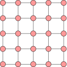
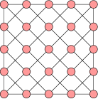
Figure 5.4. Examples of graphs belonging to two families which are not bi-iterative, because they have unbounded clique-width.

6. Graph polynomials and MSOL

We consider in this paper two related rich families of graph polynomials with useful decomposition properties. These graph polynomials are defined using a simple logical language on graphs.

6.1. Monadic Second Order Logic of graphs, MSOL

We define the logic MSOL of graphs inductively. We have three types of variables: $x_{i}:\,i\in\mathbb{N}$ which range over vertices, $U_{i}:\,i\in\mathbb{N}$ which range over sets of vertices and $B_{i}:\,i\in\mathbb{N}$ which range over sets of edges. We assume our graphs are ordered, i.e. that there exists an order relation $\leq$ on the vertices. Atomic formulas are of the form $x_{i}=x_{j}$, $(x_{i},x_{j})\in E$, $x_{i}\leq x_{j}$, $x_{i}\in U_{j}$ and $(x_{i},x_{j})\in B_{\ell}$. The logical formulas of MSOL are built inductively from the atomic formulas by using the connectives $\lor$ (or), $\land$ (and), $\neg$ (negation) and $\to$ (implication), and the quantifiers $\forall x_{i}$, $\exists x_{i}$, $\forall U_{i}$, $\exists U_{i}$, $\forall B_{i}$, $\exists B_{i}$ with their natural interpretation.

If no variable $B_{i}$ occurs in the formula, then the formula is said to be in MSOL_G, MSOL on graphs. Otherwise, the formula is said to be on hypergraphs. Sometimes additional modular quantifiers are allowed, giving rise to the extended logic CMSOL. The counting quantifiers are of the form $C_{q}x\,\varphi(x)$, whose semantics is that the number of elements from the universe satisfying $\varphi$ is zero modulo $q$. On structures containing an order relation, as is the case here, CMSOL and MSOL are equivalent, cf. [6].

Example 29.

1. We can express in MSOL that a set of edges $B_{1}$ is a matching:

   $$\varphi_{match}(B_{1})=\forall x_{1}\forall x_{2}\forall x_{3}\left((x_{1},x_{2})\in B_{1}\land(x_{2},x_{3})\in B_{1}\to x_{1}=x_{3}\right)$$

2. We can express in MSOL that a set of vertices $U_{1}$ is an independent set:

   $$\varphi_{ind}(U_{1})=\forall x_{1}\forall x_{2}\left((x_{1},x_{2})\in E\to\left(x_{1}\notin U_{1}\lor x_{2}\notin U_{1}\right)\right)$$

   where write e.g. $x_{1}\notin U_{1}$ as shorthand for $\neg\left(x_{1}\in U_{1}\right)$. Note $\varphi_{ind}(U_{1})$ is a MSOL_G formula.

3. A graphs is $3$-colorable iff it satisfies the following MSOL_G formula:

   $$\exists U_{1}\exists U_{2}\exists U_{3}\left(\varphi_{partition}(U_{1},U_{2},U_{3})\land\varphi_{ind}(U_{1})\land\varphi_{ind}(U_{2})\land\varphi_{ind}(U_{3})\right)$$

   where $\varphi_{partition}$ expresses that $U_{1},U_{2},U_{3}$ form a partition of the vertices:

   $$\varphi_{partition}(U_{1},U_{2},U_{3}) = \forall x_{1}\left(x_{1}\in U_{1}\lor x_{1}\in U_{2}\lor x_{1}\in U_{3}\right)\land$$

   $$\forall x_{1}\neg\left(x_{1}\in U_{1}\land x_{1}\in U_{2}\right)\land$$

   $$\forall x_{1}\neg\left(x_{1}\in U_{2}\land x_{1}\in U_{3}\right)\land$$

   $$\forall x_{1}\neg\left(x_{1}\in U_{1}\land x_{1}\in U_{3}\right)$$

4. We can express in MSOL that a vertex $x_{1}$ is the first element is its connected component in the graph spanned by $B_{1}$ with respect to the ordering of the vertices:

   $$\varphi_{fconn}(x_{1},B_{1})=\forall x_{2}\left(\varphi_{sc}(x_{1},x_{2})\to x_{1}\leq x_{2}\right)$$

   where $\varphi_{sc}(x_{1},x_{2})$ says that $x_{1}$ and $x_{2}$ belong to the same connected component in the graph spanned by $B_{1}$:

   $\begin{array}[]{rccl}\varphi_{sc}(x_{1},x_{2},B_{1})&=&\forall U_{1}&\Bigg{(}\bigg{(}x_{1}\in U_{1}\land x_{2}\notin U_{1}\bigg{)}\to\\ &&&\exists x_{3}\exists x_{4}\left(B_{1}(x_{3},x_{4})\land x_{3}\in U_{1}\land x_{2}\notin U_{1}\right)\Bigg{)}\end{array}$

   The formula $\varphi_{fconn}(x_{1},B_{1})$ will be useful when we discuss the definability of the Tutte polynomial.

6.2. MSOL-polynomials

MSOL-polynomials are a class of inductively defined graph polynomials given e.g. in [16]. It is convenient to refer to them in the following normal form:

$$p=\sum_{U_{1},\ldots,U_{\ell},B_{1},\ldots,B_{m}:\Phi(\bar{U},\bar{B})}\,\,X_{1}^{\left|U_{1}\right|}\cdots X_{\ell^{\prime}}^{\left|U_{\ell^{\prime}}\right|}X_{\ell^{\prime}+1}^{\left|B_{1}\right|}\cdots X_{\ell^{\prime}+m^{\prime}}^{\left|B_{m^{\prime}}\right|}$$

where $\Phi$ is an MSOL formula with the iteration variables indicated and $\ell^{\prime}\leq\ell$, $m^{\prime}\leq m$. $\bar{U},\bar{B}$ is short for $U_{1},\ldots,U_{\ell},B_{1},\ldots,B_{m}$. If $m=0$ and all the formulas are MSOL_G formulas, then we say $p$ is a MSOL_G-polynomial. It is often convenient to think of the indeterminates $X_{i}$ as multiplicative weights of vertices and edges.

While every MSOL_G-polynomial is a MSOL-polynomial, the converse is not true. The independence polynomial, the interlace polynomial [8], the domination polynomial and the vertex cover polynomial are MSOL_G-polynomials. The Tutte polynomial, the matching polynomial, the characteristic polynomial and the edge cover polynomial are MSOL_HG. We illustrate this for the independence polynomial and the Tutte polynomial.

6.3. The independence polynomial

The independence polynomial is the generating function of independent sets,

$$I(G)=\sum_{j=0}^{n}ind_{G}(j)X^{j}\,,$$

where $ind_{G}(j)$ is the number of independent sets of size $j$ and $n$ is the number of vertices in $G$. It is a MSOL_G-polynomial, given by

$$I(G)=\sum_{U_{1}:\Phi_{ind}(U_{1})}\,\,X^{|U_{1}|}$$

where $\Phi_{ind}=\varphi_{ind}$ from Example 29 says $U_{1}$ is an independent set.

6.4. The Tutte polynomial and the chromatic polynomial

The chromatic polynomial is defined in terms of counting proper colorings, but it can be written as a subset expansion which resembles an MSOL-polynomial as follows:

(6.1) $$\chi(G)=\sum_{A\subseteq E}(-1)^{|A|}X^{k(A)}$$

where $k(A)$ is the number of connected components in the spanning subgraph of $G$ with edge set $A$.

Therefore, $\chi(G)$ is an evaluation of the dichromatic polynomial given by

$$Z(G)=\sum_{A\subseteq E}Y^{|A|}X^{k(A)}$$

which is an MSOL-polynomial:

$$Z(G)=\sum_{U_{1},B_{1}:\Phi_{1}}\,\,Y^{|B_{1}|}X^{|U_{1}|}$$

with $\Phi_{1}$ says that $U_{1}$ is the set of vertices which are minimal in their connected component in the graph $(V,B_{1})$ with respect to the ordering on the vertices

$$\Phi_{1}=\forall x\left(x\in U_{1}\leftrightarrow\varphi_{fconn}(x_{1},B_{1})\right),$$

where $\varphi_{fconn}$ is from Example 29. The dichromatic polynomial is related to the Tutte polynomial via the following relation:

$$T(G,X,Y)=\frac{Z(G,(X-1)(Y-1),Y-1)}{(X-1)^{k(E)}(Y-1)^{|V|}}\,.$$

The Tutte polynomial can also be shown to be an MSOL-polynomial via its definition in terms of spanning trees.

6.5. A Feferman-Vaught-type theorem for MSOL-polynomials

The main technical tool from model theory that we use in this paper is a decomposition property for MSOL-polynomials, which resembles decomposition theorems for formulas of First Order Logic, FOL, and MSOL. For an extensive survey of the history and uses of Feferman-Vaught-type theorems, including to MSOL-polynomials, see [21].

In Theorem 30 we rephrase Theorem 6.4 of [21]. For simplicity, we do not introduce the general machinery that is used there, e.g. instead of the notion of MSOL-smoothness of binary operations we limit ourselves to our elementary operations (see Section 4 of [21] for more details). Some other small differences follow from the proof of Theorem 6.4.

Theorem 30 ([21], see also [11]).

Let $k$ be a natural number. Let $P$ be a finite set of MSOL-polynomials. Then there exists a finite set of MSOL-polynomials $P^{\prime}=\{p_{0},\ldots,p_{\alpha}\}$ such that $P\subseteq P^{\prime}$ and for every elementary operation $\sigma$ on $k$-graphs, the following holds. If either all members of $P$ are MSOL_G-polynomials, or $\sigma$ consists only of bounded basic operations, then there exists a matrix $M_{\sigma}$ such that for every graph $G$,

$$\left(p_{0}(\sigma(G),\bar{X}),\ldots,p_{\alpha}(\sigma(G),\bar{X})\right)^{tr}=M_{\sigma}\left(p_{0}(G,\bar{X}),\ldots,p_{\alpha}(G,\bar{X})\right)^{tr}$$

$M_{\sigma}$ is a matrix of size $\alpha\times\alpha$ of polynomials with indeterminates $\bar{X}$. Additionally, if all members of $P$ are MSOL_G-polynomials, then the same is true for $P^{\prime}$.

For bi-iterative families of graphs we prove the following result, which we will use in the proof of our main theorem.

Lemma 31.

Let $k$ be a natural number. Let $p$ be an MSOL-polynomial and let $G_{n}:\,n\in\mathbb{N}$ be a bi-iterative graph family. If $p$ is an MSOL_G-polynomial, or $G_{n}:\,n\in\mathbb{N}$ is bounded, then there exist a finite set of MSOL-polynomials $P^{\prime}=\{p_{0},\ldots,p_{\alpha}\}$ and a C-finite sequence $M_{n}:\,n\in\mathbb{N}$ such that $p\in P^{\prime}$ and

such that

$$\left(p_{0}(G_{n+1},\bar{X}),\ldots,p_{\alpha}(G_{n+1},\bar{X})\right)^{tr}=M_{n}\left(p_{0}(G_{n},\bar{X}),\ldots,p_{\alpha}(G_{n},\bar{X})\right)^{tr}$$

Additionally, if $p$ is an MSOL_G-polynomial, then the same is true for all members of $P^{\prime}$.

Proof.

Let $F$, $H$ and $L$ be elementary operations such that $G_{n+1}=H\left(F^{n}(L(G_{n}))\right)$. Let $P^{\prime}=\{p_{0},\ldots,p_{\alpha}\}$ be the set of MSOL-polynomials guaranteed in Theorem 30 for $P=\{p\}$. We have

$$\left(p_{0}(\sigma(G),\bar{X}),\ldots,p_{\alpha}(\sigma(G),\bar{X})\right)^{tr}=M_{\sigma}\left(p_{0}(G,\bar{X}),\ldots,p_{\alpha}(G,\bar{X})\right)^{tr}$$

for $\sigma\in\left\{L,F,H\right\}$. Therefore,

$$\left(p_{0}(G_{n+1},\bar{X}),\ldots,p_{\alpha}(G_{n+1},\bar{X})\right)^{tr}=M_{H}M_{F}^{n}M_{L}\left(p_{0}(G,\bar{X}),\ldots,p_{\alpha}(G,\bar{X})\right)^{tr}\,.$$

By Lemmas 11 and 12, $A_{n}=M_{H}M_{F}^{n}M_{L}$ is a C-finite sequence of matrices. ∎

7. Statement and proof of Theorem 2

We are now ready to state Theorem 2 exactly and prove it.

Theorem 32.

Let $k$ be a natural number. Let $p$ be an MSOL-polynomial and let $G_{n}:\,n\in\mathbb{N}$ be a bi-iterative graph family. If $p$ is an MSOL_G-polynomial, or $G_{n}:\,n\in\mathbb{N}$ is bounded, then the sequence $p(G_{n}):\,n\in\mathbb{N}$ is C${\,}^{2}$-finite.

To transfer Theorem 32 to C-finite sequences over a polynomial ring, we will use the following lemma:

Lemma 33.

Let $\mathbb{F}$ be a countable subfield of $\mathbb{C}$. For every $\xi\in\mathbb{N}$, there exists a set $D_{\xi}=\{d_{1},\ldots,d_{\xi}\}\subseteq\mathbb{R}$ such that the partial function $sub_{\xi}:\mathbb{F}[x_{1},\ldots,x_{\xi}]\to\mathbb{C}$ given by

$$sub_{\xi}(p)=p(d_{1},\ldots,d_{\xi})$$

is injective.

Proof.

We prove the claim by induction on $\xi$. For the case $\xi=0$ we have $D_{\xi}=\emptyset$ and $sub_{\xi}(p)=p$, which is injective.

Now assume there exists $D_{\xi-1}$ such that $sub_{\xi-1}$ is injective. Let $B_{\xi-1}$ be the set of real numbers which are roots of non-zero polynomials in the polynomial ring $\mathbb{F}[d_{1},\ldots,d_{\xi-1}][x_{\xi}]$ of polynomials in the indeterminate $x_{\xi}$ whose coefficients are polynomials in $d_{1},\ldots,d_{\xi-1}$ with rational coefficients. The cardinality of $B_{\xi-1}$ is $\aleph_{0}$, implying that that there exists $d_{\xi}\in\mathbb{R}\backslash B_{\xi-1}$. Let $D_{\xi}=D_{\xi-1}\cup\{d_{\xi}\}$. Assume for contradiction that there exist distinct $p,q\in\mathbb{Q}[x_{1},\ldots,x_{\xi}]$ such that $sub_{\xi}(p)=sub_{\xi}(q)$. Let $r(x_{1},\ldots,x_{\xi})=p(x_{1},\ldots,x_{\xi})-q(x_{1},\ldots,x_{\xi})$. Let

$$r(x_{1},\ldots,x_{\xi})=\sum_{i_{1},\ldots,i_{\xi}\leq t}\rho_{i_{1},\ldots,i_{\xi}}x_{1}^{i_{1}}\cdots x_{\xi}^{i_{\xi}}\,.$$

Since $p$ and $q$ are distinct, $r$ is not the zero polynomial and there exists $i_{\xi}^{\prime}$ such that

$$r_{i_{\xi}^{\prime}}(x_{1},\ldots,x_{\xi-1})=\sum_{i_{1},\ldots,i_{\xi-1}\leq t}\rho_{i_{1},\ldots,i_{\xi-1},i_{\xi}^{\prime}}x_{1}^{i_{1}}\cdots x_{\xi-1}^{i_{\xi-1}}$$

is not identically non-zero.

By the assumption that $sub_{\xi}(p)=sub_{\xi}(q)$ we have that $r(d_{1},\ldots,d_{\xi})=0$.

• If $x_{\xi}$ has non-zero degree in $r(d_{1},\ldots,d_{\xi-1},x_{\xi})$, then $d_{\xi}$ is indeed a root of a non-zero polynomial $r(d_{1},\ldots,d_{\xi-1},x_{\xi})\in\mathbb{Q}[d_{1},\ldots,d_{\xi-1}][x_{\xi}]$.

• Otherwise, $r(d_{1},\ldots,d_{\xi-1},x_{\xi})$ is a polynomial of degree zero in $x_{\xi}$. In order for $r(d_{1},\ldots,d_{\xi})=0$ to hold, $r(d_{1},\ldots,d_{\xi-1},x_{\xi})$ must be identically zero. In particular, the coefficient of $x_{\xi}^{i_{\xi}^{\prime}}$ in $r(d_{1},\ldots,d_{\xi-1},x_{\xi})$ is zero, but this coefficient is $r_{i_{\xi}^{\prime}}(d_{1},\ldots,d_{\xi-1})$. This implies that there exist two distinct polynomials, e.g. $r_{i_{\xi}^{\prime}}(\bar{x})$ and $2r_{i_{\xi}^{\prime}}(\bar{x})$, which agree on $d_{1},\ldots,d_{\xi-1}$ in contradiction to the assumption that $sub_{\xi-1}$ is injective.

∎

Lemma 34.

Let $\mathbb{F}$ be a subfield of $\mathbb{C}$ and let $r\in\mathbb{N}^{+}$ and let $r\in\mathbb{N}^{+}$. For every $n\in\mathbb{N}^{+}$, let $\overline{v_{n}}$ be a column vector of size $r\times 1$ of polynomials in $\mathbb{F}[x_{1},\ldots,x_{k}]$. Let $M_{n}$ be a C-finite sequence of matrices of size $r\times r$ over $\mathbb{F}[x_{1},\ldots,x_{k}]$ such that, for every $n$,

(7.1) $$\overline{v_{n+1}}=M_{n}\overline{v_{n}}\,.$$

For each $j=1,\dots,r$, $\overline{v_{n}}[j]$ is C${\,}^{2}$-finite. Moreover, all of the $\overline{v_{n}}[j]$ satisfy the same recurrence relation (possibly with different initial conditions).

Proof.

First note that due to the C-finiteness of $M_{n}$ and Eq. (7.1), we may assume w.l.o.g. that the the matrices $M_{n}$ and vectors $\overline{v_{n}}$ are all given over a finite extension field $\mathbb{F}$ of $\mathbb{C}$. In particular, we need that $\mathbb{F}$ is countable.

Let $D_{k}=\{d_{1},\ldots,d_{k}\}$ be the set guaranteed in Lemma 33. For every $n$, let $\overline{u_{n}}$ and $L_{n}$ be the real vector respectively real matrix obtained from $\overline{v_{n}}$ respectively $M_{n}$ by substituting $x_{1},\ldots,x_{k}$ with $d_{1},\ldots,d_{k}$. $L_{n}$ is a C-finite sequence of matrices over $\mathbb{F}(d_{1},\ldots,d_{k})$ the extension field of $\mathbb{F}$ with $D_{k}$. We have for every $n$,

$$\overline{u_{n+1}}=L_{n}\overline{u_{n}}\,.$$

By Lemma 14, there exists $n_{0}$ and C-finite sequences over $\mathbb{F}(d_{1},\ldots,d_{k})$,$c_{n}^{\{0\}},\ldots,c_{n}^{\{r^{2}\}}$, such that for every $n>n_{0}$,

$$c_{n}^{\{0\}}\overline{u_{n}}+\cdots+c_{n}^{\{r^{2}-1\}}\overline{u_{n+r^{2}-1}}=c_{n}^{\{r^{2}\}}\overline{u_{n+r^{2}}}$$

and $q_{n}^{\{r^{2}\}}$ is non-zero. Using Lemma 33, there exist unique polynomials

$$q_{n}^{\{0\}}(x_{1},\ldots,x_{\xi}),\ldots,q_{n}^{\{r^{2}\}}(x_{1},\ldots,x_{\xi})$$

such that for every $n$,

$$q_{n}^{\{0\}}(d_{1},\ldots,d_{\xi})=c_{n}^{\{0\}}(d_{1},\ldots,d_{\xi})\,.$$

Let $t(x_{1},\ldots,x_{\xi})$ be the polynomial given by

$$t(x_{1},\ldots,x_{\xi})=q_{n}^{\{0\}}\overline{v_{n}}+\cdots+q_{n}^{\{r^{2}-1\}}\overline{v_{n+r^{2}-1}}-q_{n}^{\{r^{2}\}}\overline{v_{n+r^{2}}}\,.$$

substituting $d_{1},\ldots,d_{\xi}$ on both sides of the latter equation, we get $sub_{\xi}(t)=0$, but this implies that $t(x_{1},\ldots,x_{\xi})$ is identically zero, since $sub_{\xi}(0)=0$ and $sub_{\xi}$ is injective.

∎

Proof of Theorem 32.

Let $P^{\prime}=\{p_{0},\ldots,p_{\alpha}\}$ and $M_{n}:\,n\in\mathbb{N}$ be as guaranteed by Lemma 31. We have

$$\left(p_{0}(G_{n+1},\bar{X}),\ldots,p_{\alpha}(G_{n+1},\bar{X})\right)^{tr}=M_{n}\left(p_{0}(G_{n},\bar{X}),\ldots,p_{\alpha}(G_{n},\bar{X})\right)^{tr}\,.$$

By Lemma 34, $p(G_{n}):\,n\in\mathbb{N}$ is C²-finite. ∎

8. Examples of relatively iterative sequences

Here we give explicit applications of Theorem 2. The applications follow the basic ideas underlying the proof, but can be significantly simplified given specific choices of a graph polynomial and a bi-iterative family.

8.1. The independence polynomial on $G_{n}^{2}$

Let $G_{n}^{2}$ be as described in Example 16. We denote by $v_{0},\ldots,v_{n}$ the vertices of the underlying path of $G_{n}^{2}$. Let $I_{A}(G_{n}^{2},x)$ ($I_{B}(G_{n}^{2},x)$) be the generating functions counting independent sets $U_{1}$ in $G_{n}^{2}$ such that $v_{n}$ belongs (resp. does not belong) to $U_{1}$. Then,

(8.1) $$I(G_{n}^{2},x)=I_{A}(G_{n}^{2},x)+I_{B}(G_{n}^{2},x)\,.$$

Now we give a matrix equation for computing $I_{A}(G_{n+1}^{2},x)$,$I_{B}(G_{n+1}^{2},x)$ and $I(G_{n+1}^{2},x)$ from $I_{A}(G_{n}^{2},x)$,$I_{B}(G_{n}^{2},x)$ and $I(G_{n}^{2},x)$: for all $m$,

(8.6) $$\left(\begin{array}[]{c}I_{A}(G_{m+1}^{2},x)\\ I_{B}(G_{m+1}^{2},x)\end{array}\right) = M\left(\begin{array}[]{c}I_{A}(G_{m}^{2},x)\\ I_{B}(G_{m}^{2},x)\end{array}\right)$$

where

$$M=\left(\begin{array}[]{cc}0&x\\ 1+nx&1+nx\end{array}\right)\,.$$

The first row reflects the facts that if $v_{n+1}$ belongs to the sets $U_{1}$ counted by $I_{A}(G_{n+1}^{2},x)$, $v_{n+1}$ and $v_{n}$ may not belong to the same $U_{1}$, and $v_{n+1}$ contributes a multiplicative factor of $x$. The second row reflects that $v_{n+1}$ does not belong to the sets $U_{1}$ counted in $I_{B}(G_{n+1}^{2},x)$, so independent of whether $v_{n}$ is in $U_{1}$, there are two options: either exactly one of the clique vertices adjacent to $v_{n+1}$ belong to $U_{1}$ and contributes a factor of $x$, or no vertex of that clique belongs to $U_{1}$, contributing a factor of $1$.

Eq. (8.6) holds both for $n$ and $n+1$, leading to the recurrence relation

$$I(G_{n+1}^{2},x) = (1+nx)I(G_{n}^{2},x)+x(1+(n-1)x)I(G_{n-1}^{2},x)$$

$$I(G_{0}^{2},x) = 1+x$$

$$I(G_{1}^{2},x) = 1+3x+x^{2}$$

using Eq. (8.1). This is a C²-finite recurrence, which is also a P-recurrence.

The number of independent sets of $G_{n+1}^{2}$ is $I(G_{n+1}^{2},1)$. Interestingly, the sequence $I(G_{n+1}^{2},1):n\in\mathbb{N}$ is in fact equal to the seemingly unrelated sequence (A052169) of [1]. This implies $I(G_{n+1}^{2},1)$ has an alternative combinatorial interpretation as the number of non-derangements of $1,\ldots,n+3$ divided by $n+2$. See [25] for a treatment of the related (A002467).

8.2. The dichromatic polynomial on $G_{n}^{4}$

Let $Z_{t}(P_{n+2})$ denote the dichromatic polynomial of $P_{n+2}$ such that the end-points of $P_{n+2}$ belong to the same connected component iff $t=1$, for $t=0,1$. $Z_{t}(G_{n}^{4})$ is defined similarly with respect to the most recently added path.

We have

$$Z_{0}(G_{n}^{4}) = \left(\frac{v}{q}+1\right)^{2}Z_{0}(P_{n+2})\cdot Z_{0}(G_{n-1}^{4})$$

$$+\left(2\frac{v}{q}+1\right)Z_{0}(P_{n+2})Z_{1}(G_{n-1}^{4})$$

$$Z_{1}(G_{n}^{4}) = \frac{v^{2}}{q^{2}}Z_{0}(P_{n+2})Z_{1}(G_{n-1}^{4})$$

$$+\left(\frac{v^{2}}{q}+2\frac{v}{q}+1\right)Z_{1}(P_{n+2})Z_{1}(G_{n-1}^{4})$$

$$+\left(\frac{v}{q}+1\right)^{2}Z_{1}(P_{n+2})Z_{0}(G_{n-1}^{4})$$

by dividing into cases by considering the end-points $u,v$ of $P_{n+2}$ and the end-points $u^{\prime},v^{\prime}$ of the $P_{n+1}$ in $G_{n-1}^{4}$ and the edges $\{u,v\}$ and $\{u^{\prime},v^{\prime}\}$ with respect to the iteration variable of $Z_{t}(G_{n}^{4})$. For example, the coefficient of $Z_{1}(P_{n})Z_{1}(G_{n-1}^{4})$ corresponds exactly to the case that $u,v$ are in the same connected components in the graph spanned by $A$ ($A$ is the iteration variable in the definition of $Z$ in Eq. (6.1)). If at least one of the edges $\{u,v\}$ and $\{u^{\prime},v^{\prime}\}$ belongs to $A$, then $G_{n-1}^{4}$ and $G_{n}^{4}$ have the same number of connected components, but in $Z_{1}(P_{n+2})Z_{1}(G_{n-1}^{4})$ we have that $Z_{1}(P_{n+2})$ contributes an additional factor of $q$ which should be cancelled, so the weight in the case is $\frac{v^{2}+2v}{q}$. If none of the two edges belongs to $A$, then $u,v$ are in a different connected component from $u^{\prime},v^{\prime}$, so no correction is needed and the weight is $1$.

Using that $Z(G_{n}^{4})=Z_{0}(G_{n}^{4})+Z_{1}(G_{n}^{4})$, we get:

(8.7) $$Z_{0}(G_{n}^{4}) = \frac{v^{2}}{q^{2}}Z_{0}(P_{n+2})\cdot Z_{0}(G_{n-1}^{4})$$

$$+\left(2\frac{v}{q}+1\right)Z_{0}(P_{n+2})Z(G_{n-1}^{4})$$

(8.8) $$Z(G_{n}^{4}) = \left(\left(\frac{v}{q}+1\right)^{2}Z(P_{n+2})+\frac{v^{2}}{q}\left(1-\frac{1}{q}\right)Z_{1}(P_{n+2})\right)Z(G_{n-1}^{4})$$

$$-\frac{v^{2}}{q}\left(1-\frac{1}{q}\right)Z_{1}(P_{n+2})Z_{0}(G_{n-1}^{4})$$

Let $m\in\mathbb{N}$. Eqs. (8.7) and (8.8) hold for every $n$, in particular for $m$ and $m+1$, and from these equations we can extract a recurrence relation for $Z(G_{m+1}^{4})$ using $Z(G_{m}^{4})$ and $Z(G_{m-1}^{4})$ by canceling out $Z_{0}(G_{m}^{4})$ and $Z_{0}(G_{m-1}^{4})$:

$$Z(G_{m+1}^{4}) = Z(G_{m}^{4})\left(\left(\frac{v}{q}+1\right)^{2}Z(P_{m+3})+\frac{v^{2}}{q}\left(1-\frac{1}{q}\right)Z_{1}(P_{m+3})\right)$$

$$-Z(G_{n-1}^{4})\Bigg{[}\frac{v^{2}}{q}\left(1-\frac{1}{q}\right)Z_{1}(P_{m+3})\cdot\Bigg{(}Z_{0}(P_{m+2})\frac{v^{2}}{q^{2}}+$$

$$\frac{\left(\frac{v}{q}+1\right)^{2}Z_{0}(P_{m+2})Z(P_{m+2})}{\left(q-1\right)Z_{1}(P_{m+2})}+\left(2\frac{v}{q}+1\right)Z_{0}(P_{m+2})\Bigg{)}\Bigg{]}$$

Using this recurrence relation, it is easy to compute the dichromatic and Tutte polynomials. E.g., $Z(G_{m}^{4},3,-1)$, the number of $3$-proper colorings of $G_{m}^{4}$, and $|Z(G_{m}^{4},-1,-1)|$, the number of acyclic orientations of $G_{m}^{4}$, are given, for $m=0,\ldots,6$, by

$$Z(G_{m}^{4},3,-1):$$ 6 30 318 6762 288354 24601830 4198550862

$$|Z(G_{m}^{4},-1,-1)|:$$ 6 90 2826 179874 22988394 5882561010 3011536790874

9. Conclusion and further research

We introduced a natural type of recurrence relations, C²-recurrences, and proved a general theorem stating that a wide class of graph polynomials have recurrences of this type on some families of graphs. We gave explicit applications to the Tutte polynomial and the independence set polynomial. We further showed that quadratic sub-sequence of C-finite sequences are C²-finite.

A natural generalization of the notion of C²-recurrences could be to allow even sparser sub-sequences. We say a sequence $a_{n}$ is C¹-finite if it is C-finite. We say a sequence is C${}^{\,r}$-finite if it has a linear recurrence relation of the form

$$c_{n}^{(s)}a_{n+s}=c_{n}^{(s-1)}a_{n+s-1}+\cdots+c_{n}^{(0)}a_{n}$$

where $c_{n}^{(0)},\ldots,c_{n}^{(s)}$ are C^r-1-finite. This definition coincides with the definition of C²-finite.

Problem 35.

Can we find families of graphs for which the Tutte polynomial and other MSOL-polynomials have C^r-recurrences?

References

- [1] The On-Line Encyclopedia of Integer Sequences, 2013. published electronically at http://oeis.org.
- [2] J. P. Bell, S. N. Burris, and K. Yeats. On the set of zero coefficients of a function satisfying a linear differential equation. Mathematical Proceedings of the Cambridge Philosophical Society, 153:235–247, 9 2012.
- [3] A. Ben-Israel and T.N.E. Greville. Generalized Inverses: Theory and Applications. CMS Books in Mathematics. Springer, 2003.
- [4] N.L Biggs, R.M Damerell, and D.A Sands. Recursive families of graphs. Journal of Combinatorial Theory, Series B, 12(2):123 – 131, 1972.
- [5] Colleen Bouey, Christina Graves, Aaron Ostrander, and Gregory Palma. Non-recursively constructible recursive families of graphs. Electr. J. Comb., 19(2):P9, 2012.
- [6] B. Courcelle and J. Engelfriet. Graph Structure and Monadic Second-Order Logic: A Language-Theoretic Approach. Encyclopedia of Mathematics and its Applications. Cambridge University Press, 2012.
- [7] B. Courcelle, J. A. Makowsky, and U. Rotics. Linear time solvable optimization problems on graphs of bounded clique-width. Theory of Computing Systems, 33(2):125–150, 2000.
- [8] Bruno Courcelle. A multivariate interlace polynomial and its computation for graphs of bounded clique-width. Electr. J. Comb., 15(1), 2008.
- [9] Bruno Courcelle and Stephan Olariu. Upper bounds to the clique width of graphs. Discrete Applied Mathematics, 101(1-3):77–114, 2000.
- [10] Jacques Désarménien and Michelle L. Wachs. Descent classes of permutations with a given number of fixed points. J. Comb. Theory Ser. A, 64(2):311–328, November 1993.
- [11] E. Fischer and J.A. Makowsky. Linear recurrence relations for graph polynomials. In Pillars of Computer Science, volume 4800 of Lecture Notes in Computer Science, pages 266–279. Springer, 2008.
- [12] Stavros Garoufalidis and Thang T Q Lê. The colored Jones function is q-holonomic. Geometry & Topology, 2005.
- [13] R. Gelca. Non-commutative trigonometry and the a-polynomial of the trefoil knot. Mathematical Proceedings of the Cambridge Philosophical Society, 133:311–323, 9 2002.
- [14] R. Gelca and J. Sain. The noncommutative a-ideal of a (2, 2p + 1)-torus knot determines its Jones polynomial. Journal of Knot Theory and Its Ramifications, 12(02):187–201, 2003.
- [15] Ira M Gessel and Christophe Reutenauer. Counting permutations with given cycle structure and descent set. Journal of Combinatorial Theory, Series A, 64(2):189 – 215, 1993.
- [16] B. Godlin, T. Kotek, and J.A. Makowsky. Evaluations of graph polynomials. In Workshop on Graph Theoretic Concepts in Computer Science (WG), pages 183–194, 2008.
- [17] Sang il Oum and Paul Seymour. Approximating clique-width and branch-width. Journal of Combinatorial Theory, Series B, 96(4):514 – 528, 2006.
- [18] T. Kotek and J.A. Makowsky. Connection matrices and the definability of graph parameters. In Computer Science Logic (CSL), 2012.
- [19] V. E. Levit and E. Mandrescu. The independence polynomial of a graph–a survey. In Proceedings of the 1st International Conference on Algebraic Informatics, pages 223–254, 2005.
- [20] L. Lovász. Large Networks and Graph Limits. American Mathematical Society colloquium publications. American Mathematical Society, 2012.
- [21] J.A. Makowsky. Algorithmic uses of the Feferman-Vaught theorem. Annals of Pure and Applied Logic, 126(1-3):159–213, 2004.
- [22] J.A. Makowsky. Coloured Tutte polynomials and Kauffman brackets for graphs of bounded tree width. Discrete Applied Mathematics, 145(2):276–290, 2005.
- [23] M. Noy and A. Ribó. Recursively constructible families of graphs. Advances in Applied Mathematics, 32:350–363, 2004.
- [24] M. Petkovšek, H.S. Wilf, and D. Zeilberger. . A. K. Peters, Wellesley, MA, 1996.
- [25] Alexsandar Petojevic. The function and some well-known sequences. Journal of Integer Sequences, 5, 2002. Article 02.1.7.
- [26] R.P. Stanley. Enumerative combinatorics, volume 1. Cambridge University Press, 1986.
- [27] R.P. Stanley. Enumerative combinatorics, volume 2. Cambridge University Press, 1999.
- [28] Michelle L. Wachs. On q-derangement numbers. Proceedings of the American Mathematical Society, 106(1):273–278, 1989.
- [29] Yi Wang and Bao-Xuan Zhu. On the unimodality of independence polynomials of some graphs. European Journal of Combinatorics, 32(1):10 – 20, 2011.